Purely hydrodynamic origin for swarming of swimming particles

Abstract

Three-dimensional simulations with fully resolved hydrodynamics are performed to study the collective motion of model swimmers in confinement. We show that certain swimming mechanisms can lead to traveling wave-like collective motion even without any direct alignment mechanism. It is also shown that by varying the swimming mechanism, this collective motion can be suppressed, contrary to the perception that hydrodynamic effects are completely screened at high volume fraction. From an analysis of bulk systems, it is shown that this traveling wave-like motion, which can be characterized as a pseudo-acoustic mode, is mainly due to the intrinsic swimming property of the particles.

Active matter systems such as groups of microorganisms, birds or fish often form swarms or flocks, and typically show complex collective behavior Sokolov et al. (2007); Nash et al. (2010); Mishra (2014). Of special interest for scientific study are active microscopic systems, e.g. microorganisms or Janus particles, because they are particularly well suited for experiments. Understanding the collective dynamic behavior of these systems can be useful for both science and industrial applications, for example, to explain the formation of biofilms Nadell et al. (2009) or to design targeted drug delivery systems Laage (2006). Such systems typically exist under some type of confinement, which has been shown to exert a strong influence on the collective behavior Angelani et al. (2009); Di Leonardo et al. (2010); Woodhouse and Goldstein (2012); Kaiser et al. (2012, 2014). So far, most analysis of such systems have either neglected hydrodynamic interactions or only considered them in a far field approximation Aditi Simha and Ramaswamy (2002); Angelani et al. (2009); Kaiser et al. (2012); Ezhilan et al. (2013), even though it is known that the hydrodynamic interactions can dramatically affect the physical properties of the systems Rafaï et al. (2010). Theoretically, it’s impossible to take into account the full hydrodynamic interactions in many body systems, and numerically it’s very computationally expensive. While several studies have succeeded in including hydrodynamic interactions Evans et al. (2011); Alarcon and Pagonabarraga (2013); Li and Ardekani (2014), none have focused on the collective dynamic behavior of 3D active systems under confinement. The recent work by Zöttl and StarkZöttl and Stark (2014) is related to ours, but deals with pseudo-2D systems under strong confinement (small separation of walls), high volume fraction and strong swimming strength, which are quite different conditions from those of the present work. Not surprisingly, we are able to observe quite different dynamic behavior.

We have conducted direct numerical calculations for 3D systems of spherical swimmers in a host viscous fluid with fully resolved hydrodynamics. Under the confinement of two flat parallel walls, we find collective motion of swimmers with traveling wave characteristics, which propagates back and forth between the walls. Although similar traveling wave-like motion has already been observed in systems with explicit alignment interactions between the particles Chaté et al. (2008); Ohta and Yamanaka (2014), here we show that hydrodynamic interactions alone are enough to exhibit this behavior. We also confirmed that this traveling wave-like behavior is not due to the presence of the walls, but is just a manifestation of the bulk behavior. Crucial to observe this behavior are the strength and type (pushers vs. pullers) of swimming, not the degree of global alignment.

As the numerical model of microswimmers, the Squirmer Model was employed. In this model, a self-propelled particle is modeled as a spherical object with a modified stick boundary condition at its surface Lighthill (1952); Blake (1971):

$$\boldsymbol{u}^{s}\left(\hat{\boldsymbol{r}}\right)=\sum_{i=1}^{\infty}\frac{2}{n(n+1)}B_{n}P_{n}^{\prime}(\cos{\theta})\sin{\theta}\hat{\boldsymbol{\theta}},$$ (1)

where $\hat{\boldsymbol{r}}$ is a unit vector directed from the center of a squirmer to a point on its surface, $\theta=\cos^{-1}{(\hat{\boldsymbol{r}}\cdot\hat{\boldsymbol{e}})}$ the polar angle between $\hat{\boldsymbol{r}}$ and the swimming direction $\hat{\boldsymbol{e}}$, $\hat{\boldsymbol{\theta}}$ the unit polar angle vector. $P_{n}^{\prime}$ is the derivative of the Legendre polynomial of $n$-th order, and $B_{n}$ is the magnitude of each mode. Here, the radial deformation has been ignored, so this surface velocity has only the tangential component, and is responsible for the self-propulsion of the swimmers.

In this work, only the first two modes in Eq.(1) were retained:

$$\boldsymbol{u}^{s}(\theta)=B_{1}\left(\sin{\theta}+\frac{\alpha}{2}\sin{2\theta}\right)\hat{\boldsymbol{\theta}}.$$ (2)

The coefficient of the first mode, $B_{1}$, determines the swimming velocity of an isolated squirmer, as $U_{0}=2/3B_{1}$. The coefficient of the second mode, $B_{2}$, determines the strength of stirring, or the stresslet Ishikawa and Pedley (2007). Using only the first two modes, the type of swimming can be modified by changing the sign of the second coefficient, $\alpha$ in Eq.(2). Negative values of $\alpha$ describe pushers, which generate an extensile flow field in the propeling direction, and positive values describe pullers, which generate a contractile flow (Fig. 1). Because these two swimming mechanisms result in distinct flow fields, different swimmers can exhibit vastly different collective motion, as we will show in this paper.

Figure 1: Schematic representation of pushers and pullers within the squirmer model. The swimming direction, and the fluid and surface flows generated by squirmers are shown.

In this study, the squirmer model is incorporated into the Smoothed Profile Method (SPM) Nakayama and Yamamoto (2005); Kim et al. (2006); Nakayama et al. (2008), which is an efficient calculation scheme for solid/fluid two phase dynamics problems with full hydrodynamics. In this method, the sharp boundary between the solid and fluid domains is not considered explicitly. Instead, a diffuse interface of finite width $\zeta$ is introduced, and the solid domain is represented via an order parameter $\phi$, which takes a value of 1 in the solid domain, and 0 in the fluid domain. Using this continuous order parameter, all the physical quantities can be expressed as field variables on Cartesian grids, and the calculation cost can be reduced drastically. As the governing equations for the total fluid, we employ a modified incompressible Navier-Stokes equation:

$$\rho_{\text{f}}\left(\partial_{t}+\boldsymbol{u}\cdot\nabla\right)\boldsymbol{u} =\nabla\cdot\boldsymbol{\sigma}+\rho_{\text{f}}\left(\phi\boldsymbol{f}_{\text{p}}+\boldsymbol{f}_{\text{sq}}\right),$$

$$\boldsymbol{\nabla}\cdot\boldsymbol{u} =0,$$ (3)

$$\boldsymbol{u} =(1-\phi)\boldsymbol{u}_{\text{f}}+\phi\boldsymbol{u}_{\text{p}},$$

$$\phi\boldsymbol{u}_{\text{p}} =\sum_{i}\phi_{i}[\boldsymbol{V}_{i}+\boldsymbol{\Omega}_{i}\times\boldsymbol{R}_{i}],$$

where $\boldsymbol{u}$ is the total velocity field, $(1-\phi)\boldsymbol{u}_{\text{f}}$ and $\phi\boldsymbol{u}_{\text{p}}$ the velocity field of fluid and particles, respectively. The position, velocity and angular velocity of particle $i$ are expressed as $\boldsymbol{R}_{i}$, $\boldsymbol{V}_{i}$ and $\boldsymbol{\Omega}_{i}$. The stress tensor and the mass density of the host fluid are $\boldsymbol{\sigma}$, $\rho_{\text{f}}$. The body force generated from the rigidity condition of particles is calculated as $\phi\boldsymbol{f}_{\text{p}}$, and $\boldsymbol{f}_{\text{sq}}$ stands for the force field resulting from the squirming motion Molina et al. (2013). The time evolution of the particles follows from the Newton-Euler equations:

$$\dot{\boldsymbol{R}}_{i} =\boldsymbol{V}_{i}, \dot{\boldsymbol{Q}}_{i} =\text{skew}(\boldsymbol{\Omega}_{i})\cdot\boldsymbol{Q}_{i},$$ (4)

$$M_{\text{p}}\dot{\boldsymbol{V}}_{i} =\boldsymbol{F}_{i}^{\text{H}}+\boldsymbol{F}_{i}^{\text{C}}, \boldsymbol{I}_{\text{p}}\cdot\dot{\boldsymbol{\Omega}}_{i} =\boldsymbol{N}_{i}^{\text{H}},$$

where $\boldsymbol{Q}_{i}$ denotes the rotation matrix, $M_{\text{p}}$ the mass, $\text{skew}(\boldsymbol{\Omega}_{i})$ the skew symmetric matrix of $\boldsymbol{\Omega}_{i}$, and $\boldsymbol{F}_{i}^{\text{H}}$ and $\boldsymbol{N}_{i}^{\text{H}}$ are the hydrodynamic force and torque acting on particle $i$. The force due to direct interactions between particles, $\boldsymbol{F}_{i}^{\text{C}}$, is taken to be a truncated Lennard-Jones potential, in order to ensure that the excluded volume constraint is satisfied. See refs Nakayama and Yamamoto (2005); Kim et al. (2006); Nakayama et al. (2008); Molina et al. (2013) for more detailed information of this method.

Using this computational model, we conducted simulations of squirmer dispersion systems in a three dimensional domain. Throughout this paper, the diameter $a$ and the boundary thickness $\zeta$ of the squirmers are $4\Delta$, $2\Delta$, where $\Delta$ is the grid spacing and the unit length, and the parameter $B_{1}$ in Eq. (2) is 0.375, respectively. The shear viscosity $\eta$ and the fluid mass density $\rho_{\text{f}}$ are set to one, and the unit time is then expressed as $\rho\Delta^{2}/\mu$. The particle Reynolds number of an isolated squirmer $Re^{0}=\rho_{\text{f}}U_{0}a/\eta$ is set equal to one. The Reynolds number in the dispersion will be different from $Re^{0}$ due to a decrease in the propelling velocity with increasing volume fraction. We have ignored any effects due to thermal fluctuations. No external force is exerted, and the systems are buoyancy free.

We first calculated the dynamics of $N=2607$ swimmers in a $64\Delta\times 160\Delta\times 64\Delta$ rectangular system (volume fraction of 13%). The computational domain is periodic in the $x$ and $z$ direction, but confined between two flat parallel walls along the $y$ direction; at $y=1\Delta$ and $159\Delta$. These walls are made of $2048$ spherical particles which are pinned and unable to move or rotate from the initial positions and orientations. The wall particles are regularly spaced and are defined to have the same diameter as the squirmers. The initial configuration of swimmers was randomly determined with respect to both position and orientation. We conducted simulations for various $\alpha$ values in order to investigate the effect of $\alpha$ on the dynamics. We have calculated the time evolution of the local density $\rho$, polar order $Q_{\text{l}}$ and velocity $v_{\text{l}}$, as a function of distance from the walls. Here, $Q_{\text{l}}=\langle\hat{e}_{y}\rangle_{\text{plane}}$ and $\bar{v}_{\text{l}}=\langle{V}_{y}/U_{0}\rangle_{\text{plane}}$, where $\hat{e}_{y}$ and $V_{y}$ are the components of $\hat{\boldsymbol{e}}$ and $\boldsymbol{V}$ perpendicular to the walls, and $\langle\cdot\rangle_{\text{plane}}$ denotes an ensemble average over all particles in parallel slabs of width $2\Delta$. Fig. 2 shows the results of the systems with $\alpha=\pm 0.5$ (see supplementary materials S1 and S2). For pullers ($\alpha=0.5$), the time evolution of the density, polar order and velocity are shown, while for pushers ($\alpha=-0.5$), only density is shown. Only the pullers show large density fluctuations, which we note are due to hydrodynamic interactions alone, as no direct alignment interaction has been included; pushers show no such behavior. First, the pullers build up two distinct traveling waves which bounce back and forth between the walls. Gradually, as one wave begins to dominate, they merge into a single propagating wave. We also considered different wall separations, and found that such propagating wave-like motion can only be observed if the wall separation is larger than the characteristic size of this propagating flock. In our simulations, the threshold is $W/a\simeq 40$, where $W$ is the wall separation. In fig. 3, the traveling wave velocity is plotted for several different wall separations (the bulk sound velocity which will be explained later is also shown). They are quantitatively the same and there is no clear separation dependence. From these measurements, this traveling wave-like motion can be understood as an intrinsic property of the self-propelled systems, which is independent of the wall effects.

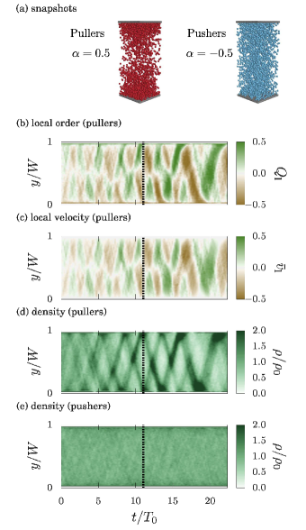
Figure 2: Simulation results for pullers and pushers ($\alpha=\pm 0.5$) at volume fraction of 13% and wall separation $W/a=40$. (a) Simulation snapshots at $T=11T_{0}$, (b) local order of pullers defined as $Q_{\text{l}}=\langle\hat{e}_{y}\rangle_{\text{plane}}$, (c) local velocity of pullers in y direction (perpendicular to the walls) defined as $\bar{v}_{\text{l}}=\langle{V}_{y}/U_{0}\rangle_{\text{plane}}$ (d,e) plane averaged density for pushers and pullers at each height $y/W$. The density is normalized by the global average value, $\rho_{0}$, and time and velocity are normalized by $T_{0}=W/U_{0}$ and $U_{0}$, where $W$ represents the separation of parallel flat walls. The snapshots are of around $t=11T_{0}$, which is marked by dashed line.

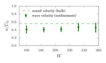
Figure 3: The traveling wave velocity of confined systems as a function of wall separation $W$. The sound velocity of the bulk system is also shown. Here, only puller results are shown, as pushers don’t show wave-like behavior. All the values are normalized by $U_{0}$.

To confirm this conjecture, further simulations were conducted in cubic systems with no confinement, under full periodic boundary conditions in all directions. The linear dimension of the computational domain is $L=64\Delta$ and the number of swimmers is $1043$ ( volume fraction of 13 %, the same value as the previous simulations in the systems with walls). In order to study the density correlations, we calculated the dynamic structure factor $S\left(\boldsymbol{k},\omega\right)$, which is just the Fourier transform (in both space and time) of the density-density correlation functionHansen and McDonald (2008):

$$\rho_{\boldsymbol{k}}(t) =\sum_{i=1}^{N}\exp\left[-i\boldsymbol{k}\cdot\boldsymbol{R}_{i}(t)\right]$$ (5)

$$S\left(\boldsymbol{k},\omega\right) =\frac{1}{2\pi}\int_{-\infty}^{\infty}\frac{1}{N}\langle\rho_{\boldsymbol{k}}\left(t\right)\rho_{-\boldsymbol{k}}\left(0\right)\rangle\text{exp}\left(i\omega t\right)\text{d}t$$ (6)

where $\boldsymbol{k}$ is the wave vector and $\omega$ the angular frequency.

The spherically averaged (over shells of wave vectors) structure factors are shown in Fig. 4. Shifted peaks were observed for both systems, pullers and pushers. These peak positions $\omega_{\text{shift}}$ follow a Brillouin-like dispersion relation:

$$\omega_{\text{shift}}=c|\boldsymbol{k}|$$ (7)

where $c$ is a coefficient which has the dimension of velocity (in the case of normal Brillouin peaks, $c$ represents the sound velocity). We can therefore say that these systems possess pseudo-acoustic mode dynamics, or a sound-like propagation mode for the density. No Rayleigh-like peaks were observed for small wave vectors, probably because the Brillouin-like peaks are much stronger (for wave vectors of large magnitude, Rayleigh-like peaks are recovered). The sound velocity of this pseudo-acoustic mode can be calculated from the dispersion relation,shown at the bottom of Fig. 4. We don’t see any difference between the sound velocities of pushers and pullers, although the peak intensities show very big differences. The calculated value of the sound velocity for the pullers is quantitatively the same as the propagating wave velocities in the confined systems, as shown in fig. 3, although the velocities are slightly reduced for small wall separations (Supplementary Material S3). Therefore, we can conclude that the traveling wave-like behavior in the confined system is mainly due to the intrinsic pseudo-acoustic property of the swimmers themselves, and the wall effects are not crucial.

Now we would like to discuss the origin of the pseudo-acoustic mode. From fig. 2, we can see that the particles show local polar order and move as a group collectively, even though individual particles move independently of each other (for individual particles motion, see Supplemental Material S4). In puller systems, this cooperative swimming as a group can be understood as the origin of the pseudo-acoustic mode, or density propagation. Now let us consider a simplified set-up in which swimmers are placed along a straight line with a non-regular distribution, and oriented parallel to this line, in such a way they will start swimming in the same direction (Supplemental Material S5 and S6). In this situation, due to the contractile flow along the swimming direction, pullers attract each other and tend to enhance the longitudinal mode of density fluctuations, resulting in the formation of flocks. On the other hand, pullers show the opposite tendency, which suppresses the longitudinal fluctuations. In the systems of interest in this paper, the situation is much more complicated. However, we can still say that the appearance of the large density fluctuations we present depends on the local interaction rather than on the global order. Actually, we never observed large fluctuations for pushers, even though the global polar order ($Q=\langle\frac{1}{N}|\sum_{i}\hat{\boldsymbol{e}_{i}}|\rangle$) Evans et al. (2011); Alarcon and Pagonabarraga (2013) could be similar to pullers with $\alpha=0.5$. On the other hand, pullers with various values of $\alpha$ ($0.3\leq\alpha\leq 0.9$) do show traveling-wave like motion in confinement. In order to rule out the possibility that this fluctuation is due to inertial effects, we also conducted a simulation with smaller value of Reynolds number ($Re_{0}=0.1$). The system showed the same collective behavior. We can therefore conclude that this behavior is purely hydrodynamic in origin.

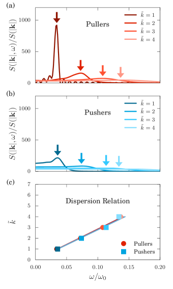
Figure 4: The calculation results for the spherically averaged Dynamic Structure Factor (DSF) $S\left(\boldsymbol{k},\omega\right)$, where $\boldsymbol{k}=\frac{2\pi}{L}\tilde{\boldsymbol{k}}$ is the wave vector, and $\omega$ the angular frequency (normalized by $\omega_{0}=2\pi/t_{0}$, where $t_{0}=a/U_{0}$). The top two figures show the simulation results for the DSF of (a) pullers at $\alpha=0.5$, and (b) pushers at $\alpha=-0.5$. The bottom figure (c) shows the relation between wave vectors and the positions of the Brillouin peaks. Arrows in (a) and (b) show the positions of peaks.

Several articles have shown similar results; some are consistent with our findings, while others are not. Simha and Ramaswamy predicted, using a continuum model that active matter suspensions with polar order can show sound like propagation modesAditi Simha and Ramaswamy (2002). They mainly studied the propagation mode of a director field, but also showed that the concentration field can exhibit the same type of propagation. Ezhilan et al. studied a similar continuum model Ezhilan et al. (2013). They reported pushers show stronger instability in their concentration field, contrary to our results that pullers have much higher Brillouin-like peaks and are more likely to show density fluctuations. They employed a far-field approximation, therefore they did not consider the finite size of the particles or the full hydrodynamic interactions. In our study, we took into account the full hydrodynamic interactions and finite volume of the swimmers. This difference is likely the cause for the contradictory results. Alarcon and PagonabarragaAlarcon and Pagonabarraga (2013) reported the same kind of density fluctuations in bulk puller systems, using direct numerical simulations with the same model swimmer system. They focused on the flocking behavior in bulk systems, while we studied the behaviors in confinement, which makes the flocking more apparent, and also identified the pseudo-sound property of the systems.

In conclusion, we confirmed, using direct numerical simulations with full hydrodynamics, that swimmer dispersions confined between flat parallel walls can exhibit a traveling wave-like motion. Furthermore, this non-trivial collective behavior is mainly due to the pseudo-acoustic properties of the swimmers themselves, with a purely hydrodynamic origin. This kind of phenomenon cannot be expected in conventional passive colloidal dispersions, since such density fluctuations would be suppressed due to viscous dampingHess and Klein (2006). In future works, we will consider complex wall geometries, such as gear shaped objects Kaiser et al. (2012); Angelani et al. (2009) and circular systems Woodhouse and Goldstein (2012). Based on our current results, we expect that spherically shaped particles, without any apparent alignment interaction, can generate non trivial collective motion due solely to hydrodynamic interactions.

We thank Simon K. Schnyder for useful discussions. This work was supported by JSPS KAKENHI Grant Number 26247069 and also by a Grant-in-Aid for Scientific Research on Innovative Areas “Fluctuation & Structure” (No.26103522) from the Ministry of Education, Culture, Sports, Science, and Technology of Japan. We also acknowledge the supporting program for interaction-based initiative team studies (SPIRITS) of Kyoto University.

References

- Sokolov et al. (2007) A. Sokolov, I. S. Aranson, J. O. Kessler, and R. E. Goldstein, Physical Review Letters 98, 158102 (2007).
- Nash et al. (2010) R. W. Nash, R. Adhikari, J. Tailleur, and M. E. Cates, Physical Review Letters 104, 258101 (2010).
- Mishra (2014) S. Mishra, Journal Of Statistical Mechanics-Theory And Experiment 2014, P07013 (2014).
- Nadell et al. (2009) C. D. Nadell, J. B. Xavier, and K. R. Foster, FEMS Microbiology Reviews 33, 206 (2009).
- Laage (2006) D. Laage, Science 311, 832 (2006).
- Angelani et al. (2009) L. Angelani, R. Di Leonardo, and G. Ruocco, Physical Review Letters 102, 048104 (2009).
- Di Leonardo et al. (2010) R. Di Leonardo, L. Angelani, D. Dell’Arciprete, G. Ruocco, V. Iebba, S. Schippa, M. P. Conte, F. Mecarini, F. De Angelis, and E. Di Fabrizio, Proceedings of the National Academy of Sciences of the United States of America 107, 9541 (2010).
- Woodhouse and Goldstein (2012) F. G. Woodhouse and R. E. Goldstein, Physical Review Letters 109, 168105 (2012).
- Kaiser et al. (2012) A. Kaiser, H. H. Wennsink, and H. Löwen, Physical Review E 108, 268307 (2012).
- Kaiser et al. (2014) A. Kaiser, A. Peshkov, A. Sokolov, B. ten Hagen, H. Löwen, and I. S. Aranson, Physical Review Letters 112, 158101 (2014).
- Aditi Simha and Ramaswamy (2002) R. Aditi Simha and S. Ramaswamy, Physical Review Letters 89, 058101 (2002).
- Ezhilan et al. (2013) B. Ezhilan, M. J. Shelley, and D. Saintillan, Physics of Fluids 25, 070607 (2013).
- Rafaï et al. (2010) S. Rafaï, L. Jibuti, and P. Peyla, Physical Review Letters 104, 098102 (2010).
- Evans et al. (2011) A. A. Evans, T. Ishikawa, T. Yamaguchi, and E. Lauga, Physics of Fluids 23 (2011).
- Alarcon and Pagonabarraga (2013) F. Alarcon and I. Pagonabarraga, Journal of Molecular Liquids 185, 56 (2013).
- Li and Ardekani (2014) G. J. Li and A. M. Ardekani, Physical Review E (2014).
- Zöttl and Stark (2014) A. Zöttl and H. Stark, Physical Review Letters (2014).
- Chaté et al. (2008) H. Chaté, F. Ginelli, G. Grégoire, F. Peruani, and F. Raynaud, The European Physical Journal B 64, 451 (2008).
- Ohta and Yamanaka (2014) T. Ohta and S. Yamanaka, Progress of Theoretical and Experimental Physics 2014, 11J01 (2014).
- Lighthill (1952) M. J. Lighthill, Communications on Pure and Applied Mathematics 5, 109 (1952).
- Blake (1971) J. R. Blake, Journal of Fluid Mechanics 46, 199 (1971).
- Ishikawa and Pedley (2007) T. Ishikawa and T. J. Pedley, Journal of Fluid Mechanics 588, 437 (2007).
- Nakayama and Yamamoto (2005) Y. Nakayama and R. Yamamoto, Physical Review E 71, 036707 (2005).
- Kim et al. (2006) K. Kim, Y. Nakayama, and R. Yamamoto, Physical Review Letters 96, 208302 (2006).
- Nakayama et al. (2008) Y. Nakayama, K. Kim, and R. Yamamoto, The European Physical Journal E 26, 361 (2008).
- Molina et al. (2013) J. J. Molina, Y. Nakayama, and R. Yamamoto, Soft Matter 9, 4923 (2013).
- Hansen and McDonald (2008) P. J. Hansen and I. R. McDonald, Theory of Simple Liquids (Academic Press, New York, 2008), 3rd ed.
- Chaté et al. (2006) H. Chaté, F. Ginelli, and R. Montagne, Physical Review Letters 96, 180602 (2006).
- Hess and Klein (2006) W. Hess and R. Klein, Advances in physics 32, 173 (2006).