The ecology of dark matter haloes I:
The rates and types of halo interactions

Abstract

Interactions such as mergers and flybys play a fundamental role in shaping galaxy morphology. Using the Horizon Run 4 cosmological $N$-body simulation, we studied the frequency and type of halo interactions, and their redshift evolution as a function of the environment defined by the large-scale density, pair separation, mass ratio, and target halo mass. Most interactions happen at large-scale density contrast $\delta\simeq 20$, regardless of the redshift corresponding to groups and relatively dense part of filaments. However, the fraction of interacting target is maximum at $\delta\simeq 1000$. We provide a new empirical fitting form for the interaction rate as a function of the halo mass, large-scale density, and redshift. We also report the existence of two modes of interactions from the distributions of mass ratio and relative distance, implying two different physical origins of the interaction. Satellite targets lose their mass as they proceed deeper into the host halo. The relative importance of these two trends strongly depends on the large-scale density, target mass, and redshift.

1 Introduction

In a hierarchical $\Lambda$CDM universe, low-mass haloes form first and merge together into a more massive one through gravitational attraction. Interactions might prevail during the halo formation and evolution. Therefore, the star-formation activity and the morphology of galaxies are governed by the halo interactions.

The effects of interactions also depend on the environment. In dense environments like clusters, intracluster interactions can suppress star formation by multiple high-velocity galaxy interactions within the cluster (harassment, Moore et al., 1996) or by tidal stripping (Merritt, 1984; Byrd & Valtonen, 1990). In addition to gravitational interactions, hydrodynamics also plays an important role with ram pressure stripping (Gunn & Gott, 1972; Bekki, 2014; Cen, 2014). Starvation or strangulation strips the hot gas and quenches star formation on a larger time-scale (Larson et al., 1980; Cen, 2014). In particular, minor mergers have been shown to be an efficient way to quench star formation, both from theoretical (e.g., Mihos & Hernquist, 1994) and observational (e.g., Kaviraj, 2014a) work. On the other hand, mergers have thus been considered as one of the most efficient processes to shape galaxies, turning blue, star-forming, spiral galaxies into red, dead, elliptical ones (Toomre & Toomre, 1972; Larson & Tinsley, 1978).

The density–morphology dependence has been studied for decades. Rich clusters are dominated by a giant elliptical, and the fraction of ellipticals decreases with increasing radial distance (Oemler, 1974; Dressler, 1980; Postman & Geller, 1984). On the contrary, fields are dominated by blue galaxies (Gómez et al., 2003; Goto et al., 2003; Tanaka et al., 2004).

Park et al. (2008) found — from the SDSS DR4 — that galaxies located within the virial radius of their nearest neighbour tend to have the same morphology as their neighbour as their separation decreases, whereas if their separation is larger than the virial radius, the fraction of elliptical decreases with increasing separation. Subsequent studies at low redshifts (Park et al., 2008; Park & Choi, 2009), high redshift ($0.4\leq z\leq 1.0$ Hwang & Park, 2009) and low-density environment (Yadav & Chen, 2014) confirmed these results.

The Press & Schechter (1974) formalism — and its extensions (Bond et al., 1991) — enabled the study of the merger rate from dark matter only (e.g., Berrier et al., 2006; Fakhouri & Ma, 2008, 2009; Hester & Tasitsiomi, 2010; Genel et al., 2010) or hydrodynamic (Murali et al., 2002; Maller et al., 2006; L’Huillier et al., 2012; Kaviraj et al., 2014; Rodriguez-Gomez et al., 2015; Welker et al., 2015) cosmological simulations. However, the merger rate still varies by an order of magnitude between different models (Hopkins et al., 2010). Environmental studies from SAMs (e.g., Jiang et al., 2014) and $N$-body simulations (e.g., Fakhouri & Ma, 2009) have also shown an enhancement of the merger rate in high-density regions.

Observationally, the merger rate is usually estimated either from close-pair counts (Patton et al., 2002; Keenan et al., 2014; Robotham et al., 2014; López-Sanjuan et al., 2015) or by morphological signatures (Conselice et al., 2003), and converted through a merger timescale. However, this merger timescale depends on the mass ratio and the gas fractions, which may lead to uncertainties in the merger rate (e.g., Lotz et al., 2010a, b). Several studies have used visual inspection to study the morphology (Darg et al., 2010; Lintott et al., 2011; Kaviraj, 2014b).

$N$-body simulations of galaxy encounters have shown that violent mergers were able to turn spiral galaxies into elliptical ones, supported by the random motions of their stars (e.g., Toomre & Toomre, 1972; Barnes, 1988, 1992). The implementation of hydrodynamics showed that gravitational torques from the interacting pairs could bring gas to the centre of the galaxies (Barnes & Hernquist, 1991, 1996), leading to bursts of star formation (e.g., Mihos & Hernquist, 1996; Tissera et al., 2002; Di Matteo et al., 2007; Hayward et al., 2014).

However, not all interactions end in mergers. If the relative velocity of the interacting galaxies is high enough, they will not merge within a dynamical timescales. This class of interaction, referred to as flyby, has been less studied, although in the recent years its interest has been growing (e.g., Moreno, 2012; Sinha & Holley-Bockelmann, 2012; Tonnesen & Cen, 2012). At low redshifts on high mass scales, flybys becomes as frequent as, or even more frequent than mergers (Sinha & Holley-Bockelmann, 2012). Moreno (2012) used the Millennium simulation (Springel et al., 2005) to analyse interacting pairs that are closer than a fixed comoving distance $d_{\text{crit}}$ at some point of their existence. They found that 53% of pairs never merge for $d_{\text{crit}}={1}\,h^{-1}\mathrm{Mpc}$, while a lower $d_{\text{crit}}$ reduces this fraction. Therefore, difficulties arise in observational work, since a non negligible fraction of observed pairs might not be gravitationally bound (Sinha & Holley-Bockelmann, 2012; Tonnesen & Cen, 2012). The presence of a hot gaseous halo in late-type galaxies is also important for the gas transfer and the star formation rate during distant interactions (Hwang & Park, 2015).

A key factor in understanding galaxy evolution, is to understand which of these phenomena (close and distant encounters) dominates. Distant interactions are weaker than close ones, but occur more frequently. It is then important to determine which one is the most efficient at shaping galaxy morphology. In this study, we used the large Horizon Run 4 $N$-body simulation to study the environmental dependency of the interaction rate, regardless of their final stage (merger or flybys).

In § 2 we describes the set of simulations used in this work and introduce our definition of interaction and environment. Our results about the interaction rate are presented in § 3, and a study of the distance and mass ratio is performed in § 4. § 5 discusses our results. Finally, the conclusions are drawn in § 6.

2 Simulation and method

We present the Horizon Run 4 simulation used here in § 2.1, and detail the method we used to construct the halo catalogues in § 2.2. Interactions are defined in § 2.4 and § 2.3 describes the density calculation.

2.1 Simulations

We used the Horizon run 4 simulation (Kim et al., 2015) performed with a memory-efficient version of the GOTPM code (Dubinski et al., 2004; Kim et al., 2009; Kim et al., 2011), with a box size $L={3150}\,h^{-1}\mathrm{Mpc}$, and $N=6300^{3}$ particles. The simulation used second order Lagrangian perturbation theory (2LPT) initial conditions at $z_{\text{i}}=100$ and a WMAP5 cosmology $(\Omega_{\text{b}},\Omega_{\text{m}},\Omega_{\Lambda},h,\sigma_{8},n_{s})$ = (0.044, 0.26, 0.74, 0.72, 0.79, 0.96), yielding a particle mass of $m_{\text{p}}\simeq$9.02\text{\times}{10}^{9}$\,h^{-1}\mathrm{M}_{\odot}$. This starting redshift combined with 2LPT initial conditions, ensures an accurate mass function and power spectrum (L’Huillier et al., 2014).

2.2 Halo catalogues

We detected haloes from the simulated particle distributions using OPFOF, a MPI-parallel version of the friends-of-friends (FOF) algorithm (Davis et al., 1985), with a standard linking length of 0.2 mean particle separations, and the gravitationally-stable subhaloes with the PSB algorithm (Kim & Park, 2006), which are assumed to host galaxies. PSB structures identified in an FoF halo are considered satellite subhaloes, except the most massive one which is defined as the main halo hosting the main galaxy. In the following, haloes will indistinctly refer to main or subhaloes.

The virial mass $M_{\text{v}}$ of each subhalo is defined as the sum of the mass of its member particles. The virial radius $R_{\text{v}}$ is then defined by

$$R_{\text{v}} =\left(\frac{3M_{\text{v}}}{4\pi\Delta_{\text{c}}(z)\rho_{\text{c}}(z)}\right)^{1/3},$$ (1)

where the critical density is defined as

$$\rho_{c}(z) =3H^{2}(z)/(8\pi G),$$ (2)

and the critical overdensity at redshift $z$, $\Delta_{\text{c}}(z)$ is well described by the empirical Bryan & Norman (1998) fitting formula

$$\Delta_{\text{c}}(z) =18\pi^{2}+82x-39x^{2},$$ (3)

where

$$x =\Omega(z)-1=-\frac{\Omega_{\Lambda}}{\Omega_{\text{m}}(1+z)^{3}+\Omega_{\Lambda}}.$$ (4)

Note that this definition of the virial radius is in physical (not comoving) units. However, in the following, we will only use comoving distances, and we include the Hubble flow $H\mathbf{r}$ in the definition of the velocity.

We defined target haloes (T) as main or subhaloes with ${M}_{\mathrm{T}}>M_{\text{thresh}}$. We chose $M_{\text{thresh}}\equiv\,$5\text{\times}{10}^{11}$\,h^{-1}\mathrm{M}_{\odot}$, corresponding to the mass of 56 particles. This choice yields a mean halo separation of ${5.17}\,h^{-1}\mathrm{Mpc}$, corresponding to SDSS galaxies brighter than $M_{r}=-19.8$ (Choi et al., 2010). For the neighbour haloes (N), we limit our catalogue to main or subhaloes with mass ${M}_{\mathrm{N}}>q_{0}M_{\text{thresh}}$, with $q_{0}=0.4$, yielding a minimal number of particles of 23. The choice of $M_{\text{thresh}}$  and $q_{0}$ are important for the construction of our catalogues. A lower $M_{\text{thresh}}$ will result into a larger target catalogue, while a lower $q_{0}$ enables to probe larger mass ratios. We then chose $q_{0}=0.4$ as a good trade-off, yielding $M_{\text{thresh}}=$5\text{\times}{10}^{11}$\,h^{-1}\mathrm{M}_{\odot}$. The mean separation of haloes in the neighbour catalogue is ${3.97}\,h^{-1}\mathrm{Mpc}$ at $z=0$, corresponding to that of SDSS galaxies brighter than $M_{r}=-18.7$ (Choi et al., 2010). Note that the target catalogue is a subsample of the neighbour catalogue. The minimal number of particles in the PSB subhaloes is set to 20, yielding a minmal mass of $$1.8\text{\times}{10}^{11}$\,h^{-1}\mathrm{M}_{\odot}$, therefore our neighbour catalogue is complete. The target (neighbour) catalogue contains $225\,406\,978$ ($472\,635\,985$) haloes at $z=0$. Note that we only consider the nearest neighbour, and ignore the effects of a second neighbour, which may become important for satellite pairs in clusters (Moreno et al., 2013). We discuss this choice in § 5.1

2.3 Quantification of the environment: large-scale density and distance to the nearest neighbour

The environment may be a key factor to define the interaction rate. Both large-scale and local environment have been shown to affect galaxy interactions. Muldrew et al. (2012) compared different ways to define the environment: using a fixed aperture or the distance to the $n$th nearest neighbour.

Another way to define and quantify the environment is to compute the eigenvalues of the smooth tidal field (Forero-Romero et al., 2009) or velocity-shear field (Hoffman et al., 2012).

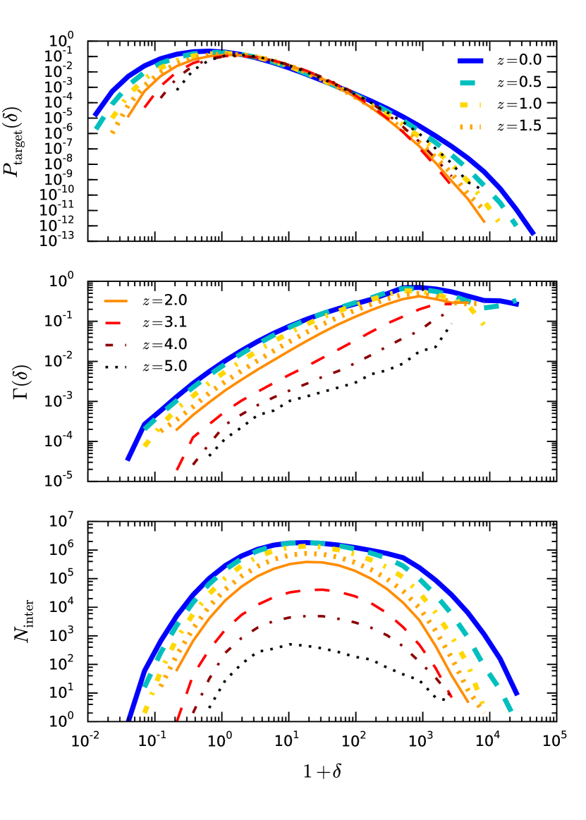
Figure 1: Top: Distribution of the large-scale background density at the location of the target haloes at different redshifts. Middle: Fraction of target haloes that encounter an interaction as a function of the large-scale environment $\delta$. Bottom: Histogram of interactions per density bin.

We defined the background density as in Park et al. (2007) and Park et al. (2008), by

$$\rho_{20}\equiv\sum_{i=1}^{20}M_{i}W(r_{i},h),$$ (5)

where $r_{i}$ and $M_{i}$ are the distance and mass of the $i$th closest galaxy in the catalogue, and $W$ is the SPH spline kernel (Monaghan & Lattanzio, 1985) of smoothing length $h$. The latter is searched to enclose 20 neighbours, which has been shown to be the smallest number yielding an accurate estimate of the density (Park et al., 2007). The adaptive nature of this technique enables to accurately probe the density both in high- and low-density regions (Park et al., 2007). Appendix A shows the relation between $\delta$ and the cosmic web.

Given the large number of haloes, we adopted a set of oct-sibling trees build in rectangular grids over the entire volume to efficiently compute the density, similar to Dubinski et al. (2004).

The local density is defined by the mass of the nearest neighbour and the separation $r$:

$$\rho_{\text{n}}\equiv\frac{3{M}_{\mathrm{N}}}{4\pi r^{3}}=\frac{\Delta_{\text{c}}\rho_{\text{c}}}{p^{3}},$$ (6)

and is thus fully described by the ratio of the pair separation to the virial radius of the neighbour at a given redshift $p\equiv d/R_{\text{vir,n}}$.

The mean density is the total mass of the haloes in the Neighbour catalogue

$$\bar{\rho}=\frac{1}{V}\sum{M_{i}}.$$ (7)

This enables us to normalise the density at different redshift by considering

$$\delta=\frac{\rho_{20}}{\bar{\rho}}-1.$$ (8)

We find $\bar{\rho}(z=0)=2.51\times 10^{10}\,h^{2}\,\mathrm{M}_{\odot}\,\mathrm{Mpc}^{-3}$.

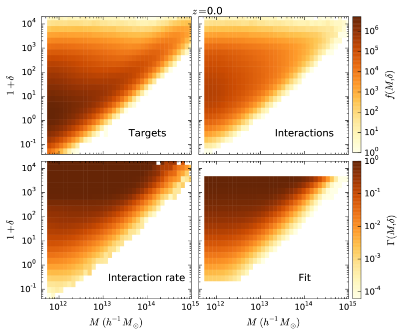
(a) $z=0$

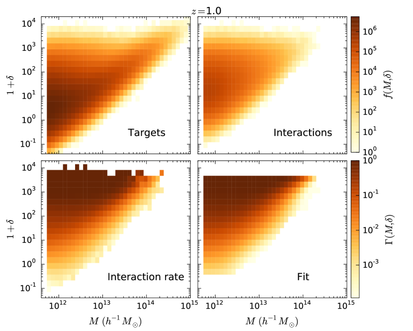
(b) $z=1$

Figure 2: Distribution function of the target haloes (top left) and interacting target (top right) as a function of the mass and large-scale density at $z=0$ (2(a)) and 1 (2(b)). Bottom left: interaction rate as a function of the mass and large-scale density. Bottom right: fit to the interaction rate with eq. (10).

2.4 Definitions of interactions

We define interacting systems as target haloes with mass ${M}_{\mathrm{T}}\geq M_{\text{thresh}}$ located within the virial radius of a neighbour more massive than $q_{0}{M}_{\mathrm{T}}$. Such target haloes are considered to be gravitationally influenced by their neighbour.

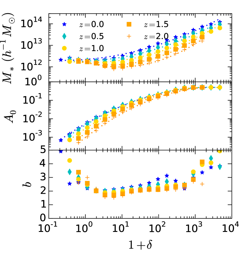
Figure 3: Dependence of the parameters $A_{0},M_{*}$, and $b$ of equation (10) on $\delta$ and $z$.

We define the interaction rate as the fraction of targets that are undergoing an interaction over the total number of target haloes. This definition slightly differs from some authors, who define the merger rate as the number of merger events per descendant (e.g., Fakhouri & Ma, 2008, 2009, 2010). Indeed, one can notice that an interaction may be counted twice if the mass ratio between two neighbours is between $q_{0}$ and $1/q_{0}$, and if their separation is smaller than both virial radii (which is likely to happen, since the virial radii of these two haloes are comparable).

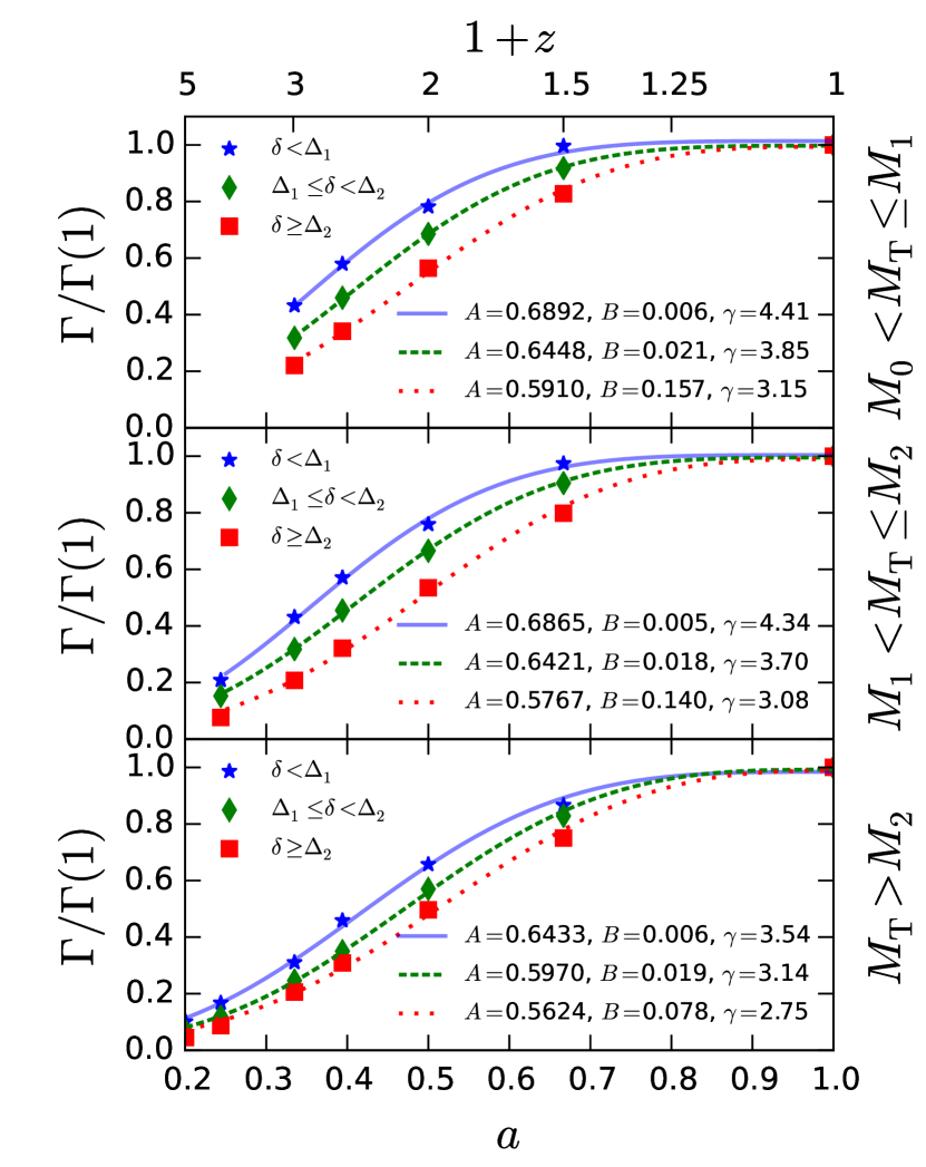
Figure 4: Interaction rate (normalised to the final value) as a function of the scale factor $a$ for low- (top), intermediate- (middle), and high-mass (top) bins, and for low- (stars), intermediate (diamonds), and high-density (squares), and the associated fit.

We will focus on several quantities: the mass of the halo, its background density, the mass ratio $q={M}_{\mathrm{N}}/{M}_{\mathrm{T}}$ and $p$ the pair separation divided by the virial radius of the neighbour. We also note that, in our definition, the mass ratio $q$ of the interaction is by definition larger than $q_{0}$, and the target halo can be the satellite ($q>1$) or the main halo ($q<1$). Our interaction rate corresponds to interaction rate per descendant only in the case $q>1$.

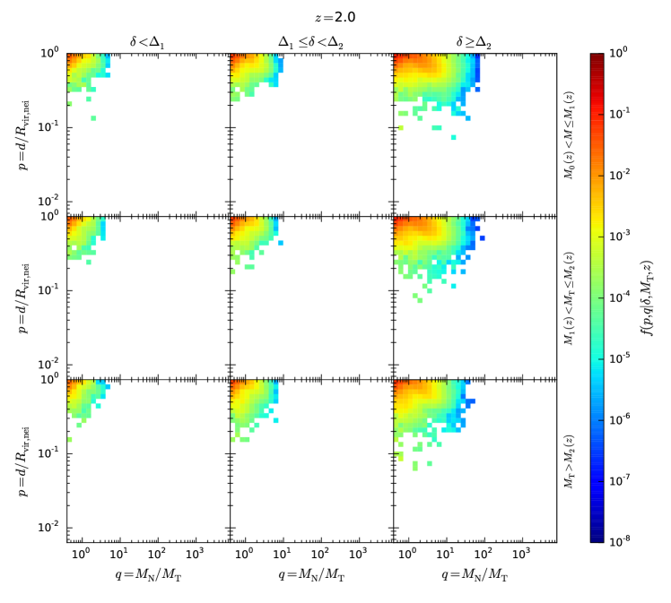
Figure 5: Probability distribution function $f$ as a function of the reduced distance $p=d/R_{\mathrm{vir,N}}$ and mass ratio $q={M}_{\mathrm{N}}/{M}_{\mathrm{T}}$ at $z=2$. The three columns are low-density ($\delta<\Delta_{i,1}$), medium-density ($\Delta_{i,1}\leq\delta<\Delta_{i,2}$), and high-density ($\delta\geq\Delta_{i,2}$) environments. The three rows are low-mass ($M_{0}<M<M_{1}$), intermediate-mass ($M_{1}<M<M_{2}$), and massive (${M}_{\mathrm{T}}\geq M_{2}$) target haloes.

Since our parameter space has 5 dimensions, we divide the whole target catalogue into subsamples according to the density, target mass, and redshift. We the study the two-dimensional $(p,q)$ distribution

$$\mathrm{d}^{2}N=f(p,q|\delta,{M}_{\mathrm{T}},z)\,\mathrm{d}p\,\mathrm{d}q,$$ (9)

where $\mathrm{d}^{2}N$ is the number of interactions in the interval $(p,p+\mathrm{d}p)$, $(q,q+\mathrm{d}q)$ at fixed redshift $z$, background density $\delta$, and halo mass ${M}_{\mathrm{T}}$.

3 Results

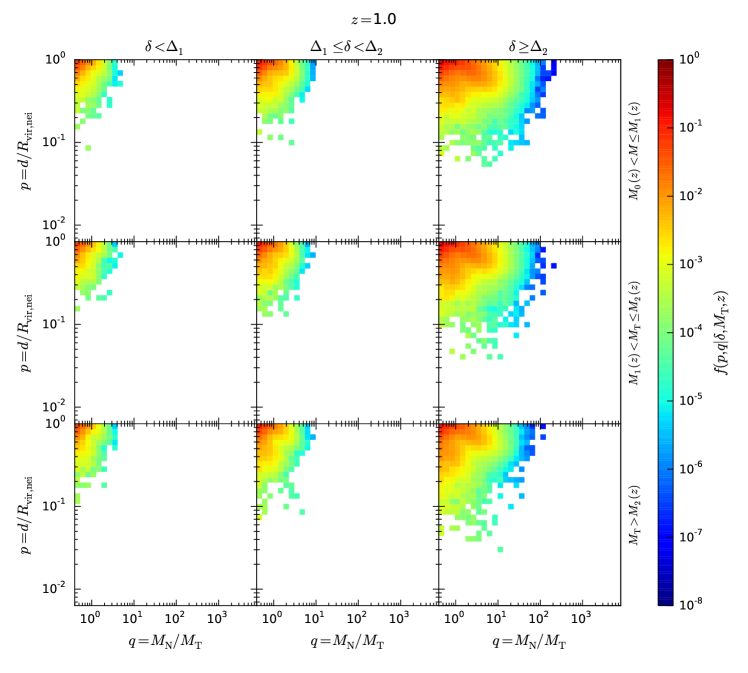
Figure 6: Same as Fig. 5, at $z=1$.

3.1 Mass and density dependence of the interaction rate

In this subsection, we are interested in the frequency of interactions that fulfil our definition that a target halo should be located within the virial radius of its neighbour.

The upper panel of Figure 1 shows the probability distribution of the large-scale density $\delta$ for all target haloes at different redshifts. The distribution range of $\delta$ becomes wider with decreasing redshift, reflecting the cosmic evolution of the large-scale structures. The distribution peaks at $\delta$ of a few units, and the peak height slightly diminishes with redshift.

The middle panel shows the fraction $\Gamma(\delta)$ of target haloes undergoing interactions as a function of the large-scale density $\delta$. In low-density regions, and at all redshift, this fraction is very low, while in high density regions ($\delta>100$), the fraction monotonously rises to reach a maximum at $1+\delta\simeq 500$, and then drops again. However, at these very-high densities, the number of targets is much lower, thus the statistical significance of the drop decreases. The interaction rate at a fixed density dramatically increase from $z=5$ to 2, and then shows little time evolution after this period.

Finally, the bottom panel of the figure shows the actual number of interactions. For all $\delta$, the number of interactions increases with decreasing redshift. We find that halo-halo interactions occur most frequently in the moderately high-density regions with a very narrow density range of $10<\delta<30$ at all studied redshifts. Therefore, even though halo interactions occur in a wide range of density environments, the majority of interacting haloes are always located in the regions with $\delta\simeq 20$. This corresponds to haloes in filaments (see Fig. 11).

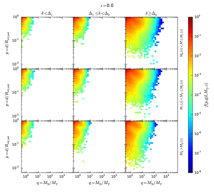
Figure 7: Same as Fig. 5, $z=0$.

Taking advantage of our unprecedented catalogue, we can study the interaction rate as a function of the mass $M$, background density, and redshift separately.

The upper-left panel of Fig. 22(a) and 2(b) show the distribution function of target haloes at $z=0$ and 1 as a function of the mass and large-scale density. This can be seen as an extension of the mass function on a two-dimensional plane. Most targets are located at intermediate densities and low masses. At low densities, only low-mass haloes are found, while at higher densities, the range of masses increases. It should be noted that the mass function has a double peak at fixed density. At very high $\delta$, however, the mass function is almost flat. The trend of increasing target mass with increasing density is due to host haloes, that follow the large-scale environment, while the wide range of masses at a given density is due to the subhaloes. Even though the definitions of environment are different, we find a qualitatively very similar distribution to Zhao et al. (2015) and Fakhouri & Ma (2009). The former studied the two-dimensional distribution of haloes in the density–$V_{\text{max}}$ plane, where the maximum velocity $V_{\text{max}}$ is a proxy for the halo mass. Our correlation between mass and density agree with their results. In the latter case, our results are closer to the left panel ($\delta_{7}$), that also includes the mass of the target halo.

The upper-right panel in each subfigure shows the distribution of interacting targets. Its shape follows closely that of the targets, except for the high-mass end at each density. This is because of our definition of interactions: the most massive haloes without a comparable neighbour are not considered to be interacting. Therefore, the double peaks in the mass function disappears.

The lower-left panels of Fig. 22(a) and 2(b) show the interaction rate, defined as the fraction of target that are interacting for a given mass and large-scale density. It is by definition proportional to the ratio of the upper-right to the upper-left panels. The rate at a given mass increases with increasing $\delta$, and reaches a plateau at high densities. At fixed density, the interaction rate is constant then drops towards large masses.

At higher redshifts, the distributions look very similar, but extend to lower masses and densities.

We proceeded in the following way to fit the interaction rate $\Gamma(M|\delta,z)$. At fixed $(\delta,z)$, we used an empirical function defined by

$$\Gamma(M|\delta,z)=A_{0}\,\mathrm{erfc}\left(b\log_{10}\left(\frac{M}{M_{*}}\right)\right),$$ (10)

where $A_{0},M_{*}$, and $b$ are free parameters depending on the large-scale density $\delta$ and the redshift. These parameters respectively describe the total interaction fraction, the characteristic mass at which the fraction drops, and the speed of the drop. This function was selected to reflect the plateau–drop shape of $\Gamma(M|\delta)$. We remove the lower and upper density bins that are almost empty of interactions, and for which the statistics are very poor.

We then show the resulting two-dimensional fit of $\Gamma(M,\delta)$ in the lower-right panel of Fig. 22(a) and 2(b). The fit is overall satisfactory, with an underestimation of the rate in the high-$\delta$ end of the range.

Figure 3 show the dependence of the parameters $M_{*},A_{0}$, and $b$ on the large-scale density at each redshift. We fit them with a second-order polynomial in $\log_{10}(1+\delta)$, and show it as a dotted line.

3.2 Time evolution of the interaction rate

In this section, we focus on the time evolution of the interaction rate. In order to follow the same biased objects in a statistical sense, we proceeded as follows. At a fixed redshift, we divided our sample of target halo into subsamples of equal number of targets, constant at all redshifts, according to their mass. Then, we divided each mass-subsample into three subsamples according to the large-scale density of the targets. In practice, at $z=4$, we selected all target haloes more massive than $M_{2}(z=4)\equiv$8.67\text{\times}{10}^{11}$\,h^{-1}\mathrm{M}_{\odot}$, corresponding to $N_{0}\simeq$4.9\text{\times}{10}^{6}$$. We then divided this sample into three subsamples of the same size in terms of the number of target halos, namely, $\delta<\Delta_{2,1}(z=4)$, $\Delta_{2,1}(z=4)<\delta<\Delta_{2,2}(z=4)$, and $\delta>\Delta_{2,2}(z=4)$. At $z=3.1$, we found $M_{2}(z=3.1)$ and $M_{1}(z=3.1)$ such that we have two subsamples according to the target mass, with the same number of targets as at $z=4$. We then divided them into three subsamples according to the target large-scale density. At lower redshift, we introduced another subsamples at low masses, $M_{0}(z)<M<M_{1}(z)$. This ensures that the number of targets in each bin of mass and density is constant, about 1.6 millions, and thus that we are following statistically similar haloes across different redshifts. The redshift-evolution of $M_{i}$ and $\Delta_{j,i},(i\in\{0,1,2\},j\in\{1,2\})$ is shown in Fig. 13.

Figure 4 shows the redshift-evolution of the interaction rate for low- (top), intermediate- (middle), and high-masses (bottom panel). The low-, intermediate-, and high-density bins are shown as stars, diamonds, and squares. For visualisation sake, we normalised the rates to be 1 at $a=1$. We fit the interaction rate as follow:

$$\Gamma(a)=B\,\text{exp}\left(\left(-\frac{1-a}{A}\right)^{\gamma}\right),$$ (11)

and the values of $A,B$, and $\gamma$ in each bin are shown in the figure. The resulting fit is shown as a dotted line for each subsample. $\Gamma$ has an inflexion point at $a=1-A((\gamma-1)/\gamma)^{1/\gamma}$, which may be seen at $a\simeq 0.3$ – 0.4. It is worth noting that this fitting function is able to reproduce the behaviour of the interaction rate from $a=0.2$ to 1 and for all range of mass and density considered. Note that the fitting function is still positive at $a=0$, so the description is not perfect at very low $a$, but is good enough for the range of redshifts of interest. The actual value of the interaction rates can be directly read from $B$. The shapes are very similar, rising then reaching saturation, but the mass and density dependencies can be seen. At fixed mass, the slope is steeper in the high-density bin, and the rate in the low-density bin is flatter, showing an earlier saturation. The final interaction rate significantly ($B$) grows with the density, while $A$ slowly decreases with increasing density. At fixed density bin, the slope becomes shallower and the interaction rate drops toward larger masses. This counter-intuitive point was already seen in the right panels of Fig. 2, where the interaction rate drops at large masses, and is due to our definition of interactions. Also, the raise is somewhat delayed in the largest mass bin. $a_{1/2}$, the time when the interaction rate reaches half of its final value, is larger in this bin.

4 Type of interactions

After studying the effects of the mass and environments on the interaction rate, we study further to investigate the distributions of $p$ and $q$.

4.1 Distribution of the distance and mass ratio of interactions

Figure 5, 6, and 7 show the distribution $f(p,q|\delta,{M}_{\mathrm{T}},z)$ at $z=2$, 1, and 0, in the same bins of density and target halo mass as in § 3.2. The function is normalised in each bin such that

$$\int\!f(p,q)\,\mathrm{d}p\,\mathrm{d}q=\frac{N_{\text{inter, bin}}}{N_{\text{target, bin}}}$$ (12)

over the integration domain, where $N_{\text{inter, bin}}$ and $N_{\text{target, bin}}$ are the number of interactions and targets in each bin. Note that by construction, $N_{\text{target, bin}}$ is constant in each panel. The distribution function is thus normalised to the interaction rate in the bin, as defined in § 3 and Fig. 2. There is a clear dependence on the halo mass and on the background density.

One can also see in the lower right panel the existence of two main branches: a vertical branch at $q\lesssim 1$ and an oblique branch. They correspond to different stages of interactions:

1. [(i)]

2. The vertical branch, with a large range of $p$ for $q\simeq 1$,

3. The oblique branch, where the mass ratio increases as the separation becomes smaller. This branch can be understood as tidal stripping as the satellites orbits closer and closer to the centre of the main halo (e.g., Sales et al., 2007).

Interestingly, the target mass and background density have a strong influence on the relative importance of both branches.

At fixed redshift and mass bin, increasing the density has two main effects. First, the range of $q$ becomes larger at higher densities. This reflects the fact that massive haloes are located in high-density regions. The second effect, that directly follows from the first one, is that branch (ii) is shifted towards larger values of $q$.

When the redshift and the density bins are fixed, going towards higher masses increases the importance of branch (i). Moreover, since the target becomes more massive, its virial radius increases, and the minimal value of $p$ decreases.

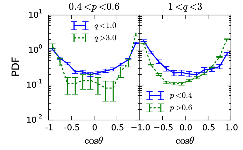
Figure 8: Distribution of $\cos\theta$ for the different subsamples. $\theta$ is the angle of the neighbour’s velocity vector from the position vector from the target.

Finally, at fixed mass and density bin, there is also a redshift dependence. Since haloes become more massive, the total range of $q$ becomes larger. The importance of branch (ii) fades away with decreasing redshift, while branch (i) becomes more and more important.

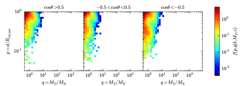
Figure 9: Interaction rate as a function of $(p,q)$ for interactions with $\cos\theta>0.5$ (left), $-0.5<\cos\theta<0.5$ (middle), and $\cos\theta<-0.5$ (right).

We interpret these two branches as follows: As the interaction starts, the satellite halo (less massive one) enter within the host, and as it proceeds towards the centre, loses its mass through tidal stripping (branch (ii)). After the closest approach, the satellite can be anywhere within the neighbour, corresponding to branch (i). In the next section, we focus on understanding the physics of these two branches.

4.2 A closer look at the branches

In order to better understand the physical meaning of these two branches, we now focus on the intermediate-density, high-mass panel of Fig 7. We consider all interactions with $0.4<p<0.6$ and separate then between low- ($q<1$, the target is the host of its neighbour) and high-$q$ values ($q>3$), and now focus on $\theta$, the angle between the position and the velocity of the neighbour with respect to the target, for the two subsamples. Tangential orbits have $\cos\theta=0$, while receding (approaching) radial orbits have $\cos\theta=(-)1$.

The left panel of Fig. 8 shows the distribution of $\cos\theta$. For a pure random case, the distribution of $\cos\theta$ should be flat. Interactions with $q<1$ have a flatter distribution of $\cos\theta$, reflecting a larger amount of tangential orbits than those with $q>3$. It can be seen that the distribution of $\cos\theta$ for interactions with $q<1$ is flatter, hence more random. Therefore, the branch at the left of the $p-q$ plane corresponds to the haloes whose orbits are randomised after they envounter and orbit around their neighbour. On the other hand, the interactions with $q>3$ have significantly fewer tangential orbits compared to the random case. This means that the upper right branch in the $p-q$ plane is composed of haloes in the course of the first encounter in radial orbits.

The right panel of Fig. 8 shows, for a fixed range of neighbour-to-target mass ratio of $1<q<3$, the distributions for $p<0.4$ (solid line) and $p>0.6$ (dotted line). Interaction with $p<0.4$, which belong to the left branch in the $p-q$ plane, show more consistency with random orbits. The interactions with $p>0.6$ show relative scarcity of tangential orbits with some excess of receding radial orbits over approaching orbits. These observations reinforces the conclusion that the left branch is formed by relaxed haloes.

Figure 9 shows $f(p,q|z=0,\Delta_{1,2}<\delta<\Delta_{2,2},M>M_{2})$, the middle panel of the third row of Fig. 7, for $\cos\theta>0.5$ (left), $-0.5<\cos\theta<0.5$ (middle), and $\cos\theta<-0.5$ (right). One can see that the left and right panels, corresponding to receding and approaching radial orbits respectively, have a prominent upper right branch, while the middle row, corresponding to tangential orbits, shows fewer interactions in this locus. This again reflects the fact that branch (ii) consists of haloes undergoing their first encounter, with a rather radial orbit, while branch (i) consists of haloes that have already experienced many close encounters.

5 Discussion

5.1 Choice of the neighbour

In this section, we study the influence of the choice of the neighbour to define interactions. Park et al. (2008) tested the neighbour with the largest tidal energy deposit (LTED) as the most influential neighbour, and found essentially no difference. For galaxies in the field, this makes very little difference since the closest neighbour is more likely to be the only one affecting the target. The situation may be different in high-density regions, where two satellite may be interacting while the main halo, even more distant, may have a stronger influence (Moreno et al., 2013). Park & Hwang (2009) showed that while the structural parameters (e.g., concentration) depends on the clustercentric distance, the star formation history is still a function of the closest neighbour.

Following Park et al. (2008), we computed the energy deposit by each of the 20 neighbours used to compute the large-scale density, provided that it fulfils the conditions (${M}_{\mathrm{N}}>q_{0}{M}_{\mathrm{T}}$ and $r<R_{\text{vir,N}}$) using Binney & Tremaine (2008):

$$\Delta E\propto\frac{{M}_{\mathrm{N}}^{2}a^{2}}{\Delta v^{2}(a^{2}+R_{\text{vir,N}}^{2})^{2}},$$ (13)

where $a$ is the rms radius of the target halo, and $\Delta v$ the relative velocity. Note that we used the virial radius of the target $R_{\text{T}}$ rather than the rms radius, but we expect the results to be unchanged. We then defined the neighbour with the largest $\Delta E$ as the most influential neighbour.

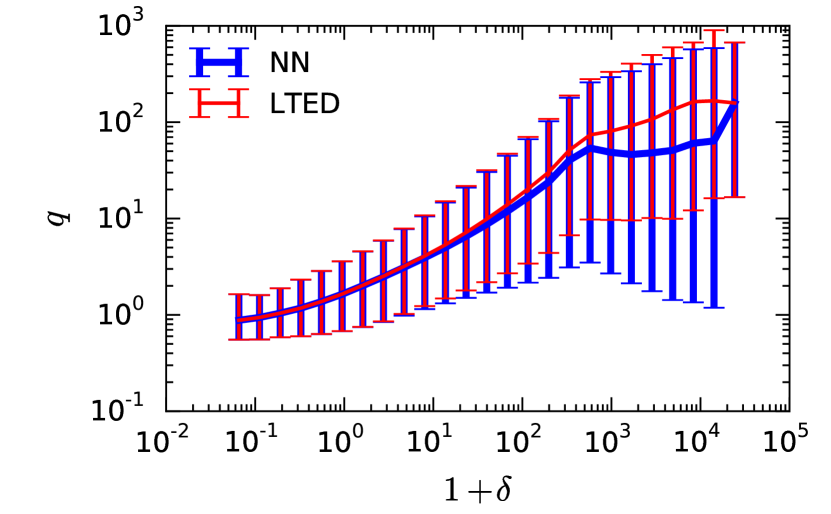
Figure 10: Effect of the definition of the neighbour. Shown are the median value and the 15th and 85th percentiles of the mass ratio $q$ for each density bin for the default nearest neighbour case (thick blue lines, NN), and for the maximal energy deposit (red line, LTED).

Fig. 10 shows the median of the mass ratio $q$ in each bin of density. Interactions using the nearest neighbour (NN) are shown in red, thick lines, and the LTED case is shown in blue line. The error bars show the 15th and 85th percentiles. As expected, the median of the mass ratio increases at larger densities since it is more likely to find a more massive neighbour. Up to $\delta\simeq 500$, the choice of the neighbour has no effect. At higher densities, as expected, the neighbour with the LTED is not necessarily the NN, but more likely to be a more massive halo, which leads to larger mass ratios. Since most interactions occur at rather low densities, $\delta$ of a few tens, the choice of the neigbhbour has no effect. However, if one is interested in interactions within clusters, one should define the neigbhour carefully.

5.2 Comparison with previous work

Previous theoretical work from simulations (e.g., Fakhouri & Ma, 2008, 2009; Genel et al., 2010) studied the merger rate per time unit using merger trees, and typically found a merger rate of $\mathrm{d}{N_{\text{merg}}/\mathrm{d}t}\propto(1+z)^{\alpha}$, while Fakhouri & Ma (2009) found an environmental factor $(1+\delta_{7})^{\beta}\left(M/{M_{12}}\right)^{\gamma}$, where $\delta_{7}$ is the local density computed over a sphere of radius ${7}\,h^{-1}\mathrm{Mpc}$. However, our approach differs from previous theoretical studies in that we do not use merger trees to define interactions, but rather look at the distance to the closest neighbour at a given time. This makes direct comparison with previous work difficult. Indeed, in our approach, the same interaction may be counted at different redshifts, while in other studies it will only be counted when the merger is complete.

Our approach is by construction closer to observations in that we look at the instantaneous interaction fraction, namely, the fraction of target that are undergoing an interaction at a given redshift, corresponding to $f_{\text{m}}$ in (Lotz et al., 2008). However, our condition that the target should lie within the virial radius of its neighbour, increases our interaction numbers especially at low-redshifts where the physical virial radius of the studied mass range is typically 0.5 to ${1}\,h^{-1}\mathrm{Mpc}$, compared to close-pair counts that limit the separations to a few ${10}\,h^{-1}\mathrm{kpc}$.

The main advantage of our approach, besides its simplicity, is that it does not require observations to use a merger timescale, that can be a source of uncertainty. Instead, the observed merger fraction can be directly compared to our fitting formulae. However, one should keep in mind that, since we consider distant interactions, our pair separation can be larger than the typical ${30}\,h^{-1}\mathrm{kpc}$ separation used to calculate merger rates.

Observationally, most studies define the interaction radius, i.e., the largest radius to define an interacting pair, as fixed in physical scales. López-Sanjuan et al. (2015) compiled several study of close pairs for $0<z<1.2$, with a minimal projected separation of ${100}\,h^{-1}\mathrm{kpc}$ (physical), and fitted an interaction fraction of $f=f_{0}(1+z)^{m}$. They found that $f_{0}$ decreases and $m$ increases with decreasing magnitude cut. While our fitting formula are different, $f_{0}$ and $m$ can be related to our $B$ and $\gamma$ parameters. However, their behaviours are quite different, since $B$ is constant with mass, except in the largest density bin. The main difference with our approach is the use of a fixed projected radius for the definition of interacting pairs, while our interaction distance depends on the neighbour. At fixed mass, and in proper units, the virial radius increases with decreasing redshift (since $R_{\text{vir}}$ and $\Delta_{\text{c}}$ decrease, c.f. equations 1 and 3). Moreover, haloes also accrete mass, which also makes the virial radius grow. These considerations results in a larger interaction fraction at lower redshift in our definition.

6 Summary

In this study, we used the massive Horizon run 4 cosmological $N$-body simulation to investigate halo interactions, by considering three aspects of the environment, namely, internal (target mass), local (distance to the nearest neighbour), and large-scale (background density).

This simulation has the largest size among all simulations that have been used to study galaxy interactions, which enables to study the environment dependence and very good statistics, while its resolution is high enough to study haloes with masses down to $$5\text{\times}{10}^{11}$\,h^{-1}\mathrm{M}_{\odot}$. We defined target and neighbour haloes as haloes more massive than $5\text{\times}{10}^{11}$ and $$2\text{\times}{10}^{11}$\,h^{-1}\mathrm{M}_{\odot}$, and we define a target of mass ${M}_{\mathrm{T}}$ to be interacting if it is located within the virial radius of a neighbour more massive than $0.4{M}_{\mathrm{T}}$.

Our findings are summarised as follow:

• Interactions preferentially occur at intermediate large-scale background densities, $\delta\simeq 20$, regardless of the redshift, and for targets more massive than $$5\text{\times}{10}^{11}$\,h^{-1}\mathrm{M}_{\odot}$. The interaction rate, i.e.,   the fraction of targets undergoing an interaction, reaches its maximum at larger values: $\delta\simeq 1000$.

• We propose a new functional fit (eq. 10) for the interaction rate as a function of the target mass and large-scale background mass density at fixed redshift, and give the redshift-evolution of the fit parameters.

• The interaction rate as a function of time has a universal shape, rising and saturating. We propose a fitting formula for the time evolution of the interaction rate (eq. 11). This function strongly depends on the large-scale density and target mass. Larger density yield a steeper slope and larger final interaction rate, and massive haloes saturate later.

• We reported the existence of two branches in the two-dimensional distribution $f(p,q|\delta,{M}_{\mathrm{T}},z)$, namely: an oblique branch where the distance to the neighbour decreases as the mass ratio increases, reflecting the loss of the satellite mass through tidal stripping as it orbits within the main halo. A second branch at lower $p$ for the same $q$ corresponds to interactions that already passed the closest approach and whose orbits became randomised.

• The relative importance of the two trends strongly depend on the large-scale density, target mass, and redshift.

In a paper in preparation, we will study the effects of interactions on parameters such as the alignment of the spin and major axes of the interacting haloes, and their orbits. In a next step, we will add hydrodynamics to study the galaxy (rather than the halo) interaction rate, which can be significantly different (Hopkins et al., 2010), and to probe the effects of gas physics on the morphological transformation of galaxies.

We argue that observers may use our definitions to measure the interaction fraction. In a next paper, we plan to apply our method to publicly available observational data in order to compare the evolution of interaction fraction between observations and our theoretical results.

Acknowledgements

We thank KIAS Center for Advanced Computation for providing computing resources. We thank the anonymous referee for her/his precious comments that helped improving this manuscript.

Appendix A $\delta$ and the cosmic web

It is interesting to understand the relation between the overdensity parameter $\delta$ and the cosmic web, namely, where haloes with a given $\delta$ are located within the cosmic web. Figure 11 shows a $150\times 150\times 20$${}\,h^{-1}\mathrm{Mpc}$ slice at $z=0$ (top) and 1 (bottom). High-$\delta$ haloes are shown in large, red circles, intermediate-$\delta$ ($10<1+\delta<30$) in medium, cyan circles, while other haloes are shown in small, blue circles. Haloes are overplotted on top of the density map computed with the Triangular-Shape Clouds, with a pixel size of ${0.5}\,h^{-1}\mathrm{Mpc}$, the same as used for the PM calculation. At $z=0$, haloes with $\delta>100$(red) can be found in nodes, while intermediate ($10<\delta<30$) are found in filaments. On the other hand, at $z=1$ the overall density fluctuation amplitude is lower, and the haloes with $\delta>100$ are located only in the rarer highest density nodes. Since we vary the density threshold to cope with the evolution of the growth factor, the type of environment corresponding to each density bin is supposed to be independent of redshift. We conclude that the overdensity $1+\delta$ is a good proxy for the environment.

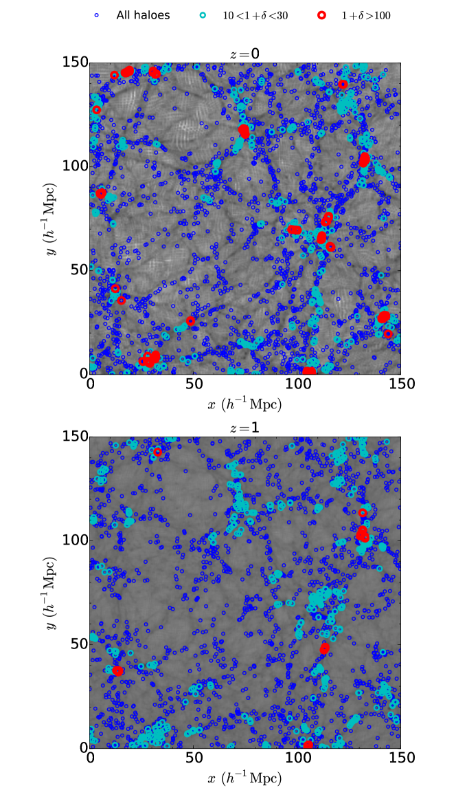
Figure 11: Distribution of haloes with different overdensities in the cosmic web at $z=0$ (top) and 1 (bottom). The grey background is the density field computed over ${0.5}\,h^{-1}\mathrm{Mpc}$ pixels with a TSC method. The larger values (large red circles, $1+\delta>100$) are located in the nodes, while intermediate valuers (medium, cyan circles $10<1+\delta<30$) are located in the filaments.

Appendix B Effects of $M_{0},M_{1}$, and $M_{2}$

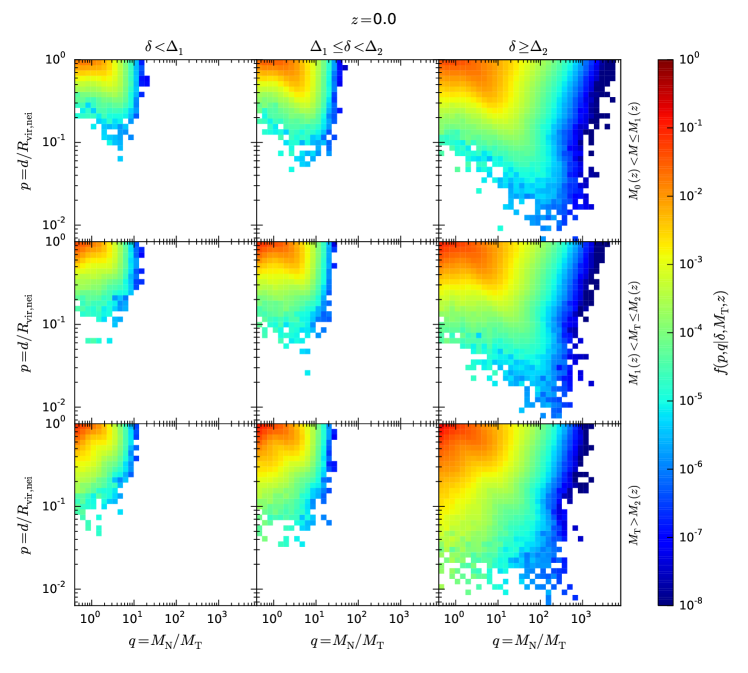
Figure 12: Same as Fig. 7, with $z_{\text{max}}=2$.

Fig. 12 is the same as Fig. 7, but using $z_{\text{max}}=2$ instead of 4. The larger number of targets available from $z=2$ enables us to keep better statistics, but prevents from doing a redshift-evolution study as in § 3.2. It results in a much higher number of targets in each panel, about 20 millions, from $z=2$ to 0.

The value of $M_{0},M_{1}$, and $M_{2}$ are respectively $6.86\text{\times}{10}^{11}$, $1.1\text{\times}{10}^{12}$, and $$2.14\text{\times}{10}^{12}$\,h^{-1}\mathrm{M}_{\odot}$, compared to $7.68\text{\times}{10}^{12}$, $1.10\text{\times}{10}^{13}$, and $$1.99\text{\times}{10}^{13}$\,h^{-1}\mathrm{M}_{\odot}$ for the $z_{\text{max}}=4$ (shown in Fig. 13) case, which implies that all targets in Fig. 7 are in the lower panel of Fig. 12, resulting in a more important oblique branch.

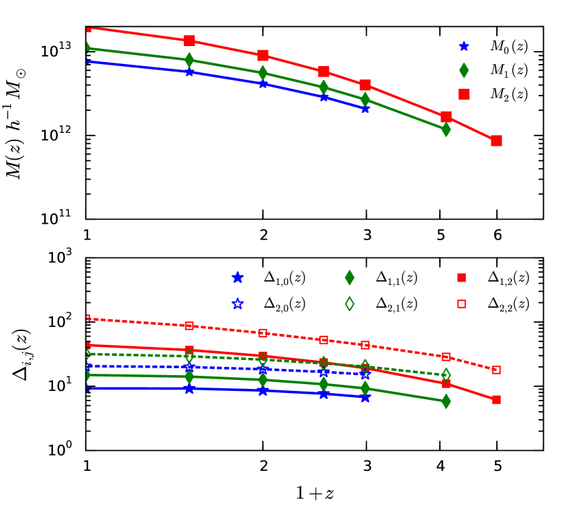
Figure 13: Redshift evolution of $M_{j}$ (top), and $\Delta_{i,j}$ (bottom), where $j$ stands for the mass bin and $i$ for the density bin, for the $z_{\text{max}}=4$ case in § 3.2.

References

- Barnes (1988) Barnes J. E., 1988, ApJ, 331, 699
- Barnes (1992) Barnes J. E., 1992, ApJ, 393, 484
- Barnes & Hernquist (1996) Barnes J. E., Hernquist L., 1996, ApJ, 471, 115
- Barnes & Hernquist (1991) Barnes J. E., Hernquist L. E., 1991, ApJ, 370, L65
- Bekki (2014) Bekki K., 2014, MNRAS, 438, 444
- Berrier et al. (2006) Berrier J. C., Bullock J. S., Barton E. J., Guenther H. D., Zentner A. R., Wechsler R. H., 2006, ApJ, 652, 56
- Binney & Tremaine (2008) Binney J., Tremaine S., 2008, Galactic Dynamics: Second Edition. Princeton University Press
- Bond et al. (1991) Bond J. R., Cole S., Efstathiou G., Kaiser N., 1991, ApJ, 379, 440
- Bryan & Norman (1998) Bryan G. L., Norman M. L., 1998, ApJ, 495, 80
- Byrd & Valtonen (1990) Byrd G., Valtonen M., 1990, ApJ, 350, 89
- Cen (2014) Cen R., 2014, ApJ, 781, 38
- Choi et al. (2010) Choi Y.-Y., Han D.-H., Kim S. S., 2010, Journal of Korean Astronomical Society, 43, 191
- Conselice et al. (2003) Conselice C. J., Bershady M. A., Dickinson M., Papovich C., 2003, AJ, 126, 1183
- Darg et al. (2010) Darg D. W., Kaviraj S., Lintott C. J., Schawinski K., Sarzi M., Bamford S., Silk J., Andreescu D., Murray P., Nichol R. C., Raddick M. J., Slosar A., Szalay A. S., Thomas D., Vandenberg J., 2010, MNRAS, 401, 1552
- Davis et al. (1985) Davis M., Efstathiou G., Frenk C. S., White S. D. M., 1985, ApJ, 292, 371
- Di Matteo et al. (2007) Di Matteo P., Combes F., Melchior A.-L., Semelin B., 2007, A&A, 468, 61
- Dressler (1980) Dressler A., 1980, ApJ, 236, 351
- Dubinski et al. (2004) Dubinski J., Kim J., Park C., Humble R., 2004, New A, 9, 111
- Fakhouri & Ma (2008) Fakhouri O., Ma C.-P., 2008, MNRAS, 386, 577
- Fakhouri & Ma (2009) Fakhouri O., Ma C.-P., 2009, MNRAS, 394, 1825
- Fakhouri & Ma (2010) Fakhouri O., Ma C.-P., 2010, MNRAS, 401, 2245
- Forero-Romero et al. (2009) Forero-Romero J. E., Hoffman Y., Gottlöber S., Klypin A., Yepes G., 2009, MNRAS, 396, 1815
- Genel et al. (2010) Genel S., Bouché N., Naab T., Sternberg A., Genzel R., 2010, ApJ, 719, 229
- Gómez et al. (2003) Gómez P. L., Nichol R. C., Miller C. J., Balogh M. L., Goto T., Zabludoff A. I., Romer A. K., Bernardi M., Sheth R., Hopkins A. M., Castander F. J., Connolly A. J., Schneider D. P., Brinkmann J., Lamb D. Q., SubbaRao M., York D. G., 2003, ApJ, 584, 210
- Goto et al. (2003) Goto T., Yamauchi C., Fujita Y., Okamura S., Sekiguchi M., Smail I., Bernardi M., Gomez P. L., 2003, MNRAS, 346, 601
- Gunn & Gott (1972) Gunn J. E., Gott III J. R., 1972, ApJ, 176, 1
- Hayward et al. (2014) Hayward C. C., Torrey P., Springel V., Hernquist L., Vogelsberger M., 2014, MNRAS, 442, 1992
- Hester & Tasitsiomi (2010) Hester J. A., Tasitsiomi A., 2010, ApJ, 715, 342
- Hoffman et al. (2012) Hoffman Y., Metuki O., Yepes G., Gottlöber S., Forero-Romero J. E., Libeskind N. I., Knebe A., 2012, MNRAS, 425, 2049
- Hopkins et al. (2010) Hopkins P. F., Croton D., Bundy K., Khochfar S., van den Bosch F., Somerville R. S., Wetzel A., Keres D., Hernquist L., Stewart K., Younger J. D., Genel S., Ma C.-P., 2010, ApJ, 724, 915
- Hwang & Park (2009) Hwang H. S., Park C., 2009, ApJ, 700, 791
- Hwang & Park (2015) Hwang J.-S., Park C., 2015, ApJ in press
- Jiang et al. (2014) Jiang C. Y., Jing Y. P., Han J., 2014, ApJ, 790, 7
- Kaviraj (2014a) Kaviraj S., 2014a, MNRAS, 440, 2944
- Kaviraj (2014b) Kaviraj S., 2014b, MNRAS, 437, L41
- Kaviraj et al. (2014) Kaviraj S., Devriendt J., Dubois Y., Slyz A., Welker C., Pichon C., Peirani S., Le Borgne D., 2014, arXiv:1411.2595
- Keenan et al. (2014) Keenan R. C., Foucaud S., De Propris R., Hsieh B. C., Lin L., Chou R. C. Y., Huang S., Lin J. H., Chang K. H., 2014, ApJ, 795, 157
- Kim & Park (2006) Kim J., Park C., 2006, ApJ, 639, 600
- Kim et al. (2009) Kim J., Park C., Gott III J. R., Dubinski J., 2009, ApJ, 701, 1547
- Kim et al. (2015) Kim J., Park C., L’Huillier B., Hong S. E., 2015, JKAS in prep.
- Kim et al. (2011) Kim J., Park C., Rossi G., Lee S. M., Gott III J. R., 2011, Journal of Korean Astronomical Society, 44, 217
- Larson & Tinsley (1978) Larson R. B., Tinsley B. M., 1978, ApJ, 219, 46
- Larson et al. (1980) Larson R. B., Tinsley B. M., Caldwell C. N., 1980, ApJ, 237, 692
- L’Huillier et al. (2012) L’Huillier B., Combes F., Semelin B., 2012, A&A, 544, A68
- L’Huillier et al. (2014) L’Huillier B., Park C., Kim J., 2014, New A, 30, 79
- Lintott et al. (2011) Lintott C., Schawinski K., Bamford S., Slosar A., Land K., Thomas D., Edmondson E., Masters K., Nichol R. C., Raddick M. J., Szalay A., Andreescu D., Murray P., Vandenberg J., 2011, MNRAS, 410, 166
- López-Sanjuan et al. (2015) López-Sanjuan C., Cenarro A. J., Varela J., Viironen K., Molino A., Benítez N., 2015, A&A, 576, A53
- Lotz et al. (2008) Lotz J. M., Davis M., Faber S. M., Guhathakurta P., Gwyn S., Huang J., Koo D. C., Le Floc’h E., Lin L., Newman J., Noeske K., Papovich C., Willmer C. N. A., Coil A., 2008, ApJ, 672, 177
- Lotz et al. (2010a) Lotz J. M., Jonsson P., Cox T. J., Primack J. R., 2010a, MNRAS, 404, 590
- Lotz et al. (2010b) Lotz J. M., Jonsson P., Cox T. J., Primack J. R., 2010b, MNRAS, 404, 575
- Maller et al. (2006) Maller A. H., Katz N., Kereš D., Davé R., Weinberg D. H., 2006, ApJ, 647, 763
- Merritt (1984) Merritt D., 1984, ApJ, 276, 26
- Mihos & Hernquist (1994) Mihos J. C., Hernquist L., 1994, ApJ, 425, L13
- Mihos & Hernquist (1996) Mihos J. C., Hernquist L., 1996, ApJ, 464, 641
- Monaghan & Lattanzio (1985) Monaghan J. J., Lattanzio J. C., 1985, A&A, 149, 135
- Moore et al. (1996) Moore B., Katz N., Lake G., Dressler A., Oemler A., 1996, Nature, 379, 613
- Moreno (2012) Moreno J., 2012, MNRAS, 419, 411
- Moreno et al. (2013) Moreno J., Bluck A. F. L., Ellison S. L., Patton D. R., Torrey P., Moster B. P., 2013, MNRAS, 436, 1765
- Muldrew et al. (2012) Muldrew S. I., Croton D. J., Skibba R. A., Pearce F. R., Ann H. B., Baldry I. K., Brough S., Choi Y.-Y., 2012, MNRAS, 419, 2670
- Murali et al. (2002) Murali C., Katz N., Hernquist L., Weinberg D. H., Davé R., 2002, ApJ, 571, 1
- Oemler (1974) Oemler Jr. A., 1974, ApJ, 194, 1
- Park & Choi (2009) Park C., Choi Y.-Y., 2009, ApJ, 691, 1828
- Park et al. (2007) Park C., Choi Y.-Y., Vogeley M. S., Gott III J. R., Blanton M. R., SDSS Collaboration 2007, ApJ, 658, 898
- Park et al. (2008) Park C., Gott III J. R., Choi Y.-Y., 2008, ApJ, 674, 784
- Park & Hwang (2009) Park C., Hwang H. S., 2009, ApJ, 699, 1595
- Patton et al. (2002) Patton D. R., Pritchet C. J., Carlberg R. G., Marzke R. O., Yee H. K. C., Hall P. B., Lin H., Morris S. L., Sawicki M., Shepherd C. W., Wirth G. D., 2002, ApJ, 565, 208
- Postman & Geller (1984) Postman M., Geller M. J., 1984, ApJ, 281, 95
- Press & Schechter (1974) Press W. H., Schechter P., 1974, ApJ, 187, 425
- Robotham et al. (2014) Robotham A. S. G., Driver S. P., Davies L. J. M., Hopkins A. M., Baldry I. K., et al. 2014, MNRAS, 444, 3986
- Rodriguez-Gomez et al. (2015) Rodriguez-Gomez V., Genel S., Vogelsberger M., Sijacki D., Pillepich A., Sales L. V., Torrey P., Snyder G., Nelson D., Springel V., Ma C.-P., Hernquist L., 2015, MNRAS, 449, 49
- Sales et al. (2007) Sales L. V., Navarro J. F., Abadi M. G., Steinmetz M., 2007, MNRAS, 379, 1464
- Sinha & Holley-Bockelmann (2012) Sinha M., Holley-Bockelmann K., 2012, ApJ, 751, 17
- Springel et al. (2005) Springel V., White S. D. M., Jenkins A., Frenk C. S., Yoshida N., Gao L., Navarro J., Thacker R., Croton D., Helly J., Peacock J. A., Cole S., Thomas P., Couchman H., Evrard A., Colberg J., Pearce F., 2005, Nature, 435, 629
- Tanaka et al. (2004) Tanaka M., Goto T., Okamura S., Shimasaku K., Brinkmann J., 2004, AJ, 128, 2677
- Tissera et al. (2002) Tissera P. B., Domínguez-Tenreiro R., Scannapieco C., Sáiz A., 2002, MNRAS, 333, 327
- Tonnesen & Cen (2012) Tonnesen S., Cen R., 2012, MNRAS, 425, 2313
- Toomre & Toomre (1972) Toomre A., Toomre J., 1972, ApJ, 178, 623
- Welker et al. (2015) Welker C., Dubois Y., Devriendt J., Pichon C., Kaviraj S., Peirani S., 2015, arXiv:1502.05053
- Yadav & Chen (2014) Yadav J. K., Chen X., 2014, arXiv:1406.3868
- Zhao et al. (2015) Zhao C., Kitaura F.-S., Chuang C.-H., Prada F., Yepes G., Tao C., 2015, arXiv:1501.05520