Induced vacuum current and magnetic field in the background of a vortex

Abstract

A topological defect in the form of the Abrikosov-Nielsen-Olesen vortex is considered as a gauge-flux-carrying tube that is impenetrable for quantum matter. Charged scalar matter field is quantized in the vortex background with the perfectly reflecting (Dirichlet) boundary condition imposed at the side surface of the vortex. We show that a current circulating around the vortex and a magnetic field directed along the vortex are induced in the vacuum, if the Compton wavelength of the matter field exceeds considerably the transverse size of the vortex. The vacuum current and magnetic field are periodic in the value of the gauge flux of the vortex, providing a quantum-field-theoretical manifestation of the Aharonov-Bohm effect. The total flux of the induced vacuum magnetic field attains noticeable finite values even for the Compton wavelength of the matter field exceeding the transverse size of the vortex by just three orders of magnitude.

1 Introduction

Spontaneous breakdown of continuous symmetries gives rise to topological defects (texture solitons) of various kinds. In particular, if the first homotopy group of the group space of the broken symmetry group is nontrivial, then a linear topological defect known as the Abrikosov-Nielsen-Olesen (ANO) vortex [1, 2] is formed. The vortex is described classically in terms of a spin-0 (Higgs) field which condenses and a spin-1 field which corresponds to the spontaneously broken gauge group; the former is coupled to the latter in the minimal way with constant ${\tilde{e}}_{H}$. The transverse size of the vortex is of the order of the correlation length, $\hbar(m_{H}c)^{-1}$, where $m_{H}$ is the mass of the condensate field. Single-valuedness of the condensate field and finiteness of the vortex energy implement that the vortex flux is related to ${\tilde{e}}_{H}$: $\Phi=\oint d\textbf{x}\textbf{A}(\textbf{x})=2\pi\hbar c{\tilde{e}}_{H}^{-1}$, where $\textbf{A}(\textbf{x})$ is the vector potential of the spin-1 gauge field, and the integral is over a path enclosing the vortex tube once. The quantized matter field is coupled minimally to the spin-1 field with constant $\tilde{e}$; thus quantum effects in the background of the ANO vortex depend on the value of $\tilde{e}\Phi$. The case of ${\tilde{e}}_{H}=2\tilde{e}$ $(\Phi=\pi\hbar c{\tilde{e}}^{-1}$, half of the London flux quantum) is realized in ordinary Bardeen-Cooper-Schrieffer superconductors where the Cooper-pair field condenses and, in addition, there are normal electron (pair-breaking) excitations, see [3]; the cases of fractional values of ${\tilde{e}}_{H}/(2\tilde{e})$ can be realized in chiral superfluids, liquid crystals and quantum liquids, see [4, 5].

An issue of ANO vortices under the name of cosmic strings is widely discussed in the context of astrophysics and cosmology for more than three decades [6, 7]. The formation of such topological defects during the cosmological expansion is predicted in most interesting models of high energy physics, providing an important link between cosmology and particle physics, see review in [8]. Cosmic strings serve as plausible sources of detectable gravitational waves, high-energy cosmic rays and gamma-ray bursts [9, 10, 11].

While considering the effect of the ANO vortices on the vacuum of quantum matter, the following circumstance should be kept in mind: the phase with broken symmetry exists outside the vortex and the vacuum is to be defined only there; hence the quantum matter field is not permitted to penetrate inside the vortex, obeying a boundary condition at its side surface. Further, we shall assume that the interaction between the ANO vortex and the quantum matter field is mediated by the vector potential of the vortex-forming spin-1 field only. The direct coupling between the vortex-forming spin-0 field and the quantum matter field can be neglected. The latter is consistent with the requirement that the Compton wavelength of the quantum matter field is much larger than the transverse size of the vortex, and this requirement will be substantiated in the course of the present study. Thus, the ANO vortex has no effect on the surrounding matter in the framework of classical theory, and such an effect, if exists, is of purely quantum nature. The effect should be denoted as a quantum-field-theoretical manifestation of the famous Aharonov-Bohm effect [12], see review [13], and is characterized by the periodic dependence on the value of the vortex flux, $\Phi$, with the period equal to the London flux quantum, $2\pi\hbar c{\tilde{e}}^{-1}$.

In the present paper, we shall study the current and the magnetic field which are induced in the vacuum of the quantized charged scalar matter field by the ANO vortex. These vacuum characteristics were considered previously in the approximation neglecting the transverse size of the vortex, see [14, 15] and references therein. The aim of the present study is to take account for the nonvanishing transverse size. We follow the lines of the works [16] – [19] where the Casimir energy and force in the background of the ANO vortex are studied. The quantized matter field is assumed to vanish at the side surface of the vortex, and the tension spread over the vortex is neglected; natural units $\hbar=c=1$ will be used in the following.

2 Induced vacuum current and total magnetic flux

We start with Lagrangian for a complex scalar field $\psi$ in $(d+1)$-dimensional space-time

$$\mathcal{L}=({\mbox{ $\nabla$}}_{\mu}\psi)^{*}({\mbox{ $\nabla$}}^{\mu}\psi)-m^{2}\psi^{*}\psi,$$ (1)

where ${\mbox{ $\nabla$}}_{\mu}$ is the covariant derivative and $m$ is the mass of the scalar field. The operator of a second-quantized scalar field can be represented in the form

$$\Psi(x^{0},{\textbf{x}})=\sum\int\limits_{\lambda}\frac{1}{\sqrt{2E_{\lambda}}}\left[e^{-{\rm i}E_{\lambda}x^{0}}\psi_{\lambda}({\bf x})\,a_{\lambda}+e^{{\rm i}E_{\lambda}x^{0}}\psi_{\lambda}^{*}({\bf x})\,b^{\dagger}_{\lambda}\right];$$ (2)

$a^{\dagger}_{\lambda}$ and $a_{\lambda}$ ($b^{\dagger}_{\lambda}$ and $b_{\lambda}$) are the scalar particle (antiparticle) creation and destruction operators satisfying commutation relations

$$[a_{\lambda},a^{+}_{\lambda^{\prime}}]_{-}=[b_{\lambda},b^{+}_{\lambda^{\prime}}]_{-}=\langle\lambda^{\prime}|\lambda\rangle;$$ (3)

$\lambda$ is the set of parameters (quantum numbers) specifying the state; wave functions $\psi_{\lambda}(\textbf{x})$ form a complete set of solutions to the stationary Klein-Fock-Gordon equation

$$\left(-{\mbox{\boldmath$\nabla$}}^{2}+m^{2}\right)\psi_{\lambda}({\bf x})=E^{2}_{\lambda}\psi({\bf x}),$$ (4)

$E_{\lambda}=E_{-\lambda}>0$ is the energy of the state; symbol $\sum\int\limits_{\lambda}$ denotes summation over discrete and integration (with a certain measure) over continuous values of $\lambda$.

In the present paper we are considering a static background in the form of the cylindrically symmetric gauge flux tube of the finite transverse size. The coordinate system is chosen in such a way that the tube is along the $z$ axis. The tube in 3-dimensional space is obviously generalized to the $(d-2)$-tube in $d$-dimensional space by adding extra $d-3$ dimensions as longitudinal ones. The covariant derivative is $\nabla_{0}=\partial_{0}$, $\mbox{\boldmath$\nabla$}=\mbox{\boldmath$\partial$}-{\rm i}\tilde{e}\,{\bf V}$ with $\tilde{e}$ being the coupling constant of dimension $m^{(3-d)/2}$ and the vector potential possessing only one nonvanishing component given by

$$V_{\varphi}=\Phi/2\pi,$$ (5)

outside the tube; here $\Phi$ is the value of the gauge flux inside the $(d-2)$-tube and $\varphi$ is the angle in polar $(r,\varphi)$ coordinates on a plane which is transverse to the tube. The Dirichlet boundary condition at the side surface of the tube $(r=r_{0})$ is imposed on the scalar field:

$$\left.\psi_{\lambda}\right|_{r=r_{0}}=0,$$ (6)

i.e. the quantum matter is assumed to be perfectly reflected from the thence impenetrable flux tube.

The solution to (4) and (6) outside the impenetrable tube of radius $r_{0}$ takes form

$$\psi_{kn{\bf p}}({\bf x})=(2\pi)^{(1-d)/2}e^{{\rm i}\bf{px}_{d-2}}e^{{\rm i}n\varphi}\Omega_{|n-{\tilde{e}}\Phi/2\pi|}(kr,kr_{0}),$$ (7)

where

$$\Omega_{\rho}(u,v)=\frac{Y_{\rho}(v)J_{\rho}(u)-J_{\rho}(v)Y_{\rho}(u)}{\left[J^{2}_{\rho}(v)+Y^{2}_{\rho}(v)\right]^{1/2}},$$ (8)

and $0<k<\infty$, $-\infty<p^{j}<\infty$ ($j=\overline{1,d-2}$), $n\in\mathbb{Z}$ ($\mathbb{Z}$ is the set of integer numbers), $J_{\rho}(u)$ and $Y_{\rho}(u)$ are the Bessel functions of order $\rho$ of the first and second kinds. Solutions (7) obey orthonormalization condition

$$\int\limits_{r>r_{0}}d^{\,d}{\bf x}\,\psi_{kn{\bf p}}^{*}({\bf x})\psi_{k^{\prime}n^{\prime}{\bf p}^{\prime}}({\bf x})=\frac{\delta(k-k^{\prime})}{k}\,\delta_{n,n^{\prime}}\,\delta^{d-2}(\bf{p}-\bf{p}^{\prime}).$$ (9)

The vacuum current of scalar field is defined as

$$\mathbb{j}(\textbf{x})=\frac{1}{2{\rm i}}\left\langle{\rm vac}\left|\left\{[\Psi^{+}(x^{0},\mathbb{x}),\mbox{\boldmath$\nabla$}\Psi(x^{0},\mathbb{x})]_{+}-[\mbox{\boldmath$\nabla$}\Psi^{+}(x^{0},\mathbb{x}),\Psi(x^{0},\mathbb{x})]_{+}\right\}\right|{\rm vac}\right\rangle,$$ (10)

with $[A,B]_{+}=AB+BA$. Using (2) and (7) we get $j_{r}={\bf j}_{d-2}=0$ and

$$j_{\varphi}(r)\equiv x^{1}j^{2}(\textbf{ x})-x^{2}j^{1}(\textbf{x})=(2\pi)^{1-d}\int d^{d-2}p\int\limits_{0}^{\infty}dk\,k({\bf p}^{2}+k^{2}+m^{2})^{-1/2}S(kr,kr_{0}),$$ (11)

where

$$S(u,v)=\sum_{n\in\mathbb{Z}}\left(n-\frac{\tilde{e}\Phi}{2\pi}\right)\Omega_{|n-\tilde{e}\Phi/2\pi|}^{2}(u,v).$$ (12)

Due to the infinite range of the summation, the last expression is periodic in flux $\Phi$ with a period equal to $2\pi{\tilde{e}}^{-1}$, i.e. it depends on quantity

$$F=\frac{\tilde{e}\Phi}{2\pi}-\left[\!\left[\frac{\tilde{e}\Phi}{2\pi}\right]\!\right],$$ (13)

where $[[u]]$ is the integer part of quantity $u$ (i.e. the integer which is less than or equal to $u$).

Let us rewrite (12) in the form

$$S(u,v)=S_{0}(u)+S_{1}(u,v),$$ (14)

where

$$S_{0}(u)=\sum_{n=0}^{\infty}\left[\left(n+1\!-\!F\right)J_{n+1-F}^{2}(u)\!-\!\left(n\!+\!F\right)J_{n+F}^{2}(u)\right]$$ (15)

and

$$S_{1}(u,v)=\sum_{n=0}^{\infty}\left[(n+1-F)\Lambda_{n+1-F}(u,v)-(n+F)\Lambda_{n+F}(u,v)\right],$$ (16)

where

$$\Lambda_{\rho}(u,v)=\frac{J^{2}_{\rho}(v)\left[Y_{\rho}^{2}(u)-J_{\rho}^{2}(u)\right]-2J_{\rho}(v)J_{\rho}(u)Y_{\rho}(v)Y_{\rho}(u)}{Y^{2}_{\rho}(v)+J^{2}_{\rho}(v)}\,.$$ (17)

Vacuum current $j_{\varphi}$ circulating around the $(d-2)$-tube leads to the appearance of the vacuum magnetic field with strength $B^{3...d}$ directed along the $(d-2)$-tube; this is a consequence of the Maxwell equation

$$r\partial_{r}B^{3...d}_{(I)}({r})=-ej_{\varphi}({r}),$$ (18)

where coupling constant $e$ differs in general from $\tilde{e}$. The total flux of the induced vacuum magnetic field across a plane which is orthogonal to the $(d-2)$-tube is defined as

$$\Phi^{(I)}_{d}=2\pi\int_{r_{0}}^{\infty}dr\,rB^{3...d}_{(I)}({r})$$ (19)

and is given by expression

$$\Phi^{(I)}_{d}=e\pi\int\limits_{r_{0}}^{\infty}dr\,rj_{\varphi}(r)\left(1-\frac{r_{0}^{2}}{r^{2}}\right).$$ (20)

Inserting $j_{\varphi}(r)$ (11) and changing the order of integration over $r$ and ${\bf p}$, we obtain

$$\Phi^{(I)}_{d}=em^{d-3}\frac{(4\pi)^{(2-d)/2}}{2\Gamma(d/2)}\int\limits_{0}^{\infty}\frac{du}{\sqrt{1+u^{2/(d-2)}}}\,\mathcal{D}(mr_{0}\,\sqrt{1+u^{2/(d-2)}}),$$ (21)

where $\Gamma(v)$ is the Euler gamma-function and

$$\mathcal{D}(y)=\int\limits_{y}^{\infty}dx\left(1-\frac{y^{2}}{x^{2}}\right)\int\limits_{0}^{\infty}\frac{dz\,z}{\sqrt{z^{2}+x^{2}}}\,S\left(z,z\frac{y}{x}\right).$$ (22)

It should be noted that function $\mathcal{D}(y)$ (22) is immediately related to the total induced vacuum magnetic flux in the $d=2$ case:

$$\Phi^{(I)}_{2}=\frac{e}{2m}\,\mathcal{D}(mr_{0}).$$ (23)

Since $S_{1}(u,0)=0$, one can obtain

$$\mathcal{D}(0)=\int\limits_{0}^{\infty}dx\int\limits_{0}^{\infty}\frac{dz\,z}{\sqrt{z^{2}+x^{2}}}\,S_{0}(z)=\frac{1}{3}\,F(1-F)\left(F-\frac{1}{2}\right),$$ (24)

and the total induced vacuum magnetic flux in the $d=2$ case is finite in the limit of a singular (i.e. infinitely thin) vortex filament, $r_{0}\rightarrow 0$ [20]:

$$\lim_{r_{0}\rightarrow 0}\Phi^{(I)}_{2}=\frac{e}{6m}\,F(1-F)\left(F-\frac{1}{2}\right).$$ (25)

However, in the $d\geq 3$ cases the situation is different. One gets

$$\Phi^{(I)}_{3}=\frac{e}{2\pi}\int\limits_{0}^{\infty}\frac{du}{\sqrt{1+u^{2}}}\,\mathcal{D}(mr_{0}\,\sqrt{1+u^{2}}),$$ (26)

which yields [14]

$$\Phi^{(I)}_{3}=\raisebox{-6.00006pt}{${}_{\small r_{0}\rightarrow 0}$}-\frac{e}{2\pi}\,\mathcal{D}(0)\ln(mr_{0}).$$ (27)

In the $d>3$ cases one gets by changing the integration variable

$$\Phi^{(I)}_{d}=er_{0}^{3-d}\frac{(4\pi)^{(2-d)/2}}{\Gamma\left(\frac{d-2}{2}\right)}\int\limits_{mr_{0}}^{\infty}dv\,(v^{2}-m^{2}r_{0}^{2})^{(d-4)/2}\mathcal{D}(v),$$ (28)

which yields

$$\Phi^{(I)}_{d}=\raisebox{-6.00006pt}{${}_{\small r_{0}\rightarrow 0}$}er_{0}^{3-d}\frac{2(2F-1)\sin(F\pi)\Gamma\left(\frac{d-1}{2}+F\right)\Gamma\left(\frac{d+1}{2}-F\right)}{d(d-1)(d-3)(4\pi)^{d/2}\Gamma(d/2)},\,\,d>3.$$ (29)

3 Numerical analysis of the induced vacuum characteristics

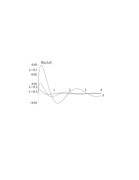
Figure 1: Behavior of $S(z,\lambda z)$ at different values of $\lambda$.

Let us rewrite expression (11) in the $d=2$ case in the dimensionless form

$$rj_{\varphi}(r)=\frac{1}{2\pi}\int\limits_{0}^{\infty}dz\,z\left[z^{2}+\left(\frac{mr_{0}}{\lambda}\right)^{2}\right]^{-1/2}S(z,\lambda z),$$ (30)

where $\lambda=r_{0}/r$ $(\lambda\in[0,1])$. In the limit of a singular filament ($r_{0}=0$) expression (30) can be reduced to the following form, see [20],

$$rj_{\varphi}^{sing}(r)=\frac{\sin(F\pi)}{\pi^{3}}\times\\ \times\int\limits_{mr}^{\infty}dw\frac{w^{2}}{\sqrt{w^{2}-(mr)^{2}}}\left\{w\left[K^{2}_{1-F}(w)-K^{2}_{F}(w)\right]+(2F-1)K_{F}(w)K_{1-F}(w)\right\}$$ (31)

($K_{\rho}(u)$ is the Macdonald function of order $\rho$) with asymptotics

$$rj_{\varphi}^{sing}(r)=e^{-1}rB^{sing}_{(I)}(r)=-\frac{\tan(F\pi)}{4\pi}\left(F-\frac{1}{2}\right)^{2}+O\left[(mr)^{2}\right],\,\,mr\ll 1$$ (32)

and

$$rj_{\varphi}^{sing}(r)=2me^{-1}r^{2}B^{sing}_{(I)}(r)=\frac{\sin(F\pi)}{2\pi}\left(\!F-\frac{1}{2}\right)\frac{e^{-2mr}}{\sqrt{\pi mr}}\left(1+O\left[(mr)^{-1}\right]\right),\,\,mr\gg 1,$$ (33)

where $B^{sing}_{(I)}(r)$ is the vacuum magnetic field which is induced in the $d=2$ case by a singular vortex filament. The total induced vacuum magnetic flux in this case, see (25), attains the maximal absolute value equal to $|e|/(72\sqrt{3}m)$ at $F=F_{\pm}$, where

$$F_{\pm}=\frac{1}{2}\left(1\pm\frac{1}{\sqrt{3}}\right).$$ (34)

Our primary task is to compute numerically the induced vacuum current in the $d=2$ case, see (30), at $F=F_{\pm}$, when the integral in (30) is likely to be most distinct from zero. It can be shown that $S(z,\lambda z)$ is an oscillating function with an amplitude that exponentially decreases at large $z$, see Fig.1. So, for a vortex tube of nonvanishing radius, we have to compute values of dimensionless quantity $rj_{\varphi}$ at different values of $\lambda$. To do this, we perform high-precision numerical integration in (30) with the help of a technique developed earlier in [16] – [19] for the computation of the vacuum energy density which is induced in the $d=2$ case by a vortex tube of nonvanishing radius.The results can be approximated by an interpolation function in the form

$$rj_{\varphi}(r)=\left[\frac{e^{-2x}}{\sqrt{x}}\right]\left[\left(\frac{x-x_{0}}{x}\right)^{2}\frac{P_{3}(x-x_{0})}{x^{3}}\right]\frac{Q_{3}(x^{2})}{R_{3}(x^{2})},\quad x>x_{0},$$ (35)

where $x=mr$, $x_{0}=mr_{0}$ and $P_{n}(y)$, $Q_{n}(y)$, $R_{n}(y)$ are polynomials in $y$ of the $n$-th order with the $x_{0}$-dependent coefficients. The first factor in the square brackets describes the large distance behavior in the case of a zero-radius tube (filament), the second factor in the square brackets is an asymptotics at small distances from the side surface of the tube, the last factor describes the behavior at intermediate distances. Since the vortex tube is impenetrable, $rj_{\varphi}(r)$ (35) vanishes at $x\leq x_{0}$.

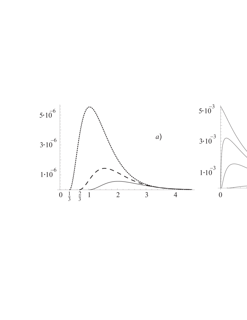
Figure 2: The dimensionless induced vacuum current ($rj_{\varphi}$) as a function of the dimensionless distance from the axis of the tube $(x)$ for different values of the dimensionless tube radius ($x_{0}$): (a) solid line corresponds to $rj_{\varphi}\cdot 10^{2}$ for $x_{0}=1$, dashed line corresponds to $rj_{\varphi}\cdot 10$ for $x_{0}=2/3$ and dotted line corresponds to $rj_{\varphi}$ for $x_{0}=1/3$; (b) the cases of a singular filament ($x_{0}=0$) and of a tube with $x_{0}=10^{-3},10^{-2},10^{-1}$ are from up to down on the plot. Variable $x$ is along the abscissa axis.

The results are presented on Fig.2. The current is negligible for the tube of large radius, i.e. of order of the Compton wavelength and larger, $r_{0}\geq m^{-1}$, see Fig.2a. But the current in the case of $r_{0}\ll m^{-1}$ is comparable with the current in the case of a singular filament; note that the former is always less in value than the latter, see Fig.2b.

Of particular interest is the behavior of the induced vacuum current as the tube radius decreases. However, a direct numerical computation in the case of $x_{0}<10^{-3}$ is a rather complicated task, needing a long computational time. To surmount these difficulties, one has to take account for the following two circumstances. On the one hand, the case of a singular filament is recovered as the tube radius tends to zero, $r_{0}\rightarrow 0$. On the other hand, in contrast to (32), the current in the case of the nonvanishing tube radius vanishes quadratically in the vicinity of the tube, see (35); this is in accordance with the analysis of the $r_{0}\rightarrow 0$ limit for the solution to the Klein-Fock-Gordon equation [21, 22]. Therefore it is reasonable to assume the following behavior at $r_{0}\ll m^{-1}$ and $r-r_{0}\ll m^{-1}$:

$$rj_{\varphi}(r)=\left(\frac{r-r_{0}}{r}\right)^{2}rj_{\varphi}^{sing}(r).$$ (36)

The expected asymptotic behavior of the current in the case of the extremely small tube radius ($r_{0}=10^{-9}m^{-1}$) is presented on Fig.3.

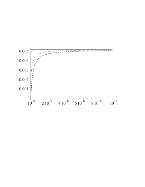
Figure 3: The expected behavior of the dimensionless induced current ($rj_{\varphi}$, dashed line) and the dimensionless induced magnetic field ($e^{-1}rB_{(I)}$, dotted line) at small distances from the side surface of the tube for the case of $x_{0}=10^{-9}$; solid line corresponds to the case of a singular filament ($x_{0}=0$), see (32). The variable $x$ $(x>x_{0})$ is along the abscissa axis.

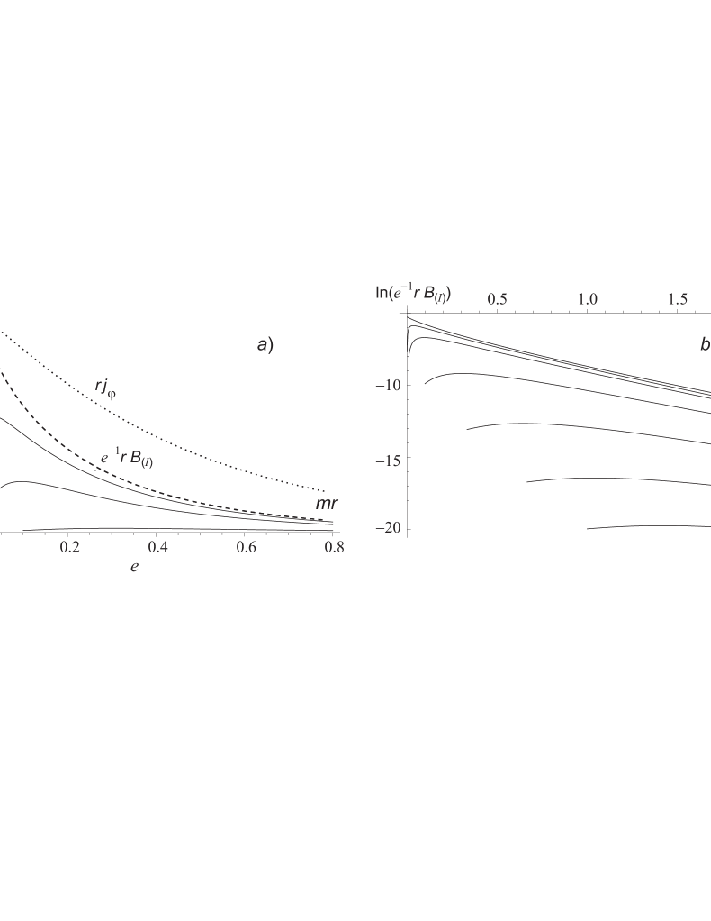
Figure 4: The dimensionless induced vacuum magnetic field $(e^{-1}rB_{(I)})$ outside of tubes of different radius: (a) the cases of a singular filament (dotted and dashed lines) and tubes with $x_{0}=10^{-3},10^{-2},10^{-1}$ are from up to down; (b) the case of a singular filament and tubes with $x_{0}=10^{-3},10^{-2},10^{-1},2/3,1/3,1$ in logarithmic scale are from up to down.

Using (18) and (35), we compute numerically $B_{(I)}(r)$, i.e. the induced vacuum magnetic field in the $d=2$ case. The results are presented on Fig.4 for the tube radius in the range $10^{-3}m^{-1}\leq r_{0}\leq m^{-1}$. As the tube radius decreases, the results approach to the result in the case of a singular filament, excepting the region in the vicinity of the tube. The expected asymptotic ($r\rightarrow r_{0}$) behavior of the induced vacuum magnetic field in the case of the extremely small tube radius ($r_{0}=10^{-9}m^{-1}$) is presented on Fig.3.

Using (21), (22), (30) and (35), we compute numerically the total induced vacuum magnetic flux in the $d=2,3,4$ cases, i.e. $\Phi_{2}^{(I)}$, $\Phi_{3}^{(I)}$ and $\Phi_{4}^{(I)}$. The results are presented on Fig.5 and in Table 1. In the $d=2$ case, the absolute value of the flux induced by a filament is always larger then the absolute value of the flux induced by a tube of the nonvanishing radius. As the spatial dimension increases, the induced flux becomes a more strongly decreasing function of the large tube radius ($r_{0}\gtrsim m^{-1}$) and a more strongly increasing function of the small tube radius ($r_{0}\ll m^{-1}$). Of particular interest is the realistic case of $d=3$. Whereas the induced flux in the unphysical case of a singular filament is infinite, see (27) and (29) in the limit $r_{0}\rightarrow 0$, the induced flux in the physical case of a tube of the nonvanishing radius is finite; for instance, it attains a noticeable value of $0.0065\,e$ at $r_{0}=0.001\,m^{-1}$ at $d=3$.

$x_{0}$	1	2/3	$1/3$	$10^{-1}$	$10^{-2}$	$10^{-3}$
${m\Phi^{(I)}_{2}}/e$	$2.355\cdot 10^{-8}$	$5.762\cdot 10^{-7}$	$2.071\cdot 10^{-5}$	$4.878\cdot 10^{-4}$	$3.657\cdot 10^{-3}$	$6.217\cdot 10^{-3}$
${\Phi^{(I)}_{3}}/{e}$	$3.07\cdot 10^{-9}$	$8.829\cdot 10^{-8}$	$4.129\cdot 10^{-6}$	$1.483\cdot 10^{-4}$	$2.223\cdot 10^{-3}$	$6.547\cdot 10^{-3}$
${\Phi^{(I)}_{4}}/{(me)}$	$2.06\cdot 10^{-10}$	$7.06\cdot 10^{-9}$	$4.43\cdot 10^{-7}$	$2.675\cdot 10^{-5}$	$1.254\cdot 10^{-3}$	$1.585\cdot 10^{-2}$

Tab.1 The dimensionless induced vacuum magnetic flux in cases of dimension $d=2,3,4$ for tubes of different radius.

4 Summary

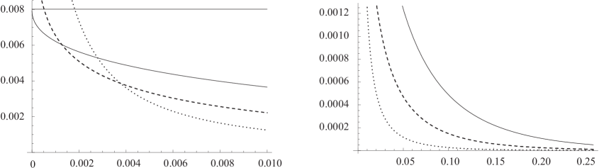
Figure 5: The dimensionless induced vacuum magnetic flux in spaces of different dimensionality as a function of the dimensionless tube radius $(x_{0})$: $e^{-1}m\Phi^{(I)}_{2}$ – solid line, $e^{-1}\Phi^{(I)}_{3}$ – dashed line, $(em)^{-1}\Phi^{(I)}_{4}$ – dotted line. The case of small $x_{0}$ is on the left, and the case of large $x_{0}$ is on the right. The case of $x_{0}=0$ and $d=2$ is presented by a horizontal solid line on the left.

In the present paper, we consider the current and the magnetic field which are induced in the vacuum of the quantized charged scalar matter field by a topological defect in the form of the ANO vortex. A perfectly reflecting (Dirichlet) boundary condition is imposed on the matter field at the side surface of the vortex. The induced current is circulating around the vortex, and the induced magnetic field is directed along the vortex. Both the current and the magnetic field are vanishingly small in the case of the vortex transverse size being of the order of or exceeding the Compton wavelength of the matter field (the dimensionless current is less than $10^{-8}$, the dimensionless total flux of the magnetic field is less then $10^{-9}$ in the $d=3$ case). Together with the results of [16, 19] about the Casimir force acting on the vortex side surface, this confirms the conclusion that the vacuum polarization of the quantized matter is almost absent in the case when the mass of the Higgs field (forming the topological defect) is of the order of or less than the mass of the matter field; the vacuum polarization effects are essential for matter fields with masses which are much smaller than a scale of the spontaneous symmetry breaking (Higgs mass). As to the induced vacuum current and magnetic field in the background of the ANO vortex, we show in the present paper that they are essential in this latter case, being odd in the value of the vortex flux, $\Phi$, and periodic in this value with with the period equal the London flux quantum, $2\pi{\tilde{e}}^{-1}$; to be more precise, they vanish at $F=0,1/2,1$, where $F$ is given by (13), and are of opposite signs in the intervals $0<F<1/2$ and $1/2<F<1$, with their absolute values being symmetric with respect to the point $F=1/2$. The current and the magnetic field decrease exponentially at large distances from the vortex, while otherwise they behave similarly to the case of a singular filament (vanishing transverse size) with the exception of a small vicinity of the vortex tube. The latter distinction allows us to eliminate an unphysical divergence which is present at $d\geq 3$ for the total induced vacuum magnetic flux in the case of a singular filament. As long as the nonvanishing transverse size of the vortex is taken into account, the total induced vacuum magnetic flux becomes finite, attaining quite realistic values for the case of the three-dimensional space even at the spontaneous symmetry breaking scale exceeding the mass of the matter field by just three orders of magnitude, see Fig.5 and Table 1. This can provide a possible mechanism for generating primordial magnetic fields by cosmic strings in early universe.

5 Acknowledgments

I.V.I. and Yu.A.S. acknowledge the support from the National Academy of Science of Ukraine (project No.0112U000054). The work of V.M.G. was supported by the Swiss National Science Foundation grant SCOPE IZ 7370-152581. The work of Yu.A.S. was supported by the ICTP-SEENET-MTP grant PRJ-09 ”Strings and Cosmology”.

References

• [1] A.A. Abrikosov, Sov. Phys.-JETP 5, 1174 (1957).
• [2] H.B. Nielsen and P. Olesen, Nucl. Phys. B 61, 45 (1973).
• [3] R.P. Huebener, Magnetic Flux Structure in Superconductors (Springer-Verlag, Berlin, 1979).
• [4] D.R. Nelson, Defects and Geometry in Condensed Matter Physics (Cambridge University Press, Cambridge, 1994).
• [5] G.E. Volovik, The Universe in a Helium Droped (Clarendon, Oxford, 2003).
• [6] A. Vilenkin and E.P.S. Shellard, Cosmic strings and other topological defects (Cambridge University Press, Cambridge UK, 1994).
• [7] M.B. Hindmarsh and T.W.B. Kibble, Rep. Prog. Phys. 58, 477 (1995).
• [8] E.J. Copeland and T.W.Kibble, Proc. Roy. Soc. A 466, 623 (2010).
• [9] V. Berezinsky, B. Hnatyk and A. Vilenkin, Phys. Rev. D 64, 043004 (2001).
• [10] R. Brandenberger, H. Firouzjahi, J. Karoubi and S. Khosravi, J. Cosmol. Astropart. Phys. JCAP01 (2009) 008.
• [11] M.G. Jackson and X. Siemens, J. High Energy Phys. JHEP06 (2009) 089.
• [12] Y. Aharonov and D. Bohm, Phys. Rev. 115, 485 (1959).
• [13] A. Tonomura, J.Phys. A: Math. Theor. 43, 35402 (2010).
• [14] Yu.A. Sitenko and N.D. Vlasii, Class. Quant. Grav. 26, 195009, (2009).
• [15] R. Jackiw, A.I. Milstein, S.-Y. Pi, and I.S. Terekhov, Phys. Rev. B 80, 033413 (2009).
• [16] V.M. Gorkavenko, Yu.A. Sitenko and O.B. Stepanov, J. Phys. A: Math. Theor. 43, 175401 (2010).
• [17] V.M. Gorkavenko, Yu.A. Sitenko and O.B. Stepanov, Int. J. Mod. Phys. A: 26, 3889 (2011).
• [18] V.M. Gorkavenko, Yu.A. Sitenko and O.B. Stepanov, Ukr. J. Phys. 58, No.5, 424 (2013).
• [19] V.M. Gorkavenko, Yu.A. Sitenko and O.B. Stepanov, Int. J. Mod. Phys. A 28, 1350161 (2013).
• [20] Yu.A. Sitenko and A.Yu. Babansky, Mod. Phys. Lett. A 13, 379 (1998); Phys. Atom. Nucl. 61, 1594 (1998).
• [21] V.G. Bagrov, D.M. Gitman and V.B. Tlyachev, J. Math. Phys. 42, 1933 (2001).
• [22] S.P. Gavrilov, D.M. Gitman, A.A. Smirnov and B.L. Voronov in: Focus on Mathematical Physics Research (Nova Science Publishers, New York, 2004), pp. 131-168.