Quark Masses from Lattice QCD

Abstract:

In this talk I review several topics concerning the determination of quark masses by means of lattice QCD simulations, with particular focus on recently introduced techniques of non-perturbative renormalisation, the determination of heavy quark masses, and the proper quantification of the source of isospin breaking effects in the light quark sector.

1 Introduction

Quark masses are fundamental parameters appearing in the QCD lagrangian, and as such they cannot be predicted by the theory. Instead, they are extracted from a comparison of theoretical expressions with experimentally measured values of various physical observables. Theories beyond the Standard Model, aiming at the grand unification of fundamental interactions and based on a specific gauge group, also predict the symmetry pattern amongst various Yukawa couplings which then translates into equalities amongst ratios of various fermion masses. The fundamental gauge group is then assumed to be acceptable as long as the theoretical ratios among quark/lepton masses agree with actual values. It is therefore of fundamental importance to reliably define and accurately determine the quark masses. On the practical side, quark masses decisively enter the theoretical expressions for a vast number of physical processes so that their more accurate values significantly improve the theoretical precision.

In that respect lattice QCD has played the essential role over the past two decades, and nowadays the values of the quark mass and $\alpha_{s}(\mu)$ are more and more dominated by the results from numerical simulations on the lattice. 

It is of crucial importance to properly define the quark mass. In pertutbation field theory the mass can be defined as a pole of the propagator. Such a definition, known as the pole quark mass, is a purely perturbative concept and suffers from infrared ambiguities known as renormalons. Non-perturbatively, however, the quark pole mass cannot be defined since the renormalised quark propagator has no distinct pole due to confinement in QCD.

The purpose of this review is to present an updated comparison of different determinations of the quark masses computed by means of numerical simulations of QCD on the lattice. As far as the light quark masses are concerned, most of the material has already been discussed in great detail in the FLAG review [1]. Here we only update those results and focus on a discussion of the mass difference $m_{d}-m_{u}$, for which results have been recently published. Most of this review is devoted to the lattice QCD determination of the heavy quark masses, a subject that has not been discussed in Ref. [1].

The values of bare parameters in the Lagrangian depend on the adopted regularisation. A meaningful comparison of various determinations of the quark mass values can be made only in a specific renormalisation scheme and at a specific renormalisation scale. It is customary to quote quark masses in the ${\overline{{\rm MS}}}$ scheme. The referential scale is $\mu=2$ GeV, which is expected to be large enough to make a parturbative matching between the ${\overline{{\rm MS}}}$ and a non-perturbative renormalization scheme (suitable for lattice studies) reliable, and to be small enough with respect to the hard lattice cut-off scale. With more and more simulations performed at very fine lattice spacings the referential scale is often pushed to $\mu=3$ GeV and will be pushed even higher. One should also stress that the choice of ${\overline{{\rm MS}}}$ as a reference renormalisation scheme is also made when comparing lattice results obtained by using different regularization schemes. That step is still widely adopted but is in principle unnecessary since the computation of the mass renormalization constant is made in renormalization schemes suitable for lattice QCD computations, such as RI-MOM [2], SF [3], RI-SMOM [4], but not ${\overline{{\rm MS}}}$, which is inherently perturbative.

In addition to the FLAG review released in 2013 [1], the Particle Data Group recently updated a section dedicated to the quark masses [5]. In that latter review the results obtained by using different approaches (sum rules, effective theories, lattices, etc.) have been combined and the quoted averages are shown to be heavily dominated by the results obtained from the studies of QCD on the lattice.

The remainder of the present review is organised as follows: In Sec. 2 we contextualise the determination of quark mass in the more general framework of renormalisation of QCD, describe a commonly used approach to determine quark masses and stress the importance of quark mass ratios; we will devote special attention to the additional problems arising when defining a mass indepentent renormalisation scheme in $n_{f}=2+1+1$ simulations, that are becoming more an more available. In Sec. 3 we discuss results obtained by using less common inputs to compute the quark masses on the lattice. In Sec. 4 we discuss an alternative method of computing the quark masses through the moments of correlation functions. Sec. 5 is devoted to various determinations of the $b$ quark mass, while in Sec. 6 we discuss the recent works in which the $d$-$u$ quark mass difference has been computed. We conclude in Sec. 7.

2 Renormalisation

The computation of quark masses starts by defining a procedure to tune bare parameters in such a way as to keep the physics unchanged while removing the cut-off. The lines of constant physics, described by such a set of parameters, are constrained to describe the real world in the continuum limit. A common procedure consists in reproducing the mass of the lightest pseudo-Goldstone bosons, and to use an additional quantity (such as the mass of $\Omega$, or a pion/kaon decay constant) to determine the lattice spacing. Light pseudoscalar meson masses are highly sensitive to the light quark masses, they are easy to compute on the lattice even with a limited numerical effort, and their dependence on quark masses is well described by the Chiral Perturbation Theory which can also be used to efficiently correct for the (exponentially small) finite volume effects of the lattice.

After tuning the quark masses to reproduce the physical pseudoscalar meson masses, the lattice regularised theory is renormalised, but to make sense of the bare parameters in the Lagrangian, further steps are needed. A renormalised quark mass can be introduced by means of the chiral vector Ward identity, which ensures that the product of the quark mass and the corresponding scalar density ($S=\bar{q}q$) is Renormalisation Group Invariant (RGI), and therefore $Z_{m}=1/Z_{S}$. In other words, in any renormalisation scheme that does not break the chiral symmetry,

$$m_{q}^{ren}(\mu)=Z_{m}(\mu)m_{q}^{bare}=m_{q}^{bare}/Z_{S}(\mu)\,.$$ (1)

Such relations allow for a meaningful notion of the renormalised quark mass at a fully non-perturbative level, in schemes such as RI-MOM, RI-SMOM or SF. Relations to the reference ${\overline{{\rm MS}}}$ renormalisation scheme can be established in perturbation theory. It is then a question which scale can be probed by the non-perturbative method, and then to assess whether or not that scale is high enough to keep the uncertainties due to truncation in perturbative expansion small.

For example, the Rome-Southampton Method (RI-(S)MOM) to compute the renormalisation constants non-perturbatively requires the existence of a window $1/L\ll\Lambda_{QCD}\ll\mu\ll\pi/a$, with $L$ being the length of a side of the lattice box, in which the uncertainties related to the finite cut-off and to the perturbative matching to other renormalisation schemes are controllable and small. In practice this requirement translates to the condition that the lattice spacings should be smaller than about 0.1 fm ($a^{-1}\simeq 2$ GeV). In the case of staggered quark action, however, additional complications prevented so far a simple implementation of the procedure.

The scaling window needed in the RI-(S)MOM is not needed in the method based on the use of SF where a series of additional simulations need to be made with special boundary conditions on a box of finite extension $T$, which ensure the renormalisation scale to be $\mu=1/T$.

When non-perturbative renormalisation methods cannot be easily applied, one can rely on the QCD perturbation theory to compute $Z_{m}(\mu)$. Unfortunately, however, perturbative calculations on the lattice become rapidly too complex with an increase in the order of the perturbative expansion, which in practice means that going beyond two loops becomes extremely difficult to do (cf. the three loop stochastic computation presented by M.Brambilla at this conference [6]).

In Sec. 4 we will discuss a sophisticated approach that allows to make use of high-order continuum perturbation theory. Before discussing in detail the renormalisation of $n_{f}=2+1+1$ simulations, we comment extensively on the physical content of ratios of bare quark masses.

2.1 RGI ratios of quark masses

The knowledge of $am^{bare}(a)$ is already of invaluable importance. If the regularisation preserves the chiral symmetry (or its $U(1)_{A}$ remnant), the quark masses renormalises multiplicatively, so that in the mass independent renormalisation schemes ($\partial Z_{m}/\partial m_{q}=0$) the ratio of renormalised quark masses is equal to the ratio of bare quark masses:

$$\frac{m_{q_{1}}^{ren}}{m_{q_{2}}^{ren}}=\frac{am_{q_{1}}^{bare}}{am_{q_{2}}^{bare}}\,.$$ (2)

This relation holds as long as QED is not included in the simulation. The above conditions are respected (for example) in the computations made by the Fermibalb/MILC collaboration [7] (cf. also contribution by J. Komijani at this conference) based on their recent $n_{f}=2+1+1$ HISQ regularised quark simulations. To determine the ratio between the strange quark mass $m_{s}$ and the average of up and down quark masses, $m_{l}=(m_{u}+m_{d})/2$, they proceeded in two steps. First, at each value of the lattice spacing they tuned the bare light quark masses in such a way that $\frac{\left(a^{2}\right)M_{\pi}^{2}\left(am\right)}{\left(a^{2}\right)f_{\pi}^{2}\left(am\right)}$ computed on the lattice reproduces the experimentally measured $\left(M_{\pi}/f_{\pi}\right)_{exp}^{2}$. The resulting $am_{l}^{bare}$ is then converted to physical units after using the lattice spacing $a$ extracted from $af_{\pi}\left(am_{light}^{bare}\right)=f_{\pi}^{exp}$. The bare strange quark mass, instead, is fixed by tuning $M_{ss}^{2}=2M_{K}^{2}-M_{\pi}^{2}$ to its physical value (see left panel of Fig. 1). To LO in ChPT $M_{ss}^{2}$, is independent on $m_{l}$, so the tuning of $m_{s}$ almost decouples from that of $m_{l}$. With such a determined value of $m_{s}$, the charm quark mass $m_{c}$ is obtained from the requirement that the mass of the heavy-strange pseudoscalar meson coincides with $M_{D_{s}}^{exp}$.

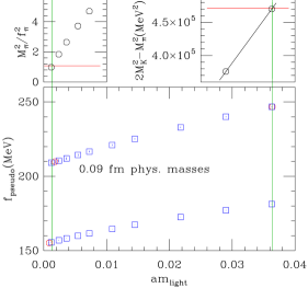
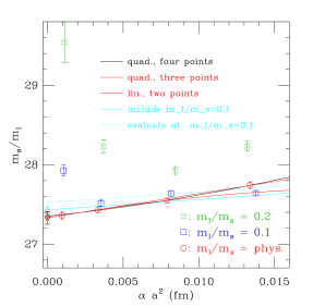
Figure 1: Left panel: tuning of the light and strange quark masses at a fixed lattice spacing (0.09 fm); different points corresponds to mesons simulated numerically, with quarks of common mass $m_{l}$ (x-axis), where vertical green lines show the value of $m_{l}$ at which the interpolation of $M^{2}_{\pi}/f^{2}_{\pi}$ (top-left inset), $2M^{2}_{K}-M^{2}_{\pi}$ (top-right) and the decay constant $f$ (bottom) reproduce their physical value (red horizontal lines). Right panel: continuum extrapolation of the ratio computed at various lattice spacings. Plots taken from Ref. [7].

The ratios $m_{s}/m_{l}$ and $m_{c}/m_{s}$ are computed at each lattice spacing, and are then extrapolated to the continuum limit as shown in the right panel of Fig. 1 resulting in

$$m_{s}/m_{l} = 27.35(5)(^{+10}_{-7})\,,$$ (3)

$$m_{c}/m_{s} = 11.747(19)(^{+59}_{-43})\,.$$ (4)

These are the most accurate results for the quark mass ratios to date.

2.2 Renormalisation constants in $\boldsymbol{n_{f}=2+1+1}$ simulations

The ETM collaboration was the first to produce results for quark masses from simulations including $N_{f}=2+1+1$ dynamical quark flavours. Results presented in Ref. [8] were obtained from the analysis along the lines of their previous work with $N_{f}=2$ [9]. They computed non-perturbatively the mass renormalisation constants in the RI-MOM renormalisation scheme and performed matching to the ${\overline{{\rm MS}}}$ renormalisation scheme by using the expressions derived to four loops in perturbation theory [10]. In order to define a mass-independent renormalisation scheme, the renormalisation scale $\mu$ must be much larger than all the other scales of the theory, and, in particular, we must have $\mu\gg m$, with $m$ the mass of the heaviest quark. In RI-MOM scheme this is achieved by defining renormalisation constants at the chiral point.

In the case of their previous $n_{f}=2$ set of simulations, ETM collaboration computed renormalisation constants on the same set of gauge configurations used to measure hadronic observables. Extrapolating to the chiral limit in that case comes as a virtue out of the necessity to simulate a wide range of non-physical sea pion masses (280-500 MeV) needed for controlled extrapolation of observables to the physical point at which the sea pion mass is $m_{\pi}^{phys}$.

Conversely, results obtained from simulations carried out around the physical charm quark mass in the new $n_{f}=2+1+1$ simulations cannot be safely extrapolated to the chiral limit of the four quark masses. Therefore the renormalisation constants cannot be computed directly on $n_{f}=2+1+1$ configurations on which bare quark masses are computed.  To overcome this problem, the ETM collaboration specifically generated a set of gauge configurations with $n_{f}=4$ mass degenerate light quarks. The mass of the dynamical quarks is varied as to allow a continuum extrapolation [11] of the renormalisation constants. With these ingredients at hand the average up-down, strange and the charm quark masses were found to be:

$$m_{l}^{\overline{{\rm MS}}}(2\,{\rm GeV}) = 3.70(17)\,{\rm MeV}\,,$$ (5)

$$m_{s}^{\overline{{\rm MS}}}(2\,{\rm GeV}) = 99.6(4.3)\,{\rm MeV}\,,$$ (6)

$$m_{c}^{\overline{{\rm MS}}}(m_{c}) = 1.348(46)\,{\rm GeV}\,.$$ (7)

The authors also noted the advantage of working with ratios of similar quantities (eg. $M_{\pi}/M_{\bar{s}s}$, $M_{D_{s}}/M_{\bar{c}^{\prime}s}$), because they are less sensitive to cut-off effects and therefore their continuum extrapolation is much smoother.

Another possibility to define a mass independent scheme is to use the Schrödinger Functional (SF) renormalisation procedure, where simulations can be carried out directly in the massless theory, thus avoiding the need to extrapolate to the chiral limit. In the theory in which the heavy quarks $m_{h}$ are included, one can use the Step Scaling approach to evolve the renormalisation constants computed with physical (massive) heavy quarks up to a scale $\mu\gg m_{h}$, so that the terms $\propto(m_{h}/\mu)^{n}$ can be safely neglected. Such an approach is currently being investigated by the RBC/UKQCD collaboration (cf. J. Frison contribution, Ref. [12]).

3 Other physical inputs

3.1 Fixing the quark masses through the baryon spectrum

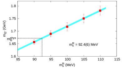
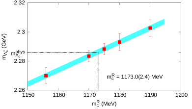
Figure 2: Interpolation of $\Omega^{-}$ (left panel) and $\Lambda_{c}^{+}$ (right panel) baryons respectively to physical renormalised strange and charm quark mass. Plots taken from Ref. [13].

Of all the possible observables used to compare theory and experiments to extract the values of physical quark masses, the most commonly used are the pseudoscalar meson masses, mainly because they are the simplest physical quantities to compute on the lattice and the corresponding results are very accurate. Nonetheless it is possible to use other quantities. For example, the ETM collaboration has recently reported on their results for the strange and charm quark masses by computing the baryon masses on the same set of $n_{f}=2+1+1$ gauge configurations already discussed above, in Sec. 2.2 (see also the contribution by Ch.Kallidonis at this conference [13]).

More specifically, they fixed $m_{s}$ from $\Omega$, the valence configuration of which is $sss$, and $m_{c}$ from the singly charmed baryon $\Lambda_{c}$. By linearly interpolating the baryon masses expressed in terms of $m_{s}^{ren}$ and $m_{c}^{ren}$ to their physical values, as illustrated in Fig. 2, they were able to extract the quark masses, while the lattice spacing has been determined by using the pion and/or the proton mass. The continuum and chiral extrapolations are made by relying on an empirical ansatz,

$$M_{\Omega} = M_{\Omega}^{chir}+c_{\Omega}M_{\pi}^{2}+d_{\Omega}a^{2}\,,$$ (8)

$$M_{\Lambda_{c}} = M_{\Lambda_{c}}^{chir}+c_{\Omega}^{\left(2\right)}M_{\pi}^{2}+c_{\Omega}^{\left(3\right)}M_{\pi}^{3}+d_{\Omega}a^{2}\,.$$ (9)

Lacking a solid effective theory framework to perform chiral extrapolation and to reliably estimate the finite volume effects, this analysis is more challenging than those based on using the pseudoscalar mesons, mainly because of the difficulties in assessing the size of systematic errors. The resulting strange and charm quark masses,

$$m_{s}^{\overline{{\rm MS}}}(2\,{\rm GeV}) = 92.4(0.6)(2.0)\,{\rm MeV}$$ (10)

$$m_{c}^{\overline{{\rm MS}}}(2\,{\rm GeV}) = 1.173(2)(17)\,{\rm GeV}\,,$$ (11)

appear to be in reasonable agreement with values obtained when using mesons as inputs, Eqs. (6, 7), which is an encouraging consistency check. We reiterate that the systematic error estimates in Eqs. (10, 11) are presumably less robust than those presented in Eqs. (6, 7).

3.2 Global fit approach

It is a common practice to determine the quark masses in dedicated lattice QCD analysis, by choosing a minimal number of inputs to renormalise the theory, and then to use the obtained quark mass values in calculations of other physical quantities.

Recently the RBC/UKQCD collaboration has presented a large set of results obtained from simulations performed around the physical pion mass [14]. In order to correct for the (small) difference between the simulated quark mass and the physical one they made a very short $\mathcal{O}(3\%)$ chiral extrapolation in which they combined the results of simulations made near the physical pion mass with those corresponding to heavier pions. In addition to the three experimental inputs used to tune the physical light quark masses ($m_{\pi}$, $m_{K}$ and $M_{\Omega}$), they computed several other quantities ($f_{\pi}$, $f_{K}$, $B_{K}$, …) and then performed a simultaneous fit of all the data by using the expressions derived in chiral perturbation theory in which they were able to further monitor the dependence of each physical quantity on the sea quark mass. Such a dependence further constrains the quark masses, the values of which turn out to be extremely accurate, namely,

$$m_{l}^{\overline{{\rm MS}}}(3\,{\rm GeV}) = 2.997(49)\,{\rm MeV}$$ (12)

$$m_{s}^{\overline{{\rm MS}}}(3\,{\rm GeV}) = 81.64(1.17)\,{\rm MeV}\,.$$ (13)

We notice that a global fit approach allows to determine all the observables while keeping all correlations under control. The approach could be in principle extended to include even more observables, but it becomes more complicated to verify consistency of different fit ansätze.

4 Renormalised quark mass from the moments of correlation functions

A few years ago the HPQCD group has proposed to bypass the intermediate step non-perturbative renormalisation and obtain directly the renormalised quark mass in the ${\overline{{\rm MS}}}$ scheme, by computing an RGI quantity on the lattice and matching it to its counterpart computed in the continuum perturbation theory, expressed in terms of the ${\overline{{\rm MS}}}$ quark masses and the running coupling [15].

Moments of the correlation function are nowadays used in lattice QCD for a range of different quantities. In Ref. [15] they have been used for the first time to compute the charm quark mass.

After summing up the correlation function over the space, one first defines the moments with respect to time,

$$G_{n}^{\left(j\right)}=\sum_{t}{\left(t/a\right)^{n}}G^{\left(j\right)}\left(t\right),\qquad G^{\left(j\right)}\left(t\right)=\left(am_{c}^{bare}\right)^{2}\sum_{\vec{x}}\left\langle j\left(\vec{x},t\right)j(\vec{0},0)\right\rangle\,,$$ (14)

where $G_{n}^{\left(j\right)}$ is the $n$-th moment of the non-perturbatively computed two-point correlation function, $j=\bar{c}\Gamma c$ ($\Gamma=\gamma_{5},\gamma_{\mu}$), with all quantities being unrenormalised. One then forms the convenient double ratios of moments $G_{n}^{(j)}$ and their values $G_{n}^{(j0)}$ computed to LO in lattice perturbation theory,

$$R_{n}^{\left(j\right)}=\frac{M_{mes\,j}}{2m_{c}^{0}}\sqrt{\frac{G_{n}^{\left(j\right)}}{G_{n-2}^{\left(j\right)}}\frac{G_{n-2}^{\left(j0\right)}}{G_{n}^{\left(j0\right)}}}\,,$$ (15)

the quantities known as reduced moments. In the above expression $M_{mes}$ is the meson mass, and $m_{c}^{0}$ is the bare mass of the charm pole mass computed in lattice perturbation theory. Such a mixture of perturbative and non-perturbative quantities benefits from the following advantages:

• renormalisation constant of the operator $j$ cancel in the ratio, and $R_{n}$ is an RGI quantity;

• cut-off effects, finite volume effects and the statistical noise largely cancel in the ratio;

• the introduction of a leading order calculation of the moments additionally suppresses cut-off effects, so that the ratios $R_{n}$ can be smoothly extrapolated to the continuum limit.

As a last comment, we notice that the expressions for $R_{n}$ become simpler if the currents used in the correlation function satisfy a Ward Identity, because it is possible to form the RGI quantities more easily.

Most importantly, as an effect of the known exponential decay in space-time, moments of correlation function are largly dominated by the short distance physics contribution, which means that for values of $n$ not too large ($n\lesssim 10$), $R_{n}$ is expected to be reliably reproduced by perturbation theory. One can deduce the values of the quark mass $m_{c}^{\overline{{\rm MS}}}(\mu)$ and of the running coupling $\alpha_{s}^{\overline{{\rm MS}}}(\mu)$ by comparing this result with the continuum perturbation theory prediction,

$$R_{n}^{PQCD}=\frac{r_{n}^{PQCD}\left(\alpha_{\overline{{\rm MS}}},\mu/m_{c}\right)}{2m_{c}^{\overline{{\rm MS}}}\left(\mu\right)/M_{mes\,j}}\,,$$ (16)

where $r_{n}^{PQCD}$ has been derived at three loop [16].

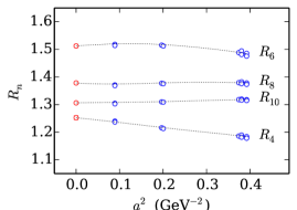
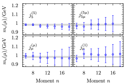
Figure 3: Left panel: continuum extrapolation of ratios of different order (plot taken from Ref. [17]). Right panel: $mc(\mu)$, for $\mu$ = 3 GeV and $n_{f}$ = 4 flavors, from moments of correlators built from four different lattice operators (grey band marking the final results).

In the left panel of Fig. 3 we show the extrapolation to the continuum limit of the reduced moments $R_{4,6,8,10}$ computed numerically by the HPQCD collaboration, after tuning the bare quark mass $am_{c}^{bare}$ in such a way as to reproduce $M_{\eta_{c}}$. In the right panel is shown the result of $m_{c}(\mu)$ obtained from comparison of the lattice results with the expression (16), for several types of currents and for a wide range of moments.

The approach proposed by HPQCD collaboration is inspired by the quark-hadron duality sum rules in which the moments of correlation function are estimated non-perturbatively by connecting the experimental data for differential electron-positron annihilation cross section, $d\sigma(e^{+}e^{-}\to\gamma^{\ast}\to X)/ds$, with perturbative QCD computations, in order to extract the heavy quark mass and the running coupling. In the method proposed here, instead of using the experimental data one computes the moments directly on the lattice and by using various Dirac structures.

HPQCD collaboration performed various tests to check the stability of $m_{c}\left(\mu\right)$ with respect to the variation of $n$, and the compatibility of the results obtained from different correlation functions. The analytic parametrisation of Eq. (16) of $R_{n}$ has also been extended by including the leading power correction, proportional to the gluon condensate, in order to try and quantify the non-pertubative effects. Those effects are, however, found to be negligible. 

In their recent paper [17] the HPQCD collaboration reported on their calculation of the charm quark mass obtained on the set of $n_{f}=2+1+1$ gauge field configurations produced by the MILC collaboration in which the improved (HISQ) regularisation of the sea quarks has been implemented. In other words, in their calculation the effects of the charm quark on the polarization of the QCD vacuum have been taken into account, while the light quark mass is varied down to the physical pion mass. By introducing a simplified version of the ratios, and after setting the scale by using $w_{0}$ instead of $r_{1}$, they obtained, $m_{c}(3\,{\rm GeV},{n_{f}}=4)=0.9851(63)\,{\rm GeV}$, in good agreement with their previous result (cf. Ref. [18]) $m_{c}(3\,{\rm GeV},{n_{f}}=3)=0.986(6)\,{\rm GeV}$ . Combining the renormalised value of the charm quark mass with the updated determination of the charm/strange quark mass ratio, $m_{c}/m_{s}=11.652(65)$, they also provided an accurate estimate of the strange quark mass, $m_{s}(2\,{\rm GeV},n_{f}=3)=93.6(8)\,{\rm MeV}$ and of the $b$ quark mass, $m_{b}^{\overline{{\rm MS}}}(m_{b},\,n_{f}=5)=4.162(48)\,{\rm GeV}$. This whole approach can be interpreted as a way to compute the quark mass renormalisation constant, $Z_{m}^{\overline{{\rm MS}}}(1/a)=m_{c}^{\overline{{\rm MS}}}(1/a)/am_{c}^{bare}/a$, by using $M_{mes\,j}$ as a physical input.

Results presented by the HPQCD collaboration are very accurate, and a natural question arises: are the moments of correlation functions a viable tool to increase the accuracy of lattice QCD determinations? So far, only the ETM collaboration implemented the method of moments in the computation by using the gauge field configurations with $n_{f}=2$ dynamical light quarks [19]. Their preliminary results, $m_{c}(3\,{\rm GeV},n_{f}=3)=\{0.979(9),\,0.998(14)\}\,{\rm GeV}$, based on two different chiral extrapolation procedures, are in good agreement with the values reported by the HPQCD collaboration, as well as with the previous result of ETMC obtained by using the standard method on the same set of gauge field configurations and by implementing the non-perturbative RI-MOM renormalisation program [9]. Given the lack of a comprehensive study of systematic errors, it remains difficult to estimate the improvement induced by the use of ratios of moments of correlation functions instead of the ordinary non-perturbative renormalisation, nor is it possible to accurately verify the compatibility of the results and assess the ultimate question concerning the overall control of non-perturbative effects of the method. One can only be comforted by the circumstantial evidence of the smallness of the gluon condensate contribution detected in [17], suggesting that the ambiguity in separation of the perturbative and non-perturbative effects affects the results well below the current precision.

In conclusion, moments of correlation functions have not yet been shown to be clearly superior to ordinary methods to define renormalised quark mass, but are certainly a key factor to allow a precise determination in those lattice frameworks where setting up a non-perturbative renormalisation program is notoriously difficult (for example in the staggered regularisation).

5 $b$ quark mass

Typical lattice spacings used in current lattice QCD simulations are larger than (or of the same order as) the scale involved in the physics of $b$ quark. For example $M_{B^{+}}=5.279\,{\rm GeV}$ while a typical range of (inverse) lattice spacings of the lattice simulations is $[2\div 4]$ GeV. For this reason specific methods dedicated to treatment of the $b$-quark on the lattice have been designed. In the following we describe modern approaches used to determine the $b$ quark mass.

5.1 Binding energy of non-relativistic heavy meson

Non-Relativistic QCD (NRQCD) [20] is an effective expansion of the QCD Lagrangian in terms of quark velocity $v$. The framework is used to describe a series of physical quantities, ranging from hadron spectroscopy to the hadronisation effects in decay amplitudes. In Ref. [21] it was proposed for the first time to compute the quark mass in NRQCD through an analysis of the binding energy in the bottomium system, namely,

$$M_{\Upsilon}^{exp}=2m_{b}^{pole}+\Delta M_{\Upsilon}\,,$$ (17)

where $m_{b}^{pole}$ is the pole mass of $b$ quark and $\Delta M_{\Upsilon}$ is the binding energy. Although the separation between the two contributions is plagued by the renormalon ambiguity, that ambiguity cancels out when converting the pole mass to the quark mass renormalised in the ${\overline{{\rm MS}}}$ scheme. Therefore an accurate computation of the binding energy could be in principle used to obtain $m_{b}^{\overline{{\rm MS}}}(\mu)$.

One first fixes the bare quark mass in the NRQCD Lagrangian, by matching the spin averaged bottomium mass computed on the lattice with the corresponding experimental value 

$$\overline{M_{b\bar{b}}}=a^{-1}\left(3aM_{\Upsilon}+aM_{\eta_{b}}\right)/4\,.$$ (18)

In NRQCD the zero of the energy is shifted so that the dispersion relation for a meson reads:

$$E(\vec{p})=E(0)+\sqrt{M+\vec{p}^{2}}-M\,,$$ (19)

where the rest energy $E(0)$ differs from the meson mass $M$ by an unknown constant and thus cannot be used to directly fix the bare quark mass. Instead, the simulated value of $M$ can be extracted by studying the dispersion relation of mesons, as shown in Eq. (19). The binding energy can be computed through the relation,

$$\Delta M_{\Upsilon}=E_{\Upsilon}(0)-2E_{0}\,,$$ (20)

where $E_{0}$ is the energy of an isolated $b$ quark, determined perturbatively.

With these ingredients in hands, the pole quark mass can be computed as

$$m_{b}^{pole}=M_{\Upsilon}^{exp}-\left[E_{\Upsilon}(0)-2E_{0}\right]\,,$$ (21)

which is then matched to the ${\overline{{\rm MS}}}$ scheme by using the continuum perturbation theory at the same order used to define the binding energy.

NRQCD is a non-renormalisable effective theory. The subtraction defined in Eq. (20) involves quantities that diverge as $a^{-1}$ in the continuum limit. Power divergence cannot be completely and unambiguously eliminated by means of perturbation theory, so that even after subtracting $E_{0}$ the binding energy contains a not-fully cancelled divergent term. This implies that no continuum limit of the right-hand side of Eq. (21) can be defined, and indeed previous steps did not include it. In lattice NRQCD one is confined to work in a range of lattice spacings small enough to keep the cut-off effects are under control, but large enough to avoid the sizable $\mathcal{O}(a^{-1})$ effects. Instead of a real continuum limit, only a comparison of results obtained at different lattice spacings can be made, and the difference amongst different ensembles is included in the budget of systematic uncertainties.

In their recent work the HPQCD collaboration presented results based on two different lattice spacings of the $n_{f}=2+1$ ASQtad gauge configurations produced by the MILC collaboration and the NRQCD action [22]. The subtraction in Eq. (20) is carried out to two loops using a mixture of automatised perturbation theory (cfr. C.Monahan at lattice conference 2013 [23]) and simulations performed at high $\beta$. Their final result,

$$m_{b}^{\overline{{\rm MS}}}\left(m_{b},\,n_{f}=5\right)=4.166(43){\rm GeV}\,,$$ (22)

is a very significant improvement of their first calculation presented in Ref. [21], in which the subtraction of the divergence had been carried out only to one loop.

Nonetheless it must be stressed that the ambiguity in cancellation of the power divergence is an intrinsic feature of NRQCD that limits the precision of the approach. When the method was proposed in Ref. [21], it allowed to carry out the first unquenched computation of the $b$ quark mass. Today, more reliable approaches exist and the NRQCD results can be viewed as a consistency check of other lattice methods.

5.2 Matching HQET and QCD

Heavy Quark Effective Theory (HQET) is another effective theory of QCD based on heavy quark symmetry which provides an expansion in the inverse heavy quark mass $1/m_{h}$. Contrary to NRQCD, HQET can be matched to QCD order by order in $1/m_{h}$ without running into troubles related to the subtraction of the power divergent term. After a long effort, the Alpha collaboration performed a fully non perturbative matching of HQET to QCD at $\mathcal{O}\left(1/m_{h}\right)$ [24],

$$\mathcal{L}^{HQET}=\bar{\psi}_{h}\left[\left(D_{0}+m^{bare}\right)-\omega_{kin}\mathbf{D}^{2}-\omega_{spin}\boldsymbol{\sigma}\cdot\mathbf{B}\right]\psi_{h}\,,$$ (23)

where the parametres $\omega_{kin}$ and $\omega_{spin}$ were computed by applying the step-scaling method on the gauge field configurations that include $n_{f}=2$ Wilson improved dynamical light quarks, and by using SF technique. To that order in heavy quark expansion one can write,

$$M_{B} = m^{bare}_{b}+E_{stat}+\omega_{kin}E_{kin}+\omega_{spin}E_{spin}\,,$$ (24)

where $E_{stat}$ is determined from the correlation function of the static heavy-light pseudoscalar/vector meson, while $E_{kin}$, $E_{spin}$ are determined from time behaviour of the correlation functions which include operator insertions of $\mathbf{D}^{2}$ and $\boldsymbol{\sigma}\cdot\mathbf{B}$, respectively.

To determine $m_{b}^{bare}$, one interpolates $M_{B}\left(m_{b}^{bare}\right)$ to reproduce $M_{B}^{exp}$, while simultaneously extrapolating to the physical pion mass and to the continuum limit. They determined $m_{b}^{RGI}$ by studying the running of the quark mass in the SF renormalization scheme and finally converted it to $m_{b}^{\overline{{\rm MS}}}(m_{b})$ using the continuum perturbation theory. Their result for the $b$ quark mass,

$$m_{b}^{\overline{{\rm MS}}}(m_{b},\,n_{f}=5)=4.21(11)\,{\rm GeV}\,,$$ (25)

was presented in Ref. [25], which improved their previous result based on quenched simulations [26]. More importantly, $1/m_{h}$ corrections included in the new study turned out to be very small, showing a reassuring convergence of HQET at the scale of the $b$ quark mass, and thus warranting the robustness of the approach.

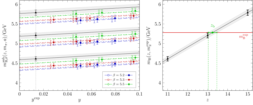
Figure 4: Chiral and continuum limit extrapolation (left panel) and interpolation to $b$ quark mass $z\propto m_{b}^{RGI}$ (right panel) of $M_{B}$ in HQET. Plots taken from Ref. [25].

5.3 Ratio method

Finally, we discuss the method adopted by ETMC, in which the observables used to fix the $b$ quark mass are computed at the scale of the $b$ quark by interpolating between the results obtained around the heavy charm quark mass and the static quark mass limit. To be able to do so they adopted the so-called ratio method [27], inspired by the Step-Scaling approach proposed in Ref. [28]. This method benefits from the heavy quark symmetry relation,

$$\lim_{m_{h}\to\infty}\frac{M_{hl}}{m_{h}}=1\,,$$ (26)

by considering a geometric series of masses $m^{\left(0\right)}=m_{c}$, $m^{\left(1\right)}=\lambda m_{c}$, … , $m^{\left(n\right)}=\lambda^{n}m_{c}\,$, from which one computes ratios of $M_{hl}$ between two consecutive values of the heavy quark mass,

$$y\left(m_{h}^{\left(n\right)},\,\lambda;\,m_{l},\,a\right)=\lambda\frac{M_{hl}\left(m_{h}^{\left(n\right)};\,m_{l},\,a\right)}{M_{hl}\left(m_{h}^{\left(n\right)}/\lambda;\,m_{l},\,a\right)}\,.$$ (27)

Important advantages in computing these ratios on the lattice are a large cancellation of cut-off effects, and a strong reduction of statistical noise. Each ratio is extrapolated to the continuum limit and to the physical Pion mass. The value of $M_{hl}(\lambda^{n}m_{c})$ can be reconstructed by fitting the first $y^{1}\dots y^{k}$ ratios as a function of $m_{h}=\lambda^{k}m_{c}$ up to values $k<n$ where the cut-off effects are under control, and one can then easily compute $M_{hl}(\lambda^{n}m_{c})=M_{cl}y(\lambda m_{c})y(\lambda^{2}m_{c})\dots y(\lambda^{n}m_{c})$ using the $y$ values from the fit ansatz. In this fit a heavy quark symmetry relation, Eq. (26), constrains the fit function and transforms the extrapolation to interpolation.

With a given parameter $\lambda$, and in order to reproduce the physical value $M_{B}$, one needs $j$ ratios, so that the quark mass $m_{b}$ can be finally determined by reconstructing the corresponding value $m_{b}=\lambda^{j}m_{c}$. In Ref. [29] the ETM collaboration provided a preliminary result for $b$ quark mass,

$$m_{b}^{\overline{{\rm MS}}}(m_{b})=4.26(16)\,{\rm GeV},$$ (28)

from simulations with $n_{f}=2+1+1$ twisted mass quarks, thus improving their previous result [30].

It must be stressed that the method relies substantially on the cancellation of cut-off effects when computing ratio of an observable at two close masses. This cancellation can and must be checked on a case by case approach. In particular it has been shown to happen in Twisted Mass, for a set of observables. In other regularisations or for other observables the cut-off effects might change in a less controlled way with the heavy quark mass, in which case the reduction of cut-off effects would be only mild and the ratio method itself of limited utility.

6 $d$-$u$ quark mass difference

Isospin is a good symmetry of the strong interaction. Smallness of the isospin breaking effects warrants reliability of the calculations performed in the isospin symmetric limit of lattice QCD, in which it is assumed that $m_{u}=m_{d}=m_{l}$, and charge are electrically neutral ($e=0$). On the other hand that same smallness makes difficult to determine the mass difference $\delta m_{ud}=(m_{d}-m_{u})/2$ itself. Far from being a matter of purely conceptual relevance, determining separately the mass of the light quarks answers deep theoretical questions: for instance if the $u$ quark was massless, the CP-violating term $\theta_{QCD}F\tilde{F}$ would not impact any physical observable, which would then explain why the measured value of $\theta_{QCD}$ is apparently so small (strong CP puzzle).

An updated review of the inclusion of QED into lattice QCD simulations has been presented at this conference by A. Portelli. In the following we will cover only the aspects strictly related to the quark masses. Including QED in the QCD Lagrangian complicates the pattern of renormalisation of quark masses. Quarks of different charges receive QED corrections that evolve in different ways under the renormalisation group. For this reason, ratios of quark masses of different charges are no longer RGI quantities (though the effect induced by different running is largely negligible at the level of current precision). Similarly the separation of the contribution of QCD and QED to physical observables is a matter of convention, because their sources (quark mass difference, QED corrections) get mixed up under renormalisation. The exact separation of QCD and QED effects requires an additional renormalisation condition, though a broad range of sensible schemes can be considered to be equivalent at the level of current precision.

Thanks to isospin and charge symmetries, the mass of neutral pion receives corrections due to the breaking of isospin only at (highly suppressed) $\mathcal{O}\left(e^{2}\delta m_{ud}\right)$. This makes its experimental value $M_{\pi}^{0}=135\,{\rm MeV}$ appropriate to determine the average mass of the light quarks $m_{l}$. The difference between the neutral and charged Pion masses at leading order in the isospin breaking is an $\mathcal{O}(e^{2})$ effect, whereas the contribution due to $\delta m_{ud}$ starts from $\mathcal{O}(\delta m_{ud}^{2})$, and thus cannot be efficiently used to determine $m_{u}$ and $m_{d}$ separately. The easiest solution is to consider to the difference of masses of $K$ mesons. Such a strategy has been followed by three different groups.

The RM123 collaboration included in a non-perturbative QCD framework the leading order isospin breaking terms on the $n_{f}=2$ gauge configurations generated by ETMC, and obtained [31]

$$m_{u,\,d}^{\overline{{\rm MS}}}(2\,{\rm GeV}) = \left\{2.40(15)(17),\,4.80(15)(17)\right\}\,{\rm MeV}\,,$$ (29)

$$m_{u}/m_{d} = 0.50(2)(3)\,.$$ (30)

The BMW collaboration combined the determination of the ChPT Low Energy Constant $B_{2}$ [32] with the Kaon meson mass difference of [33], to obtain the preliminary results

$$m_{u,\,d}^{\overline{{\rm MS}}}(2\,{\rm GeV}) = \left\{2.29(6)(5),\,4.65(6)(5)\right\}\,{\rm MeV}\,,$$ (31)

$$m_{u}/m_{d} = 0.49(1)(1)\,.$$ (32)

Finally, the MILC collaboration presented their preliminary results for $m_{u}/m_{d}$ based on the update of the Kaon mass splitting determined in Ref. [35]. After combining that value with the quark mass dependence found in the analysis of decay constants (cf. contribution by J. Komijani), they obtain [34]

$$m_{u}/m_{d}=0.4482(48)_{\rm stat}({}^{+\phantom{0}21}_{-115})_{a^{2}}(1)_{\rm FV_{QCD}}(165)_{\rm EM}\,,$$ (33)

where the dominant source of error comes from electromagnetism.

The precision reached by the three methods, based on largely different approaches, and the general agreement of the results, can be viewed as progress of lattice QCD. Moreover, all three results completely rule out the possibility that the $u$ quark is massless.

7 Conclusions

The determination of the quark masses is of great theoretical and phenomenological importance:

• once determined, they become input parameters for other calculations in QCD;

• they help restraining the (representations of) gauge groups of theories aiming at the Grand Unification of fundamental interactions;

• more generally, they provide input and constraints to any theory of flavour;

• compatibility of the determinations obtained by different lattice groups, is also a very significant check of universality of the continuum limit of lattice QCD.

Lattice QCD offers a well defined framework in which to determine quark masses non-perturbatively. Several approaches can be used to define renormalised quark masses and to match them to commonly used schemes such as ${\overline{{\rm MS}}}$. Ratios of the masses of different quarks, being RGI quantities, can be and are computed very accurately on the lattice, and can be very useful when comparing the lattice and non-lattice approaches in treating non-perturbative QCD.

Thanks to the recent theoretical and numerical developments, we are nowadays able to compute quite accurately the $b$ quark mass and the difference between $u$ and $d$ quark masses. In that way we are completing the picture of determination of quark masses by means of lattice QCD.

The results concerning the light quark masses discussed here are in good agreement with those extensively discussed in the last FLAG report [1]. Awaiting an update of the FLAG review that will also include a detailed discussion of heavy quarks, it is useful to quote the average value of $m_{c}$ obtained from the two $n_{f}=2+1+1$ simulations discussed in Sec. 2.2 and Sec. 4,

$$m_{c}^{\overline{{\rm MS}}}(m_{c},\,n_{f}=4)=1.27(1)\,{\rm GeV}\,.$$ (34)

However it would be desirable to have at least one more lattice QCD estimate of $m_{c}$ with $n_{f}=2+1+1$ in order to clarify a discrepancy between the results obtained by two collaborations.

As for the average $b$ quark mass of the $n_{f}=2+1+1$ determinations discussed in Sec. 4 and Sec. 5.3 we obtain,

$$m_{b}^{\overline{{\rm MS}}}(m_{b},\,n_{f}=5)=4.17(5)\,{\rm GeV}\,.$$ (35)

8 Acknowledgements

I warmly thanks the organizers of the conference for the invitation to present this review talk, and all the speakers that sent me contributions. I particularly thanks D. Becrievic, V. Lubicz, C. Sachrajda for the precious comments on the manuscript. This work has been supported by the European Reasearch Council under the European Union’s Seventh Framework Progamme (FP7/2007-2013) / ERC Grant agreement 27975.

References

- [1] S. Aoki et al., Eur. Phys. J. C 74 (2014) 2890.
- [2] G. Martinelli, C. Pittori, C. T. Sachrajda, M. Testa and A. Vladikas, Nucl. Phys. B 445 (1995) 81.
- [3] M. Luscher, R. Narayanan, P. Weisz and U. Wolff, Nucl. Phys. B 384 (1992) 168.
- [4] C. Sturm et al., Phys. Rev. D 80 (2009) 014501.
- [5] K. A. Olive et al. [Particle Data Group Collaboration], Chin. Phys. C 38 (2014) 090001.
- [6] M. Brambilla, F. Di Renzo and M. Hasegawa, Eur. Phys. J. C 74, no. 7, 2944 (2014).
- [7] A. Bazavov et al. [Fermilab Lattice and MILC Collaborations], Phys. Rev. D 90 (2014) 7, 074509.
- [8] N. Carrasco et al. [European Twisted Mass Collaboration], Nucl. Phys. B 887 (2014) 19.
- [9] B. Blossier et al. [ETM Collaboration], Phys. Rev. D 82 (2010) 114513.
- [10] K. G. Chetyrkin and A. Retey, Nucl. Phys. B 583 (2000) 3 [hep-ph/9910332].
- [11] P. Dimopoulos et al. [ETM Collaboration], PoS LATTICE 2010 (2010) 235.
- [12] J. Frison, P. Boyle and N. Garron, arXiv:1412.0834 [hep-lat].
- [13] C. Alexandrou, V. Drach, K. Jansen, C. Kallidonis and G. Koutsou, Phys. Rev. D 90 (2014) 7, 074501.
- [14] T. Blum et al. [RBC and UKQCD Collaborations], arXiv:1411.7017 [hep-lat].
- [15] I. Allison et al. [HPQCD Collaboration], Phys. Rev. D 78 (2008) 054513.
- [16] K. G. Chetyrkin, J. H. Kuhn and C. Sturm, Eur. Phys. J. C 48 (2006) 107.
- [17] B. Chakraborty et al., Phys. Rev. D 91 (2015) 5, 054508.
- [18] C. McNeile et al., Phys. Rev. D 82 (2010) 034512.
- [19] M. Petschlies [European Twisted Mass Collaboration], PoS Lattice 2010 (2010) 238.
- [20] G. T. Bodwin et al., [Phys. Rev. D 55 (1997) 5853].
- [21] A. Gray et al, Phys. Rev. D 72 (2005) 094507.
- [22] A. J. Lee et al. [HPQCD Collaboration], Phys. Rev. D 87 (2013) 7, 074018.
- [23] C. Monahan, PoS LATTICE 2013 (2014) 021.
- [24] B. Blossier et al. [ALPHA Collaboration], JHEP 1209 (2012) 132.
- [25] F. Bernardoni et al., Phys. Lett. B 730 (2014) 171.
- [26] M. Della Morte, N. Garron, M. Papinutto and R. Sommer, JHEP 0701 (2007) 007.
- [27] B. Blossier et al. [ETM Collaboration], JHEP 1004 (2010) 049.
- [28] G. M. de Divitiis et al, Nucl. Phys. B 675 (2003) 309.
- [29] A. Bussone et al., arXiv:1411.0484 [hep-lat].
- [30] N. Carrasco et al. [ETM Collaboration], JHEP 1403 (2014) 016.
- [31] G. M. de Divitiis et al. [RM123 Collaboration], Phys. Rev. D 87 (2013) 11, 114505.
- [32] S. Dürr et al. [Budapest-Marseille-Wuppertal Collaboration], Phys. Rev. D 90 (2014) 11, 114504.
- [33] S. Borsanyi et al. [Budapest-Marseille-Wuppertal Collaboration], Phys. Rev. Lett. 111 (2013) 25
- [34] S. Basak et al. [MILC Collaboration], PoS LATTICE 2014 (2014) [arXiv:1409.7139 [hep-lat]].
- [35] S. Basak et al. [MILC Collaboration], PoS CD 12 (2013) 030.