Sterile Neutrinos with Secret Interactions — Lasting Friendship with Cosmology

Abstract

Sterile neutrinos with mass $\simeq 1$ eV and order 10% mixing with active neutrinos have been proposed as a solution to anomalies in neutrino oscillation data, but are tightly constrained by cosmological limits. It was recently shown that these constraints are avoided if sterile neutrinos couple to a new MeV-scale gauge boson $A^{\prime}$. However, even this scenario is restricted by structure formation constraints when $A^{\prime}$-mediated collisional processes lead to efficient active-to-sterile neutrino conversion after neutrinos have decoupled. In view of this, we reevaluate in this paper the viability of sterile neutrinos with such “secret” interactions. We carefully dissect their evolution in the early Universe, including the various production channels and the expected modifications to large scale structure formation. We argue that there are two regions in parameter space — one at very small $A^{\prime}$ coupling, one at relatively large $A^{\prime}$ coupling — where all constraints from big bang nucleosynthesis (BBN), cosmic microwave background (CMB), and large scale structure (LSS) data are satisfied. Interestingly, the large $A^{\prime}$ coupling region is precisely the region that was previously shown to have potentially important consequences for the small scale structure of dark matter halos if the $A^{\prime}$ boson couples also to the dark matter in the Universe.

I Introduction

The possible existence of extra, “sterile”, neutrino species with masses at the eV scale and $\mathcal{O}(10\%)$ mixing with the Standard Model (SM) neutrinos is one of the most debated topics in neutrino physics today. Several anomalies in neutrino oscillation experiments Aguilar:2001ty ; AguilarArevalo:2012va ; Mueller:2011nm ; Mention:2011rk ; Hayes:2013wra ; Acero:2007su seem to point towards the existence of such particles, but null results from other experiments that did not observe a signal cast doubt on this hypothesis Kopp:2011qd ; Kopp:2013vaa ; Conrad:2012qt ; Kristiansen:2013mza ; Giunti:2013aea . A multi-faceted experimental program is under way to clarify the issue and either detect, or conclusively rule out, eV-scale sterile neutrinos with large mixing angle.

If the SM is indeed augmented with one or several such sterile neutrinos, but nothing else, some of the tightest constraints come from cosmological observations. In particular, measurements of the effective number of relativistic particle species in the primordial plasma, $N_{\text{eff}}$ Steigman:2012ve ; Planck:2015xua , disfavor the existence of an abundance of light or massless particles beyond the SM neutrinos and the photon in the early Universe. If sterile neutrinos are at the eV scale or above, they are also constrained by the distribution of large scale structure (LSS) in the Universe Hamann:2011ge which would be washed out due to efficient energy transport over large distances by free-streaming neutrinos.

Cosmology, however, only constrains particle species that are abundantly produced in the early Universe. In two recent letters Hannestad:2013ana ; Dasgupta:2013zpn , it was demonstrated that the production of sterile neutrinos can be suppressed until relatively late times if they are charged under a new interaction. This idea has elicited interest in detailed model building and has interesting phenomenological consequences Bringmann:2013vra ; Ko:2014nha ; Ng:2014pca ; Kopp:2014fha ; Saviano:2014esa ; Mirizzi:2014ama ; Cherry:2014xra ; Kouvaris:2014uoa ; Tang:2014yla . However, Mirizzi et al. Mirizzi:2014ama have recently pointed out that collisions mediated by the new interaction can result in significant late time production of sterile neutrinos and lead to tensions with CMB and LSS data on structure formation. There are, however, several important caveats to this statement. In particular, the bounds from Ref. Mirizzi:2014ama can be evaded if the sterile neutrinos either never recouple with active neutrinos or remain collisional until matter-radiation equality. (We communicated on these caveats with the authors of Ref. Mirizzi:2014ama , who were aware of the first possibility but did not mention it as they found it less interesting in the context of previous literature. They mention the second possibility in the final version of their paper.)

Our aim in the present paper is to understand in detail the role and impact of sterile neutrino collisions, and reevaluate if secretly interacting sterile neutrinos remain cosmologically viable. We begin in Sec. II by reviewing the main features of self-interacting sterile neutrino scenarios. Then, in Sec. III, we calculate the additional contribution to $N_{\rm eff}$ at the BBN and CMB epochs. In Sec. IV we consider the impact on the large scale structure in the Universe, focusing in particular on the sensitivity of Sloan Digital Sky Survey (SDSS) and Lyman-$\alpha$ data. We find that there are two regions of parameter space where sterile neutrinos with secret interactions are only weakly constrained. In Sec. V, we discuss our conclusions and summarize the results.

II Secret Interactions and Sterile Neutrino Production

We assume that the Standard Model is augmented by a sterile neutrino $\nu_{s}$ with mass $m_{s}$ and with order 10% mixing with the SM neutrinos. We moreover assume the existence of a new secret $U(1)_{s}$ gauge interaction, mediated by a vector boson $A^{\prime}$ of mass $M$ at the MeV scale and coupling to sterile neutrinos through an interaction of the form

$${\cal L}_{\text{int}}=e_{s}\bar{\nu}_{s}\gamma^{\mu}P_{L}\nu_{s}A^{\prime}_{\mu}\,.$$ (1)

Here, $e_{s}$ is th $U(1)_{s}$ coupling constant and $P_{L}=(1-\gamma^{5})/2$ is the left-handed chirality projection operator. We define the secret fine structure constant as $\alpha_{s}\equiv e_{s}^{2}/(4\pi)$.

This new interaction generates a large temperature-dependent potential Dasgupta:2013zpn

$$V_{\text{eff}}\simeq\left\{\begin{array}[]{lcl}-\dfrac{7\pi^{2}e_{s}^{2}ET_{s}^{4}}{45M^{4}}&&\text{for $T_{s}\ll M$}\\[12.91663pt] +\dfrac{e_{s}^{2}T_{s}^{2}}{8E}&&\text{for $T_{s}\gg M$}\end{array}\right.\,$$ (4)

for sterile neutrinos of energy $E$ and sterile sector temperature $T_{s}$. This potential leads to an in-medium mixing angle $\theta_{m}$ between active neutrinos $\nu_{a}$ and sterile neutrinos $\nu_{s}$, given by

$$\sin^{2}2\theta_{m}=\frac{\sin^{2}2\theta_{0}}{\big{(}\cos 2\theta_{0}+\tfrac{2E}{\Delta m^{2}}V_{\text{eff}}\big{)}^{2}+\sin^{2}2\theta_{0}}\,.$$ (5)

In the following, we will use a vacuum mixing angle $\theta_{0}\simeq 0.1$ and an active–sterile mass squared difference $\Delta m^{2}\simeq 1\,\text{eV}^{2}$. As shown in Hannestad:2013ana ; Dasgupta:2013zpn , the secret interactions can suppress $\theta_{m}$, and thus active to sterile neutrino oscillations, until after neutrino decoupling as long as $|V_{\rm eff}|\gg|\Delta m^{2}/(2E)|$.

The new interaction also leads to collisions of sterile neutrinos. The collision rate for $\nu_{s}\nu_{s}\leftrightarrow\nu_{s}\nu_{s}$ scattering is given by

$$\Gamma_{\text{coll}}=n_{\nu_{s}}\sigma\sim\left\{\begin{array}[]{lcl}n_{\nu_{s}}e_{s}^{4}\frac{E^{2}}{M^{4}}&&\text{for $T_{s}\ll M$}\\[6.45831pt] n_{\nu_{s}}e_{s}^{4}\frac{1}{E^{2}}&&\text{for $T_{s}\gg M$}\end{array}\right.\,,$$ (8)

where $n_{\nu_{s}}$ is the sterile neutrino density. The sterile neutrino production rate $\Gamma_{s}$ and the final density depend on this collision rate. Two qualitatively different scenarios must be distinguished:

Collisionless production: If the collision rate $\Gamma_{\text{coll}}$ is smaller than the Hubble rate $H$ at all times, the active and sterile neutrinos can be taken to be oscillating without scattering Dodelson:1993je . If $\Delta m^{2}/(2T_{\nu_{a}})\gg H$, $\nu_{s}$ are then produced only through oscillations, so that the final sterile neutrino number density is $n_{\nu_{s}}\simeq\tfrac{1}{2}\sin^{2}2\theta_{m}\,n_{\nu_{a}}$, where $n_{\nu_{a}}=3\zeta(3)/(4\pi^{2})g_{\nu_{a}}T_{\nu_{a}}^{3}$ is the density of one of active neutrino flavors and $T_{\nu_{a}}$ is the active neutrino temperatur. The final population of sterile neutrinos thus remains small, at most ${\cal O}(10^{-2})$ of the active neutrino density, because of the small mixing angle.

Collisional production: If $\Gamma_{\text{coll}}$ exceeds the Hubble rate $H$, then sterile neutrinos cannot be treated as non-collisional Stodolsky:1986dx . In each collision, the sterile component of a $\nu_{a}$–$\nu_{s}$ superposition changes its momentum, separates from the $\nu_{a}$ component, and continues to evolve independently. Subsequently, the active component again generates a sterile component, which again gets scattered. This process continues for all neutrinos until eventually the phase space distributions of $\nu_{a}$ and $\nu_{s}$ have become identical. Thus, the fraction of $\nu_{a}$ converted to sterile neutrinos is not limited by the mixing angle, and all neutrino flavors end up with equal number densities.

The $\nu_{a}\rightarrow\nu_{s}$ production rate in this case is $\Gamma_{s}\simeq\frac{1}{2}\sin^{2}2\theta_{m}\cdot\Gamma_{\text{coll}}$ Jacques:2013xr , where we can interpret the first factor as the average probability that an initially active neutrino is in its sterile state at the time of collision. The second factor gives the scattering rate that keeps it in the sterile state. We note that the production rate $\Gamma_{s}$ is proportional to $n_{\nu_{s}}$ and thus rapidly approaches its final value,

$$\Gamma_{s}\simeq{1\over 2}\sin^{2}2\theta_{m}\times\frac{3}{4}n^{\text{SM}}_{\nu_{a}}\cdot\left\{\begin{array}[]{lcl}e_{s}^{4}\frac{E^{2}}{M^{4}}&&\text{for $T_{s}\ll M$}\\[6.45831pt] e_{s}^{4}\frac{1}{E^{2}}&&\text{for $T_{s}\gg M$}\end{array}\right.\,.$$ (9)

Note that, when $\Gamma_{\text{coll}}$ is much larger than the oscillation frequency, using the average oscillation probability $\frac{1}{2}\sin^{2}2\theta_{m}$ is inappropriate, and in fact the production rate $\Gamma_{s}$ goes to zero in this case. Such a situation is, however, not realized for the parameter values explored in this work.

In the following, we will look at both collisionless and collisional production of sterile neutrinos in more detail, with a special focus on the latter where more sterile neutrinos may be produced.

III Constraints on $N_{\text{eff}}$

Cosmology is sensitive to the presence of relativistic degrees of freedom through their contribution to the overall energy density. At early times the sterile sector was presumably in equilibrium with the SM plasma, so that $\nu_{s}$ and $A^{\prime}$ were thermally populated. We assume that the sterile sector decouples from the SM sector well above the QCD scale and that oscillations remain suppressed until active neutrinos also decouple. Since the temperature $T_{\gamma}$ of the SM sector drops more slowly than the sterile sector temperature $T_{s}$ when extra entropy is produced during the QCD phase transition, $T_{s}$ at BBN is significantly smaller than $T_{\gamma}$.

It is useful to track the ratio

$$\xi\equiv\frac{T_{s}}{T_{\nu}^{\text{SM}}}$$ (10)

of the sterile sector temperature $T_{s}$ and the the temperature $T_{\nu}^{\text{SM}}$ of a standard neutrino. Before $e^{+}e^{-}$ annihilation, $T_{\nu}^{\text{SM}}=T_{\gamma}$, while afterwards $T_{\nu}^{\text{SM}}=(4/11)^{1/3}T_{\gamma}$. Assuming comoving entropy is conserved, the ratio $\xi$ at BBN is

$$\xi_{\text{BBN}} =\left\{\begin{array}[]{ll}\big{(}\frac{10.75}{106.7}\big{)}^{\frac{1}{3}}\big{(}\frac{2\cdot 7/8+3}{2\cdot 7/8}\big{)}^{\frac{1}{3}}&\quad\text{for $M\gg 0.5$\leavevmode\nobreak\ MeV}\\[4.30554pt] \big{(}\frac{10.75}{106.7}\big{)}^{\frac{1}{3}}&\quad\text{for $M\ll 0.5$\leavevmode\nobreak\ MeV}\end{array}\right.$$ (13)

$$=\left\{\begin{array}[]{lcl}0.649&\quad\text{for $M\gg 0.5$\leavevmode\nobreak\ MeV}&\quad\text{(case A)}\\[4.30554pt] 0.465&\quad\text{for $M\ll 0.5$\leavevmode\nobreak\ MeV}&\quad\text{(case B)}\end{array}\right.\,.$$ (16)

Here, the factor $(10.75/106.7)^{1/3}$ gives the ratio of the sterile sector temperature to the active sector temperature before $A^{\prime}$ decay, assuming that the two sectors have decoupled above the electroweak scale. It is based on counting the SM degrees of freedom that freeze out between the electroweak and BBN epochs.

$A^{\prime}$ is present in the Universe at the BBN epoch if $M\ll 3T_{s}|_{\rm BBN}\simeq 0.5$ MeV, and has decayed away if heavier. The factor $(2\cdot 7/8+3)/(2\cdot 7/8)$ in the first row of Eq. (16) corresponds to the ratio of sterile sector degrees of freedom before and after the decay of $A^{\prime}$ at $T_{s}\simeq M/3$.

The extra radiation in the Universe is parameterized as $N_{\text{eff}}\equiv(\rho_{\nu_{a}}+\rho_{\nu_{s},A^{\prime}})/\rho_{\nu}^{\text{SM}}$, i.e., the energy density of all non-photon relativistic species, measured in units of the energy density of a SM neutrino species. The primordial population of $\nu_{s}$ and $A^{\prime}$ leads to $N_{\rm eff}$ marginally larger than 3. For $M\gg 0.5\ \text{MeV}$,

$$N_{\text{eff,BBN{\tiny(A)}}} =N_{\nu_{a}}+\xi_{\text{BBN{\tiny(A)}}}^{4}\simeq 3.22\,,$$ (A)

at the BBN epoch. The first term, $$N_{\nu_{a}} \nu_{s} M\gg 0.5\ \text{MeV} A^{\prime} M\ll 0.5\ \text{MeV} g_{A^{\prime}}=3 g_{\nu_{s}}=2\times 7/8 g_{\nu_{a}}=2\times 7/8$$, on the right hand side accounts for the active neutrinos and is equal to 3.045. The second term includes the relativistic sterile sector particles, i.e., only if . If the bosons are lighter, i.e., , they are present during BBN and contribute degrees of freedom in the sterile sector, in addition to the degrees of freedom of a sterile neutrino. Using the fact that also each active neutrino species has degrees of freedom, we find

$$N_{\text{eff,BBN{\tiny(B)}}} =N_{\nu_{a}}+\frac{g_{\nu_{s}}+g_{A^{\prime}}}{g_{\nu_{a}}}\xi_{\text{BBN{\tiny(B)}}}^{4}\simeq 3.17\,,$$ (B)

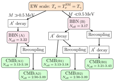
Figure 1: Possible cosmological histories of the active neutrinos $\nu_{a}$, the sterile neutrinos $\nu_{s}$, and the sterile sector gauge bosons $A^{\prime}$ below the electroweak (EW) scale. Various possibilities, labeled as A1, A2 and B1, B2, B3, are determined by the values of the $A^{\prime}$ mass $M$ and the $U(1)_{s}$ fine structure constant $\alpha_{s}$ and lead to testable predictions for $N_{\text{eff}}$ at both the BBN and CMB epochs. See text for details.

In Fig. 1, these two cases are summarized as BBN (A) and BBN (B), respectively. In either case, $N_{\text{eff,BBN{\tiny(A/B)}}}$ remains consistent with the current BBN bound on extra radiation, $\Delta N_{\text{eff,BBN}}=0.66^{+0.47}_{-0.45}$ (68% C.L.) Steigman:2012ve .

After BBN, the next important event is a possible secret recoupling of $\nu_{a}$ and $\nu_{s}$. If the sterile neutrino production rate $\Gamma_{s}>H$, a new hotter population of $\nu_{s}$ can be collisionally produced from $\nu_{a}$, and they achieve kinetic equilibrium with the primordially produced colder population of $\nu_{s}$. Also, the $A^{\prime}$ can decay and heat up the sterile neutrinos. Both processes change the number and energy density of neutrinos, and $N_{\rm eff}$ at CMB depends on the order in which they occur.

In Fig. 2, we show the collisional $\nu_{a}\rightarrow\nu_{s}$ production rate $\Gamma_{s}$, normalized to the Hubble expansion rate $H$, as a function of the photon temperature $T_{\gamma}$: $\Gamma_{s}/H$ is suppressed at high temperatures (say, above GeV), where $\sin^{2}2\theta_{m}$ is small due to the large $V_{\text{eff}}$. Since $\Gamma_{s}\propto T_{\gamma}^{-3}$ in this regime (see Eqs. (4), (5) and (9)) and $H\propto T_{\gamma}^{2}$, $\Gamma_{s}/H$ increases with $T_{\gamma}^{-5}$ as the temperature decreases. We define the recoupling temperature $T_{\text{re}}$ as the temperature where $\Gamma_{s}/H>1$ for the first time since the primordial decoupling of the active and sterile sectors above the QCD phase transition. When $T_{s}\sim M$, the energy and temperature dependence of $\Gamma_{s}$ changes (see Eq. (9)), and when also $V_{\text{eff}}$ drops below $\Delta m^{2}/(2T_{s})$ at $T_{s}<M$, $\Gamma_{s}$ begins to drop again. The asymptotic behavior is $\Gamma_{s}/H\propto T_{\gamma}^{3}$ at $T_{s}\ll M$ and $\theta_{m}\simeq\theta_{0}$. There are then three possible sequences of events:

1. No recoupling: For a sufficiently small interaction strength $\alpha_{s}$, the scattering rate $\Gamma_{s}$ always stays below the Hubble rate and there is no recoupling (solid black curve in Fig. 2).

If the interaction is stronger, a recoupling of $\nu_{a}$ and $\nu_{s}$ can happen either after or before $A^{\prime}$ decay:

1. Recoupling after $A^{\prime}$ decay: If $M>\text{few}\times 10^{-2}$ MeV, the recoupling happens after $A^{\prime}$ have decayed (dotted blue curve in Fig. 2).

2. Recoupling before $A^{\prime}$ decay: If $M<\text{few}\times 10^{-2}$ MeV, the recoupling happens before $A^{\prime}$ have decayed (dashed red curve in Fig. 2).

In the second and third cases, there is also a secret decoupling when $\Gamma_{s}/H$ again drops below one. If $e_{s}^{2}/M^{2}\leq{\cal O}(10\ \text{MeV}^{-2})$, this decoupling happens while $\nu_{s}$ are still relativistic, i.e. $T_{s}\gtrsim m_{s}/3$.

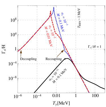
Figure 2: Evolution of the collisional $\nu_{a}\rightarrow\nu_{s}$ production rate $\Gamma_{s}$, normalized by the Hubble rate $H$, versus the photon temperature $T_{\gamma}$, for different representative choices of the secret gauge boson mass $M$ and the secret fine structure constant $\alpha_{s}$. When $\Gamma_{s}/H>1$, collisional production of $\nu_{s}$ from the thermal bath of $\nu_{a}$ is effective. The solid black curve shows a case where this never happens. The shoulder around $T_{\gamma}\sim M$ is where the $A^{\prime}$ decay away. The dotted blue and dashed red curves correspond to recoupling after and before $A^{\prime}$ decay, respectively.

In the following, we discuss the three aforementioned cases in detail.

III.0.1 No Recoupling

In the no recoupling cases, labeled as A1 and B1 in Fig. 1, the cosmological evolution after BBN is very straightforward. Vacuum oscillations convert a small fraction $\simeq\frac{1}{2}\sin^{2}2\theta_{0}\simeq 0.01$ of active neutrinos into sterile neutrinos (and vice versa), but this has negligible impact on the cosmological observables. Therefore, the temperature ratio $\xi$ at CMB can be derived from the separate conservation of entropy in the active neutrino sector and in the sterile neutrino sector. It is independent of when the $A^{\prime}$ decay (provided that it happens before the CMB epoch and approximately in chemical equilibrium.) That is, $\xi_{\text{CMB\tiny{A/B}}}\simeq\xi_{\text{BBN\tiny{(A)}}}=0.649$.

$N_{\text{eff,CMB}}$ can be estimated in analogy to Eq. (A). For the assumed sterile neutrino mass $\simeq 1$ eV, the $\nu_{s}$ contribution to the relativistic energy density has to be weighted by an extra factor because they are already semi-relativistic at the CMB epoch, where the photon temperature is $T_{\gamma}\simeq 0.30$ eV and the kinetic temperature of the sterile sector is $T_{s}=\xi_{\text{CMB}}\cdot(4/11)^{1/3}T_{\gamma}\simeq 0.14$ eV. As in Mirizzi:2014ama , we assume that the extra weight factor is characterized by the pressure $P$. (See Appendix A for the definition and calculations of the kinetic temperature and the pressure $P$ used here.) We thus obtain

$$N_{\text{eff,CMB}} =N_{\nu_{a}}+\frac{P_{m_{s}=\text{1\,eV}}}{P_{m_{s}=0}}\Bigg{|}_{\text{CMB}}\cdot\xi_{\text{CMB}}^{4}\simeq 3.13\,.$$ (18)

It is worth noting that the CMB temperature spectrum does not exactly measure the value of $N_{\text{eff,CMB}}$. Instead, the observed spectrum depends on the evolution of the energy density in relativistic degrees of freedom between the epoch of matter-radiation equality ($T_{\gamma,\text{eq}}\sim 0.7$ eV) and recombination ($T_{\gamma,\text{CMB}}\simeq 0.30$ eV) Planck:2015xua . Therefore, the value of $N_{\text{eff,CMB}}$ measured from the CMB temperature power spectrum lies between the values of $N_{\text{eff}}$ at $T_{\gamma,\text{CMB}}$ and $T_{\gamma,\text{eq}}$. The latter value, which we will denote by $N_{\text{eff,eq}}$, is given by

$$N_{\text{eff,eq}} =N_{\nu_{a}}+\frac{P_{m_{s}=\text{1\,eV}}}{P_{m_{s}=0}}\Bigg{|}_{\text{eq}}\cdot\xi_{\text{eq}}^{4}\simeq 3.18\,.$$ (19)

Both of these values agree with the bound from the 2015 Planck data release, $N_{\text{eff}}=3.15\pm 0.23$ (68% C.L.) Planck:2015xua .

III.0.2 Recoupling after $A^{\prime}$ decay

The cases of recoupling after $A^{\prime}$ decay are labeled as A2 and B2 in Fig. 1. In both cases, entropy conservation in the sterile sector before recoupling leads to a temperature ratio just after $A^{\prime}$ decay of $\xi_{M}\simeq\xi_{\text{BBN\tiny{(A)}}}=0.649$, which in turn implies

$$N_{\text{eff},M}=3.045+\xi^{4}_{M}=3.22\,.$$ (20)

Here, we have assumed that during $A^{\prime}$ decay chemical equilibrium holds in the sterile sector.

After recoupling, efficient neutrino oscillations and collisions lead to equilibration of the number densities and energy densities of all active and sterile neutrino species. Nevertheless, since number-changing interactions are strongly suppressed at $T_{s}\ll M$, this recoupling cannot change the total (active + sterile) neutrino number density and energy density beyond what is necessitated by cosmological expansion. The kinetic temperature $T_{\nu,\text{re}}$ shared by all neutrinos after recoupling is then given by

$$T_{\nu,\text{re}}\simeq\frac{3.045\cdot(T^{\text{SM}}_{\nu,\text{re}})^{4}+1\cdot T_{s,\text{re},0}^{4}}{3.045\cdot(T^{\text{SM}}_{\nu,\text{re}})^{3}+1\cdot T_{s,\text{re},0}^{3}}\simeq 0.97\,T^{\text{SM}}_{\nu}\,,$$ (21)

where $T^{\text{SM}}_{\nu}$ is the active neutrino temperature just prior to recoupling (which is at its SM value) and $T_{s,\text{re},0}$ denotes the sterile sector temperature just prior to recoupling.

Eventually, the mostly sterile eV-scale mass eigenstate decouples from the light mass eigenstates and becomes semi-relativistic at the CMB time. Its kinetic temperature at this epoch is $T_{s,\text{CMB}}\simeq 0.13$ eV. The effective number of relativistic species at the CMB epoch is given by

$$N_{\text{eff,CMB}} =N_{\text{eff,$M$}}\bigg{(}\frac{3}{4}+\frac{1}{4}\frac{P_{m_{s}=\text{1\,eV}}}{P_{m_{s}=0}}\bigg{|}_{\text{CMB}}\bigg{)}$$

$$\simeq 2.51+0.39\simeq 2.90\,.$$ (22)

Note that this is smaller than the SM value 3.045. This happens because part of the energy of active neutrinos has been transferred to the mostly sterile mass eigenstate $\nu_{4}$, whose kinetic energy gets redshifted away more efficiently after it becomes non-relativistic. Ref. Mirizzi:2014ama also found $N_{\text{eff}}<3$ for this scenario. Similarly, we obtain for the time of matter-radiation equality:

$$N_{\text{eff,eq}}=3.09\,.$$ (23)

Both values are in agreement with the Planck bound Planck:2015xua .

III.0.3 Recoupling before $A^{\prime}$ decay

The last possibility, labeled as case B3 in Fig. 1, is that recoupling happens before $A^{\prime}$ decay. In this case, all neutrinos, together with $A^{\prime}$, reach a common chemical equilibrium, which lasts until most of the $A^{\prime}$ particles have decayed. During the formation of chemical equilibrium, the total energy is conserved while entropy increases. Energy conservation allows us to calculate the temperature $T_{\nu,\text{re}}$ of the active + sterile neutrino sector immediately after recoupling:

$$(3g_{\nu_{a}}+g_{\nu_{s}}+g_{A^{\prime}})\,T_{\nu,\text{re}}^{4}\\ =\big{[}3g_{\nu_{a}}+(g_{\nu_{s}}+g_{A^{\prime}})\,\xi_{\text{BBN{\tiny(B)}}}^{4}\big{]}\,(T^{SM}_{\nu,\text{re}})^{4}\,,$$ (24)

where $T^{SM}_{\nu,\text{re}}$ is again the active neutrino temperature just prior to recoupling. Plugging in numbers for the effective numbers of degrees of freedom $g_{\nu_{a}}$, $g_{\nu_{s}}$, $g_{A^{\prime}}$ and using $\xi_{\text{BBN{\tiny(B)}}}=0.465$, we obtain

$$T_{\nu,\text{re}}=0.861\,T^{SM}_{\nu,\text{re}}\,.$$ (25)

Later, the $A^{\prime}$ decay and the thermal bath of neutrinos gets reheated by a factor $[(3g_{\nu_{a}}+g_{\nu_{s}}+g_{A^{\prime}})/(3g_{\nu_{a}}+g_{\nu_{s}})]^{1/3}\simeq 1.125$. The effective number of relativistic species after $A^{\prime}$ decay is then

$$N_{\text{eff},M}\simeq\frac{3g_{\nu_{a}}+g_{\nu_{s}}}{g_{\nu_{a}}}\,(1.125\cdot 0.861)^{4}\simeq 3.568.$$ (26)

The next steps are the decoupling of sterile neutrinos and active neutrinos, and then the freeze-out of sterile neutrino self-interactions. Since the number densities and energy densities of the different species do not change during these decouplings, the total effective number of relativistic degrees of freedom at the CMB epoch is given by

$$N_{\text{eff,CMB}} =N_{\text{eff,$M$}}\bigg{(}\frac{3}{4}+\frac{1}{4}\frac{P_{m_{s}=\text{1\,eV}}}{P_{m_{s}=0}}\bigg{|}_{\text{CMB}}\bigg{)}\simeq 3.21\,,$$ (27)

where again the pressure characterizes the contribution of the semi-relativistic $\nu_{4}$ to the radiation density in the Universe. Similarly, at matter-radiation equality we have

$$N_{\text{eff,eq}} \simeq 3.43\,.$$ (28)

This number is still within the $2\sigma$ error of the Planck bound Planck:2015xua .

IV Structure Formation

Besides the constraints on extra radiation measured by $N_{\text{eff}}$, CMB data also prefers that most of the active (massless) neutrinos start to free-stream before redshift $z\sim 10^{5}$ Archidiacono:2013dua ; Cyr-Racine:2013jua . On the other hand, matter power spectrum observations forbid these free-streaming degrees of freedom from carrying so much energy as to suppress small scale structures Lesgourgues:2012uu . Therefore measurements of the matter power spectrum put the most stringent upper bound on the mass of all fully thermalized neutrino species: $\sum m_{\nu}\lesssim 0.2$–$0.7$ eV (95% C.L.) Planck:2015xua . This concern Mirizzi:2014ama excludes a large proportion of the parameter region for self-interacting sterile neutrinos considered in Dasgupta:2013zpn . However, like the constraint on $N_{\text{eff}}$ discussed in Sec. III, it is avoided if $\Gamma_{s}$ never exceeds $H$ after the epoch when $V_{\text{eff}}$ drops below the oscillation frequency (cases A1 and B1 in Fig. 1).

Interestingly, structure formation constraints are also significantly relaxed when the $U(1)_{s}$ gauge coupling $e_{s}$ is large and/or the gauge boson mass $M$ is small. In this case, sterile neutrinos, although produced abundantly through collisional production (see Sec. II), cannot free-stream until late times, long after matter-radiation equality. Thus, their influence on structure formation is significantly reduced. We will now discuss this observation in more detail.

After the active and sterile neutrinos have equilibrated through $A^{\prime}$-mediated collisions, they should be treated as an incoherent mixture of the four mass eigenstates $\nu_{i}$ ($i=1\dots 4$). The reason is that for $m_{4}\sim 1$ eV, their oscillation time scales are much smaller than both the Hubble time and the time interval between scatterings. For simplicity, assume that only the mostly sterile mass eigenstate $\nu_{4}$ is massive with mass $m_{4}\simeq 1$ eV, and that it only mixes appreciably with one of the mostly active mass eigenstates, say $\nu_{1}$:

$$\nu_{s}\simeq\sin\theta_{0}\,\nu_{1}+\cos\theta_{0}\,\nu_{4}\,.$$ (29)

We take the vacuum mixing angle to be $\theta_{0}\simeq 0.1$ and we take into account that matter effects are negligible at temperatures relevant for structure formation (after matter–radiation equality). Since it is the flavor eigenstate $\nu_{s}$ that is charged under $U(1)_{s}$, the mass eigenstates $\nu_{1}$ and $\nu_{4}$ interact with relative rates $\sin^{2}\theta_{0}$ and $\cos^{2}\theta_{0}$, respectively, while $\nu_{2}$ and $\nu_{3}$ essentially free-stream.

To study the influence of the secret interaction on structure formation, we estimate the mean comoving distance $\lambda_{s}$ that each $\nu_{4}$ can travel in the early Universe. Since neutrinos can transport energy efficiently over scales smaller than $\lambda_{s}$, the matter power spectrum will be suppressed on these scales. As long as neutrinos are collisional, they do not free stream, but diffuse over scales of order Kolb:1988aj

$$(\lambda_{s}^{\text{coll}})^{2}\simeq\int_{0}^{t_{s}^{\text{dec}}}\!dt\,\frac{\langle v_{s}\rangle^{2}}{a^{2}(t)}\,\frac{1}{n_{s}\,\langle\sigma v\rangle_{s}}\,,$$ (30)

where $a(t)$ is the scale factor of the Universe, $t_{s}^{\text{dec}}$ is the time at which sterile neutrino self-interactions decouple,

$$\langle\sigma v\rangle_{s}\sim\langle v_{s}\rangle\frac{e_{s}^{4}\cos^{2}\theta_{0}}{(M^{2}+T_{s}^{2})^{2}}\,(T_{s}+m_{s})^{2}$$ (31)

is the thermally averaged interaction cross section of the mostly sterile mass eigenstate $\nu_{4}$, estimated here by naïve dimensional analysis, and $n_{s}$ is the number density of sterile neutrinos. For simplicity, we take the kinetic temperature $T_{s}$ of the sterile sector equal to the active neutrino temperature in this section, i.e. $T_{s}=T_{\nu}^{\text{SM}}=(4/11)^{1/3}T_{\gamma}\propto a^{-1}(t)$, as long as $\nu_{4}$ are relativistic. If sterile neutrinos become non-relativistic ($T_{s}<m_{s}$) while they are still strongly self-coupled, the kinetic temperature of the sterile sector scales as $T_{s}\propto a^{-2}(t)$ until $T_{s}$ drops below $T_{s,\text{dec}}$. After that, the sterile neutrino momenta are simply redshifted proportional to $a^{-1}(t)$. This implies in particular that, at $T_{s}\gg m_{s}$, we have $n_{s}\simeq T_{s}^{3}$, while after $\nu_{4}$ become non-relativistic, but are still strongly coupled, this changes to $n_{s}\propto T_{s}^{3/2}$. The computation of the average velocity $\langle v_{s}\rangle$ of $\nu_{4}$ entering eq. (31) is discussed in Appendix A.

The decoupling temperature $T_{s,\text{dec}}$ and the corresponding time $t_{s}^{\text{dec}}$ are defined by the condition that the sterile neutrino interaction rate is just equal to the Hubble rate:

$$n_{s}\,\langle\sigma v\rangle_{s}\big{|}_{t=t^{\text{dec}}}=H(t^{\text{dec}})\,.$$ (32)

After $t^{\text{dec}}$, sterile neutrinos start to free stream. The total comoving distance that a $\nu_{4}$ travels between the time $t^{\text{dec}}$ and the present epoch $t^{0}$ is Kolb:1988aj

$$\lambda^{\text{fs}}_{s}=\int_{t^{\text{dec}}}^{t_{0}}\!dt\,\frac{\langle v_{s}(t)\rangle}{a(t)}\,.$$ (33)

The overall damping scale is then given by

$$\lambda_{s}^{2}=(\lambda_{s}^{\text{coll}})^{2}+(\lambda^{\text{fs}}_{s})^{2}$$ (34)

At scales larger than $\lambda_{s}$, structure formation is unaffected by the existence of sterile neutrinos, while at smaller scales, structures are washed out.

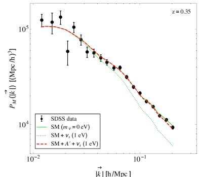
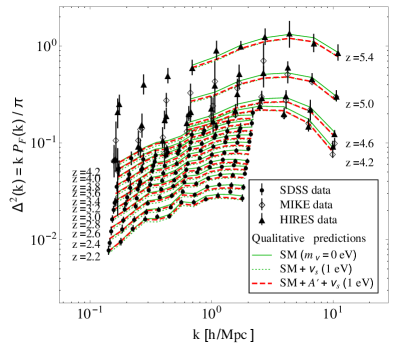
(a)	(b)

Figure 3: (a) Three-dimensional matter power spectrum $P_{M}(|\vec{k}|)$ derived from the SDSS Luminous Red Galaxy (LRG) Sample Tegmark:2006az and (b) one-dimensional flux power spectrum $\Delta^{2}(k)=k\,P_{F}(k)/\pi$ of Lyman-$\alpha$ photons at various redshifts, compared to the qualitative predictions of sterile neutrino models with (red dashed curves) and without (green dotted curves) self-interactions. Note that the relation between $P_{M}(|\vec{k}|)$ and $P_{F}(k)$ is non-linear, see e.g. Rossi:2014wsa . The assumed self-interaction parameters are $e_{s}=0.1$, $M=0.1$ MeV, and the assumed sterile neutrino mass is 1 eV. The data points and the SM prediction (solid green curves) are taken from Tegmark:2006az and and from Viel:2013fqw , respectively. The predictions including sterile neutrinos are obtained by multiplying the SM predictions by the $k$-dependent suppression profile from Fig. 7 of Lesgourgues:2012uu , shifted such that the onset of the suppression is at our calculated damping scale $k_{s}$ (Eq.(36); see text for details), and scaled such that the maximum suppression is given by Eq. (38) for panel (a) and by (39) for panel (b). Note that the error bars shown here are statistical only, and large systematic uncertainties, especially at small scales (large $k$) should be kept in mind.

As a numerical example, for $M=0.1\,\text{MeV}$, $e_{s}=0.1$, we find $\lambda_{s}^{\text{coll}}\simeq 29\leavevmode\nobreak\ \text{Mpc}/h$, $\lambda^{\text{fs}}_{s}\simeq 68\leavevmode\nobreak\ \text{Mpc}/h$ and thus

$$\lambda_{s}\simeq 74\leavevmode\nobreak\ \text{Mpc}/h\,,$$ (35)

corresponding to a wave number of

$$k_{s}\equiv 2\pi/\lambda_{s}\simeq 0.085\leavevmode\nobreak\ h/\text{Mpc}\,.$$ (36)

This should be compared to the free streaming scale of a decoupled sterile neutrino with a mass $\lesssim 1$ eV,

$$k_{s}^{\text{no self-int.}}\simeq 0.018\,\sqrt{m\over\text{eV}}\,h/\text{Mpc}\,.$$ (37)

This factor of $\sim 5$ decrease in the free streaming scale compared to a conventional sterile neutrinos without self-interactions implies that data on large scale structure (LSS) and baryon acoustic oscillations (BAO) will be in much better agreement with our model than with sterile neutrino models that do not feature self-interactions. The strongest constraints will come from data probing very small scales, in particular Lyman-$\alpha$ forests.

Even at scales $k>k_{s}$, the suppression of the matter power spectrum $P_{M}(|\vec{k}|)$ does not set in abruptly, but increases gradually. For non-interacting sterile neutrinos, numerical simulations show that the suppression saturates at $k\simeq 50\,k_{s}$. At even smaller scales (even larger $k$), the deviation from the prediction of standard cosmology is Lesgourgues:2006nd ; Lesgourgues:2012uu

$$\frac{\delta P_{M}(|\vec{k}|)}{P_{M}(|\vec{k}|)}\simeq-8f_{\nu}$$ (38)

in the linear structure formation regime. Here, $f_{\nu}=3m_{s}\zeta(3)/(2\pi^{2})\,T_{s}^{3}(t_{0})\times 8\pi G/(3H^{2}(t_{0}))/\Omega_{m}\simeq 0.07$ is the ratio of the sterile neutrino mass density $\Omega_{s}$ to the total mass density $\Omega_{m}\simeq 0.3$ today. In the regime of non-linear structure formation, $\delta P_{M}(|\vec{k}|)/P_{M}(|\vec{k}|)$ is somewhat larger Lesgourgues:2006nd ; Lesgourgues:2012uu , but N-body simulations show that it decreases again at scales $k\gtrsim\text{few}\leavevmode\nobreak\ h/\text{Mpc}$ Brandbyge:2008rv ; Rossi:2014wsa .

It is, however, difficult to directly measure $P_{M}(|\vec{k}|)$ at these nonlinear scales. The most sensitive data sets are Lyman-$\alpha$ forests, from which the 1-dimensional flux power spectrum $P_{F}(k)$ of Lyman-$\alpha$ photons can be extracted. Translating $P_{F}(k)$ into a measurement of $P_{M}(|\vec{k}|)$ requires a determination of the bias $b(k)$, which is obtained from numerical simulations of structure formation that include the dynamics of the gas clouds in which Lyman-$\alpha$ photons from distant quasars are absorbed. For SM neutrinos, such simulations have been performed for instance in Rossi:2014wsa , and we can estimate from Fig. 13 of that paper that the maximal suppression of $P_{F}(k)$ is of order

$$\frac{\delta P_{F}(k)}{P_{F}(k)}\sim-0.1\times\bigg{(}\frac{\sum m_{\nu}}{1\ \text{eV}}\bigg{)}\,,$$ (39)

where $\sum m_{\nu}$ is the sum of all neutrino masses. This estimate is crude but conservative, and ignores the fact that the maximal suppression is actually smaller at lower redshifts. The suppression of $P_{F}(k)$ described by Eq. (39) is smaller than the suppression of $P_{M}(|\vec{k}|)$ from Eq. (38) because of the nonlinear $k$-dependent relation between the matter power spectrum and the flux power spectrum (see for instance Croft:2000hs , especially Fig. 16 in that paper). Since no dedicated simulations are available for our self-interacting sterile neutrino model, we will assume in the following that $\delta P_{F}(k)/P_{F}(k)$ saturates at the value given by Eq. (39) even when $\sum m_{\nu}$ is dominated by the sterile neutrino mass $m_{s}$. This amounts to assuming that the impact of secretly interacting sterile neutrinos on these small scales is qualitatively similar to that of active neutrinos. A more detailed treatment requires a dedicated simulation including these secretly interacting sterile neutrinos. Note that neutrino free-streaming after CMB decoupling may lead to less suppression than described in Eqs. (38) and (39) because perturbation modes well within the horizon have already grown significantly by that time. We will not include this effect in the following discussion to remain conservative.

We show the qualitative impact of self-interacting sterile neutrinos on large scale structure in Fig. 3. Panel (a) compares theoretical predictions in models with and without sterile neutrinos to data on the three-dimensional matter power spectrum $P_{M}(|\vec{k}|)$ from the Sloan Digital Sky Survey (SDSS) Luminous Red Galaxy (LRG) catalog Tegmark:2006az . Panel (b) compares to one-dimensional flux power spectra $\Delta^{2}(k)\equiv k\,P_{F}(k)/\pi$ from Lyman-$\alpha$ forest data Viel:2013fqw . SDSS-LRG data corresponds to a mean redshift of $z\simeq 0.35$, while Lyman-$\alpha$ data is split up according to redshift and reaches up to $z\simeq 5.4$. Note that the data in Viel:2013fqw is presented as a function of the wave number $k_{v}$ in velocity space, measured in units of sec/km. The conversion to the wave number $k$ in coordinate space, measured in units of $h/\text{Mpc}$, is done according to the formula $k=k_{v}\,H(z)/(1+z)$, where $H(z)$ is the Hubble rate at redshift $z$. The theoretical predictions for the SM with vanishing neutrino mass (solid green curves in Fig. 3) are taken from Tegmark:2006az and Viel:2013fqw , respectively. Our (qualitative) predictions for sterile neutrino models with and without self-interactions are obtained in the following way: we start from the numerical prediction for the neutrino-induced suppression of the matter power spectrum from Ref. Lesgourgues:2012uu . In particular, we use the curve corresponding to $f_{\nu}=0.07$ from Fig. 7 in that paper. We then shift this curve such that the onset of the suppression coincides with our calculated damping scale $k_{s}$, and we rescale it such that the maximal suppression is $-8f_{\nu}$ in Fig. 3 (a) (linear regime) and 10% in Fig. 3 (b) (nonlinear regime), see Eqs. (38) and (39). We then multiply with the SM prediction to obtain the dotted green curves for sterile neutrinos without self-interactions and the red dashed curves for sterile neutrinos with self-interactions in Fig. 3. We use $e_{s}=0.1$, $M=0.1$ MeV and $m_{s}=1$ eV. Since we neglect a possible upturn of the power spectrum at $k\gtrsim 1\leavevmode\nobreak\ h/\text{Mpc}$ Brandbyge:2008rv , our estimates are very conservative.

From Fig. 3 (a), we observe that the suppression of the matter power spectrum at scales $\lesssim 0.2\leavevmode\nobreak\ h$/Mpc due to self-interacting sterile neutrinos is completely negligible, while a fully thermalized non-interacting sterile neutrino with the same mass leads to a clear suppression already at these scales. This implies that self-interacting sterile neutrinos with the parameters chosen here are not constrained by data on linear structure formation. Going to smaller scales or larger $k$ (Fig. 3 (b)), where non-linear effects become relevant, we see that both the sterile neutrino model with self-interactions and the one without lead to suppression, but the amount of suppression is reduced in the self-interacting case. It was shown in Ref. Viel:2013fqw that the data disfavors suppression larger than 10% at $k=10\,h/\text{Mpc}$. Self-interacting sterile neutrinos at the benchmark point shown in Fig. 3 appear to be marginally consistent with this constraint. It should be kept in mind, however, that our predictions are only qualitative. Therefore, only a detailed fit using simulations of non-linear structure formation that include sterile neutrino self-interactions could provide a conclusive assessment of the viability of such a scenario.

Let us finally discuss how the cosmological effects of the three active neutrinos are modified in the self-interacting sterile neutrino scenario. The dynamics of the mass eigenstates $\nu_{2}$ and $\nu_{3}$, which we assume not to mix with $\nu_{4}$, is the same as in standard cosmology: they start to free stream at redshift $z\gg 10^{5}$. $\nu_{1}$, however, starts to free stream later than a non-interacting neutrino, but earlier than $\nu_{4}$. The free-streaming condition for $\nu_{1}$ is, in analogy to Eq. (32),

$$(T_{\nu}^{\text{SM}})^{3}\cdot(T_{\nu}^{\text{SM}})^{2}\bigg{(}{e_{s}^{2}\over M^{2}}\bigg{)}^{2}\sin^{2}\theta_{0}\lesssim H\,.$$ (40)

As shown in Ref. Cyr-Racine:2013jua , free-streaming of active neutrinos before redshift $z\sim 10^{5}$ is required to sufficiently suppress the acoustic peaks in the CMB power spectrum. The change from three to two truly free streaming neutrino species in our model will lead to minor modifications of the CMB power spectrum, but the analysis from Cyr-Racine:2013jua suggests that these are unlikely to spoil the fit to CMB data, in particular since they may be compensated by changes in the best fit values of other cosmological parameters.

Note that also Planck CMB data alone, without including data on large scale structure observations, imposes an upper limit on the mass of sterile neutrinos, which, for a fully thermalized species is $m_{s}\lesssim 0.5$ eV at 95% C.L. Planck:2015xua . A much weaker bound is expected if self- interactions among sterile neutrinos are so strong that they remain collisional until after the CMB epoch. In this case, the early Integrated Sachs-Wolfe (ISW) effect induced by $\nu_{s}$ perturbations at low multipole order ($50\leq l\leq 200$) will be suppressed Lesgourgues:2012uu . Thus, the main effect on the CMB will come from the shift of matter–radiation equality, to which the sensitivity is, however, much weaker.

V Discussion and conclusions

As we have seen in the previous section, there are two main scenarios in which self-interacting sterile neutrinos do not run into conflict with cosmological data:

(i) The $\nu_{s}$ production rate $\Gamma_{s}$ drops below the Hubble expansion rate $H$ before the effective potential $|V_{\text{eff}}|$ drops below the oscillation frequency $|\Delta m^{2}/(2E)|$ and the dynamic suppression of active–sterile mixing due to $V_{\text{eff}}$ ends. In this case, sterile neutrinos are not produced in significant numbers in the early Universe and hence cosmology is not sensitive to their existence. An explanation of small scale structure anomalies as advocated in Dasgupta:2013zpn is, however, not possible in this scenario. In particular, even if the new interaction also couples to dark matter as proposed in Dasgupta:2013zpn , it is too weak to have phenomenological consequences.

This disadvantage can be avoided if more than one self-interacting sterile neutrino exists. Consider for example, a model with three mostly sterile neutrino mass eigenstates $\nu_{4}$, $\nu_{5}$, $\nu_{6}$. Let $\nu_{4}$ and $\nu_{5}$ have a relatively large mixing $\theta_{0}\sim 0.1$ with active neutrinos, as motivated for instance by the short baseline oscillation anomalies. Let their coupling to the $A^{\prime}$ gauge boson be $e_{s}^{(4,5)}\simeq 10^{-5}$, large enough to dynamically suppress their mixing with the mostly active mass eigenstates until after BBN, but small enough to prevent their equilibration afterwards. On the other hand, let $\nu_{6}$ have a vanishing mixing with $\nu_{1,2,3}$, but a larger secret gauge coupling $e_{s}^{(6)}\simeq 0.1$. Due to its small mixing, it is never produced through oscillations. However, its primordial population—the relic density produced before the visible and sterile sectors decoupled in the very early Universe—still acts as a thermal bath to which the dark matter may be strongly coupled, thus potentially solving the missing satellites problem Klypin:1999uc ; Boehm:2000gq ; Bringmann:2006mu ; Aarssen:2012fx ; Shoemaker:2013tda .

(ii) The self-interactions are so strong that sterile neutrinos remain collisional at least until matter–radiation equality. In this scenario, sterile neutrinos are produced when $|V_{\text{eff}}|\leq|\Delta m^{2}/(2E)|$. However, as shown in Sec. III, the effective number of relativistic degrees of freedom in the Universe, $N_{\text{eff}}$, remains close to 3 because equilibration between active and sterile neutrinos happens after neutrinos have decoupled from the photon bath. Moreover, as argued in Sec. IV, the impact of self-interacting sterile neutrinos on structure formation is much smaller in this scenario than the impact of conventional non-interacting sterile neutrino because they cannot transport energy efficiently over large distances due to their reduced free-streaming. Structure formation constraints could be further relaxed in models containing, besides an eV-scale mass eigenstate $\nu_{4}$, one or more additional mostly sterile states with much lower masses Tang:2014yla . It is intriguing that the parameter region corresponding to scenario (ii) contains the region where small scale structure anomalies can be explained, as shown in Dasgupta:2013zpn .

We summarize these results in Fig. 4. The yellow cross-hatched region on the right is ruled out because active and sterile neutrinos come into thermal equilibrium before the active neutrino decoupling from the SM plasma. In the lower part of this region, this happens simply because $V_{\text{eff}}$ is negligibly small. In the upper part, $V_{\text{eff}}$ is large, but also $\Gamma_{s}$ is large so that collisional production of sterile neutrinos is efficient in spite of the suppressed in-medium mixing $\theta_{m}$. This leads to constraints from $N_{\text{eff}}$ and from the light element abundances in BBN Saviano:2014esa . In the blue vertically hatched region, sterile neutrinos are produced after $\nu_{a}$ decoupling, so that CMB constraints on $N_{\text{eff}}$ remain satisfied. However, sterile neutrinos free-stream early on in this region and violate the CMB and structure formation constraints on their mass. This mass constraint can be considerably relaxed if the sterile neutrinos remain collisional until after the CMB epoch at $T_{\gamma}\simeq 0.3$ eV. This defines the upper edge of the blue hatched region. In the red shaded region in the upper left corner, the secret interaction is too strong and $\nu_{1}$ free streams too late. CMB data requires that active neutrinos free stream early enough, and thus strongly disfavors this region. Two white regions remain allowed: Scenario $(i)$ with weak self-interactions, corresponds to the wedge-shaped white region in the lower part of the plot. Scenario $(ii)$, with strong self-interactions, is realized in the thin white band between the blue vertically hatched region and the red shaded region. As explained above, whether or not this white band is allowed depends strongly on systematic uncertainties at Lyman-$\alpha$ scales and on the possible existence of additional states with masses $\ll 1$ eV.

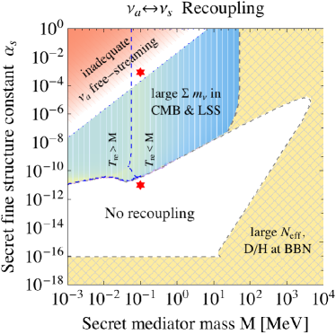
Figure 4: Schematic illustration of the parameter space for eV-scale sterile neutrinos coupled to a new “secret” gauge boson with mass $M$ and a secret fine structure constant $\alpha_{s}$. The vacuum mixing angle between active and sterile neutrinos was taken to be $\theta_{0}=0.1$. The white region in the lower half of the plot is allowed by all constraints, while the narrow white band in the upper left part satisfies all constraints except possibly large scale structure (LSS) limits from Lyman-$\alpha$ data at the smallest scales. The red stars show representative models in scenarios (i) and (ii). The colored regions are excluded, either by LSS observations (blue vertically hatched), by the requirement that active neutrinos should free stream early enough (red shaded), or by a combination of CMB and BBN data (yellow cross-hatched).

There are several important caveats and limitations to the above analysis. First, we have only worked with thermal averages for the parameters characterizing each particle species, such as energy, velocity, pressure, etc. To obtain more accurate predictions, it would be necessary to solve momentum-dependent quantum kinetic equations. This would be in particular interesting in the temperature regions where $V_{\text{eff}}$ changes sign and where $V_{\text{eff}}\sim\Delta m^{2}/(2T_{\nu_{a}})\times\cos 2\theta_{0}$. We expect that our modeling of flavor conversions in this region as fully non-adiabatic transitions is accurate, but this assumption remains to be checked explicitly. Moreover, the impact of self-interacting sterile neutrinos on non-linear structure formation at the smallest scales probed by Lyman-$\alpha$ data should be calculated more carefully. Improving these issues is left for future work.

In conclusion, we have argued in this paper that self-interacting sterile neutrinos remain a cosmologically viable extension of the Standard Model. As long as the self-interaction dynamically suppresses sterile neutrino production until neutrinos decouple from the photon bath, the abundance produced afterwards is not in conflict with constraints on $N_{\text{eff}}$. Moreover, if the self-interaction is either weak enough for scattering to be negligible after the dynamic mixing suppression is lifted, or strong enough to delay free streaming of sterile neutrinos until sufficiently late times, also structure formation constraints can be avoided or significantly relaxed.

Appendix A Kinetic temperature and pressure

In the following, we give more details on the momentum distribution function $f(p,t)$ of sterile neutrinos $\nu_{s}$ after they have decoupled from all other particle species. $f(p,t)$ is essential in the calculation of the pressure $P$ in Sec. III and the average velocity $\langle v_{s}\rangle$ in Sec. IV.

Even when $\nu_{s}$ are decoupled from other particles, they may still couple to themselves via strong self-interactions. If the self-interaction conserves the number of particles, such as $\nu_{s}\nu_{s}\leftrightarrow\nu_{s}\nu_{s}$, it only maintains kinetic equilibrium, but not chemical equilibrium. Number conservation and entropy maximization force the $\nu_{s}$ momentum distribution function in kinetic equilibrium to take the form

$$f(p,t)=\frac{1}{e^{[E(p)-\mu_{s}(t)]/T_{s}(t)}+1}\,,$$ (41)

where $T_{s}(t)$ is defined as the kinetic temperature, $\mu_{s}(t)$ is the chemical potential, and $E(p)=(p^{2}+m_{s}^{2})^{1/2}$. Here and in the following, we use the definition $p\equiv|\vec{p}|$. Since we are interested in the evolution at relatively late times, when the sterile neutrino density is low compared to the density of a degenerate fermion gas and thus $\langle f(p,t)\rangle\ll 1$, the classical approximation

$$f(p,t)\simeq e^{-[E(p)-\mu_{s}(t)]/T_{s}(t)}$$ (42)

is adequate.

Our goal is to solve for the functions $T_{s}(t)$ and $\mu_{s}(t)$ with the initial condition of a relativistic thermal ensemble of sterile neutrinos. This means that, initially, $T_{s}=T_{i}\gg m_{s}$ and $\mu_{s}=0$ at $a=a_{i}$. Note that the sterile neutrino mass will lead to a non-zero $\mu_{s}$ soon after neutrinos go out of chemical equilibrium. Although it is difficult to analytically solve the corresponding Boltzmann equation, there are two conditions that can be used to numerically obtain $T_{s}$ and $\mu_{s}$ as functions of the scale factor $a(t)$. One is number conservation. The other is entropy conservation, which holds approximately for kinetic equilibrium in the classical limit Bernstein:1988bw .

The number density is

$$n_{s}(t) =\int\!\frac{d^{3}p}{(2\pi)^{3}}\,f(p,t)$$ (43)

and the classical entropy density is defined as

$$s_{s}(t)\equiv\int\!\frac{d^{3}p}{(2\pi)^{3}}\,f(p,t)\,[1-\ln f(p,t)]\,.$$ (44)

It is straightforward to obtain the asymptotic solutions Bernstein:1988bw

$$T_{s}(t) \propto\begin{cases}a^{-1}(t)&\text{for $T_{s}\gg m_{s}$}\\[5.0pt] a^{-2}(t)&\text{for $T_{s}\ll m_{s}$}\end{cases}\,$$ (45)

and

$$\mu_{s}(t) \propto\begin{cases}a(t)&\text{for $T_{s}\gg m_{s}$}\\[5.0pt] \text{const}&\text{for $T_{s}\ll m_{s}$}\end{cases}\,.$$ (46)

In the transition region $T_{s}\sim m_{s}$, the solution needs to be obtained numerically. The result is plotted in Fig. 5.

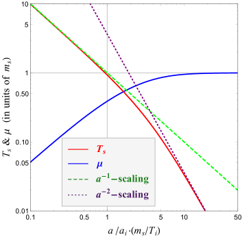
Figure 5: Kinetic temperature $T_{s}$ and chemical potential $\mu_{s}$ of sterile neutrinos, as functions of the scale factor $a(t)$ during the transition from the relativistic regime to the non-relativistic regime, with initial conditions $T_{s}=T_{i}\gg m_{s}$ and $\mu_{s}=0$ at $a=a_{i}$.

Finally, we comment on the calculation of the pressure $P$ and the average velocity $\langle v_{s}\rangle$ of sterile neutrinos. The pressure is given by Bernstein:1988bw

$$P \equiv\int\!\frac{d^{3}p}{(2\pi)^{3}}\,\frac{p^{2}}{3E}\,f(p,t)$$

$$=-T_{s}\,e^{\mu_{s}/T_{s}}\int\!\frac{d^{3}p}{(2\pi)^{3}}\,\frac{p}{3}\,\frac{d}{dp}e^{-E(p)/T_{s}}$$

$$=T_{s}\cdot n_{s}\,,$$ (47)

and the average velocity is

$$\langle v_{s}\rangle\simeq\frac{1}{N}\int\!\frac{d^{3}p}{(2\pi)^{3}}\frac{p}{E(p)}\,f(p,t)\,.$$ (48)

Here, $N\equiv\int\!dp\,4\pi p^{2}/(2\pi)^{3}\times f(p,t)$ is a normalization factor. Besides the conditions of kinetic equilibrium discussed above, we also need to take into account that sterile neutrino self-interactions freeze out at a time $t^{\text{dec}}$ and sterile sector temperature $T_{s}=T_{s,\text{dec}}$, after which kinetic equilibrium is lost and sterile neutrino momenta are simply redshifted as $a^{-1}(t)$. This implies for the momentum distribution function:

$$f(p,t)=\!\begin{cases}\frac{1}{\exp\!\big{[}\frac{1}{T_{s}(t)}\big{(}\sqrt{p^{2}+m_{s}^{2}}-\mu_{s}(t)\big{)}\big{]}+1}&\text{for $t<t^{\text{dec}}$}\\[11.38092pt] \frac{1}{\exp\!\big{[}\frac{1}{T_{s,\text{dec}}}\big{(}\sqrt{\frac{p^{2}a^{2}(t)}{a^{2}(t^{\text{dec}})}+m_{s}^{2}}-\mu_{s}(t^{\text{dec}})\big{)}\big{]}+1}&\text{for $t>t^{\text{dec}}$}\end{cases}\,.$$ (49)

Here, $\mu_{s}(t^{\text{dec}})$ is the chemical potential at the time of decoupling. We have checked that the exact decoupling time only slightly changes the evolution of $P$, so we regard our solution in Fig. 5 as universal for all parameter values of interest. In Sec. IV, we have for simplicity assumed a sudden decoupling of self-interactions though. For the value $e_{s}^{2}/M^{2}\simeq 1$ MeV^-2 chosen there, this leads to $T_{s,\text{dec}}\sim 0.0024$ eV, corresponding to a photon temperature of 0.038 eV.

References

- (1) LSND Collaboration, A. Aguilar et al., Evidence for neutrino oscillations from the observation of appearance in a beam, Phys. Rev. D64 (2001) 112007, [hep-ex/0104049].
- (2) MiniBooNE Collaboration, A. Aguilar-Arevalo et al., A Combined and Oscillation Analysis of the MiniBooNE Excesses, 1207.4809.
- (3) T. Mueller, D. Lhuillier, M. Fallot, A. Letourneau, S. Cormon, et al., Improved Predictions of Reactor Antineutrino Spectra, Phys.Rev. C83 (2011) 054615, [1101.2663].
- (4) G. Mention, M. Fechner, T. Lasserre, T. Mueller, D. Lhuillier, et al., The Reactor Antineutrino Anomaly, Phys.Rev. D83 (2011) 073006, [1101.2755].
- (5) A. Hayes, J. Friar, G. Garvey, G. Jungman, and G. Jonkmans, Systematic Uncertainties in the Analysis of the Reactor Neutrino Anomaly, Phys.Rev.Lett. 112 (2014) 202501, [1309.4146].
- (6) M. A. Acero, C. Giunti, and M. Laveder, Limits on nu(e) and anti-nu(e) disappearance from Gallium and reactor experiments, Phys.Rev. D78 (2008) 073009, [0711.4222].
- (7) J. Kopp, M. Maltoni, and T. Schwetz, Are there sterile neutrinos at the eV scale?, Phys.Rev.Lett. 107 (2011) 091801, [1103.4570].
- (8) J. Kopp, P. A. N. Machado, M. Maltoni, and T. Schwetz, Sterile Neutrino Oscillations: The Global Picture, JHEP 1305 (2013) 050, [1303.3011].
- (9) J. Conrad, C. Ignarra, G. Karagiorgi, M. Shaevitz, and J. Spitz, Sterile Neutrino Fits to Short Baseline Neutrino Oscillation Measurements, Adv.High Energy Phys. 2013 (2013) 163897, [1207.4765].
- (10) J. R. Kristiansen, . Elgarøy, C. Giunti, and M. Laveder, Cosmology with sterile neutrino masses from oscillation experiments, 1303.4654.
- (11) C. Giunti, M. Laveder, Y. Li, and H. Long, Pragmatic View of Short-Baseline Neutrino Oscillations, Phys.Rev. D88 (2013) 073008, [1308.5288].
- (12) G. Steigman, Neutrinos And Big Bang Nucleosynthesis, Adv.High Energy Phys. 2012 (2012) 268321, [1208.0032].
- (13) Planck Collaboration, P. Ade et al., Planck 2015 results. XIII. Cosmological parameters, 1502.01589.
- (14) J. Hamann, S. Hannestad, G. G. Raffelt, and Y. Y. Wong, Sterile neutrinos with eV masses in cosmology: How disfavoured exactly?, JCAP 1109 (2011) 034, [1108.4136].
- (15) S. Hannestad, R. S. Hansen, and T. Tram, How secret interactions can reconcile sterile neutrinos with cosmology, Phys.Rev.Lett. 112 (2014) 031802, [1310.5926].
- (16) B. Dasgupta and J. Kopp, Cosmologically Safe eV-Scale Sterile Neutrinos and Improved Dark Matter Structure, Phys.Rev.Lett. 112 (2014), no. 3 031803, [1310.6337].
- (17) T. Bringmann, J. Hasenkamp, and J. Kersten, Tight bonds between sterile neutrinos and dark matter, JCAP 1407 (2014) 042, [1312.4947].
- (18) P. Ko and Y. Tang, Self-interacting scalar dark matter with local symmetry, JCAP 1405 (2014) 047, [1402.6449].
- (19) K. C. Y. Ng and J. F. Beacom, Cosmic neutrino cascades from secret neutrino interactions, Phys.Rev. D90 (2014), no. 6 065035, [1404.2288].
- (20) J. Kopp and J. Welter, The Not-So-Sterile 4th Neutrino: Constraints on New Gauge Interactions from Neutrino Oscillation Experiments, JHEP 1412 (2014) 104, [1408.0289].
- (21) N. Saviano, O. Pisanti, G. Mangano, and A. Mirizzi, Unveiling secret interactions among sterile neutrinos with big-bang nucleosynthesis, Phys.Rev. D90 (2014), no. 11 113009, [1409.1680].
- (22) A. Mirizzi, G. Mangano, O. Pisanti, and N. Saviano, Collisional production of sterile neutrinos via secret interactions and cosmological implications, Phys.Rev. D91 (2015), no. 2 025019, [1410.1385].
- (23) J. F. Cherry, A. Friedland, and I. M. Shoemaker, Neutrino Portal Dark Matter: From Dwarf Galaxies to IceCube, 1411.1071.
- (24) C. Kouvaris, I. M. Shoemaker, and K. Tuominen, Self-Interacting Dark Matter through the Higgs Portal, Phys.Rev. D91 (2015), no. 4 043519, [1411.3730].
- (25) Y. Tang, More Is Different: Reconciling eV Sterile Neutrinos and Cosmological Mass Bounds, 1501.00059.
- (26) S. Dodelson and L. M. Widrow, Sterile-neutrinos as dark matter, Phys.Rev.Lett. 72 (1994) 17–20, [hep-ph/9303287].
- (27) L. Stodolsky, On the Treatment of Neutrino Oscillations in a Thermal Environment, Phys.Rev. D36 (1987) 2273.
- (28) T. D. Jacques, L. M. Krauss, and C. Lunardini, Additional Light Sterile Neutrinos and Cosmology, Phys.Rev. D87 (2013), no. 8 083515, [1301.3119].
- (29) F.-Y. Cyr-Racine and K. Sigurdson, Limits on Neutrino-Neutrino Scattering in the Early Universe, Phys.Rev. D90 (2014), no. 12 123533, [1306.1536].
- (30) M. Archidiacono and S. Hannestad, Updated constraints on non-standard neutrino interactions from Planck, JCAP 1407 (2014) 046, [1311.3873].
- (31) J. Lesgourgues and S. Pastor, Neutrino mass from Cosmology, Adv.High Energy Phys. 2012 (2012) 608515, [1212.6154].
- (32) E. W. Kolb and M. S. Turner, The Early Universe, .
- (33) SDSS Collaboration, M. Tegmark et al., Cosmological Constraints from the SDSS Luminous Red Galaxies, Phys.Rev. D74 (2006) 123507, [astro-ph/0608632].
- (34) G. Rossi, N. Palanque-Delabrouille, A. Borde, M. Viel, C. Yeche, et al., Suite of hydrodynamical simulations for the Lyman-α forest with massive neutrinos, Astron.Astrophys. 567 (2014) A79, [1401.6464].
- (35) M. Viel, G. D. Becker, J. S. Bolton, and M. G. Haehnelt, Warm dark matter as a solution to the small scale crisis: New constraints from high redshift Lyman-α forest data, Phys.Rev. D88 (2013) 043502, [1306.2314].
- (36) J. Lesgourgues and S. Pastor, Massive neutrinos and cosmology, Phys.Rept. 429 (2006) 307–379, [astro-ph/0603494].
- (37) J. Brandbyge, S. Hannestad, T. Haugbolle, and B. Thomsen, The Effect of Thermal Neutrino Motion on the Non-linear Cosmological Matter Power Spectrum, JCAP 0808 (2008) 020, [0802.3700].
- (38) R. A. Croft, D. H. Weinberg, M. Bolte, S. Burles, L. Hernquist, et al., Towards a precise measurement of matter clustering: Lyman alpha forest data at redshifts 2-4, Astrophys.J. 581 (2002) 20–52, [astro-ph/0012324].
- (39) M. Vogelsberger, S. Genel, V. Springel, P. Torrey, D. Sijacki, et al., Properties of galaxies reproduced by a hydrodynamic simulation, Nature 509 (2014) 177–182, [1405.1418].
- (40) T. Sawala, C. S. Frenk, A. Fattahi, J. F. Navarro, R. G. Bower, et al., Local Group galaxies emerge from the dark, 1412.2748.
- (41) A. A. Klypin, A. V. Kravtsov, O. Valenzuela, and F. Prada, Where are the missing Galactic satellites?, Astrophys.J. 522 (1999) 82–92, [astro-ph/9901240].
- (42) C. Boehm, P. Fayet, and R. Schaeffer, Constraining dark matter candidates from structure formation, Phys.Lett. B518 (2001) 8–14, [astro-ph/0012504].
- (43) T. Bringmann and S. Hofmann, Thermal decoupling of WIMPs from first principles, JCAP 0407 (2007) 016, [hep-ph/0612238].
- (44) L. G. van den Aarssen, T. Bringmann, and C. Pfrommer, Is dark matter with long-range interactions a solution to all small-scale problems of CDM cosmology?, Phys.Rev.Lett. 109 (2012) 231301, [1205.5809].
- (45) I. M. Shoemaker, Constraints on Dark Matter Protohalos in Effective Theories and Neutrinophilic Dark Matter, 1305.1936.
- (46) J. Bernstein, Kinetic Theory in the Expanding Universe, .