Magnetic field relaxation and current sheets in an ideal plasma

Abstract

We investigate the existence of magnetohydrostatic equilibria for topologically complex magnetic fields. The approach employed is to perform ideal numerical relaxation experiments. We use a newly-developed Lagrangian relaxation scheme that exactly preserves the magnetic field topology during the relaxation. Our configurations include both twisted and sheared fields, of which some fall into the category for which Parker (1972) predicted no force-free equilibrium. The first class of field considered contains no magnetic null points, and field lines connect between two perfectly conducting plates. In these cases we observe only resolved current layers of finite thickness. In further numerical experiments we confirm that magnetic null points are loci of singular currents.

1. Introduction

Magnetic field relaxation in environments like the solar atmosphere and laboratory plasma is a crucial process in understanding open problems like solar flares and field stability in tokamaks. In such environments the field evolves nearly ideally, i.e. the magnetic flux remains frozen to the plasma. For an arbitrary braided magnetic field between two perfectly conducting planes Parker (1972) hypothesized that there can be a force-free equilibrium of the same topology only if the field’s twist varies uniformly along the large-scale magnetic field. He further suggested that in resistive magnetohydrodynamics (MHD), where reconnection can occur, the field would then undergo a rapid change in topology accompanied by magnetic energy dissipation that would provide a significant contribution to coronal heating (Parker, 1983b).

In subsequent works this idea has been confirmed and challenged various times (Parker, 1983b; Craig & Sneyd, 2005; Low, 2010, 2013). Braided magnetic fields from foot point motions were shown to be complex enough that they must exhibit the proposed topological dissipation (Parker, 1983a). Low (2010) later showed that there exist solutions for the relaxing magnetic field which permit current sheets. One of the first simulations testing the conjecture was performed by Mikic et al. (1989) who found filamentary current structures with an exponentially increasing strength. Given the limited computing power of that time, they were only able to reach very moderate resolutions, which renders it questionable if they observed proper sheets.

Doubts about Parker’s conjecture came from e.g. van Ballegooijen (1985) who suggested that a field generated by foot point motions is able to adjust to those motions and reach a force-free state so long as the velocity field is continuous at the boundary. This was supported by later numerical simulations, in which a series of footpoint displacements were performed, and an exponential thinning and intensification of current layers was observed – rather than a collapse to sub-grid scale of the current (van Ballegooijen, 1988). It has also been suggested that in certain configurations no thin current layers – finite or infinite – need necessarily form. Craig & Sneyd (2005) derived solutions for relaxing magnetic fields which do not show singularities even with sufficiently braided configurations. However, Pontin & Hornig (2015) recently demonstrated that for any braided magnetic field in which the field line mapping exhibits small length scales, thin current layers are an inevitable feature of the corresponding force-free equilibrium, if it exists. Building on earlier work by Wilmot-Smith et al. (2009) they showed that the ideal relaxation of a class of braided fields leads to a current distribution of finite strength. Moreover, the current layers obtained in the approximate force-free equilibria were shown to scale in both thickness and intensity with length scales present in the field line mapping, consistent with the earlier results of van Ballegooijen (1988).

In this work we tackle the problem of current sheet formation during magnetic field relaxation for various topologically non-trivial configurations at unprecedented numerical resolution. Longcope & Strauss (1994) pointed out that there exist solutions for relaxed magnetic fields which have current layers thin enough that they cannot be distinguished from current sheets with moderate grid resolution. We apply the newly developed numerical code GLEMuR (Candelaresi et al., 2014) which uses the resources of graphical processing units (GPUs) and makes use of mimetic differential operators (Hyman & Shashkov, 1997), which greatly improve the relaxation quality. The scheme is Lagrangian, and is constructed in such a way that it perfectly preserves the magnetic topology (Craig & Sneyd, 1986).

Emphasis is put on braids which are not reducible to uniform twists along a mean magnetic field such as those used by Wilmot-Smith et al. (2009), as well as fields generated through footpoint motions such as those by Longbottom et al. (1998). We further investigate the effect of modifying the magnetic field to include magnetic null points, and show that current singularities form there (as in Pontin & Craig, 2005; Craig & Pontin, 2014).

2. Model and Methods

2.1. Ideal Evolution

In order to determine existence and structure of equilibria for given magnetic topologies, we require to follow an exactly ideal evolution. We employ a method that by its construction exactly preserves the magnetic flux, magnetic field line connectivity, and solenoidal nature of the magnetic field $\bm{B}$ during the relaxation. Specifically, we use the Lagrangian code GLEMuR (Candelaresi et al., 2014) which solves the equations for an ideal evolution of a magnetized non-Newtonian fluid without inertia, as well as an extension to this method that considers a damped fluid with inertia. These methods have computational advantages over those that solve for the full dynamics of ideal MHD, leading towards a minimum energy state whose properties are our main concern (rather than the evolution to reach the relaxed state).

In order to preserve the field’s topology we make use of a Lagrangian grid method where the grid points move along with the fluid. If the initial positions of fluid particles at time $t=0$ are described by the position vector field $\bm{X}$, we denote their position at time $t$ by $\bm{x}(\bm{X},t)$ with $\bm{x}(\bm{X},0)=\bm{X}$. These fluid elements (grid points) are evolved according to

$$\frac{\partial\bm{x}(\bm{X},t)}{\partial t}=\mbox{\boldmath$u$}{}(\bm{x}(\bm{X},t),t),$$ (1)

where the velocity $u$ is chosen in such a way to lead towards an equilibrium. We employ different methods for choosing $u$, as outlined below.

Any ideal evolution of the magnetic field $\bm{B}$ must be consistent with the ideal induction equation

$$\frac{\partial\bm{B}}{\partial t}-\mbox{\boldmath$\nabla$}{}\times(\mbox{\boldmath$u$}{}\times\bm{B})=0,$$ (2)

which implies that the magnetic field is frozen into the fluid (Batchelor, 1950; Priest & Forbes, 2000), i.e. moves together with the fluid particles. From the frozen in condition we can relate the magnetic field at later time (following a deformation of the fluid particle mesh) to the magnetic field at $t=0$;

$$B_{i}(\bm{X},t)=\frac{1}{\Delta}\sum_{j=1}^{3}\frac{\partial x_{i}}{\partial X_{j}}B_{j}(\bm{X},0),$$ (3)

with $B_{i}$ being the $i^{\rm th}$ component of the magnetic field and $\Delta=\det(\partial x_{i}/\partial X_{j})$ (Craig & Sneyd, 1986; Candelaresi et al., 2014). Here the fields are functions of their initial positions $\bm{X}$ and time $t$. In other words, they are functions of the fluid particle positions.

For some of the relaxation simulations described herein, we follow Candelaresi et al. (2014) by applying the magneto-frictional term (Chodura & Schlüter, 1981) for the evolution of the fluid

$$\mbox{\boldmath$u$}{}=\mbox{\boldmath$J$}{}\times\bm{B},$$ (4)

with the current density $\mbox{\boldmath$J$}{}=\mbox{\boldmath$\nabla$}{}\times\bm{B}$. This is the evolution equation for a non-Newtonian fluid without inertia, and the evolution terminates when a force-free field (satisfying $\mbox{\boldmath$J$}{}\times\bm{B}={\bf 0}$) is attained. This approach is well suited for studying relaxation problems, as it is shown to lead to a monotonic decay of the magnetic energy (Craig & Sneyd, 1986; Yang et al., 1986).

However, there are two disadvantages to this approach. First, the monotonic energy decay means that during the relaxation the system is unable to escape any small local energy minima if a lower global energy minimum exists. Second, in a magnetic field containing null points, the null point positions are fixed (since the $\mbox{\boldmath$J$}{}\times\bm{B}$ force at the nulls themselves must be zero). To address the first issue we consider an extension of the method that makes use of inertial effects. The fluid’s evolution equation is then given by

$$\frac{{\rm d}{}\mbox{\boldmath$u$}{}}{{\rm d}{}t}=(\mbox{\boldmath$J$}{}\times\bm{B}-\nu\mbox{\boldmath$u$}{})/\rho,$$ (5)

with the damping coefficient $\nu$ and density $\rho$.

To address the second issue of stationary magnetic null points we employ a pressure force. In some cases described below it is beneficial to seek an equilibrium that is not force-free, but where the Lorentz force is balanced by a pressure gradient. For simplicity here we assume that the pressure is directly proportional to the fluid density (corresponding to an ideal gas under isothermal changes of state). This yields an evolution of the fluid mesh

$$\mbox{\boldmath$u$}{}=\mbox{\boldmath$J$}{}\times\bm{B}-\beta\mbox{\boldmath$\nabla$}{}\rho,$$ (6)

with the compressibility parameter $\beta$. The density can be expressed in terms of the initial density $\rho_{0}$ as $\rho(\bm{x},t)=\rho_{0}/\Delta=\rho(\bm{X},0)/\Delta$, and for convenience we will always choose $\rho_{0}=1$. We can also add the pressure gradient to the inertial evolution equation, to give

$$\frac{{\rm d}{}\mbox{\boldmath$u$}{}}{{\rm d}{}t}=(\mbox{\boldmath$J$}{}\times\bm{B}-\nu\mbox{\boldmath$u$}{}-\beta\mbox{\boldmath$\nabla$}{}\rho)/\rho.$$ (7)

Computing spatial derivatives on a moving grid is a sensitive operation. The direct approach used in previous numerical implementations of the magneto-frictional approach involves application of the chain rule leading to expressions involving various products of derivatives (Craig & Sneyd, 1986). Using such direct derivatives for computing $\mbox{\boldmath$J$}{}=\mbox{\boldmath$\nabla$}{}\times\bm{B}$ on highly distorted grids, such as those we expect to occur in our numerical experiments, leads to numerical inaccuracies, most notably the issue that $\mbox{\boldmath$\nabla$}{}\cdot\mbox{\boldmath$J$}{}=0$ is not well fulfilled, as was noted by Pontin et al. (2009). Our code GLEMuR makes use of mimetic numerical operators to compute the curl, which have been shown to more accurately represent the current on such meshes, and have the advantage that they preserve the identity $\mbox{\boldmath$\nabla$}{}\cdot(\mbox{\boldmath$\nabla$}{}\times\bm{B})=0$ up to machine precision for some appropriate mimetic divergence operator (Hyman & Shashkov, 1997; Candelaresi et al., 2014). For the time stepping we use a Runge-Kutta 6th order in time approach.

All three boundary conditions can be chosen to be periodic or line-tied. Here line-tied means that the velocity is set to zero and the normal component of the magnetic field is fixed. For studying the problem proposed by Parker (1972) we will typically use such line-tied boundaries in the $z$ direction in the simulations described below. But occasionally we will impose periodic boundaries.

2.2. Diagnostic Parameters

Here we describe some diagnostic tools that are used in the following sections to analyse the properties of the final states of our relaxation simulations. The evolution of the system by equation (4) is solely determined by the Lorentz force $\mbox{\boldmath$F$}{}_{\rm L}=\mbox{\boldmath$J$}{}\times\bm{B}$. A force-free state implies $\mbox{\boldmath$F$}{}_{\rm L}=0$, which is equivalent to $\mbox{\boldmath$\nabla$}{}\times\bm{B}=\alpha\bm{B}$, where $\alpha$ is the force-free parameter which satisfies $\mbox{\boldmath$\nabla$}{}\alpha\cdot\bm{B}=0$, i.e. $\alpha$ is constant along magnetic field lines. During the relaxation simulations, the magnetic field evolves into an energetically more favorable state with approximately vanishing Lorentz force (when $\beta=0$). Since the Lorentz force never vanishes identically in this numerical approximation, the condition $\mbox{\boldmath$\nabla$}{}\times\bm{B}=\alpha\bm{B}$ is not fulfilled exactly either. We can, nevertheless, still express the curl of the magnetic field in terms of a component parallel and perpendicular to $\bm{B}$:

$$\mbox{\boldmath$\nabla$}{}\times\bm{B}=\lambda\bm{B}-\mbox{\boldmath$\epsilon$}{}\times\bm{B},$$ (8)

with the parameter $\lambda$ and vector $\epsilon$, where we choose $\epsilon$ such that $\mbox{\boldmath$\epsilon$}{}\cdot\bm{B}=0$. These two parameters are used to determine the deviation from the force-free state quantitatively.

From equation (8) we obtain

$$\lambda=\frac{\mbox{\boldmath$J$}{}\cdot\bm{B}}{\bm{B}^{2}},$$ (9)

$$\mbox{\boldmath$\epsilon$}{}=\frac{\mbox{\boldmath$J$}{}\times\bm{B}}{\bm{B}^{2}}.$$ (10)

Comparing $\lambda$ and $\epsilon$ for each field line we can infer to what degree the field is force-free. For that we need to trace magnetic field lines from the bottom of the domain at $z=Z_{0}$ to the top at $z=Z_{1}$ and integrate $\lambda$ and $|\mbox{\boldmath$\epsilon$}{}|$ along the lines $C$:

$$\lambda(X,Y)=\frac{1}{L}\int\limits_{C}\frac{\mbox{\boldmath$J$}{}\cdot\bm{B}}{\bm{B}^{2}}\ {\rm d}{}l,$$ (11)

$$\epsilon(X,Y)=\frac{1}{L}\int\limits_{C}\left|\frac{\mbox{\boldmath$J$}{}\times\bm{B}}{\bm{B}^{2}}\right|\ {\rm d}{}l,$$ (12)

$$L=\int\limits_{C}{\rm d}{}l,$$ (13)

where we start our field line integration at $(X,Y,Z_{0})$. The ratio $\epsilon(X,Y)/\lambda(X,Y)$ gives the relative deviation from the force-free state. Since $\bm{B}\cdot\mbox{\boldmath$\nabla$}{}\lambda=0$ for the force-free state we also compute the maximum slope of $\lambda$ along the field lines in analogy to Pontin et al. (2009) and Candelaresi et al. (2014):

$$\lambda^{*}(X,Y)=\max_{i}\left(\frac{\lambda_{i+1}-\lambda_{i}}{l_{i+1}-l_{i}}\right),$$ (14)

with the value $\lambda_{i}$ at point $i$ on the field line and the length of the field line $l$.

For magnetic field lines extending between two parallel planes Berger (1986) suggested a relation between magnetic helicity density and the winding of the field around itself. Because the magnetic helicity density $h_{\rm m}$ is defined via the magnetic vector potential $A$ we choose to measure the twist of the magnetic field lines by

$$\omega(X,Y)=\frac{1}{L}\int\limits_{C}\frac{\mbox{\boldmath$J$}{}\cdot\bm{B}}{|\mbox{\boldmath$J$}{}||\bm{B}|}\ {\rm d}{}l.$$ (15)

For a force-free field this expression reduces to $\omega(X,Y)={\rm sgn}\,{}(\alpha)$.

Wilmot-Smith et al. (2010) showed that magnetic field lines with a high integrated electric current are places of current sheet formation and hence reconnection. In our ideal simulations no reconnection can occur, but of course the formation of localized current concentrations may take place. To analyze their occurrence we compute the magnetic field line integrated current density

$$\mbox{\boldmath$J$}{}_{||}(X,Y)=\int\limits_{C}\frac{\mbox{\boldmath$J$}{}\cdot\bm{B}}{|\bm{B}|}\ {\rm d}{}l.$$ (16)

3. Braided Fields

From previous numerical experiments (Wilmot-Smith et al., 2009) we know that topologically complex braids do not necessarily form singular current sheets as the field relaxes towards a force-free state. Here we investigate the relaxation behavior of the magnetic braids discussed by e.g. Wilmot-Smith et al. (2009) and Yeates et al. (2010). To study the relaxation of these fields we use the magneto-frictional evolution given by Equation (4).

The initial magnetic field we consider is the one named $E^{3}$ by Wilmot-Smith et al. (2009), which consists of three braiding regions and a homogeneous background magnetic field such that $B_{z}>0$ everywhere. Its form is given by

$$\bm{B}_{\rm E^{3}}(0) =B_{0}\mbox{\boldmath$e$}{}_{z}+\sum_{c=1}^{6}\frac{2kB_{0}}{a}(-(y-y_{c})\mbox{\boldmath$e$}{}_{x}+(x-x_{c})\mbox{\boldmath$e$}{}_{y})$$ (17)

$$\times\exp\left(\frac{-(x-x_{c})^{2}-(y-y_{c})^{2}}{a^{2}}-\frac{(z-z_{c})^{2}}{l^{2}}\right),$$

with the initial field strength $B_{0}$, strength of twist $k$, radius and length in $z$-direction of the twist region $a$ and $l$ respectively and the twist locations $(x_{c},y_{c},z_{c})$. We choose $x_{c}=\{1,-1,1,-1,1,-1\}$, $y_{c}=0$, $z_{c}=\{-20,-12,-4,4,12,20\}$, $a=\sqrt{2}$, $l=2$ and $B_{0}=1$. To fit this configuration into a computational domain, the box size is chosen to extend 8 units in $x$ and $y$ and 48 units in $z$ centered at the origin. Upper and lower boundaries are chosen either to be line-tied or periodic and the grid resolution is $300$ in each direction. Sample magnetic field lines are shown in Figure 1.

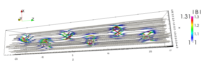
Figure 1.— Initial magnetic field lines for the $E^{3}$ configuration. Colors denote the field strength which is strongest in the twist regions.

3.1. Formation of Current Layers

As the field evolves and tries to minimize the magnetic energy it forms concentrations of strong currents. According to Parker (1972) singular current sheets should form. However, we do not find any such formation irrespective of the grid resolution (Figure 2, upper panel) and all current concentrations are well resolved which favors Ballegooijen’s result (van Ballegooijen, 1985). This is even true if we choose periodic boundaries in z-direction (Figure 2, lower panel).

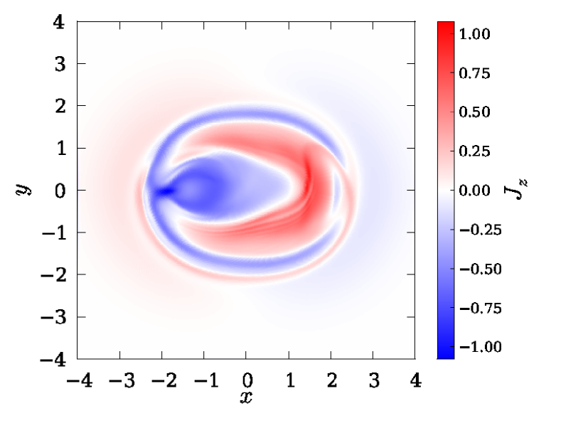
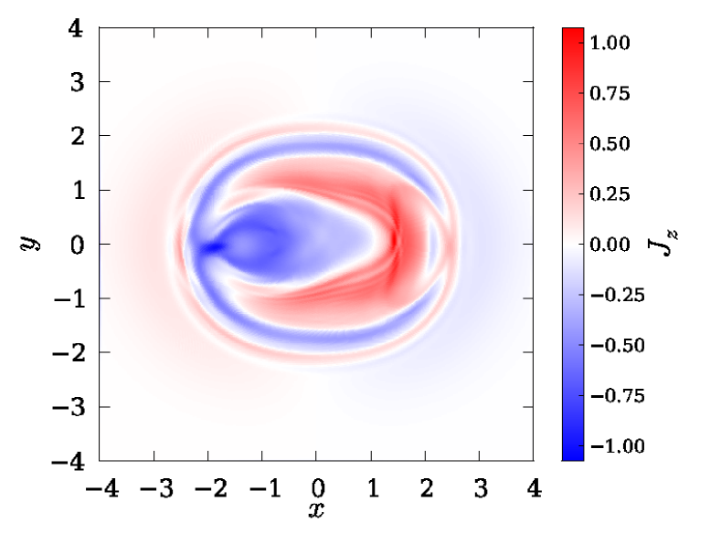
Figure 2.— $z$-component of the electric current density at $z=3.8$ for times close to relaxation for $E^{3}$ with line tied (upper panel) and periodic boundaries in z (lower panel).

Varying the grid resolution does not significantly change the outcome of these simulations. The width of the current layers remains the same, as well as the strength of the current.

3.2. Topological Complexity

Since the evolution of the magnetic field is ideal it preserves its topology and changes in connectivity are forbidden. One measure of the field’s topological complexity is the field line integrated electric current density $\mbox{\boldmath$J$}{}_{||}(X,Y)$. We observe an approximate conservation for $\mbox{\boldmath$J$}{}_{||}$ for our test configuration of $E^{3}$ (Figure 3).

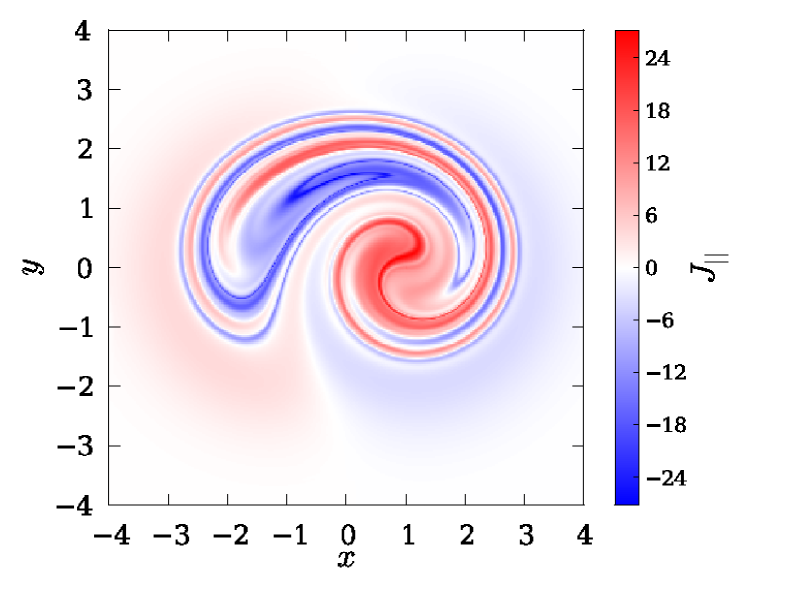
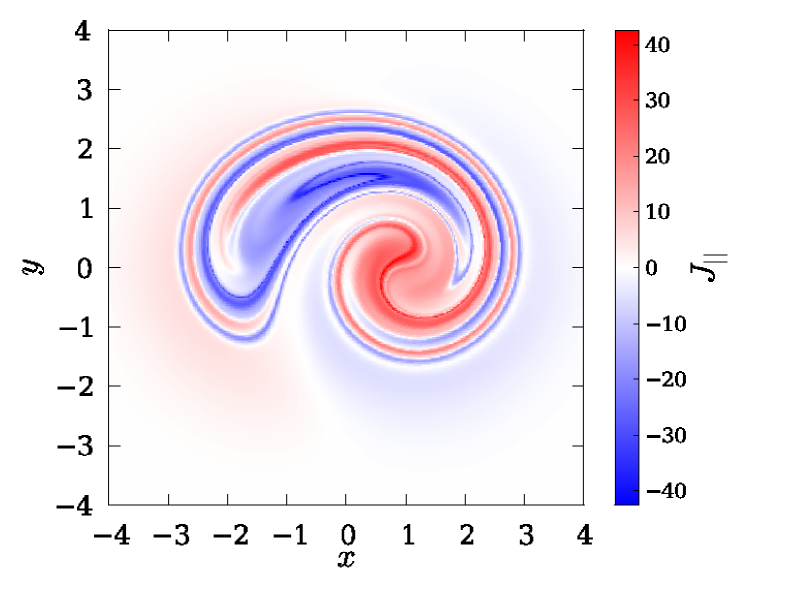
Figure 3.— Line integrated electric current density $J_{||}(X,Y)$ as computed from equation (16) for $E^{3}$ with line tied boundaries at initial time $t=0$ and time at relaxation $t=60$.

From Figure 3 it is readily seen that despite the simple structure of $J_{z}$ in Figure 2 the thin structure of $J_{||}$ demonstrates the high complexity of the field line configuration $E^{3}$.

3.3. Force-Freeness

Whether or not arbitrarily twisted flux concentrations are allowed to evolve into a force-free state is the second aspect of Parker’s conjecture. Here we monitor the evolution of the force-free parameter $\lambda^{*}$, line averaged Lorentz force $\epsilon$ and the twist $\omega$ for all field lines.

In line with previous simulations by Craig & Sneyd (1986), Pontin et al. (2009) and Candelaresi et al. (2014) the field evolves such that the domain maximum and average of the Lorentz force decreases in time (Figure 4). This decrease is, however, not uniform in the field lines. While $\epsilon$ is rather smooth at the beginning, it develops large gradients and small-scale structures as the field relaxes. In those thin loops the Lorentz force no longer decreases and prevents the whole system from reaching a force-free equilibrium.

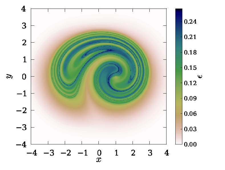
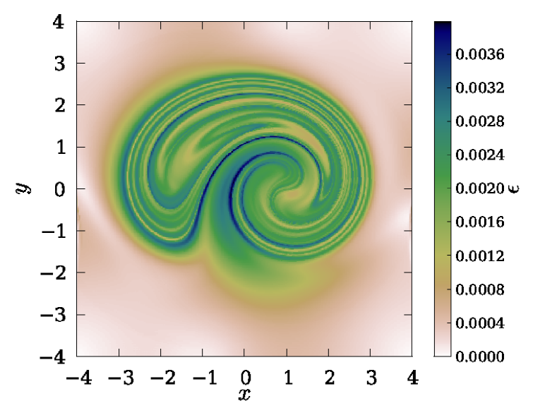
Figure 4.— Average modulus of the Lorentz force along magnetic field lines for the $E^{3}$ configuration with line tied boundaries at $t=0$ (upper panel) and $t=60$ (lower panel).

While $\epsilon$ measures the strength of the forces along the field lines, $\lambda^{*}$ measures the deviation from the force-free state, i.e. $\mbox{\boldmath$\nabla$}{}\times\bm{B}=\alpha\bm{B}$ with $\bm{B}\cdot\mbox{\boldmath$\nabla$}{}\alpha=0$. As expected, the system approaches a state close to force-free (Figure 5). At the same time it develops small-scale features, like $\epsilon$ where $\lambda^{*}$ does not change significantly. Those features are a characteristic of this highly twisted field which were illustrated by e.g. Yeates et al. (2010). From Figure 5 we can conclude that, although the overall system approaches a more force-free state it does so only on average while locally being prevented to reach that state.

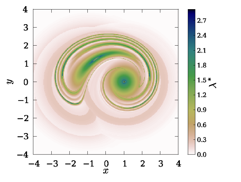
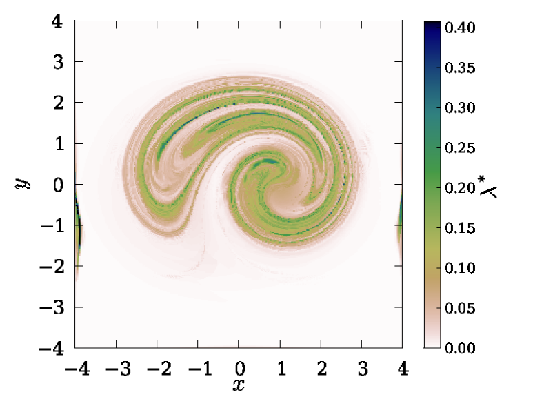
Figure 5.— Maximum gradient of the force-free parameter $\lambda$ along all magnetic field lines for the $E^{3}$ configuration with line tied boundaries $t=0$ (upper panel) and $t=60$ (lower panel).

By using color maps of the magnetic field line Yeates et al. (2010) showed that regions of different field line mappings are connected to a non-trivial topology of the field. Similarly we observe regions where the sign of the twist $\omega$ changes sharply (Figure 6). Those are exactly the loci where both $\epsilon$ and $\lambda^{*}$ develop into thin structures and $\lambda^{*}$ stays approximately constant in time.

The reason that $\epsilon$ and $\lambda^{*}$ develop thin structures as the relaxation proceeds is not clear. This could be a feature of the numerical method employed to perform the relaxation: specifically that under certain conditions the scheme acts to reduce the $\mbox{\boldmath$J$}{}\times\bm{B}$ force on average within the domain at the expense of particular locations at which the relaxation is compromised. On the other hand, it is possible that this is associated with some more fundamental property of the magnetic field. In particular, it could be that the topology of the field, as manifested through the sign change of the average field line twist $\omega$ impedes the further evolution of the field into a perfectly force-free state. In order to determine whether this is the case we require to develop a theory for the evolution of these quantities. This is outside the scope of the present study.

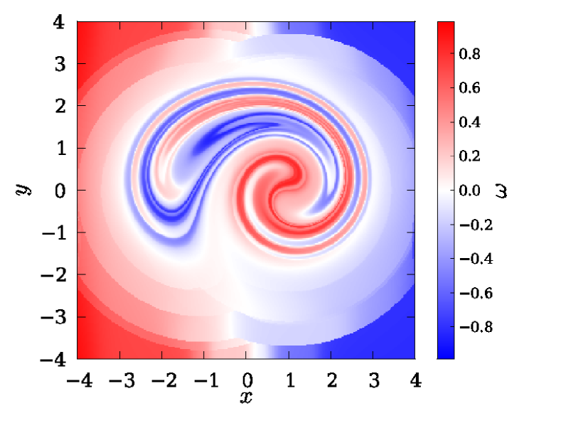
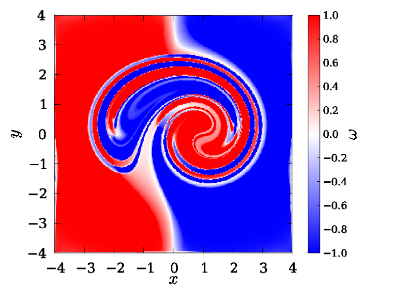
Figure 6.— Average twist of the magnetic field lines $\omega$ for the $E^{3}$ configuration at $t=0$ (upper panel) and $t=60$ (lower panel).

4. Current Formation at Null-Points

With the present framework we are able to investigate the formation of potentially singular current concentrations around magnetic null-points where $\bm{B}=0$. As noted previously there is strong evidence that in response to appropriate perturbations singular current concentrations form at nulls in the perfectly conducting limit (Syrovatskiǐ, 1971; Pontin & Craig, 2005; Fuentes-Fernández & Parnell, 2012, 2013; Craig & Pontin, 2014). Here we embed the null point at the base of a coronal loop. In particular, we take the first twist region of the magnetic field $E^{3}$ considered in the previous section and insert a parasitic polarity flux patch on the lower $z$-boundary, above which is associated a null point within the domain, located at $(-0.2229,-0.2229,-7.08330)$. The separatrix surfaces of this null point forms a dome geometry that encloses the parasitic polarity. The extent of the domain is from $(-4,-4,-8)$ to $(4,4,0)$ (Figure 7).

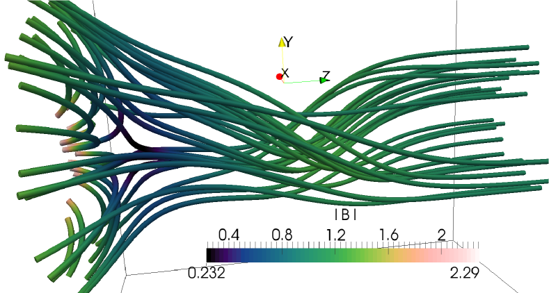
Figure 7.— Initial magnetic field for the configuration with the magnetic dome containing the magnetic null and the first twist region of the $E^{3}$ configuration at the lower boundary at $z=-8$. The colors denote the magnetic field strength.

We study the evolution of this configuration using inertial terms and velocity damping and replace the evolution of the grid positions by using equation (5). Here we set $\nu=3$ and choose a grid resolution of $192^{3}$. This choice of damping term ensures that the magnetic field does not overshoot the equilibrium and instead creeps towards it.

As the field evolves it tries to find a relaxed state of reduced Lorentz force. On average over the domain this does occur. However, in the absence of plasma pressure, near the null point the current density increases to such high values that also the Lorentz force starts to diverge, after which the simulation stops. The loci of these singular current concentrations are at the magnetic nulls, as is highlighted in Figure 8. In line with previous works this current concentration forms as the spine and fan of the null point collapse towards one another (Pontin & Craig, 2005; Fuentes-Fernández & Parnell, 2013). To ensure that this is not a numerical artifact one can check that in the absence of the perturbation – i.e. setting $k=0$ in Equation (17), there is no current growth at the nulls. It should be noted that varying the parameter $\nu$ or resorting to the magneto frictional approach does not qualitatively change this result.

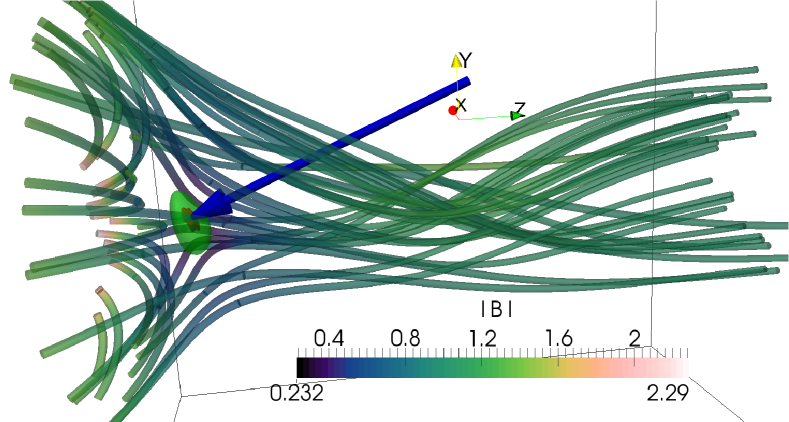
Figure 8.— Final magnetic field for the first twist region of the $E^{3}$ configuration with a magnetic dome together with isosurfaces of the magnetic field (green, half transparent) and current density (red opaque). For the magnetic field we choose a level for the isosurface close to $0$ to highlight the area around the null, while for $J$ we choose a high value. It can be seen that the high current concentration lies at the magnetic null.

Adding a pressure term to our calculations the collapse of the fluid at the magnetic nulls is halted before the numerical instability sets in. To achieve this we replace equation (5) by (6) for the evolution of the fluid and vary the parameter $\beta$ which represents the relative weight of the pressure gradient to the Lorentz force. Even with the pressure gradient present we expect singular current concentrations to form since in general the Lorentz force associated with the null point collapse is not irrotational, and therefore cannot be balanced by the pressure gradient (Parnell et al., 1997; Craig & Litvinenko, 2005; Pontin & Craig, 2005). Indeed, this is what we observe in our simulations where we monitor the maximum current $|J|_{\rm max}$ in the domain at the stage of hydrostatic equilibrium (Figure 9). By decreasing $\beta$ the maximum current increases, as the system gets closer to the zero $\beta$ case. Increasing the grid resolution we observe a systematic increase of $|J|_{\rm max}$, suggesting that we are dealing with a physical current singularity similar to simulations for kink instability by Ali & Sneyd (2001). This holds also true for the case where we replace the magneto-frictional term by equation (5). As noted by Craig & Litvinenko (2005); Pontin & Craig (2005), the effect of the plasma pressure is to weaken the divergent scaling of the peak current density with resolution, indicating that for large values of $\beta$ a weaker singularity is present.

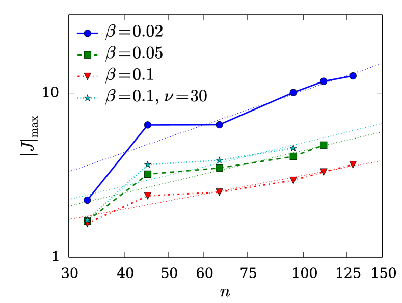
Figure 9.— Maximum current $|J|_{\rm max}$ at hydrostatic equilibrium for different grid resolutions and pressure parameters $\beta$ for the configuration with the magnetic null. The increase with resolution suggests the existence of a singular current concentration.

5. Sheared Fields

Past simulations by Longbottom et al. (1998) of sheared magnetic fields suggested the occurrence of singular current sheets in the absence of magnetic nulls for sufficiently large shear perturbations. Such fields would then not reach a smooth force-free equilibrium supporting the conjecture of Parker (1972). As evidence they pointed to an increasing maximum current density as they increased the numerical resolution and concluded that the increase will continue indefinitely. As maximum resolution they were able to use $65^{3}$ grid points.

Here we propose that their maximum resolution was too low to make any meaningful conclusions about the formation of singular current sheets for cases in which the field is highly sheared. As remedy we perform simulations with high resolutions and monitor the formation of current layers. The field configurations are identical to the ones used by Longbottom et al. (1998). A Cartesian box of size 2 in each dimension is filled with a homogeneous magnetic field in $z$-direction. Subsequently the box is distorted in the $y$-direction according to

$$y=y_{0}-S_{A}\sin{(2\pi S_{K}(x_{0}+O_{x})/L_{x})}z,$$ (18)

after which we apply a distortion in the $x$-direction:

$$x=x_{0}-S_{B}\sin{(2\pi S_{K}(y+O_{y})/L_{y})}z.$$ (19)

Here $x_{0}$ and $y_{0}$ are the grid coordinates of the undistorted Cartesian grid, $S_{A}$ and $S_{B}$ the shearing strengths, $S_{K}$ the wave number, $O_{x}$ and $O_{y}$ the origins of the coordinate system in $x$ and $y$ and $L_{x}$ and $L_{y}$ the length of the box in $x$ and $y$. Here we set the size of the undistorted box to $L_{x}=L_{y}=L_{z}=2$ and center the domain at the origin. We choose $S_{A}=S_{K}=1$ in all the runs and vary $S_{B}$ between $0.1$ and $1$. Note that the distortion in $x$-direction is performed after the one in $y$-direction which is why we use $y$ instead of $y_{0}$ in Equation (19). For the $z$-boundaries we apply the line tied condition where the normal component of the field is fixed and the grid is rigid. The $x$ and $y$ boundaries are periodic. An example initial configuration is shown in Figure 10 for $S_{B}=1$.

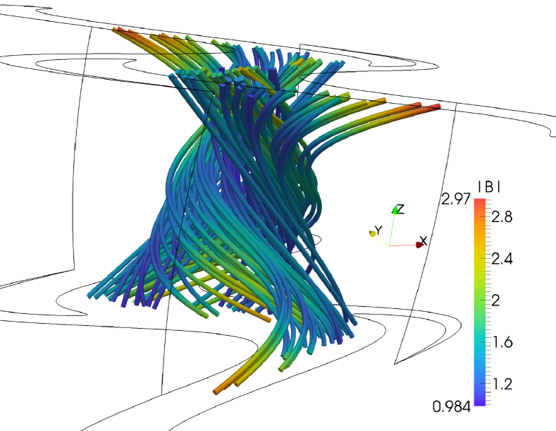
Figure 10.— Initial magnetic field for the sheared field configuration with $S_{B}=1$ together with the distorted grid box.

As the field relaxes towards a more force-free state, the maximum current in the simulation domain increases, forming a thin layer running up the center of the domain, centered on the $z$-axis – see Figure 11. After some time, however, the growth of the peak current in the domain flattens off and a stable spatio-temporal maximum $|J|_{\rm max}$ is attained. Plotting this global maximum of the current as a function of the grid resolution for large shears we observe an increase with resolution (Figure 12), that eventually saturates – further increase of the gird resolution does not lead to an increased current, indicating that an underlying finite current layer has been resolved. This saturation value strongly increases with shearing parameter $S_{B}$, as the field distortion produces strong currents. Figure 13 shows that this increase is exponential. This is in line with recent findings by Pontin & Hornig (2015) who found an exponential increase in the maximum current with increasing twist parameter for the $E^{3}$ field. Furthermore, we do not observe any hint for a threshold after which the field shows current singularities in accordance with Parker’s hypothesis. Already our field with $S_{B}=1$ is so strongly twisted that Parker would have predicted such singularities.

The reason why Longbottom et al. (1998) drew the premature conclusion that singular current sheets for $S_{B}>0.4$ were present was simply due to their limited maximum resolution, which suggested that above a certain $S_{B}$ $|J|_{\rm max}$ would grow indefinitely with the resolution suggesting the formation of singular current sheets. What is clear is that for the grid resolutions they considered an unresolved current concentration below the grid scale was present. However, with our high resolution simulations we are able to resolve the current concentrations even for high grid distortions (Figure 11).

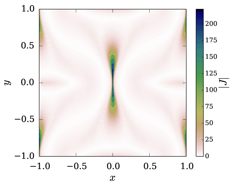
Figure 11.— Map of the current density for the sheared field numerical experiments for $S_{B}=1$ at $z=0$ and final time. Although the current concentrates in a small location it is still resolved with the $180^{3}$ grid points used here and compressed grid cells at high current concentrations.

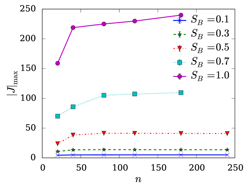
Figure 12.— Maximum current density $|J|_{\rm max}$ in the saturated state in dependence of the grid resolution $n$ for various shearing parameters $S_{B}$ for the sheared field configurations. For all $S_{B}$ there is eventually a flattening off of the curves.

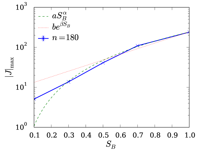
Figure 13.— Maximum current density $|J|_{\rm max}$ in the saturated state in dependence of the shear parameter $S_{B}$ for the resolution $n=180$ for the sheared field configurations together with a power law and exponential fit. Apart from the case with $S_{B}=1$ all the values perfectly align with an exponential law better than with a power law. For the fit parameters we use a least square method and find $a=240.95$, $\alpha=2.35$, $b=9.6057$, $\beta=3.232$.

6. Conclusions

We have introduced a new computational code (Candelaresi, 2015) that performs an exactly ideal relaxation towards an equilibrium magnetic field. This was used to study the properties of equilibria of various magnetic topologies. Several implementations of the relaxation procedure were discussed. We implemented both a magneto-frictional approach and an approach with velocity damping including plasma inertia. In both cases a relaxation towards a force-free state or a magnetohydrostatic equilibrium with finite pressure were discussed. The code uses a Lagrangian grid approach, and in contrast to previous implementations employs mimetic derivatives that lead to an improved approximation of the final equilibrium (Candelaresi et al., 2014).

We have investigated the ideal evolution of topologically non-trivial magnetic field configurations and monitored the behavior of the electric current density. The emphasis was on determining whether singular current sheets might form for fields which are sufficiently stressed, as suggested by Parker (1972). Contrary to Parker’s hypothesis we do not find singular current sheets and all current structures remain resolved in the absence of magnetic nulls.

The first type of field considered was a braided field that has been previously well studied. In support of the previous results (e.g. Wilmot-Smith et al., 2009) we find only well resolved current structures. However, we have noted that at contact areas between regions with different field line twist, the relaxation of the field towards the force-free state is inhibited, as measured by various field line integrated quantities. This suggests that at least using the artificial path to equilibrium discussed here, there may be a barrier to reaching the lowest energy state. This will be discussed further in a future publication. One should note that, as argued by Pontin & Hornig (2015), for braided fields of this nature that exhibit a field line mapping with very small length scales, any equilibrium that does exist must exhibit current layers on these same small length scales. Thus, while Parker’s hypothesis for spontaneous formation of current singularities may not hold for these fields, the proposal that magnetic braiding can provide a source of coronal heating is still valid. In particular, as the field is continually braided by the turbulent convective motions, the length scales of the current layers will eventually become sufficiently small that reconnection occurs.

We also considered sheared magnetic fields that had previously been implicated in the formation of current singularities. We demonstrated that with sufficient grid resolution, a finite current layer can always be resolved, in contradiction to the results of Longbottom et al. (1998), who were severely limited in the grid resolution available to them.

Lastly, we have considered magnetic fields containing magnetic nulls. We showed that in their presence, strong and unresolved current structures form at their loci. This has been previously observed in various studies (Pontin & Craig, 2005; Fuentes-Fernández & Parnell, 2012, 2013; Craig & Pontin, 2014). In most of these previous studies a simple linear null point was considered. Here we considered a coronal loop with a null point near the line-tied boundary in a separatrix dome configuration – the perturbation to the field was applied far form the null point. Nonetheless, the null point still attracted an intense current.

References

- Ali & Sneyd (2001) Ali, F., & Sneyd, A. 2001, Geophysical & Astrophysical Fluid Dynamics, 94, 221
- Batchelor (1950) Batchelor, G. K. 1950, Royal Society of London Proceedings Series A, 201, 405
- Berger (1986) Berger, M. A. 1986, Geophysical & Astrophysical Fluid Dynamics, 34, 265
- Candelaresi (2015) Candelaresi, S. 2015, GLEMuR, https://github.com/SimonCan/glemur
- Candelaresi et al. (2014) Candelaresi, S., Pontin, D., & Hornig, G. 2014, SIAM Journal on Scientific Computing, 36, B952
- Chodura & Schlüter (1981) Chodura, R., & Schlüter, A. 1981, J. Comput. Phys., 41, 68
- Craig & Litvinenko (2005) Craig, I., & Litvinenko, Y. 2005, Phys Plasmas, 12, 032301
- Craig & Sneyd (2005) Craig, I., & Sneyd, A. 2005, Solar Physics, 232, 41
- Craig & Pontin (2014) Craig, I. J. D., & Pontin, D. I. 2014, ApJ, 788, 177
- Craig & Sneyd (1986) Craig, I. J. D., & Sneyd, A. D. 1986, ApJ, 311, 451
- Fuentes-Fernández & Parnell (2012) Fuentes-Fernández, J., & Parnell, C. E. 2012, Astron. Astrophys., 544, A77
- Fuentes-Fernández & Parnell (2013) —. 2013, Astron. Astrophys., 554, A145
- Hyman & Shashkov (1997) Hyman, J. M., & Shashkov, M. 1997, Comput. Math. Appl., 33, 81
- Longbottom et al. (1998) Longbottom, A. W., Rickard, G. J., Craig, I. J. D., & Sneyd, A. D. 1998, ApJ, 500, 471
- Longcope & Strauss (1994) Longcope, D. W., & Strauss, H. R. 1994, ApJ, 437, 851
- Low (2010) Low, B. 2010, Solar Physics, 266, 277
- Low (2013) Low, B. C. 2013, ApJ, 768, 7
- Mikic et al. (1989) Mikic, Z., Schnack, D. D., & van Hoven, G. 1989, ApJ, 338, 1148
- Parker (1972) Parker, E. N. 1972, ApJ, 174, 499
- Parker (1983a) —. 1983a, ApJ, 264, 642
- Parker (1983b) —. 1983b, ApJ, 264, 635
- Parnell et al. (1997) Parnell, C. E., Neukirch, T., Smith, J. M., & Priest, E. R. 1997, Geophysical and Astrophysical Fluid Dynamics, 84, 245
- Pontin & Craig (2005) Pontin, D. I., & Craig, I. J. D. 2005, Phys. Plasmas, 12, 072112
- Pontin & Hornig (2015) Pontin, D. I., & Hornig, G. 2015, ApJ, 805, 47
- Pontin et al. (2009) Pontin, D. I., Hornig, G., Wilmot-Smith, A. L., & Craig, I. J. D. 2009, ApJ, 700, 1449
- Priest & Forbes (2000) Priest, E. R., & Forbes, T. G. 2000, Magnetic reconnection: MHD theory and applications, ed. C. U. Press
- Syrovatskiǐ (1971) Syrovatskiǐ, S. I. 1971, Soviet Journal of Experimental and Theoretical Physics, 33, 933
- van Ballegooijen (1985) van Ballegooijen, A. A. 1985, ApJ, 298, 421
- van Ballegooijen (1988) —. 1988, Geophys. Astrophys. Fluid Dynamics, 41, 181
- Wilmot-Smith et al. (2009) Wilmot-Smith, A. L., Hornig, G., & Pontin, D. I. 2009, ApJ, 696, 1339
- Wilmot-Smith et al. (2010) Wilmot-Smith, A. L., Pontin, D. I., & Hornig, G. 2010, A&A, 516, A5
- Yang et al. (1986) Yang, W. H., Sturrock, P. A., & Antiochos, S. K. 1986, ApJ, 309, 383
- Yeates et al. (2010) Yeates, A. R., Hornig, G., & Wilmot-Smith, A. L. 2010, Phys. Rev. Lett., 105, 085002