Duality between Temporal Networks and Signals: Extraction of the Temporal Network Structures

Abstract

We develop a framework to track the structure of temporal networks with a signal processing approach. The method is based on the duality between networks and signals using a multidimensional scaling technique. This enables a study of the network structure using frequency patterns of the corresponding signals. An extension is proposed for temporal networks, thereby enabling a tracking of the network structure over time. A method to automatically extract the most significant frequency patterns and their activation coefficients over time is then introduced, using nonnegative matrix factorization of the temporal spectra. The framework, inspired by audio decomposition, allows transforming back these frequency patterns into networks, to highlight the evolution of the underlying structure of the network over time. The effectiveness of the method is first evidenced on a toy example, prior being used to study a temporal network of face-to-face contacts. The extraction of sub-networks highlights significant structures decomposed on time intervals.

1 Introduction

Many complex systems, whether physical, biological or social, can be naturally represented as networks, i.e., a set of relationships between entities. Network science [28] has been widely developed to study such objects, generally supported by a graph structure, by providing powerful tools, such as the detection of communities [12], in order to understand the underlying properties of these systems. Recently, connections between signal processing and network theory have emerged: The field of signal processing over networks [31, 29] has been introduced with the objective of transposing concepts developed in classical signal processing, such as Fourier transform or wavelets, in the graph domain. These works have led to significant results, among them filtering of signals defined over a network [31] or multiscale community mining using graph wavelets [33]. These approaches benefit from the natural representation of networks by graphs, enabling the use of the comprehensive mathematical understanding of graph theory. Another approach has been also considered, defining a duality between graphs and signals: methods have been developed to transform graphs into signals and conversely, in order to take advantage of both signal processing and graph theory. Hence, mapping a graph into time series has been performed using random walks [34, 3, 15] or deterministic methods based on classical multidimensional scaling [23, 30]. This latter approach has been the topic of several extensions in [22], in order to build a comprehensive framework to link frequency patterns of the so-obtained signals with network structures.

Studies mainly focused on the analysis of static networks, potentially aggregated over time, but without time evolution. However, the considered systems are most of the time not frozen: vertices and edges appear and disappear over the course of time. Aggregating the networks over a time interval gives insight of the underlying mechanisms, but often does not provide the actual dynamic sequence of appearance and disappearance of edges: two edges, active one after the other, will be considered simultaneous in the temporally-aggregated network. Given the importance of knowing such dynamics, for instance in topics such as epidemic spread or communication networks, and thanks to the recent availability of many data sets, a temporal network theory has recently appeared [24, 4], enabling a deeper understanding of underlying mechanisms. Several studies proposed an extension of the methods developed for static networks to the temporal case: we can cite for instance works on network modeling [2, 7, 16, 35], detection of communities [27, 37, 14, 13, 5], detection of temporal motifs [25], visualization [36], or more generally data mining of time-evolving sequences [38].

We propose in this article a new approach based on the duality between networks and signals to study temporal networks, introduced in [22]. The objective here is to follow the global structure of the network over time. One first contribution consists of an extension of the existing work to the temporal case, which is naturally performed by considering each time instant as a static network. This approach enables us to visually track temporal networks by following the frequency patterns associated to specific structures. The second contribution consists of using nonnegative matrix factorization (NMF) [26] to automatically extract and track the significant frequency patterns over time. Details about the reconstruction how components can be transformed back into networks are also provided.

Preliminary versions of this work have been presented in different places: the principle of extension of the method to the temporal case is introduced in [19], as well as the visual tracking of frequency patterns representing structures. In [18, 17], this approach has been used to study a bike sharing system in Lyon, which is not mentioned in this article. Finally, the idea of the decomposition using NMF has been suggested in [20]. This paper extends however those previous works by detailing a comprehensive framework and setting out consistent arguments for the validity of the method in the context of analysis of temporal networks.

The paper is organized as follows. Section 2 recalls the duality between static networks and signals, as introduced in [30] and extended in [22]. Section 3 gives an extension of the transformation to the temporal case, and introduces a toy temporal network highlighting specific network structures. Section 4 shows how spectral analysis is used to track the structure of the temporal network over time, while Section 5 describes a decomposition of a temporal network into sub-networks by applying nonnegative matrix factorization to the matrix of spectra over time. For both sections, an illustration with the toy temporal network is provided. Finally, Section 6 applies the developed framework to a real-world temporal network from the SocioPatterns project, describing face-to-face contact between children in a primary school.

Notations

Matrices are denoted by boldface capital letters, their columns by boldface lowercase letters, and their elements by lowercase letters: for $\bm{M}\in\mathbb{R}^{A\times B}$, $\bm{M}=[\bm{m}_{1},\ldots,\bm{m}_{B}]=(m_{ab})_{a\in\{1,\ldots,A\},b\in\{1,\ldots,B\}}$. Tensors are represented by calligraphic capital letters: for $\mathcal{T}\in\mathbb{R}^{A\times B\times T}$, $\mathcal{T}=[\bm{M}^{(t)}]_{t\in\{1,\ldots,T\}}$. Operators are represented by calligraphic boldface capital letters: $\bm{\mathcal{F}}$.

2 Duality between static networks and signals

2.1 Transformation from static networks to signals

Duality between networks and signals has been introduced to analyze networks structures using signal processing tools. Shimada et al. [30] proposed a method to transform static networks into a collection of signals using multidimensional scaling. We proposed in [22] a comprehensive framework to transform graphs into a collection of signals, based on this work. We recall in this section the main principles of this framework, which will be used in the following to study temporal networks. We consider in the following networks described by unweighted and undirected graph with $N$ vertices.

In [30], Classical MultiDimensional Scaling (CMDS) [1] is used to transform a graph into signals by projecting the $N$ vertices of the graph in a Euclidean space, such that distances between these points correspond to relations in the graph. The graph is fully described by its adjacency matrix $\bm{A}\in\mathbb{R}^{N\times N}$, whose elements $a_{ij}$ are equal to $1$ if vertices $i$ and $j$ are linked, and $0$ otherwise. The transformation consists in applying CMDS to a matrix encoding distance between vertices of a graph, noted $\mathbf{\Delta}=(\delta_{ij})_{i,j=1,..,N}$, and defined for two vertices $i,j$ of the network by:

$$\delta_{ij}=\left\{\begin{array}[]{l l}0&\quad\text{if $i=j$}\\ 1&\quad\text{if $a_{ij}=1$ and $i\neq j$}\\ w>1&\quad\text{if $a_{ij}=0$ and $i\neq j$}\\ \end{array}\right.$$ (4)

As discussed in [22], we choose $w=1+\frac{1}{N}$. This definition focuses on the presence (denoted by a distance equal to $1$) or the absence (denoted by a distance equal to $w$) of an edge between two vertices. Hence, the distance of two vertices in the graph, often defined as the length of the shortest path between the two vertices, has no direct impact on the matrix $\bm{\Delta}$: two pairs of unlinked vertices will have a distance equal to $w$, whether they are close or not in the graph. Applying CMDS on the distance matrix $\bm{\Delta}$ leads to a collection of points, corresponding to the vertices, in a Euclidean space $\mathbb{R}^{N-1}$. The considered signals, or components, correspond to the coordinates, for each dimension, of the points. The collection of signals is denoted by $\bm{X}\in\mathbb{R}^{N\times C}$, where $C$ is the total number of components, and thus is equal to $N-1$ for the full representation. The columns $\bm{x}_{c}$ represent the $c$-th signal, with $c\in\{1,\ldots C\}$, and are indexed by the vertices. The transformation is denoted by $\bm{\mathcal{T}}$: $\bm{\mathcal{T}}[\bm{A}]=\bm{X}$.

2.2 Inverse Transformation

Transforming back signals to a graph has to take into account the nature of the signals, as they are a representation of a specific network. The inverse transformation must hence preserve the original topology of the underlying graph. By construction of the collection of signals $\bm{X}$, the perfect retrieval of the underlying graph is easily reachable, by considering the distances between each pair of point: As built using CMDS, these distances represent the distance matrix $\bm{\Delta}$, and the adjacency matrix of the graph is directly obtained. However, when $\bm{X}$ is degraded or modified, e.g. by taking $C<N-1$, the distances are no longer directly the ones computed between vertices, even if they stay in the neighborhood of these distances. We proposed in [22] to take into account the energy of components to improve the reconstruction, as well as prior information about the original graph. If the distance between two vertices $i$ and $j$ in a high-energy component is high, it means that the two vertices are likely to be distant in the graph. Conversely, if the distance in a high-energy component is low, then the two vertices are likely to be connected in the graph.

Let $\tilde{\bm{X}}$ be a degraded collection of signals. The energies are normalized according to the energies of the original components, by multiplying the components $\tilde{\bm{x}}_{c}$ by the normalization factor $N_{c}$:

$$N_{c}=\sqrt{\frac{\sum_{n=1}^{N}x_{nc}^{2}}{\sum_{n=1}^{N}\tilde{x}_{nc}^{2}}}$$ (5)

Then the distances are computed by using the energies as follows:

$$d(\bm{X})_{ij}=\sqrt{\sum_{c=1}^{C}{(u_{c})^{\alpha}(x_{ic}-x_{jc})^{2}}}$$ (6)

with $\alpha\geq 0$, where $u_{c}$ is the energy of component $c$, computed as $u_{c}=\sum_{i=1}^{n}{x_{ic}^{2}}$, and normalized such that $\|\bm{u}\|_{\alpha}=\sum_{c=1}^{C}(u_{c})^{\alpha}=C$, with $\bm{u}$ the vector of energies for all components. The parameter $\alpha$ controls the importance of the weighting: if $\alpha$ is high, the high-energy components have a higher importance in the computation of distances compared to the low-energy components. Conversely, if $\alpha$ is small, the importance of high-energy components is diminished. In particular, $\alpha=0$ gives the standard reconstruction. The distances are then thresholded, by retaining the edges corresponding to the smallest distances. The threshold is chosen in order to recover the same amount of edges than in the original network. This inverse transformation is denoted $\bm{\mathcal{T}^{-1}}$: $\bm{\mathcal{T}^{-1}}[X]=\bm{A}^{(r)}$, where $\bm{A}^{(r)}$ is the adjacency matrix of the reconstructed graph.

2.3 Indexation of signals

As the signals are indexed by the vertices, the order in which we consider them in the transformation is essential to study some aspects of the signals, especially when using spectral analysis of the signals. Ordering randomly the vertices does not change the value assigned to each vertex, but would lead to abrupt variations in the representation of signals: Specific frequency properties, clearly observable in signals, will no longer be visible. Unfortunately, the suitable ordering is usually not available, especially when dealing with real-world graphs. To address this issue, we proposed in [21] to find a vertex ordering that reflects the topology of the underlying graph, based on the following assumption: if two vertices are close in the graph (by considering for instance the length of the shortest path between them), they have to be also close in the ordering. Details of the algorithm and results about the consistency between the obtained vertex ordering and the topology of the graph are covered in [21].

2.4 Spectral analysis of signals

Spectral analysis is performed using standard signal processing methods: Let a collection $\bm{X}$ of $C$ signals indexed by $N$ vertices. The spectra $\bm{S}\in\mathbb{R}^{C\times F}$ give the complex Fourier coefficients, whose elements are obtained by applying the Fourier transform on each of the $C$ components of $\bm{X}$:

$$\bm{s}_{c}=\bm{\mathcal{F}}[\bm{x}_{c}]$$ (7)

estimated, for positive frequencies, on $F=\frac{N}{2}+1$ bins, $\bm{\mathcal{F}}$ being the Fourier transform and $c\in\{1,\ldots,C\}$.

From the spectrum $\bm{S}$, the following features are obtained for each frequency of each component:

• the magnitudes $\bm{M}$, which read as $m_{cf}=|s_{cf}|$

• the energies $\bm{E}$, which read as $e_{cf}=|s_{cf}|^{2}$

• the phases $\bm{\Phi}$, which read as $\phi_{cf}=\arg(s_{cf})$

The matrices $\bm{M}$ and $\bm{E}$ are studied as a frequency-component map, exhibiting patterns in direct relation with the topology of the underlying graph. The phases of signals $\bm{\Phi}$ are used in the inverse Fourier transformation, when the collection of signals has to be retrieved from $\bm{M}$ or $\bm{E}$.

2.5 Illustrations

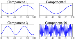
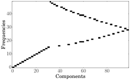
(a) $4$-ring lattice

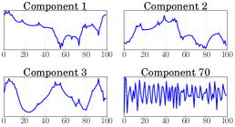
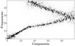
(b) Noised $4$-ring lattice with $p=0.1$

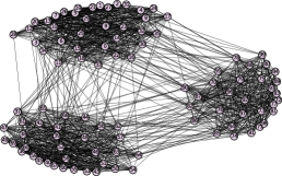
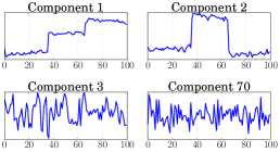
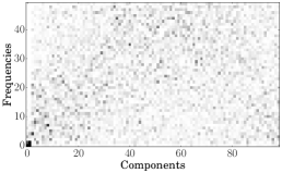
(c) Stochastic block model with $3$ communities, $p_{w}=0.8$ and $p_{b}=0.05$

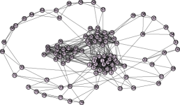
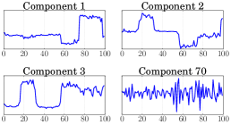
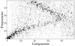
(d) $4$-ring lattice with $3$ communities

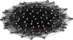
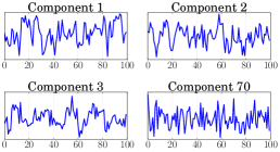
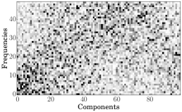
(e) Erdös-Rényi model with $p=0.4$

Figure 1: Illustrations on several instances of network models of the transformation of a network into a collection of signals. All networks have $N=100$ vertices. (Left) Two-dimensional representation of the network. (Middle) First three highest energy components, and the arbitrarily chosen component $70$, a low-energy one. (Right) Component-frequency map obtained after spectral analysis. The color represents the intensity, coded from white to black. The contrast is emphasized to expose the patterns.

Figure 1 shows illustrations of the transformation of a graph into a collection of signals, on several instances of network models. These illustrations show the connection between graph structure and the resulting signals after transformation. Regular structures (Figures 1a and 1b) highlight harmonic oscillations as components, while an organization in communities (Figure 1c) presents high-energy frequencies on the first components. Combination of both structures in the graph (Figure 1d) is preserved in the frequency pattern. Finally, a random graph (Figure 1e) leads to a similar absence of structure in the corresponding frequency pattern.

3 Extension to temporal networks

3.1 Transformation of temporal networks into signals and back

The description of temporal networks considered in this work consist in a discrete-time sequence of graph snapshots. The collection of all snapshots at the different times $t\in\{0,\ldots,T-1\}$, with $T$ the total number of time steps, can be represented by a graph adjacency tensor denoted $\mathcal{A}\in\mathbb{R}^{N\times N\times T}$. We study here temporal networks where the edges are changing over time, keeping the same given set of vertices (possibly isolated).

The extension of the method described in Section 2 is directly achieved by applying at each time step the transformation on the corresponding static representation of the temporal network. We denote $\mathcal{X}\in\mathbb{R}^{N\times C\times T}$, the collection of signals obtained from $\mathcal{A}$. For each time step $t$, we have

$$\bm{X}^{(t)}=\bm{\mathcal{T}}[\bm{A}^{(t)}]$$ (8)

As the number of vertices in the graph does not evolve, the number of components $C$, and then the number of frequencies $F$, is constant over time. In the case where the set of vertices evolves, the tensor is built by fixing the number of components as the maximal number of components over time, and by zero-padding the missing components. As for the indexation of vertices, the algorithm relabeling vertices according to the structure of the network is performed at each time step, leading to a different labeling of the vertices over time.

Conversely, the inverse transformation is performed likewise, by applying the static inverse transformation on the collection of signals at time $t$:

$$\bm{A}^{(t,r)}=\bm{\mathcal{T}^{-1}}[\bm{X}^{(t)}]$$ (9)

where $\bm{A}^{(t,r)}$ represents the adjacency matrix of the reconstructed temporal network at time $t$.

3.2 Illustration on a Toy Temporal Network (TTN)

Table 1: Generation of the Toy Temporal Network: Probabilities to have an edge at time $t$

	$e\in E^{p}$	$e\notin E^{p}$
$e\in E_{t-1}$	$0.99$	$0.8$
$e\notin E_{t-1}$	$0.2$	$0.01$

A toy temporal network is introduced for the sake of illustration. The temporal network consists of smooth transitions between different network structures. Starting from $N$ unconnected vertices, the algorithm adds or removes edges at each time instant according to a probability depending both on the presence or not of the edge at the previous time, and on a prescribed network structure. Let $E_{t}$ be the set of edges at time $t$, $E^{p}$ the set of edges of a prescribed network structure, and $e=(i,j)$ the edge between the vertices $i$ and $j$. Table 1 gives the probability to have $e$ in $\mathcal{E}_{t}$ according to the presence of $e$ at the previous time (i.e. $e\in E_{t-1}$) and the presence of $e$ in the prescribed network structure ($e\in E^{p}$). These probabilities are set up in order to generate a smooth transition between the initial structure and the prescribed network structure, and such that the structure at the end of the time interval is close to the one of the prescribed graph.

Four networks are successively chosen as prescribed network structures, among those introduced in Section 2, each structure being active for a time interval of 20 time steps:

1. Random linkage of vertices (see Figure 1e)

2. Network with $3$ communities (see Figure 1c)

3. 4-ring lattice (see Figure 1a)

4. 4-ring lattice with $3$ communities (see Figure 1d)

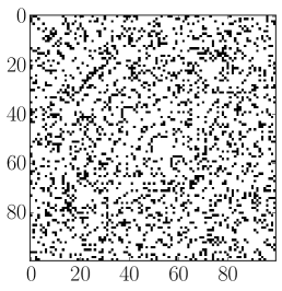
(a) $t=19$

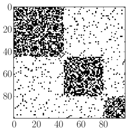
(b) $t=39$

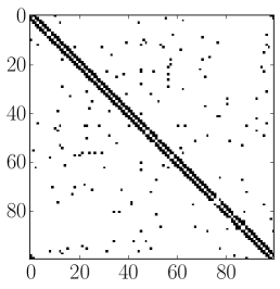
(c) $t=59$

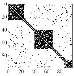
(d) $t=79$

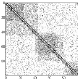
(e) Agg. adjacency matrix

Figure 2: Adjacency matrix $\bm{A}_{t}$ of the Toy Temporal Network at different time instant.

Figure 2 shows the adjacency matrix of the temporal network at the end of each time interval. The prescribed structure is clearly visible thanks to a proper labeling of vertices: the blocks describe the communities, while the strong diagonal describes the regular lattice. These structures are nevertheless not completely defined, as noise due to the probabilities set in Table 1 remains present. It allows to assess the robustness of the further analyses to noise. Figure 2e shows the adjacency matrix of the temporal network aggregated over the $80$ time steps: the four structures also appear using this representation.

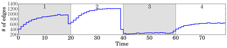
(a) Number of edges

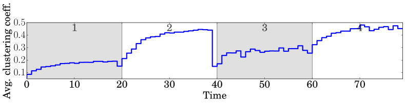
(b) Average clustering coefficient

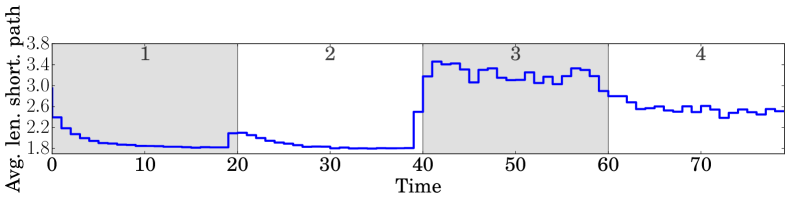
(c) Average length of shortest paths

Figure 3: Descriptors of the Toy Temporal Network over time. The alternating shaded regions correspond to the four different periods, whose the label is given at the top of each region.

Figure 3 plots three descriptors of the network at each time step, which would be a manner to analyze the temporal network using network theory. The number of edges (Figure 3a), the average clustering coefficient (Figure 3b) and the average length of shortest paths (Figure 3c) allow for an identification of the four time intervals: The number of edges increases in the period $2$, to form the random structure, characterized by a low average clustering coefficient and low average length of shortest paths. Adding communities in period $2$ increases the average clustering coefficient, as expected. On the contrary, the regular structure in period $3$ decreases the clustering coefficient and increases the average length of shortest paths, but much less in proportion than the decrease of the number of edges would affect. As expected, adding communities in this regular structure, as it is done in period $4$, significantly increases the average clustering coefficient and slightly decreases the average length of shortest paths. These network-based descriptors give good intuitions on the underlying structure of the temporal network, but turn out to be inefficient to exactly characterize the structure. Furthermore, mixture of different structures, as it appears in this model, are not explicitly revealed.

4 Spectral Analysis of Temporal Networks

4.1 Temporal Spectra

As previously, the extension of the spectral analysis of signals representing networks, defined in Section 2.4 is simply achieved by considering independently each time step. We denote by $\mathcal{S}\in\mathbb{R}^{C\times F\times T}$ the spectral tensor, where $\bm{S}^{(t)}$ corresponds to the spectra obtained at time $t$. The corresponding matrices $\mathcal{M}$ and $\mathcal{E}$ are respectively the temporal magnitudes and energies.

As described in Section 2, the spectra are closely related to the network structures. In particular, the importance of high-energy components as well as low frequencies have been highlighted, for instance for the structure in communities. Looking at the marginals of the temporal energies or magnitudes over frequencies and components is hence expected to give hints about the evolution of the structure of the temporal network over time. In the following, we will focus on the marginal of the energies over the components, denoted $\bm{E}_{c}(f)$, and over the frequencies, denoted $\bm{E}_{f}(c)$.

We also propose to use the spectral analysis to compare two network structures by computing the correlation between their spectra at each time step. The idea is to find among a set of parametric graph models the one that best fit the network at each time step. If we denote by $\bm{S}_{m}$ the spectra obtained after transformation of an instance $\mathcal{G}_{m}$ of a prescribed graph model, we can compute a correlation coefficient $\rho^{(t)}$ between $\bm{S}_{m}$ and $\bm{S}^{(t)}$. Generating several instances of the graph model gives us an average value of the correlation coefficient over several repetitions.

4.2 Illustration on the Toy Temporal Network (TTN)

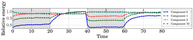
(a) Averaged over frequencies $\bm{E}_{f}(c)$ for $c\in\{0,1,2,70\}$

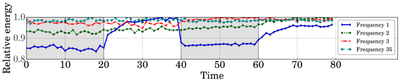
(b) Averaged over components $\bm{E}_{c}(f)$ for $f\in\{1,2,3,35\}$

Figure 4: Marginals of the energies of temporal spectra.

Figure 4 shows $\bm{E}_{c}(f)$ and $\bm{E}_{f}(c)$ for respectively $f\in\{1,2,3,35\}$ and $c\in\{0,1,2,70\}$. These two figures reveal the predominance of the first components and low frequencies, to track an organization in communities of the network: the low frequencies for the first components have a greater energies than for other types of structure, as already remarked in Section 2.5. The tracking of the other types of structures is nevertheless not visible using this representation.

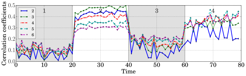
(a) Comparison with a network with $k$ communities, for different values of $k$. The temporal network is highly correlated with a graph organized in communities during the period $2$ and $4$, as expected.

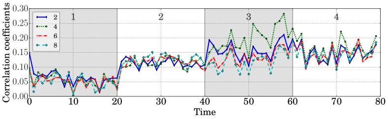
(b) $k$-regular lattice, for different value of $k$. The temporal network has the highest correlation with a $4$-regular lattice during the period $3$.

Figure 5: Correlation between the temporal spectra at each time step and the spectra of networks with two specific network structures. The correlation is averaged over $20$ repetitions.

The correlation between the temporal spectra of the toy temporal network and two network structures is studied. First, a structure in communities is observed, using a network model generating a random graph with a fixed number of communities. The comparison is done for a number of communities from $2$ to $6$, with $20$ repetitions for each number of communities. Figure 5a shows the average correlation: the correlation is maximal during the periods $2$ and $4$, where the network is effectively structured in communities. During the period $2$, the correlation is maximal when the network is structured in $3$ communities, as expected. During the period $4$, the number of communities is not clearly revealed, as the communities are not the only component of the network topology.

In Figure 5b, the temporal network is compared using the same method with a $k$-regular lattice, for $k$ equals to $2$, $4$, $6$ and $8$. If the correlations are lower than previously, we can nevertheless notice that in period $3$, the temporal network is correlated with a $4$-regular lattice, which is the structure set in the prescribed network during this period.

The study of temporal spectra give hence insights about the structure of the underlying temporal network, but this approach is limited by the lack of knowledge, in the general case, of the parametric graph models composing the temporal network. To complement our analysis, we propose in the following to automatically find structures and their corresponding time activation periods that best characterize the temporal network.

5 Extraction of Frequency Patterns using Nonnegative Matrix Factorization

5.1 Nonnegative Matrix Factorization (NMF)

Nonnegative matrix factorization (NMF) [26] is a linear regression technique, used to decompose a nonnegative matrix $\bm{V}$ of dimension $C\times T$, i.e. a matrix whose terms are greater or equal to zero, into the product of two nonnegative matrices $\bm{W}$ and $\bm{H}$. NMF leads to a reduction of the dimensionality of data, by extracting in the columns of $\bm{W}$ patterns characterizing the data, and in the rows of $\bm{H}$ the activation coefficients of each pattern along the time. The number of extracted patterns is denoted $K$. A common approach to achieve such a decomposition consists of solving an optimization problem:

$$(\bm{W}^{*},\bm{H}^{*})=\arg\min_{\bm{W}\bm{H}}D(\bm{V}|\bm{WH})$$ (10)

where $D$ is a dissimilarity measure. Févotte et al. [11] proposed an algorithm to find a solution of the NMF where $D$ is the $\beta$-divergence, a parametric function with a simple parameter $\beta$ which encompasses the Euclidean distance ($\beta=2$), the generalized Kullback-Leibler divergence ($\beta=1$) and the Itakura-Saito divergence ($\beta=0$) as special cases.

Regularization of the activation coefficients can be added in order to smooth them, with the assumption that there is no abrupt variations in the structure from one time step to the next one. The optimization problem is then defined as the minimization of the fitting term, defined in Eq. 10, plus a term of temporal regularization:

$$P(\bm{H})=\sum_{k=1}^{K}\sum_{t=2}^{T}D(h_{k(t-1)}|h_{kt})$$ (11)

leading to:

$$(\bm{W}^{*},\bm{H}^{*})=\arg\min_{\bm{W}\bm{H}}D(\bm{V}|\bm{WH})+\gamma P(\bm{H})$$ (12)

where $\gamma$ controls the regularization and is empirically fixed such that the activation coefficients highlight smoothness. In [9] and [8], smooth NMF has been introduced for $\beta=1$ and $\beta=0$.

5.2 NMF on Spectra of Graphs

Several approaches have been proposed to adapt NMF to networks, either static [39] or temporal [14]. In the latter approach, the adjacency matrix is represented as a tensor and is decomposed using nonnegative tensor factorization (NTF) [6]. The drawback of this approach is that the adjacency matrix at each time step is represented as the product of vectors, which is well-suited to highlight structure in communities but not adapted when the structure becomes more complex.

Following [20], we propose to use NMF to find patterns in spectra of the collections of signals, obtained from the transformation of the temporal network. By analogy with music analysis, where an audio sample is decomposed into several audio samples, separating for instance voice from the instrumental part [10], we would like to decompose the temporal network into temporal sub-networks, decomposing at each time step the global structure into several substructures. Furthermore, audio spectra share similarities with graph spectra. We then propose to use the Itakura-Saito divergence as measure of dissimilarity, given by $d_{IS}(x|y)=\frac{x}{y}-\log\frac{x}{y}-1$. It allows taking advantage of the framework developed to reconstruct the signals from spectra as well as using efficient optimization algorithms with possible temporal regularization.

As the input in our case is the temporal spectra $\mathcal{S}$, represented as a tensor of dimension $C\times F\times T$, a small adaptation has to be performed before applying NMF. At each time instant $t$, the spectra $\bm{S}_{t}$ is represented as a vector $\bm{v}_{t}$ by successively adding end-to-end the columns of the matrix $\bm{S}_{t}$. For all $t\in\{0,\ldots,T-1\}$, these vectors compose the columns of the matrix $\bm{V}$, of dimension $(FC)\times T$. The number of components $K$ is set according to our expectations about the data, and the parameter $\gamma$ is strictly positive to ensure smoothness in the activation coefficients.

5.3 Identification of components

NMF returns two matrices $\bm{W}$ and $\bm{H}$: each column of $\bm{W}$ represents the $k$th (normalized) frequency pattern, while the $k$th column of $\bm{H}^{T}$, gives the activation coefficients of the frequency pattern $k$ at each time step. From $\bm{w}_{k}$, a component-frequency map can be built by reshaping the vector into a matrix. To highlight how these structures are arranged in the temporal network, each component is transformed into temporal network: As described in [10], using NMF with the Itakura-Saito divergence provides means of reconstruction of the collection of signals corresponding to each component. For each component $k$, a temporal spectrum $\mathcal{S}^{(k)}\in\mathbb{R}^{C\times F\times T}$ is obtained using a Wiener filtering such that its elements $s_{cf}^{(k,t)}$ read as:

$$s^{(k,t)}_{cf}=\frac{w_{(cf)k}h_{kt}}{\sum_{l=1}^{K}w_{(cf)l}h_{lt}}s_{cf}$$ (13)

leading to a conservative decomposition of the tensor $\mathcal{S}$:

$$\mathcal{S}=\sum_{k=1}^{K}\mathcal{S}^{(k)}$$ (14)

The temporal spectrum of the component $k$ is then a fraction of the original temporal spectrum. From $\mathcal{S}^{(k)}$, an inverse Fourier transformation is performed, leading to a collection of signals for each component $k$ denoted by $\mathcal{X}^{(k)}\in\mathbb{R}^{N\times N\times T}$. Finally, the adjacency tensor $\mathcal{A}^{(k)}$ describing the temporal network corresponding to the component $k$ is obtained by using the inverse transformation $\bm{\mathcal{T}^{-1}}$ described in Section 3.

5.4 Application to the Toy Temporal Network (TTN)

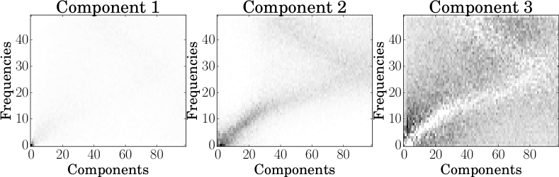
(a) Frequency patterns, obtained after reshaping the columns of $\bm{W}$ into matrices.

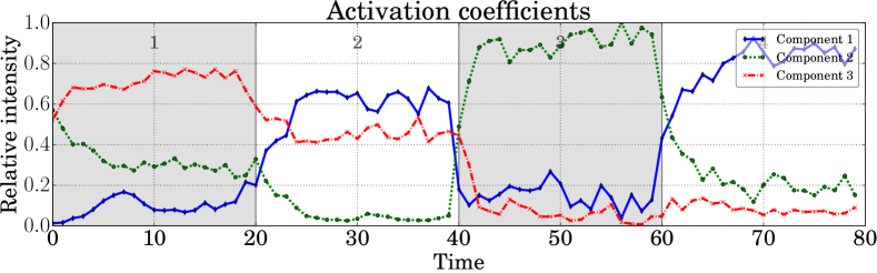
(b) Activation coefficients, corresponding to the rows of the matrix $\bm{H}$, normalized by the maximal value of $\bm{H}$

Figure 6: Results of the nonnegative matrix factorization for the Toy Temporal Network, using $K=3$ and $\gamma=5$.

NMF is applied to the Toy Temporal Network defined in Section 3.2. The matrix $\bm{V}\in\mathbb{R}^{4950\times 80}$ is decomposed using $K=3$ and $\gamma=5$, which is the expected number of structures. Figure 6b shows the activation coefficients of each component. We notice that the activation coefficients are consistent with the division of time introduced in the generation of the temporal network: All components have distinct levels of activation, corresponding to the four different structures used. The component $1$ is active in periods $1$, $2$ and $4$ with an almost constant level, the component $2$ is mainly active in period $3$, as well as in periods $1$ and $4$, and finally, the component $3$ is active in period $1$ and in period $2$.

Looking at the corresponding frequency patterns in Figure 6a, and more precisely their connections with the network structures observed in Section 2.5, confirms the good adequacy with the expected results: The component $1$ looks like a structure in communities, the component $2$ resembles a $k$-regular structure and the component $3$ exhibits random structure. The structure in period $1$ is then a mixture between a random structure and a structure in communities (as it happens, one single community), in period $2$ only the structure in communities is present, in period $3$ a regular structure described by component $2$ and finally, the fourth period is a mixture between structure in communities and regular structure. Random structure is present in period $1$ and in period $2$ inside communities.

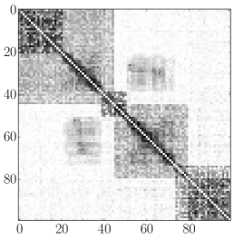
(a) Component 1

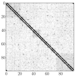
(b) Component 2

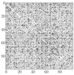
(c) Component 3

Figure 7: Adjacency tensor aggregated over time: for each component $k$, $\bm{A}^{(k)}=\sum_{t=1}^{T}h_{kt}\bm{A}^{(k,t)}$.

Figure 7 shows, for each component $k$, the aggregated adjacency matrix over time, obtained after the back transformation of the spectra into a temporal network. The sum is weighted by the activation coefficients given by the matrix $\bm{H}$, in order to highlight visually the most significant patterns:

$$\bm{A}^{(k)}=\sum_{t=1}^{T}h_{kt}\bm{A}^{(k,t)}$$ (15)

This representation partly confirms the connections between spectra and structures as described above. We can notice that component $1$ displays the three communities present in period $2$, as well as communities corresponding to a regular structure in period $4$. The actual communities in period $4$ are caught in the component $2$, which does not correspond to a regular structure, even if the diagonal, characterizing the $k$-regular lattice, is clearly dominant. Finally, the component $3$ looks like a random matrix, as no structure is visible, at least through this representation.

The decomposition of temporal networks using NMF enables to retrieve from the spectra the different structures composing the temporal network, and to detect when these structures are present, either alone or jointly. We now propose to apply this framework to study a real-world temporal network describing contacts between individuals in a primary school.

6 Temporal Network of Social Interactions Between Children in a Primary School

6.1 Description of the temporal network

The decomposition is applied to a real-world temporal network, describing social interactions between children in a primary school during two days in October 2009. During a 20-second interval, an edge exists between two individuals if a contact is recorded, measured by wearable RFID (Radio Frequency IDentification) sensors [32]. For our study, the data set is described by a temporal network, representing for each time step the aggregated contacts between individuals for 10 minutes. We restrained the analysis to the first day: 226 children and 10 teachers participated in the experiment, separated in five grades (from 1st grade to 5th grade), themselves separated in two classes.

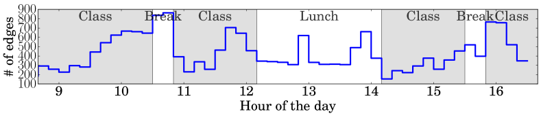
(a) Number of edges

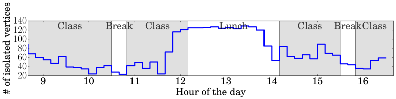
(b) Number of isolated vertices

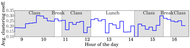
(c) Average clustering coefficient

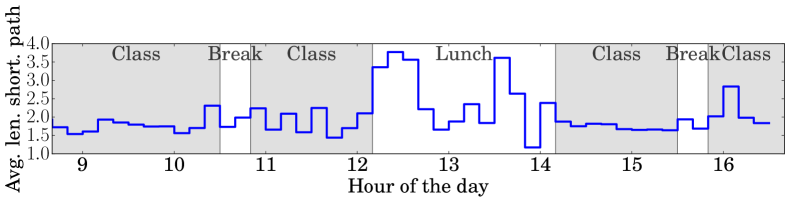
(d) Average length of shortest paths

Figure 8: Descriptors of the Primary School Temporal Network over time. The shaded regions correspond to class periods, while white regions correspond to breaks and lunch, according to the information given in [32]. No significant information are provided by the usual network-based descriptors

Figure 8 shows the network-based descriptors used to characterize the temporal network. Figures 8a and 8b show that the number of edges in the temporal network, as well as the number of isolated vertices, is not constant over time, reflecting the real-world nature of data: during the lunch break, some children leave the school to have lunch at home. The network-based descriptors (Figures 8c and Figures 8d) do not provide significant insights about the structure of the temporal network.

6.2 Spectral analysis

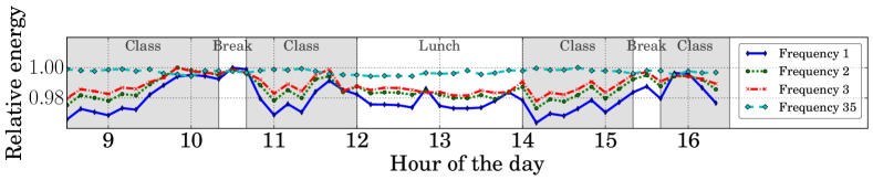
(a) Averaged over frequencies $\bm{E}_{f}(c)$ for $c\in\{0,1,2,70\}$

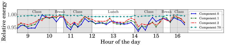
(b) Averaged over components $\bm{E}_{c}(f)$ for $f\in\{1,2,3,35\}$

Figure 9: Marginals of the energies of temporal spectra.The energies of the low frequencies and of the first components are not equally distributed over time, indicating changes in the global structure of the temporal network.

Figure 9 shows the marginals of the energies of temporal spectra obtained from the transformation of the primary school temporal network. The energies of the low frequencies and of the first components are not equally distributed over time: this indicates changes in the global structure of the temporal network, that occurs in break periods as well as during lunch. We can then divide the day into two main periods: the period where the children have class (shaded regions) and the breaks and lunch (white regions).

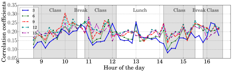
Figure 10: Correlation between the temporal spectra at each time step and the spectra of a network with a network with communities. Each line represent the number of communities, averaged over $20$ repetitions. The temporal network is correlated with structure with a large number of communities during class periods, and with structure with a small number of communities during breaks and lunch.

Comparing the Primary School Temporal Network with a network with communities using correlations between spectra shows that the former temporal network is correlated with the latter network involving a large number of communities (between 9 and 15) during class periods, a smaller one (between 3 and 6) during breaks and lunch periods (see Figure 10). This is consistent with the spatiotemporal trajectories given in [32], showing the location of the classes over time: during class periods, the classes are separated into different classrooms, while during breaks and lunch, the classes mix, yet in two distinct groups.

6.3 Decomposition into sub-networks

In the light of the above study of the temporal spectra, we can go further and decompose the Primary School Temporal Network into two temporal sub-networks. Furthermore, this allows for a quicker interpretation of the obtained components, as well as for an evidence of its ability the demonstration of the to extract the significant components.

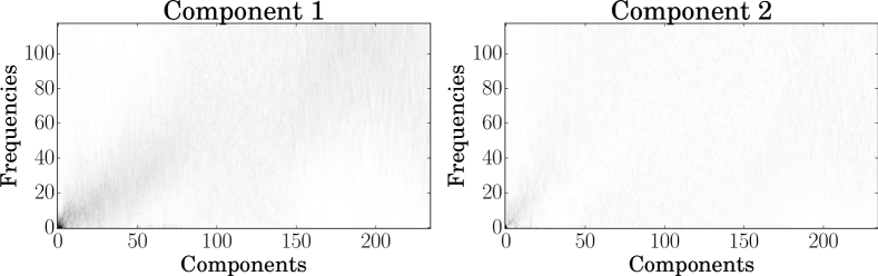
(a) Frequency patterns, obtained after reshaping the columns of $\bm{W}$ into matrices.

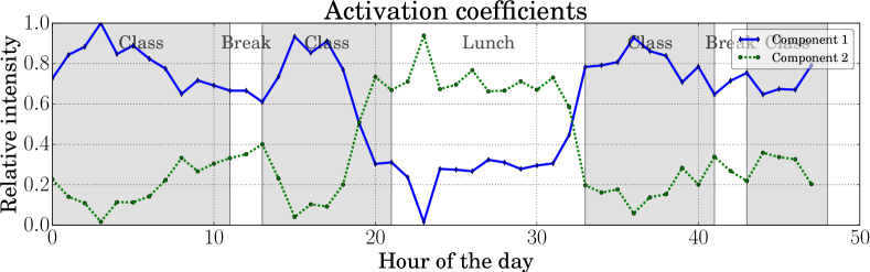
(b) Activation coefficients, corresponding to the rows of the matrix $\bm{H}$, normalized by the maximal value of $\bm{H}$

Figure 11: Results of the nonnegative matrix factorization for the Primary School Temporal Network, using $K=2$ and $\gamma=5$. The activation coefficients are consistent with the schedule of the children in the primary school, as detailed in [32].

Figure 11 shows the results of the NMF on the Primary School Temporal Network, using $K=2$ and $\gamma=5$. The school day is divided into three specific periods, according to the activation coefficients (Figure 11b). The first period occurs during class hours, where only the component $1$ is mainly active. The second period groups together the breaks, during which the components $1$ and $2$ are significantly present. Finally, the period $3$ concerns the lunch break, where the component $2$ is dominant. This cutting is consistent with the ground truth, as described in [32]: only two or three classes have breaks at the same time, while the other ones stay in their respective classrooms. As for lunches, they are taken in two consecutive turns, preserving the structure in classes, with nevertheless a weaker intensity.

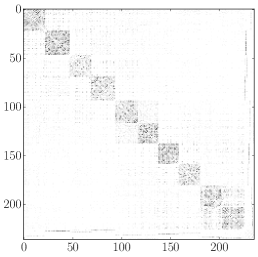
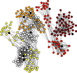
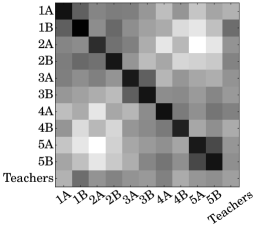
(a) Original temporal network

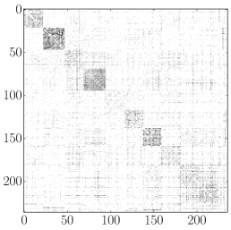
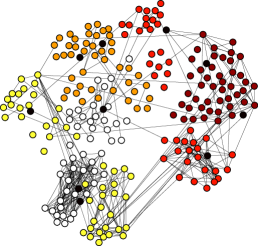
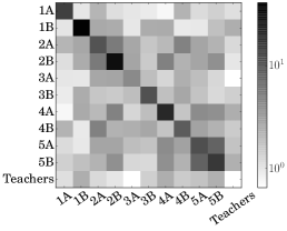
(b) Component 1

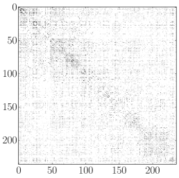
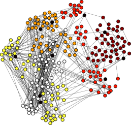
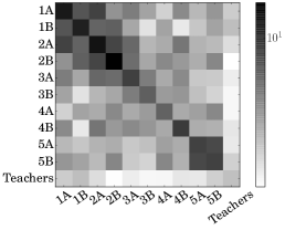
(c) Component 2

Figure 12: (Left) Aggregated adjacency matrix over time, weighted by the coefficients of $\bm{H}$. (Middle) Network representation using the layout provided in [32], after thresholding of edges according to their weights. The color of dots indicates the grade of the children, while black dots represent the teachers. (Right) Grayscale-coded contact matrix between classes: each entry gives the number of contacts inside and between the classes. A logarithmic scale is used to enhance the visualization. The component $1$ represents the structures in classes, while the component $2$ describes the structure during the breaks and lunch.

Figure 12 shows different representations of the temporal networks reconstructed from the components. The left figure shows the aggregated adjacency matrix over time, as described in Section 5.4. The vertices are ordered according to the classes of the children, from the youngest to the oldest. The middle figure shows the aggregated network, using the layout provided in [32], after thresholding of edges according to their weights. The color of dots indicates the grade of the children, while black dots represent the teachers. Finally, the right figure shows the contact matrix between classes, obtained by counting the number of edges inside and between the classes. A logarithmic scale is used to enhance the visualization. Figure 12a shows the original temporal network, while Figures 12b and 12c show respectively the component $1$ and the component $2$. We can easily observe that the component $1$ describes the structures in classes, with higher density of edges inside classes than between classes. Conversely, the component $2$ highlights a less structured network pattern, which looks like two communities, separating the youngest classes from the oldest. Those observations are consistent with the description of lunches mentioned above.

These results highlight the interest of decomposing a temporal network into several sub-networks, which can be studied independently of one another. Without prior knowledge, the different periods of activity in the primary school are displayed, and can then guide the analysis of the system by restricting the analysis over several time intervals.

7 Conclusion

We have proposed a novel method to track the structure of temporal networks over time using the duality between graphs and signals, as well as classical signal processing techniques, such as spectral analysis and nonnegative matrix factorization. At each time, the temporal network is represented by a graph which is transformed into a collection of signals. NMF is used to extract patterns in the energies of spectra of these signals; these patterns, whose activation coefficients vary over time, represent a specific structure of the underlying network. The effectiveness of the method has been demonstrated on a toy example, containing three types of structures as well as on a real-world network describing temporal contacts between children in a primary school.

These results provide insights in the characterization of temporal networks, but also call for further studies: In particular, it would be interesting to have a deeper look on how the reconstructed temporal networks are embedded in the original temporal network. Furthermore, it would be worth considering an iterative analysis, by studying the reconstructed temporal network themselves, using the same process. This could lead to a spatiotemporal multiscale analysis, permitting an increasingly precise track of the structure of the temporal network.

References

- [1] Ingwer Borg and Patrick J. F Groenen. Modern Multidimensional Scaling. Springer Series in Statistics. Springer, 2005.
- [2] D. Braha and Yaneer Bar-Yam. Time-dependent complex networks: Dynamic centrality, dynamic motifs, and cycles of social interactions. In Thilo Gross and Hiroki Sayama, editors, Adaptive Networks, Understanding Complex Systems, pages 39–50. Springer Berlin Heidelberg, 2009.
- [3] Andriana S. L. O. Campanharo, M. Irmak Sirer, R. Dean Malmgren, Fernando M. Ramos, and Luis A. N. Amaral. Duality between time series and networks. PloS one, 6(8), 2011.
- [4] Arnaud Casteigts, Paola Flocchini, Walter Quattrociocchi, and Nicola Santoro. Time-varying graphs and dynamic networks. International Journal of Parallel, Emergent and Distributed Systems, 27(5):387–408, 2012.
- [5] Yudong Chen, Vikas Kawadia, and Rahul Urgaonkar. Detecting overlapping temporal community structure in time-evolving networks. arXiv preprint arXiv:1303.7226, 2013.
- [6] Andrzej Cichocki. Era of big data processing: A new approach via tensor networks and tensor decompositions. arXiv preprint arXiv:1403.2048, 2014.
- [7] Andrea EF Clementi, Angelo Monti, Francesco Pasquale, and Riccardo Silvestri. Information spreading in stationary markovian evolving graphs. In IEEE International Symposium on Parallel & Distributed Processing, 2009, pages 1–12, 2009.
- [8] Slim Essid and Cédric Fevotte. Smooth nonnegative matrix factorization for unsupervised audiovisual document structuring. IEEE Transactions on Multimedia, 15(2):415–425, February 2013.
- [9] Cédric Févotte. Majorization-minimization algorithm for smooth itakura-saito nonnegative matrix factorization. In IEEE International Conference on Acoustics, Speech and Signal Processing (ICASSP), 2011, pages 1980–1983. IEEE, 2011.
- [10] Cédric Févotte, Nancy Bertin, and Jean-Louis Durrieu. Nonnegative matrix factorization with the itakura-saito divergence: With application to music analysis. Neural computation, 21(3):793–830, 2009.
- [11] Cédric Févotte and Jérôme Idier. Algorithms for nonnegative matrix factorization with the beta-divergence. Neural Computation, 23(9):2421–2456, June 2011.
- [12] S. Fortunato. Community detection in graphs. Physics Reports, 486(3):75–174, 2010.
- [13] Laetitia Gauvin, André Panisson, Alain Barrat, and Ciro Cattuto. Revealing latent factors of temporal networks for mesoscale intervention in epidemic spread. arXiv preprint arXiv:1501.02758, 2015.
- [14] Laetitia Gauvin, André Panisson, and Ciro Cattuto. Detecting the community structure and activity patterns of temporal networks: A non-negative tensor factorization approach. PLoS ONE, 9(1):e86028, 2014.
- [15] Benjamin Girault, Paulo Gonçalves, Eric Fleury, and Arashpreet Singh Mor. Semi-supervised learning for graph to signal mapping: a graph signal wiener filter interpretation. In IEEE International Conference on Acoustics Speech and Signal Processing (ICASSP), pages 1115–1119, Florence, Italy, 2014.
- [16] Peter Grindrod and Mark Parsons. Social networks: Evolving graphs with memory dependent edges. Physica A: Statistical Mechanics and its Applications, 390(21-22):3970–3981, October 2011.
- [17] Ronan Hamon, Pierre Borgnat, Patrick Flandrin, and Céline Robardet. Networks as signals, with an application to bike sharing system. In Global Conference on Signal and Information Processing (GlobalSIP), 2013 IEEE, pages 611–614, Austin, Texas, USA, 2013.
- [18] Ronan Hamon, Pierre Borgnat, Patrick Flandrin, and Céline Robardet. Tracking of a dynamic graph using a signal theory approach : application to the study of a bike sharing system. In ECCS’13, page 101, Barcelona, Spain, 2013.
- [19] Ronan Hamon, Pierre Borgnat, Patrick Flandrin, and Céline Robardet. Transformation de graphes dynamiques en signaux non stationnaires. In Colloque GRETSI 2013, page 251, Brest, France, 2013.
- [20] Ronan Hamon, Pierre Borgnat, Patrick Flandrin, and Céline Robardet. Nonnegative matrix factorization to find features in temporal networks. In IEEE International Conference on Acoustics Speech and Signal Processing (ICASSP), pages 1065–1069, Florence, Italy, 2014.
- [21] Ronan Hamon, Pierre Borgnat, Patrick Flandrin, and Céline Robardet. Discovering the structure of complex networks by minimizing cyclic bandwidth sum. Preprint arXiv:1410.6108, 2015.
- [22] Ronan Hamon, Pierre Borgnat, Patrick Flandrin, and Céline Robardet. From graphs to signals and back: Identification of graph structures using spectral analysis. Preprint arXiv:1502.04697, 2015.
- [23] Yuta Haraguchi, Yutaka Shimada, Tohru Ikeguchi, and Kazuyuki Aihara. Transformation from complex networks to time series using classical multidimensional scaling. In Artificial Neural Networks–ICANN 2009, pages 325–334. Springer, 2009.
- [24] Petter Holme and Jari Saramäki. Temporal networks. Physics reports, 519(3):97–125, 2012.
- [25] Lauri Kovanen, Márton Karsai, Kimmo Kaski, János Kertész, and Jari Saramäki. Temporal motifs in time-dependent networks. Journal of Statistical Mechanics: Theory and Experiment, 2011(11):P11005, November 2011.
- [26] Daniel D. Lee and H. Sebastian Seung. Learning the parts of objects by non-negative matrix factorization. Nature, 401(6755):788–791, October 1999.
- [27] Peter J. Mucha, Thomas Richardson, Kevin Macon, Mason A. Porter, and Jukka-Pekka Onnela. Community structure in time-dependent, multiscale, and multiplex networks. Science, 328(5980):876–878, May 2010.
- [28] Mark Newman. Networks: An Introduction. Oxford University Press, Inc., New York, NY, USA, 2010.
- [29] A. Sandryhaila and J.M.F. Moura. Discrete signal processing on graphs: Frequency analysis. Signal Processing, IEEE Transactions on, 62(12):3042–3054, June 2014.
- [30] Yutaka Shimada, Tohru Ikeguchi, and Takaomi Shigehara. From networks to time series. Phys. Rev. Lett., 109(15):158701, 2012.
- [31] David I. Shuman, Sunil K. Narang, Pascal Frossard, Antonio Ortega, and Pierre Vandergheynst. The emerging field of signal processing on graphs: Extending high-dimensional data analysis to networks and other irregular domains. IEEE Signal Processing Magazine, 30(3):83–98, 2013.
- [32] Juliette Stehlé, Nicolas Voirin, Alain Barrat, Ciro Cattuto, Lorenzo Isella, Jean-François Pinton, Marco Quaggiotto, Wouter Van den Broeck, Corinne Régis, Bruno Lina, and Philippe Vanhems. High-resolution measurements of face-to-face contact patterns in a primary school. PLoS ONE, 6(8):e23176, August 2011.
- [33] Nicolas Tremblay and Pierre Borgnat. Graph wavelets for multiscale community mining. IEEE Transactions on Signal Processing, 62(20):5227–5239, 2014.
- [34] Tongfeng Weng, Yi Zhao, Michael Small, and Defeng (David) Huang. Time-series analysis of networks: Exploring the structure with random walks. Physical Review E, 90(2):022804, 2014.
- [35] Kevin S. Xu and Alfred O. Hero III. Dynamic stochastic blockmodels: Statistical models for time-evolving networks. In Ariel M. Greenberg, William G. Kennedy, and Nathan D. Bos, editors, Social Computing, Behavioral-Cultural Modeling and Prediction, volume 7812 of Lecture Notes in Computer Science, pages 201–210. Springer Berlin Heidelberg, 2013.
- [36] Kevin S. Xu, Mark Kliger, and Alfred O. Hero. A regularized graph layout framework for dynamic network visualization. Data Mining and Knowledge Discovery, 27(1):84–116, July 2013.
- [37] Kevin S. Xu, Mark Kliger, and Alfred O. Hero III. Tracking communities in dynamic social networks. In Social Computing, Behavioral-Cultural Modeling and Prediction, pages 219–226. Springer, 2011.
- [38] B.-K. Yi, Nikolaos D. Sidiropoulos, Theodore Johnson, H. V. Jagadish, Christos Faloutsos, and Alexandros Biliris. Online data mining for co-evolving time sequences. In Data Engineering, 2000. Proceedings. 16th International Conference on, pages 13–22. IEEE, 2000.
- [39] Zhongyuan Zhang, Chris Ding, Tao Li, and Xiangsun Zhang. Binary matrix factorization with applications. In Data Mining, 2007. ICDM 2007. Seventh IEEE International Conference on, pages 391–400. IEEE, 2007.