Black Hole Radiation with Modified Dispersion Relation in Tunneling Paradigm: Static Frame

Abstract

To study possible deviations from the Hawking’s prediction, we assume that the dispersion relations of matter fields are modified at high energies and use the Hamilton-Jacobi method to investigate the corresponding effects on the Hawking radiation in this paper. The preferred frame is the static frame of the black hole. The dispersion relation adopted agrees with the relativistic one at low energies but is modified near the Planck mass $m_{p}$. We calculate the corrections to the Hawking temperature for massive and charged particles to $\mathcal{O}\left(m_{p}^{-2}\right)$ and massless and neutral particles to all orders. Our results suggest that the thermal spectrum of radiations near horizon is robust, e.g. corrections to the Hawking temperature are suppressed by $m_{p}$. After the spectrum of radiations near the horizon is obtained, we use the brick wall model to compute the thermal entropy of a massless scalar field near the horizon of a 4D spherically symmetric black hole. We find that the subleading logarithmic term of the entropy does not depend on how the dispersion relations of matter fields are modified. Finally, the luminosities of black holes are computed by using the geometric optics approximation.

I Introduction

The classical theory of black holes predicts that anything, including light, couldn’t escape from the black holes. However, Stephen Hawking demonstrated that quantum effects could allow black holes to radiate a thermal flux of quantum particles IN-Hawking:1974sw . The assumption that the ultra-high energy modes are in their ground state was used to derive the Hawking radiation in the framework of quantum field theory in curved spacetime. After this discovery, it was realized that there was the trans-Planckian problem with the calculation IN-Unruh:1976db . Due to the exponential high gravitational red shift near the horizon, the outgoing particles of the Hawking radiation originate from the extremely high (e.g., trans-Planckian) frequency modes. So the Hawking radiation relies on the validity of quantum field theory in curved spacetime to arbitrary high energies. On the other hand, quantum field theory is considered more like an effective field theory of an underlying theory whose nature remains unknown IN-Weinberg:1996kw . This observation poses the question of whether any unknown physics at the Planck scale could strongly influence the Hawking radiation.

It is believed that the trans-Planckian physics manifests itself in certain modifications of the existing models. Thus, even though a complete theory of quantum gravity is not yet available, we can use a “bottom-to-top approach” to probe the possible effects of quantum gravity on our current theories and experiments IN-AmelinoCamelia:2004hm . One possible way of how such an approach works is via Planck-scale modifications of the usual energy-momentum dispersion relation

$$p^{2}=E^{2}-m^{2},$$ (1)

whose possibility has been considered in the quantum-gravity literature IN-AmelinoCamelia:1997gz ; IN-Garay:1998wk ; IN-AmelinoCamelia:2002wr ; IN-Magueijo:2002am . The modified dispersion relation (MDR) has been reviewed in the framework of Lorentz violating theories in IN-Mattingly:2005re ; IN-Liberati:2013xla . It has also been shown that the MDR might play a role in astronomical and cosmological observations, such as the threshold anomalies of ultra high energy cosmic rays and TeV photons IN-AmelinoCamelia:1997gz ; IN-Colladay:1998fq ; IN-Coleman:1998ti ; IN-AmelinoCamelia:2000zs ; IN-Jacobson:2001tu ; IN-Jacobson:2003bn . Moreover, thermodynamics of black holes have been explored in the framework of the MDR IN-AmelinoCamelia:2004xx ; IN-Ling:2005bq ; IN-AmelinoCamelia:2005ik ; IN-Nozari:2006ka ; IN-Sefiedgar:2010we ; IN-Majumder:2011xg .

On the other hand, there are various methods for deriving the Hawking radiation and calculating its temperature. Among them is a semiclassical method of modeling Hawking radiation as a tunneling process. This method was first proposed by Kraus and Wilczek IN-Kraus:1994by ; IN-Kraus:1994fj , which is known as the null geodesic method. They employed the dynamical geometry approach to calculate the imaginary part of the action for the tunneling process of s-wave emission across the horizon and related it to the Boltzmann factor for the emission at the Hawking temperature. Later, the tunneling behaviors of particles were investigated using the Hamilton-Jacobi method IN-Srinivasan:1998ty ; IN-Angheben:2005rm ; IN-Kerner:2006vu . In the Hamilton-Jacobi method, one ignores the self-gravitation of emitted particles and assumes that its action satisfies the relativistic Hamilton-Jacobi equation. The tunneling probability for the classically forbidden trajectory from inside to outside the horizon is obtained by using the Hamilton-Jacobi equation to calculate the imaginary part of the action for the tunneling process. Using the null geodesic method and Hamilton-Jacobi method, much fruit has been achieved IN-Hemming:2001we ; IN-Medved:2002zj ; IN-Vagenas:2001rm ; IN-Arzano:2005rs ; IN-Wu:2006pz ; IN-Nadalini:2005xp ; IN-Chatterjee:2007hc ; IN-Akhmedova:2008dz ; IN-Akhmedov:2008ru ; IN-Akhmedova:2008au ; IN-Banerjee:2008ry ; IN-Singleton:2010gz . Furthermore, the effects of quantum gravity on the Hawking radiation have been discussed in the Hamilton-Jacobi method. In fact, the minimal length deformed Hamilton-Jacobi equation for fermions in curved spacetime have been introduced, and the modified Hawking temperatures have been derived IN-Chen:2013pra ; IN-Chen:2013tha ; IN-Chen:2013ssa ; IN-Chen:2014xsa ; IN-Chen:2014xgj ; IN-Mu:2015qta .

In order to introduce the modified dispersion relation we need to specify one special reference frame. The Hamilton-Jacobi equations were imported to curved spacetime using the static preferred frame in IN-Chen:2013pra ; IN-Chen:2013tha ; IN-Chen:2013ssa ; IN-Chen:2014xsa ; IN-Chen:2014xgj ; IN-Mu:2015qta , which leads us first to considering the static preferred frame in this paper. The models with free-fall preferred frame will be investigated in IN-Wang . Comparisons between the results in our paper and those in IN-Chen:2013pra ; IN-Chen:2013tha ; IN-Chen:2013ssa ; IN-Chen:2014xsa ; IN-Chen:2014xgj will be given at the end of the section II.

As shown in the appendix, specifying one special reference frame in the framework of the effective field theory is just picking up a vacuum expectation value (vev) for a vector field $u^{\mu}$. In static frame/free-fall frame scenario, the vev of $u^{\mu}$ is the unit vector field tangent to the static/free-fall observer’s world line. In the standard model, different vev of the Higgs field could give different results, e.g., the results in LHC and evolution of the universe. In this sense, it is not expected to have equivalent results from static and free-fall frame scenarios. In fact, a brief comparison between the results of this paper and those of free-fall scenario in IN-Wang is given in section VII, which shows that differences are found for these two scenarios. Just like that the vev of the Higgs field is determined by the results from LHC and other experiments, the vev of $u^{\mu}$ should be given by observational and experimental results. Before we can achieve this, every possible scenario deserves being explored.

It is noteworthy that the modified Hawking temperature, the atmosphere entropy in the brick wall model, and the spectrum of radiation of black holes due to the MDR have been widely investigated. In the following, we sum up what is new in our paper:

1. The modified Hawking temperature has been calculated in a heuristic method proposed in IN-AmelinoCamelia:2004xx ; IN-AmelinoCamelia:2005ik , which was similar to that introduced by Bekenstein IN-Bekenstein:1973ur . In a more rigorous way, the dispersive field theory models IN-Unruh:1994je ; IN-Brout:1995wp ; IN-Corley:1996ar ; IN-Corley:1997pr ; IN-Himemoto:1999kd ; IN-Saida:1999ap ; IN-Unruh:2004zk ; IN-Macher:2009tw ; IN-Coutant:2011in ; IN-Coutant:2014cwa ; IN-Belgiorno:2014bna have been proposed to study the effects on the Hawking radiation due to modifications of the dispersion relations of matter field at high energies. These models were motivated by a hydrodynamic analogue of a black hole radiation IN-Unruh:1994je . Similar to the original method for deriving the Hawking radiation, the energy fluxes for outgoing radiation were usually obtained by calculating the Bogoliubov transformations between the initial and final states of incoming and outgoing radiation. In these works, the Hawking temperature was only calculated up to the leading order. In our paper, we use the Hamilton-Jacobi method to study the dispersive field theory models and calculate the modified effective Hawking temperature beyond the leading order.

2. The modified Stefan-Boltzmann law and luminosities of black holes due to the MDR were discussed in IN-AmelinoCamelia:2005ik . We also calculate the modified luminosities of black holes in our paper. The geometric optics approximation are used in IN-AmelinoCamelia:2005ik and our paper. In such approximation, a 4D Schwarzschild black hole can be described as a black sphere of the radius $R$ and the temperature $T$. As a result, we consider effects of the MDR on both $R$ (see $r_{\min}$ in eqns. $\left(\ref{eq:R amd lamda min}\right)$) and $T$ in our paper. On the other hand, only effects of the MDR on $T$ were considered in IN-AmelinoCamelia:2005ik . Moreover, in our paper, we use detailed balance condition to show that the average number $n_{\omega,i}$ in the mode with the energy $\omega$ and other quantum numbers $i$ is

   $$n_{\omega,i}=n\left(\frac{\omega}{T_{eff}}\right),$$ (2)

   where $T_{eff}$ is the modified effective Hawking temperature depending on $\omega$. In contrast, the authors of IN-AmelinoCamelia:2005ik assumed an average behavior for particles described by a unique average temperature $T_{BH}$, which only depended on the black hole. Therefore in IN-AmelinoCamelia:2005ik , the average number $n_{\omega,i}$ was given by

   $$n_{\omega,i}=n\left(\frac{\omega}{T_{BH}}\right).$$ (3)

3. By using the brick wall model, the atmosphere entropy of radiation of a black hole was calculated in the framework of the MDR IN-Chang:2003sa and generalized uncertainty principle IN-Kim:2007if . In these works, only the effects of quantum gravity on the number of quantum states were considered. In our paper, we calculate the modified atmosphere entropy in the brick model by taking the effects of the MDR both on the number of quantum states and Hawking temperature into account.

The remainder of our paper is organized as follows. In section II, the deformed Hamilton-Jacobi equations incorporating the MDR are derived. In section IV, we solve the deformed Hamilton-Jacobi equations to obtain tunneling rates for massive and charged particles to $\mathcal{O}\left(m_{p}^{-2}\right)$ and massless and neutral particles to all orders. Thermodynamics of radiations near the horizon is discussed in section IV. The thermal entropy of a massless scalar field near the horizon is computed in section V by using the brick wall model. In section VI, we calculate luminosities of a 4D spherically symmetric black hole with the mass $M\gg m_{p}$ and a 2D one. Section VII is devoted to our discussion and conclusion, where the limitations of our calculations are discussed. Effective field theories incorporating the MDR are constructed in the appendix to obtain the deformed Hamilton-Jacobi equations. Throughout the paper we take Geometrized units $c=G=1$, where the Planck constant $\hbar$ is square of the Planck Mass $m_{p}$.

II Deformed Hamilton-Jacobi Equation

In most cases, the MDR could take the form of

$$p^{2}=m_{p}^{2}H\left(\frac{E}{m_{p}},\frac{m}{m_{p}}\right),$$ (4)

where $m_{p}$ is Planck mass and $H\left(x,y\right)=x^{2}-y^{2}$ for the unmodified dispersion relation. Taylor expanding the right-hand side of eqn. $\left(\ref{eq:ExactMDR}\right)$ for $E,m\ll m_{p}$ gives

$$p^{2}=\sum_{i,j=0}^{\infty}h_{i,j}\frac{E^{i}m^{i}}{m_{p}^{i+j-2}},$$ (5)

where $h_{i,j}$ is the coefficient of $x^{i}y^{j}$ in the Taylor series of $H\left(x,y\right)$ evaluated at $\left(0,0\right)$. Since eqn. $\left(\ref{eq:MDRExpansionH}\right)$ has to become eqn. $\left(\ref{eq:uMDR}\right)$ when $m_{p}\rightarrow\infty$, we find

$$h_{0,0}=h_{0,1}=h_{1,0}=h_{1,1}=0\text{ and }h_{2,0}=h_{0,2}=1\text{.}$$ (6)

After some manipulations, eqn. $\left(\ref{eq:MDRExpansionH}\right)$ can be put in the form of

$$p^{2}=\alpha\left(\frac{m}{m_{p}}\right)E^{2}-\beta\left(\frac{m}{m_{p}}\right)m^{2}+\gamma\left(\frac{m}{m_{p}}\right)mE+\sum_{n\geq 3}\frac{C_{n}\left(\frac{m}{m_{p}}\right)E^{n}}{m_{p}^{n-2}},$$ (7)

where $\alpha\left(0\right)=\beta\left(0\right)=1$ and $\gamma\left(0\right)=0$.  If the modifications to the dispersion relation are suppressed by some the scale of Lorentz violation $\Lambda,$ the naturalness in effective field theories would imply that $C_{n}\sim\left(\frac{m_{p}}{\Lambda}\right)^{n}$. For $\Lambda\ll m_{p}$, $C_{n}$ could become much large. To include a broader class, we consider a static black hole in the possible presence of electromagnetic potential $A_{\mu}$ with the line element

$$ds^{2}=f\left(r\right)dt^{2}-\frac{1}{f\left(r\right)}dr^{2}-C\left(r^{2}\right)h_{ab}\left(x\right)dx^{a}dx^{b},$$ (8)

where $f\left(r\right)$ has a simple zero at $r=r_{h}$ with $f^{\prime}\left(r_{h}\right)$ being finite and nonzero. The vanishing of $f\left(r\right)$ at point $r=r_{h}$ indicates the presence of an event horizon. We also assume that the vector potential $A_{\mu}$ is given by

$$A_{\mu}=A_{t}\left(r\right)\delta_{\mu t},$$ (9)

which is true for charged static black holes in most cases.

The MDR breaks the Lorentz invariance in flat spacetime. Thus, one needs to pick up a preferred frame to determine the form of the MDR. The energy and momentum in eqn. $\left(\ref{eq:MDRExpansion}\right)$ are defined with respect to the preferred frame, where can be described by the unit vector $u^{\mu}$ tangent to the observers’ world lines. Explicitly, we have

$$E =p_{\mu}u^{\mu},$$

$$p^{2} =E^{2}-p_{\mu}p^{\mu},$$ (10)

where $p_{\mu}$ is the energy-momentum vector and $E$ and $p$ are the energy and the norm of the momentum measured in the preferred reference frame, respectively. When introducing the MDR into curved spacetime, we use the vector field $u^{\mu}\left(x_{\nu}\right)$. To obtain the deformed Hamilton-Jacobi equation incorporating the MDR, it is necessary to specify the profile of the preferred frame in the black hole spacetime. One of natural frames is a static frame hovering above the black hole. For such a frame, the vector field $u^{\mu}\left(x_{\nu}\right)$ is

$$u^{\mu}\left(x_{\nu}\right)=\left(\sqrt{g^{tt}},\vec{0}\right)=\left(\frac{1}{\sqrt{f\left(r\right)}},\vec{0}\right).$$ (11)

Plugging eqn. $\left(\ref{eq:4velocity}\right)$ into eqns. $\left(\ref{eq:energy and momentum}\right)$, one finds that the energy and the magnitude of the momentum becomes

$$E =\frac{p_{t}}{\sqrt{f\left(r\right)}},$$

$$p^{2} =f\left(r\right)p_{r}^{2}+\frac{h^{ab}\left(x\right)}{C\left(r^{2}\right)}p_{a}p_{b}.$$ (12)

It can be shown that, if the classical action $I$ is a solution of the Hamilton-Jacobi equation, then the transformation equations give

$$p_{\mu}=-\partial_{\mu}I,$$ (13)

where $-$ appears since $p_{\mu}=\left(E,-\vec{p}\right)$ in our metric signature. Furthermore, since $\partial_{t}$ is a Killing vector of the background spacetime, $\left(\partial_{t}\right)^{\mu}p_{\mu}=p_{t}$ is a constant. In fact, $p_{t}$ is the conserved energy of the particle, and we define $\omega\equiv$ $p_{t}=-\partial_{t}I$, which means we can separate $t$ from other variables. Relating $I$ to $p_{\mu}$ via eqn. $\left(\ref{eq:transformation-eqn}\right)$ and putting eqns. $\left(\ref{eq:energy-momentum-BH}\right)$ into eqn. $\left(\ref{eq:MDRExpansion}\right)$ give the deformed Hamilton-Jacobi equation. In the appendix, the deformed Hamilton-Jacobi equation is also derived in a more rigorous way, specifically in the language of the effective field theory. We show there that if a scalar/fermion obeys the MDR given in eqn. $\left(\ref{eq:MDRExpansion}\right)$ in flat spacetime, the deformed scalar/fermionic Hamilton-Jacobi equation with respect to the preferred static frame in the black hole background spacetime can be both written as

$$X^{2}=\alpha\left(\frac{m}{m_{p}}\right)T^{2}-\beta\left(\frac{m}{m_{p}}\right)m^{2}+\gamma\left(\frac{m}{m_{p}}\right)mT+\sum_{n\geq 3}\frac{C_{n}\left(\frac{m}{m_{p}}\right)T^{n}}{m_{p}^{n-2}},$$ (14)

where we define

$$T=-\frac{\partial_{t}I+qA_{t}}{\sqrt{f\left(r\right)}},X^{2}=f\left(r\right)\left(\partial_{r}I\right)^{2}+\frac{h^{ab}\left(x\right)\partial_{a}I\partial_{b}I}{C\left(r^{2}\right)},$$ (15)

$A_{\mu\text{ }}$is the black hole’s electromagnetic potential and $q$ is the particle’s charge.

III Tunneling Rate

In this section, we use the Hamilton-Jacobi method to investigate the particles’ tunneling across the event horizon $r=r_{h}$ of the metric $\left(\ref{eq:BHmetric}\right)$ by solving eqn. $\left(\ref{eq:deformedHJeqn}\right)$. Taking into account $\partial_{t}I=-\omega$, we can employ the following ansatz for the action $I$

$$I=-\omega t+W\left(r\right)+\Theta\left(x\right),$$ (16)

where $\omega$ is the particle’s energy. Plugging the ansatz into eqn. $\left(\ref{eq:TandX}\right)$, we have

$$T =\frac{\omega-qA_{t}\left(r\right)}{\sqrt{f\left(r\right)}},$$

$$X^{2} =f\left(r\right)\left[\partial_{r}W\left(r\right)\right]^{2}+\frac{h^{ab}\left(x\right)\partial_{a}\Theta\left(x\right)\partial_{b}\Theta\left(x\right)}{C\left(r^{2}\right)}.$$ (17)

The method of separation of variables gives the differential equation for $\Theta\left(x\right)$

$$h^{ab}\left(x\right)\partial_{a}\Theta\left(x\right)\partial_{b}\Theta\left(x\right)=\lambda,$$ (18)

where is $\lambda$ is a constant and determined by $h^{ab}\left(x\right)$. Thus, one has

$$X^{2}=f\left(r\right)\left[\partial_{r}W\left(r\right)\right]^{2}+\frac{\lambda}{C\left(r^{2}\right)},$$ (19)

and eqn. $\left(\ref{eq:deformedHJeqn}\right)$ becomes an ordinary differential equation for $W\left(r\right)$. In this section, we solve eqn. $\left(\ref{eq:deformedHJeqn}\right)$ for $\partial_{r}W\left(r\right)$, calculate its residue at $r=r_{h}$ and find the imaginary part of $I$ which gives the tunneling rate $\Gamma$ across the event horizon. We will calculate $\operatorname{Im}W$ for two cases, a massive and charged particle to $\mathcal{O}\left(m_{p}^{-2}\right)$ and a neutral and massless particle to all orders.

III.1 Massive and Charged Particle to $\mathcal{O}\left(m_{p}^{-2}\right)$

Consider a particle with the mass $m$ and the charge $q$. Solving eqn. $\left(\ref{eq:deformedHJeqn}\right)$ for $p_{r}\equiv\partial_{r}W\left(r\right)$ gives

$$p_{r}^{{}_{\pm}} =\frac{\pm 1}{\sqrt{f\left(r\right)}}\left(\alpha\left(\frac{m}{m_{p}}\right)\frac{\tilde{\omega}^{2}\left(r\right)}{f\left(r\right)}-\beta\left(\frac{m}{m_{p}}\right)m^{2}-\frac{\lambda}{C\left(r^{2}\right)}+m\gamma\left(\frac{m}{m_{p}}\right)\frac{\tilde{\omega}\left(r\right)}{\sqrt{f\left(r\right)}}\right)^{\frac{1}{2}}$$

$$\left(1+\frac{1}{\alpha\left(\frac{m}{m_{p}}\right)\frac{\tilde{\omega}^{2}\left(r\right)}{f\left(r\right)}-\beta\left(\frac{m}{m_{p}}\right)m^{2}-\frac{\lambda}{C\left(r^{2}\right)}+m\gamma\left(\frac{m}{m_{p}}\right)\frac{\tilde{\omega}\left(r\right)}{\sqrt{f\left(r\right)}}}{\displaystyle\sum\limits_{n\geq 3}}\frac{C_{n}\left(\frac{m}{m_{p}}\right)}{m_{p}^{n-2}}\frac{\tilde{\omega}^{n}\left(r\right)}{f\left(r\right)^{\frac{n}{2}}}\right)^{\frac{1}{2}},$$ (20)

where $+$/$-$ denotes the outgoing/ingoing solutions, and $\tilde{\omega}\left(r\right)\equiv\omega-qA_{t}\left(r\right)$. Here, we have a pole at $r=r_{h}$. Using the residue theory for the semi circle${}^{\left[\ref{footnote}\right]}$, we get

$$\operatorname{Im}W_{\pm}\left(r\right)=\pm\frac{\sqrt{\alpha}\tilde{\omega}\left(r_{h}\right)\pi}{2\kappa}\left(1+\Delta_{qm}+\mathcal{O}\left(m_{p}^{-3}\right)\right),$$ (21)

where we define $\kappa=f^{\prime}\left(r_{h}\right)/2$ and

$$\Delta_{qm} =-\frac{C_{3}m\gamma}{4m_{p}\alpha^{2}}+\frac{1}{32m_{p}^{2}\kappa\alpha^{4}}\left[\left(24C_{4}\alpha-6C_{3}^{2}\right)\tilde{\omega}^{\prime}\left(r_{h}\right)\tilde{\omega}\left(r_{h}\right)\alpha^{2}+\kappa m^{2}\gamma^{2}\frac{12C_{4}\alpha-15C_{3}^{2}}{2}\right.$$

$$\left.-\kappa\alpha\left(6C_{3}^{2}-8C_{4}\alpha\right)\left(\frac{\lambda}{C\left(r_{h}^{2}\right)}+\beta m^{2}\right)+\alpha^{2}\left(C_{3}^{2}-4C_{4}\alpha\right)\frac{f^{\prime\prime}\left(r_{h}\right)\tilde{\omega}^{2}\left(r_{h}\right)}{\kappa}\right].$$ (22)

The argument $\frac{m}{m_{p}}$ is suppressed for $\alpha\left(\frac{m}{m_{p}}\right)$, $\beta\left(\frac{m}{m_{p}}\right)$, $\gamma\left(\frac{m}{m_{p}}\right)$ and $C_{n}\left(\frac{m}{m_{p}}\right)$ in eqns. $\left(\ref{eq:ImW}\right)$ and $\left(\ref{eq:delta}\right).$

III.2 Massless and Neutral Particle to All Orders

We now work with a particle with $m=0$ and $q=0$. Solving eqn. $\left(\ref{eq:deformedHJeqn}\right)$ for $p_{r}$ gives

$$p_{r}^{{}_{\pm}}=\frac{\pm 1}{\sqrt{f\left(r\right)}}\left(\frac{\omega^{2}}{f\left(r\right)}-\frac{\lambda}{C\left(r^{2}\right)}\right)^{\frac{1}{2}}\left(1+\frac{1}{\frac{\omega^{2}}{f\left(r\right)}-\frac{\lambda}{C\left(r^{2}\right)}}{\displaystyle\sum\limits_{n\geq 3}}\frac{C_{n}}{m_{p}^{n-2}}\frac{\omega^{n}}{f\left(r\right)^{\frac{n}{2}}}\right)^{\frac{1}{2}},$$ (23)

where $C_{n}\equiv C_{n}\left(0\right)$ and we use $\alpha\left(0\right)=1.$ To get the residue of $p_{r}^{{}_{\pm}}$ at $r=r_{h}$, we first define a few coefficients $C_{n}^{\alpha}$, $\tilde{C}_{m,n}$, and $\eta_{l}^{k}$ as follows

$$\left(1+x\right)^{\alpha} ={\displaystyle\sum\limits_{n\geq 0}}C_{n}^{\alpha}x^{n},$$

$$\left({\displaystyle\sum\limits_{n=0}^{\infty}}C_{n+3}x\right)^{m} ={\displaystyle\sum\limits_{n=0}^{\infty}}\tilde{C}_{m,n}x^{n},$$

$$\eta_{l}^{k} ={\displaystyle\sum\limits_{m=0}^{k}}\left(-1\right)^{l}C_{m}^{\frac{1}{2}}C_{l}^{-m+\frac{1}{2}}\tilde{C}_{m,k-m},$$ (24)

where $m$ is a non-negative integer, and $C_{n}^{\alpha}$ are generalized binomial coefficients with $C_{n}^{\alpha}={\displaystyle\prod\limits_{k=1}^{n}}\frac{\alpha-k+1}{k}$. Therefore, one has

$$p_{r}^{\pm} =\pm{\displaystyle\sum\limits_{m=0}^{\infty}}\frac{\omega^{m}}{m_{p}^{m}f^{\frac{m}{2}}\left(r\right)}\frac{C_{m}^{\frac{1}{2}}\omega}{f\left(r\right)}\left(1-\frac{f\left(r\right)\lambda}{C\left(r^{2}\right)\omega^{2}}\right)^{-m+\frac{1}{2}}\left({\displaystyle\sum\limits_{n=0}^{\infty}}\frac{C_{n+3}}{m_{p}^{n}}\frac{\omega^{n}}{f^{\frac{n}{2}}\left(r\right)}\right)^{m}$$

$$=\pm\frac{\omega}{f\left(r\right)}{\displaystyle\sum\limits_{l=0}^{\infty}}{\displaystyle\sum\limits_{k=0}^{\infty}}\frac{\lambda^{l}}{C^{l}\left(r^{2}\right)}\frac{\eta_{l}^{k}}{m_{p}^{k}}\frac{\omega^{k-2l}}{f^{\frac{k}{2}-l}\left(r\right)}$$

$$\sim\pm\frac{\omega}{f\left(r\right)}{\displaystyle\sum\limits_{l=0}^{\infty}}{\displaystyle\sum\limits_{k=0}^{\infty}}\frac{\lambda^{l}}{C^{l}\left(r^{2}\right)}\frac{\eta_{l}^{2k+2l}}{m_{p}^{2k+2l}}\frac{\omega^{2k}}{f^{k}\left(r\right)}$$

$$\sim\pm\omega{\displaystyle\sum\limits_{l=0}^{\infty}}\left[\frac{\lambda}{C\left(r_{h}^{2}\right)m_{p}^{2}}\right]^{l}{\displaystyle\sum\limits_{k=0}^{\infty}}\eta_{l}^{2k+2l}\frac{\omega^{2k}}{m_{p}^{2k}}\left(\frac{C^{l}\left(r_{h}^{2}\right)}{C^{l}\left(r^{2}\right)}\frac{1}{f^{k+1}\left(r\right)}\right),$$ (25)

where we only keep terms contributing to the residue and set $k\rightarrow k+2l$ in the third line. Furthermore, we denote the residue of $\frac{C^{l}\left(r_{h}^{2}\right)}{C^{l}\left(r^{2}\right)}\frac{1}{f^{k+1}\left(r\right)}$ at $r=r_{h}$ by

$$\text{Res}\left(\frac{C^{l}\left(r_{h}^{2}\right)}{C^{l}\left(r^{2}\right)}\frac{1}{f^{k+1}\left(r\right)},r_{h}\right)=\frac{\zeta_{k}^{l}}{2\kappa}.$$ (26)

Using the residue theory for the semi circle, one has

$$\operatorname{Im}W_{\pm}\left(r\right)=\pm\frac{\omega\pi}{2\kappa}\left(1+\Delta\right),$$ (27)

where

$$\Delta={\displaystyle\sum\limits_{l+k\geq 1}^{\infty}}\left[\frac{\lambda}{C\left(r_{h}^{2}\right)m_{p}^{2}}\right]^{l}\eta_{l}^{2k+2l}\zeta_{k}^{l}\frac{\omega^{2k}}{m_{p}^{2k}}.$$ (28)

Note that $\eta_{0}^{0}=\zeta_{0}^{0}=1.$

III.3 Calculating $\lambda$

It is easy to see that $\lambda$ depends on $h_{ab}\left(x\right).$ Here we consider two kinds of black holes, 4D cylindrically and spherically symmetric black holes. For a 4D cylindrically symmetric black hole, we have

$$h_{ab}\left(x\right)dx^{a}dx^{b}=d\theta^{2}+\alpha^{2}dz^{2},$$ (29)

where $-\infty<z<\infty,$ $0\leq\theta\leq 2\pi$, and $\alpha$ is some constant. Since $\partial_{\theta}$ and $\partial_{z}$ are the Killing fields of the background spacetime, we can separate the variables and consider a solution for eqn. $\left(\ref{eq:HJh}\right)$ of the form

$$\Theta=J_{\theta}\theta+J_{z}z,$$ (30)

where $J_{\theta}$ and $J_{z}$ are constant, and $J_{\theta}$ is the angular momentum along $z$-axis. The periodicity of $\theta$ gives $J_{\theta}=n\hbar$ with $n\in Z$. Thus, one finds

$$\lambda=J_{\theta}^{2}+\frac{J_{z}^{2}}{\alpha^{2}},$$ (31)

where $J_{\theta}=n\hbar$ with $n\in Z$.

For a 4D spherically symmetric black hole, we have

$$h_{ab}\left(x\right)dx^{a}dx^{b}=d\theta^{2}+\sin^{2}\theta d\phi^{2},$$ (32)

where $0\leq\theta\leq\pi$ and $0\leq\phi\leq 2\pi$. $\partial_{\phi}$ is the Killing vector so we consider a solution for eqn. $\left(\ref{eq:HJh}\right)$ of the form

$$\Theta=Y\left(\theta\right)+J_{\phi}\phi,$$ (33)

where $J_{\phi}$ is the angular momentum along $z$-axis. The periodicity of $\phi$ gives $J_{\phi}=m\hbar$ with $m\in Z$ . Since the magnitude of the angular momentum of the particle $L$ can be expressed in terms of $p_{\theta}\equiv\partial_{\theta}Y\left(\theta\right)$ and $J_{\phi},$

$$L^{2}=p_{\theta}^{2}+\frac{p_{\phi}^{2}}{\sin^{2}\theta},$$ (34)

eqn. $\left(\ref{eq:HJh}\right)$ gives $\lambda=L^{2}$. Putting eqn. $\left(\ref{eq:theta}\right)$ into eqn. $\left(\ref{eq:HJh}\right)$, one gets

$$p_{\theta}=\sqrt{\lambda-\frac{m^{2}\hbar^{2}}{\sin^{2}\theta}}.$$ (35)

On the other hand, the Sommerfeld quantization for $p_{\theta}$ gives

$${\displaystyle\oint}d\theta p_{\theta}=2\pi\left(n+\frac{1}{2}\right)\hbar,$$ (36)

where $n$ is a non-negative integer. The integral in eqn. $\left(\ref{eq:sommerfeldquantization}\right)$ is calculated in the classically allowed region where $p_{\theta}$ is real, which requires that $\lambda\geq m^{2}\hbar^{2}$. Since the integral is taken over the whole period of the classical motion, the left-hand side of eqn. $\left(\ref{eq:sommerfeldquantization}\right)$ is given by

$${\displaystyle\oint}d\theta p_{\theta}=\int_{\arcsin\frac{\left|m\right|\hbar}{\sqrt{\lambda}}}^{\pi-\arcsin\frac{\left|m\right|\hbar}{\sqrt{\lambda}}}p_{\theta}^{+}d\theta+\int_{\pi-\arcsin\frac{\left|m\right|\hbar}{\sqrt{\lambda}}}^{\arcsin\frac{\left|m\right|\hbar}{\sqrt{\lambda}}}p_{\theta}^{-}d\theta=2\int_{\arcsin\frac{\left|m\right|\hbar}{\sqrt{\lambda}}}^{\pi-\arcsin\frac{\left|m\right|\hbar}{\sqrt{\lambda}}}p_{\theta}d\theta,$$ (37)

where $p_{\theta}^{+}=p_{\theta}$ and $p_{\theta}^{-}=-p_{\theta}$. Integrating the quantization integral, one finds that eqn. $\left(\ref{eq:sommerfeldquantization}\right)$ becomes

$$2\pi\left(\sqrt{\lambda}-\left|m\right|\hbar\right)=2\pi\left(n+\frac{1}{2}\right)\hbar.$$ (38)

Solving eqn. $\left(\ref{eq:lamda}\right)$ for $\lambda$ gives the WKB leading quantization of the angular momentum

$$\lambda=\left(l+\frac{1}{2}\right)^{2}\hbar^{2},$$ (39)

where $l=n+\left|m\right|=0,1,\cdots$ with $\left|m\right|\leq l$. Note that the difference between the exact quantization of the angular momentum $L^{2}=l\left(l+1\right)\hbar^{2}$ and the WKB leading quantization $L^{2}=\left(l+\frac{1}{2}\right)^{2}\hbar^{2}$ is $\frac{\hbar^{2}}{4}$.

III.4 Tunneling Rate

When one calculates the quantum tunneling rate from $\operatorname{Im}W_{\pm}$, there is so called “factor-two problem” TR-Akhmedov:2006pg . Thus, one may have a black hole temperature which is twice the expected result. One of solutions is proposed by Mitra TR-Mitra:2006qa . Mitra noted that in general, the action $I$ could include some complex constant of integration $\mathcal{K}$. In this way, the imaginary part of $I$ becomes

$$\operatorname{Im}I_{\pm}=\operatorname{Im}W_{\pm}+\operatorname{Im}\mathcal{K}$$ (40)

$+$/$-$ denotes the outgoing/ingoing solutions. In the semi-classical method, the absorption probability and the emission probability for a black hole are given by

$$P_{emit} \propto\exp\left(-\frac{2}{\hbar}\operatorname{Im}I_{+}\right)=\exp\left[-\frac{2}{\hbar}\left(\operatorname{Im}W_{+}+\operatorname{Im}\mathcal{K}\right)\right],$$

$$P_{abs} \propto\exp\left(-\frac{2}{\hbar}\operatorname{Im}I_{-}\right)=\exp\left[-\frac{2}{\hbar}\left(\operatorname{Im}W_{-}+\operatorname{Im}\mathcal{K}\right)\right].$$ (41)

On the other hand, it is noted that the classical theory of black holes tells us that an incoming particle is absorbed with the probability equalling to one. Thus, one can choose $\mathcal{K}$ to impose the classical constraint on the absorption probability, which is $\operatorname{Im}\mathcal{K=-}\operatorname{Im}W_{-}$. So eqn. $\left(\ref{eq:abs}\right)$ gives that the probability of a particle tunneling from inside to outside the horizon is

$$P_{emit}\propto\exp\left[-\frac{2}{\hbar}\left(\operatorname{Im}W_{+}-\operatorname{Im}W_{-}\right)\right].$$ (42)

Another way to circumvent this problem is considering both the contributions from spatial and temporal parts of the action to the tunneling rates.

Spatial Contribution: Along an open path in phase spaces of two canonically equivalent frames, one in general has that

$$\int pdx\neq\int PdX.$$ (43)

Therefore, $\operatorname{Im}W_{\pm}=\operatorname{Im}\int p_{r}^{\pm}dr$ used in eqns. $\left(\ref{eq:abs}\right)$ are not invariant under canonical transformations. On the other hand, a closed contour integral ${\displaystyle\oint}pdx$ is invariant under canonical transformations. It was then suggested  TR-Akhmedov:2006pg ; TR-Akhmedova:2008au ; TR-Chowdhury:2006sk that the tunneling rates could be given by

$$P_{emit/abs}\propto\exp\left(\pm\frac{1}{\hbar}\operatorname{Im}{\displaystyle\oint}p_{r}dr\right)\text{,}$$ (44)

where ${\displaystyle\oint}p_{r}dr=\int p_{r}^{+}dr-\int p_{r}^{-}dr$. It showed that eqns. $\left(\ref{eq:prob-emit}\right)$ and $\left(\ref{eq:RP}\right)$ yielded different results for the Schwarzschild spacetime in Painleve-Gulstrand coordinates TR-Akhmedova:2008au and thin shells from black holes TR-Chowdhury:2006sk . Eqn. $\left(\ref{eq:RP}\right)$ is preferred over eqn. $\left(\ref{eq:prob-emit}\right)$ since eqn. $\left(\ref{eq:RP}\right)$ is a proper observable. When $p_{r}^{\pm}$ have the same magnitude but opposite signs, eqns. $\left(\ref{eq:prob-emit}\right)$ and $\left(\ref{eq:RP}\right)$ give the same results.

Temporal Contribution: As shown in TR-Chowdhury:2006sk ; TR-Akhmedova:2008dz ; TR-deGill:2010nb , the temporal part contribution came from the ”rotation” which connects the interior region and the exterior region of the black hole. It was found in TR-deGill:2010nb that the direction in which the horizon was crossed did not affect the sign of the temporal contribution. However, the sign of the spatial contribution changed when the direction was reversed. Thus, the temporal contributions to $P_{emit/abs}$ were the same. When the horizon was crossed once, the action $I$ got a contribution of $\operatorname{Im}\left(\omega\Delta t\right)=\frac{\pi\omega}{2\kappa}$, and for a round trip, the total contribution was $\operatorname{Im}\left(\omega\Delta t\right)=\frac{\pi\omega}{\kappa}.$

Taking into account the spatial and temporal contributions, one has for the absorption probability

$$P_{abs}\propto\exp\left[-\frac{1}{\hbar}\left(-\operatorname{Im}{\displaystyle\oint}p_{r}dr+\operatorname{Im}\left(\omega\Delta t\right)+\operatorname{Im}\mathcal{K}\right)\right],$$ (45)

and for the emission probability

$$P_{emit}\propto\exp\left[-\frac{1}{\hbar}\left(\operatorname{Im}{\displaystyle\oint}p_{r}dr+\operatorname{Im}\left(\omega\Delta t\right)+\operatorname{Im}\mathcal{K}\right)\right],$$ (46)

where $\mathcal{K}$ is a constant of integration. Imposing the classical constraint on the absorption probability, one gets

$$\operatorname{Im}\mathcal{K}=\operatorname{Im}{\displaystyle\oint}p_{r}dr-\operatorname{Im}\left(\omega\Delta t\right),$$ (47)

and

$$P_{emit}\propto\left[-\frac{2}{\hbar}\left(\operatorname{Im}{\displaystyle\oint}p_{r}dr\right)\right]=\exp\left[-\frac{2}{\hbar}\left(\operatorname{Im}W_{+}-\operatorname{Im}W_{-}\right)\right].$$ (48)

Both approaches give the same expression for $P_{emit}$. There is a Boltzmann factor in $P_{emit}$ with an effective temperature. Using eqns. $\left(\ref{eq:ImW}\right)$ and $\left(\ref{eq:ImW-massless}\right),$ we find that the effective temperature for a massive and charged particle is

$$T_{eff}=\frac{T_{0}}{\sqrt{\alpha}\left(1+\Delta_{qm}\right)}+\mathcal{O}\left(m_{p}^{-3}\right),$$ (49)

and, that for a massless and neutral particle is

$$T_{eff}=\frac{T_{0}}{1+\Delta},$$ (50)

where we define $T_{0}=\frac{\hbar\kappa}{2\pi}$ and take $k_{B}=1$.

III.5 Discussion

In this section, we suppose that outgoing particles tunnel from $r_{1}<r_{h}$ to $r_{2}>r_{h}$ while ingoing particles from $r_{2}$ to $r_{1}$. To to obtain the imaginary part of $I$ for the tunneling process, we have to give an prescription for evaluating the integrals of $\operatorname{Im}W_{\pm}=\int_{r_{1}}^{r_{2}}p_{r}^{\pm}dr$. Following the Feynman’s $i\epsilon$–prescription TR-Vanzo:2011wq , we take the contour of the integral to be an infinitesimal semicircle below the pole at $r=r_{h}$ for outgoing particles. Thus, the integral becomes

$$\int_{r_{1}}^{r_{2}}p_{r}^{+}dr=\int_{r_{1}}^{r_{h}-\varepsilon}p_{r}^{+}dr+\int_{C_{B,\varepsilon}}p_{r}^{+}dr+\int_{r_{h}+\varepsilon}^{r_{2}}p_{r}^{+}dr,$$ (51)

where we denote the semicircle centered at $r=r_{h}$ with the radius of $R$ going from $r_{h}+R/r_{h}-R$ to $r_{h}-R/r_{h}+R$ in the upper/lower half complex plane by $C_{U/B,R}$. Since the contributions from the ranges $\left(r_{1},r_{h}-\varepsilon\right)$ and $\left(r_{h}+\varepsilon,r_{2}\right)$ are real, the imaginary part of $W_{+}$ is

$$\operatorname{Im}W_{+}=\operatorname{Im}\int_{C_{B,\varepsilon}}p_{r}^{+}dr.$$ (52)

Similarly, one has for ingoing particles

$$\operatorname{Im}W_{-}=\operatorname{Im}\int_{C_{U,\varepsilon}}p_{r}^{-}dr.$$ (53)

To get $\operatorname{Im}W_{\pm}$, we expand $p_{r}^{\pm}$ in powers of $\frac{\omega}{\sqrt{f\left(r\right)}m_{p}}$

$$p_{r}^{\pm}=\sum_{n\geq 0}\frac{\omega^{n+1}p_{n}^{\pm}\left(r\right)}{f^{\frac{n}{2}+1}\left(r\right)m_{p}^{n}},$$ (54)

where $p_{n}^{\pm}\left(r\right)$ are some analytic functions of $r$ around $r=r_{h}$. For the usual case, only the first term in eqn. $\left(\ref{eq:pr-expansion}\right)$ appears. Thus, we can Laurent expand $f\left(r\right)$ with respect to $r$ at $r=r_{h}$ to evaluate $\int_{C_{B/U,\varepsilon}}p_{r}^{\pm}dr$ as $\varepsilon\rightarrow 0$. However, these expansions for $p_{r}^{\pm}$ in the cases incorporating the MDR look suspicious on $C_{U/B,\varepsilon}$ as $\varepsilon\rightarrow 0$. In fact, $\frac{\omega}{\sqrt{f\left(r\right)}m_{p}}$ can become larger than $1$ if $r$ is close enough to $r_{h}$. Thus, we can not trust the expansions for $p_{r}^{\pm}$ any more on $C_{U/B,\varepsilon}$. Nevertheless, we can assume that the singularity structure of $p_{r}$ in the MDR cases is the same as that in the usual case except the order of the pole at $r=r_{h}$. This assumption means the MDR effects do not introduce branch cuts or new poles for $p_{r}$ in the upper or lower half complex plane. Note that one may need a complete theory of quantum gravity to justify the assumption. Now consider the semicircles $C_{U/B,R}$ with large enough $R$, which lies in the region where the expansion for $p_{r}$ can be trusted. Under the assumption, there are no poles inside the area enclosed by $\left(R,r_{h}-\varepsilon\right)$, $C_{U/B,\varepsilon}$, $\left(r_{h}+\varepsilon,R\right)$, and $C_{U/B,R}$. Thus, we have

$$\operatorname{Im}W_{\pm} =\operatorname{Im}\int_{r_{1}}^{r_{h}-R}p_{r}^{\pm}dr+\operatorname{Im}\int_{C_{B/U,R}}p_{r}^{\pm}dr+\operatorname{Im}\int_{r_{h}+R}^{r_{2}}p_{r}^{\pm}dr$$

$$=\operatorname{Im}\int_{C_{B/U,R}}p_{r}^{\pm}dr=\sum_{n\geq 0}\frac{\omega^{n+1}}{m_{p}^{n}}\operatorname{Im}\int_{C_{B/U,R}}\frac{p_{n}^{\pm}\left(r\right)}{f^{\frac{n}{2}+1}\left(r\right)}dr,$$ (55)

where contributions from the ranges $\left(r_{1},r_{h}-R\right)$ and $\left(r_{h}+R,r_{2}\right)$ are discarded since they are always real. If the radii of the Laurent series of $\frac{p_{n}^{\pm}\left(r\right)}{f^{\frac{n}{2}+1}\left(r\right)}$ at $r=r_{h}$ are larger than $R$, we can Laurent expand $\frac{p_{n}^{\pm}\left(r\right)}{f^{\frac{n}{2}+1}\left(r\right)}$ on $C_{B/U,R}$, and only the coefficients $a_{-1}$ of $\left(r-r_{h}\right)^{-1}$ terms contribute to the imaginary part of the integrals. This justifies the procedure to obtain eqns. $\left(\ref{eq:ImW}\right)$ and $\left(\ref{eq:ImW-massless}\right)$. Since the expansions for $p_{r}^{\pm}$ can be trusted on $C_{U/B,R}$, one has $\frac{\omega}{\sqrt{f\left(r\right)}m_{p}}\sim\frac{\omega}{\sqrt{\kappa R}m_{p}}\lesssim 1$ on $C_{U/B,R}$, which gives $R\gtrsim\frac{\omega^{2}}{\kappa m_{p}^{2}}$. Usually, one has that the radii of the Laurent series of $\frac{p_{n}^{\pm}\left(r\right)}{f^{\frac{n}{2}+1}\left(r\right)}\sim\kappa^{-1}$ and hence $\kappa^{-1}\gtrsim R$. For $R$ to exist, one has $\kappa^{-1}\gtrsim\frac{\omega^{2}}{\kappa m_{p}^{2}}$ which leads to $\omega\lesssim m_{p}$. Note that if Lorentz violating scale $\Lambda$ is much smaller than $m_{p}$, one instead has that $\frac{\omega}{\sqrt{f\left(r\right)}\Lambda}\lesssim 1$ on $C_{U/B,R}$ and $\omega\lesssim\Lambda$.

Various theories of quantum gravity, such as string theory, loop quantum gravity and quantum geometry, predict the existence of a minimal length TR-Townsend:1977xw ; TR-Amati:1988tn ; TR-Konishi:1989wk . The generalized uncertainty principle (GUP) TR-Kempf:1994su is a simply way to realize this minimal length. To incorporate the Klein-Gordon/Dirac equation with the GUP, one usually considers the quantization in position representation. In position representation, the operators $\vec{k}=-i\vec{\nabla}$ and $\omega=i\partial_{t}$ are introduced TR-Hossenfelder:2003jz . One then can express the energy and momentum operators as functions of $\vec{k}$ and $\omega$ and obtain the deformed Klein-Gordon/Dirac equations in flat spacetime. Inserting the ansatz $\varphi=\exp\left(iEt-i\vec{p}\cdot\vec{x}\right)$ in the Klein-Gordon/Dirac equation gives the dispersion relation for $E$ and $p$ in flat spacetime. In IN-Chen:2013pra ; IN-Chen:2013tha ; IN-Chen:2013ssa ; IN-Chen:2014xsa ; IN-Chen:2014xgj , the deformed Dirac equation was generalized to curved spacetime. The modified Hawking temperatures of various black holes were then derived via the Hamilton-Jacobi method. In our appendix, the Dirac equation is generalized to curved spacetime for any preferred frame. In particular, the static frame is used in our paper. It turns out that the way of generalizing the Dirac equation to curved spacetime in IN-Chen:2013pra ; IN-Chen:2013tha ; IN-Chen:2013ssa ; IN-Chen:2014xsa ; IN-Chen:2014xgj is the same as that in our paper. Thus, we can use the dispersion relation for $E$ and $p$ obtained in flat spacetime and eqn. $\left(\ref{eq:delta}\right)$ to reproduce the modified Hawking temperatures of black holes with the metric $\left(\ref{eq:BHmetric}\right)$ obtained in IN-Chen:2013pra ; IN-Chen:2013tha ; IN-Chen:2013ssa ; IN-Chen:2014xsa ; IN-Chen:2014xgj . In fact, the dispersion relation in flat spacetime in IN-Chen:2013pra ; IN-Chen:2013tha ; IN-Chen:2013ssa ; IN-Chen:2014xsa ; IN-Chen:2014xgj is given by

$$p^{2}\approx E^{2}-m^{2}+2\tilde{\beta}E^{4}+\mathcal{O}\left(\tilde{\beta}^{2}\right),$$ (56)

which by comparing to eqn. $\left(\ref{eq:MDRExpansion}\right)$ gives

$$\alpha=1,\beta=1,\gamma=0,C_{3}=0,C_{4}=2,\text{ and }m_{p}=\frac{1}{\sqrt{\tilde{\beta}}}\text{.}$$ (57)

Thus, eqn. $\left(\ref{eq:delta}\right)$ becomes

$$\Delta_{qm}=\tilde{\beta}\left[\frac{24\tilde{\omega}^{\prime}\left(r_{h}\right)\tilde{\omega}\left(r_{h}\right)}{16\kappa}+\frac{1}{2}\left(\frac{\lambda}{C\left(r_{h}^{2}\right)}+m^{2}\right)-\frac{f^{\prime\prime}\left(r_{h}\right)\tilde{\omega}^{2}\left(r_{h}\right)}{4\kappa^{2}}\right].$$ (58)

For example, $\Delta_{qm}$ for a particle with the angular momentum $l=0$ in a Schwarzschild black hole with the mass $M$ IN-Chen:2013pra ; IN-Chen:2014xgj is

$$\Delta_{qm}=\frac{\tilde{\beta}}{2}\left(m^{2}+4\omega^{2}\right).$$ (59)

$\Delta_{qm}$ for a neutral particle with the angular momentum $l=0$ in a Reissner-Nordstrom with the mass $M$ and the charge $Q$ IN-Chen:2013tha ; IN-Chen:2014xgj is

$$\Delta_{qm}=\tilde{\beta}\left[\frac{m^{2}}{2}+\frac{2r_{+}\left(r_{+}-2r_{-}\right)}{\left(r_{+}-r_{-}\right)^{2}}\omega^{2}\right],$$ (60)

where $r_{\pm}=M\pm\sqrt{M^{2}-Q^{2}}$. Here we only consider a neutral particle to make a comparison since the electromagnetic filed was included in IN-Chen:2013tha ; IN-Chen:2014xgj in a different way.

Following the argument proposed in IN-AmelinoCamelia:2004xx , the authors in IN-AmelinoCamelia:2005ik obtained modified relations between the mass of a Schwarzschild black hole and its entropy and temperature. The argument connecting a MDR and some modifications of the entropy of black holes is formulated in a scheme of analysis first introduced by Bekenstein IN-Bekenstein:1973ur . In fact, the modified temperature of the black hole for the MDR $\left(\ref{eq:MDRExpansion}\right)$ with $m=0$ was given by

$$T=T_{0}\left[1-\frac{m_{p}C_{3}}{4M}+\frac{m_{p}^{2}}{4M^{2}}\left(\frac{5C_{3}^{2}}{8}-\frac{C_{4}}{2}\right)+\mathcal{O}\left(\frac{m_{p}^{3}}{M^{3}}\right)\right],$$ (61)

where $M$ is the mass of the black hole, and $T_{0}=\frac{m_{p}^{2}}{8\pi M}$. Note that eqn. $\left(\ref{eq:Temp-MDR}\right)$ is obtained by using eqn. $\left(16\right)$ of IN-AmelinoCamelia:2005ik . Eqn. $\left(16\right)$ of IN-AmelinoCamelia:2005ik gave the temperature of the black hole

$$T=\frac{1}{4\pi}f_{disp}\left(\frac{m_{p}^{2}}{2M}\right),$$ (62)

where $E=$ $f_{disp}\left(p\right)$, and $f_{disp}\left(p\right)$ for the MDR $\left(\ref{eq:MDRExpansion}\right)$ with $m=0$ is

$$f_{disp}\left(p\right)\approx p\left[1-\frac{C_{3}p}{2m_{p}}+\left(\frac{5C_{3}^{2}}{8}-\frac{C_{4}}{2}\right)\frac{p^{2}}{m_{p}^{2}}\right].$$ (63)

On the other hand, we can use eqn. $\left(\ref{eq:delta}\right)$ to estimate the temperature of the black hole. For a massless particle in a Schwarzschild black hole, eqn. $\left(\ref{eq:delta}\right)$ gives

$$\Delta=\frac{1}{32m_{p}^{2}}\left[\left(4C_{4}-3C_{3}^{2}\right)\frac{\lambda}{2M^{2}}+8\left(4C_{4}-C_{3}^{2}\right)\omega^{2}\right]+\mathcal{O}\left(m_{p}^{-3}\right),$$ (64)

where $\lambda$ is the magnitude of the angular momentum of the particle. The event horizon of the Schwarzschild black hole is $r_{h}=2M$. Near the horizon of the the black hole, one has $\lambda\sim\left(pr_{h}\right)^{2}\sim\left(\omega r_{h}\right)^{2}$. Thus, one can rewrite $\Delta$

$$\Delta\sim\frac{\omega^{2}}{16m_{p}^{2}}\left(20C_{4}-7C_{3}^{2}\right)+\mathcal{O}\left(m_{p}^{-3}\right).$$ (65)

As reported in IN-AmelinoCamelia:2005ik ; IN-Nozari:2006ka ; IN-Ling:2005bq , the authors obtained the relation $\omega\gtrsim\frac{\hbar}{\delta x}+\mathcal{O}\left(\frac{1}{m_{p}}\right)$ between the energy of a particle and its position uncertainty for a MDR. Near the horizon of the Schwarzschild black hole, the position uncertainty of a particle is of the order of the Schwarzschild radius of the black hole IN-Bekenstein:1973ur $\delta x\sim r_{h}=2M$. Thus, one finds for $T$ that

$$T\sim T_{0}\left[1+\frac{m_{p}^{2}}{64M^{2}}\left(7C_{3}^{2}-20C_{4}\right)+\mathcal{O}\left(\frac{m_{p}^{3}}{M^{3}}\right)\right].$$ (66)

From eqns. $\left(\ref{eq:Temp-MDR}\right)$ and $\left(\ref{eq:Temp-HJ}\right)$, it indicates that the heuristics methods used in IN-AmelinoCamelia:2005ik and our paper give different estimations of the black hole’s temperature. Strictly speaking, in our model particles with different energy $\omega$ and angular momentum $\lambda$ would have different effective Hawking temperature so that, in general, a “unique” equilibrium temperature is not well defined. However, we assume an average behavior for any particle described by a unique average temperature for the system. This average temperature for massless particles around a Schwarzschild black hole is given in eqn. $\left(\ref{eq:Temp-HJ}\right)$, which is obtained from the effective Hawking temperature $\left(\ref{eq:TeffMassless}\right)$ by estimating $\lambda\sim\left(\omega r_{h}\right)^{2}$ and $\omega\sim\hbar/r_{h}$. On the other hand, the authors of IN-AmelinoCamelia:2005ik first followed the original Bekenstein argument to find the modified relation between the mass of a Schwarzschild black hole and its entropy due to MDR. Then, the modified black hole temperature $\left(\ref{eq:Temp-MDR}\right)$ was obtained by using the first law of black hole thermodynamics.

IV Thermodynamics of Radiations

For particles emitted in a wave mode labelled by energy $\omega$ and $\lambda$ plus some other quantum numbers $J_{i}$ if needed, we find that

$$\left(\text{Probability for a black hole to emit a particle in this mode}\right)$$

$$=\exp\left(-\frac{\omega}{T_{eff}}\right)\times(\text{Probability for a black hole to absorb a particle in the same mode}),$$

where $T_{eff}$ is given by eqns. $\left(\ref{eq:TeffMassive}\right)$ or $\left(\ref{eq:TeffMassless}\right)$. The above relation for usual dispersion relation was obtained by Hartle and Hawking TOR-Hartle:1976tp using semiclassical analysis. If the black hole is in equilibrium, the rate of emission particles by the black hole must exactly equal the rate of absorption. Neglecting back-reaction, detailed balance condition requires that the ratio of the probability of having $N$ particles in a particular mode with $\omega,\lambda$ and $J_{i}$ to the probability of having $N-1$ particles in the same mode is $\exp\left(-\frac{\omega}{T_{eff}}\right).$ Thus, we find that the probability of having $N$ particles $P_{N}\left(\omega,\lambda,J_{i}\right)$ in the mode is given by

$$P_{N}\left(\omega,\lambda,J_{i}\right)=C_{\omega,\lambda,J_{i}}\exp\left(-\frac{N\omega}{T_{eff}}\right),$$ (67)

where $C_{\omega,\lambda,J_{i}}$ is a normalizing constant. $C_{\omega,\lambda,J_{i}}$ is determined by the normalized condition ${\displaystyle\sum\limits_{N=0}^{N_{\infty}}}P_{N}\left(\omega,\lambda,J_{i}\right)=1$ where $N_{\infty}=\infty$ for bosons and $N_{\infty}=1$ for fermions. Thus, the probability $P_{N}\left(\omega,\lambda,J_{i}\right)$ is

$$P_{N}\left(\omega,\lambda,J_{i}\right)=\left[1-\left(-1\right)^{\epsilon}\exp\left(-\frac{\omega}{T_{eff}}\right)\right]^{1-2\epsilon}\exp\left(-\frac{N\omega}{T_{eff}}\right),$$ (68)

where $\epsilon=0$ for bosons and $\epsilon=1$ for fermions. To calculate the average number $n_{\omega,\lambda,J_{i}}$ in the mode, we define

$$A_{\omega,\lambda,J_{i}}\left(\mu\right)={\displaystyle\sum\limits_{N=0}^{N_{\infty}}}\exp\left(N\mu-\frac{N\omega}{T_{eff}}\right),$$ (69)

where one has $C_{\omega,\lambda,J_{i}}=A_{\omega,\lambda,J_{i}}^{-1}\left(0\right)$. So we find

$$n_{\omega,\lambda,J_{i}}={\displaystyle\sum\limits_{N=0}^{N_{\infty}}}NP_{N}\left(\omega,\lambda,J_{i}\right)=\frac{\partial_{\mu}A_{\omega,\lambda,J_{i}}\left(\mu\right)}{A_{\omega,\lambda,J_{i}}\left(\mu\right)}|_{\mu=0}=\frac{1}{\exp\left(\frac{\omega}{T_{eff}}\right)-\left(-1\right)^{\epsilon}}.$$ (70)

Using eqns. $\left(\ref{eq:ProbN}\right)$ and $\left(\ref{eq:AverageNumber}\right)$, one can rewrite $P_{N}\left(\omega,\lambda,J_{i}\right)$ in terms of $n_{\omega,\lambda,J_{i}}$ as

$$P_{N}\left(\omega,\lambda,J_{i}\right)=n_{\omega,\lambda,J_{i}}^{N}\left[1+\left(-1\right)^{\epsilon}n_{\omega,\lambda,J_{i}}\right]^{-N-\left(-1\right)^{\epsilon}},$$ (71)

where $N$ can be any non-negative integer for bosons ($\epsilon=0$) but is restricted to be $0$ or $1$ for fermions ($\epsilon=1$). The von Neumann entropy for the mode is

$$s_{\omega,\lambda,J_{i}} =-{\displaystyle\sum\limits_{N=0}^{N_{\infty}}}P_{N}\left(\omega,\lambda,J_{i}\right)\ln P_{N}\left(\omega,\lambda,J_{i}\right),$$

$$=\left[n_{\omega,\lambda,J_{i}}+\left(-1\right)^{\epsilon}\right]\ln\left[1+\left(-1\right)^{\epsilon}n_{\omega,\lambda,J_{i}}\right]-n_{\omega,\lambda,J_{i}}\ln n_{\omega,\lambda,J_{i}}$$ (72)

where we use ${\displaystyle\sum\limits_{N=0}^{N_{\infty}}}NP_{N}\left(\omega,\lambda,J_{i}\right)=n_{\omega,\lambda,J_{i}}$. The total entropy of radiation is

$$S=\sum\limits_{\omega,\lambda,J_{i}}s_{\omega,\lambda,J_{i}}\text{,}$$ (73)

which will be calculated in the brick wall model in section V. Note that since $T_{eff}$ only depends on $\omega$ and $\lambda$, the average number $n_{\omega,\lambda,J_{i}}$ and the entropy $s_{\omega,\lambda,J_{i}}$ are independent of $J_{i}$. Thus, we could omit the subscript $J_{i}$ in $n_{\omega,\lambda,J_{i}}$ and $s_{\omega,\lambda,J_{i}}$ from now on. Defining $n\left(x\right)$ and $s\left(x\right)$ by

$$n\left(x\right) =\frac{1}{\exp x-\left(-1\right)^{\epsilon}},$$

$$s\left(x\right) =\frac{\left(-1\right)^{\epsilon}\exp x}{\exp x-\left(-1\right)^{\epsilon}}\ln\left[\frac{\exp x}{\exp x-\left(-1\right)^{\epsilon}}\right]+\frac{\ln\left[\exp x-\left(-1\right)^{\epsilon}\right]}{\exp x-\left(-1\right)^{\epsilon}},$$ (74)

we can write $n_{\omega,\lambda}$ and $s_{\omega,\lambda}$ with respect to $n\left(x\right)$ and $s\left(x\right)$

$$n_{\omega,\lambda} =n\left(\frac{\omega}{T_{eff}}\right),$$

$$s_{\omega,\lambda} =s\left(\frac{\omega}{T_{eff}}\right)\text{.}$$ (75)

When integrating over $\omega$, we need to specify the upper limit on the energy of the emitted particle. One of the limits comes from the requirement that the energy of the particle could not exceed the mass of the black hole. Another one is from the effective field theories in the appendix. Suppose that the higher dimensional operators in the effective field theories are suppressed by some scale of Lorentz violation $\Lambda$. Usually, we can only trust the effective theories below $\Lambda$. As decoupling theorem TOR-Appelquist:1974tg shows, the contributions above $\Lambda$ in some regularized theory gets absorbed into Wilson coefficients of the effective theories, $Cs$ and $Bs$ in the appendix. Consequently, the energy of the particle could not exceed $\Lambda$ otherwise our effective theories would break down. Note that $\omega\lesssim\Lambda$ has also been obtained in section III. Thus, the energy of the emitted particle $\omega\leq\omega_{\max}\equiv\min\left\{M,\Lambda\right\}$. In the remaining of the paper, we would encounter the integrals like

$$\int_{0}^{u_{\max}}u^{i}n\left(u\right)du\text{ or }\int_{0}^{u_{\max}}u^{i}s\left(u\right)du,$$ (76)

where $u_{\max}=\frac{\omega_{\max}}{T_{0}}$ and $i$ is a non-negative integer. For a black hole with the mass $M\gg m_{p}$, one finds that $u_{\max}=\frac{2\pi m_{p}}{m_{p}^{2}\kappa}\sim\frac{1}{\kappa m_{p}}\gg 1$. For example, $\kappa=\frac{1}{4M\text{ }}$ and $\kappa m_{p}\ll 1$ in the Schwarzschild metric. For such case, using $n\left(x\right)\sim e^{-x}$ and $s\left(x\right)\sim xe^{-x}$ for $x\gg 1$, one gets

$$\int_{u_{\max}}^{\infty}u^{i}n\left(u\right)du\sim\frac{e^{-\frac{1}{\kappa m_{p}}}}{\left(\kappa m_{p}\right)^{i}}\text{ and }\int_{u_{\max}}^{\infty}u^{i}s\left(u\right)du\sim\frac{e^{-\frac{1}{\kappa m_{p}}}}{\left(\kappa m_{p}\right)^{i+1}},$$ (77)

which can be safely neglected for $\kappa m_{p}\ll 1$, and hence we can let $u_{\max}=\infty$ in eqn. $\left(\ref{eq:N&SIntegral}\right)$. Therefore, in section V, we let $u_{\max}=\infty$ for integrals of the form in eqn. $\left(\ref{eq:N&SIntegral}\right)$ since we are only interested in the divergent part of the entanglement entropy as $\kappa m_{p}\rightarrow 0$.

V Entropy in Brick Wall Model

In 1985 t’ Hooft EBW-'tHooft:1984re  proposed the brick wall model to calculate the entropy of a thermal gas of Hawking particles propagating just outside the black hole horizon. The entropy is calculated by methods of the WKB approximation. However, when it comes to calculate the density of states of emitted particles, t’ Hooft found that they became infinite as one got closer to the horizon. To make the entropy finite, he introduced a brick wall cut-off near the horizon such that the boundary condition

$$\Phi\left(x\right)=0\text{ \ at }r=r_{h}+r_{\varepsilon},$$ (78)

where $\Phi$ is the radiation’s field. Moreover, another cut-off at a large distance from the horizon $L\gg r_{h}$ was introduced to eliminate infrared divergences.

For simplicity, we consider in this section a 4D spherically symmetric black hole with the metric

$$ds^{2}=f\left(r\right)dt^{2}-\frac{1}{f\left(r\right)}dr^{2}-C\left(r^{2}\right)d\Omega.$$ (79)

For such a black hole, the quantum numbers needed to specify a wave mode of radiation are the energy $\omega$, the angular momentum $l$, the magnetic quantum number $m$. We also assume that the radiated particles are massless and neutral. Thus, the MDR $\left(\ref{eq:ExactMDR}\right)$, becomes

$$p^{2}=m_{p}^{2}H\left(\frac{E}{m_{p}},0\right)\equiv m_{p}^{2}H\left(\frac{E}{m_{p}}\right),$$ (80)

where we define $H\left(x\right)=H\left(x,0\right)$, and $H\left(x\right)\sim x^{2}$ for $x\ll 1$. As shown in section II, the deformed Hamilton-Jacobi equation incorporating the MDR $\left(\ref{eq:MDRexactMassless}\right)$ for a massless and neutral particle in the 4D spherically symmetric black hole is given by

$$X^{2}=m_{p}^{2}H\left(\frac{T}{m_{p}}\right),$$ (81)

where

$$T=\frac{\omega}{\sqrt{f\left(r\right)}},X^{2}=f\left(r\right)p_{r}^{2}+\frac{\left(l+\frac{1}{2}\right)^{2}\hbar^{2}}{C\left(r^{2}\right)}.$$ (82)

Then, we get from eqn. $\left(\ref{eq:deformedHJMassless}\right)$ that

$$p_{r}^{2}=\frac{1}{f\left(r\right)}\left[m_{p}^{2}H\left(\frac{\omega}{m_{p}\sqrt{f\left(r\right)}}\right)-\frac{\left(l+\frac{1}{2}\right)^{2}\hbar^{2}}{C\left(r^{2}\right)}\right].$$ (83)

Define the radial wave number $k\left(r,l,\omega\right)$ by

$$k\left(r,l,\omega\right)=\left|p_{r}\right|,$$ (84)

as long as $p_{r}^{2}\geq 0$, and $k\left(r,l,\omega\right)=0$ otherwise. Taking two Dirichlet conditions at $r=r_{h}+r_{\varepsilon}$ and $r=L$ into account, one finds that the number of one-particle states not exceeding $\omega$ with fixed value of the angular momentum $l$ is given by

$$n\left(\omega,l\right)=\frac{1}{\pi\hbar}\int_{r_{h}+r_{\varepsilon}}^{L}k\left(r,l,\omega\right)dr.$$ (85)

Thus, we obtain for the total entropy of radiation that

$$S =\sum\limits_{\omega,l,m}s_{\omega,l}=\int\left(2l+1\right)dl\int d\omega\frac{dn\left(\omega,l\right)}{d\omega}s_{\omega,l}$$

$$=\frac{1}{\pi\hbar}\int\left(2l+1\right)dl\int d\omega\int_{r_{h}+r_{\varepsilon}}^{L}dr\frac{dk\left(r,l,\omega\right)}{d\omega}s_{\omega,l}$$

$$=\frac{C\left(r_{h}^{2}\right)m_{p}^{2}}{2\pi\hbar^{3}}\int_{r_{h}+r_{\varepsilon}}^{L}\frac{dr}{f\left(r\right)}\int d\omega H^{\prime}\left(\frac{\omega}{m\sqrt{f\left(r\right)}}\right)$$

$$\text{\ \ }\int_{0}^{H\left(\frac{\omega}{m_{p}\sqrt{f\left(r\right)}}\right)\frac{C\left(r^{2}\right)}{C\left(r_{h}^{2}\right)}}dz\left[H\left(\frac{\omega}{m_{p}\sqrt{f\left(r\right)}}\right)-z\frac{C\left(r_{h}^{2}\right)}{C\left(r^{2}\right)}\right]^{-\frac{1}{2}}s_{\omega,l},$$ (86)

where we define a dimensionless parameter $z=\frac{\left(l+\frac{1}{2}\right)^{2}\hbar^{2}}{C\left(r_{h}^{2}\right)m_{p}^{2}}$. Using $\lambda=\left(l+\frac{1}{2}\right)^{2}\hbar^{2}$ and $z=\frac{\left(l+\frac{1}{2}\right)^{2}\hbar^{2}}{C\left(r_{h}^{2}\right)m_{p}^{2}}$, one rewrites eqn. $\left(\ref{eq:DeltaMassless}\right)$ as

$$\Delta={\displaystyle\sum\limits_{a=0}^{\infty}}{\displaystyle\sum\limits_{k=0}^{\infty}}\eta_{a}^{2k+2a}\zeta_{k}^{a}z^{a}\frac{\omega^{2k}}{m_{p}^{2k}}-1.$$ (87)

Defining the coefficients $\xi_{l,k}^{n}$ by

$$\left({\displaystyle\sum\limits_{l^{\prime}=0}^{\infty}}{\displaystyle\sum\limits_{k^{\prime}=0}^{\infty}}\eta_{l^{\prime}}^{2k^{\prime}+2l^{\prime}}\zeta_{k^{\prime}}^{l^{\prime}}z^{l^{\prime}}x^{2k^{\prime}}-1\right)^{n}={\displaystyle\sum\limits_{k=0}^{\infty}}{\displaystyle\sum\limits_{l=0}^{\infty}}\xi_{l,k}^{n}z^{l}x^{2k},$$ (88)

one has for $s_{\omega,l}$

$$s_{\omega,l} =s\left(\frac{\omega}{T_{eff}}\right)=s\left(\frac{\omega\left(1+\Delta\right)}{T_{0}}\right)$$ (89)

$$=\sum_{n=0}\frac{1}{n!}s^{\left(n\right)}\left(\frac{\omega}{T_{0}}\right)\frac{\omega^{n}\Delta^{n}}{T_{0}^{n}}$$

$$={\displaystyle\sum\limits_{a=0}^{\infty}}\sum_{n=0}^{\infty}{\displaystyle\sum\limits_{k=0}^{\infty}}\left[\frac{s^{\left(n\right)}\left(u\right)u^{n}}{n!}\right]\xi_{a,k}^{n}z^{a}\left(\frac{T_{0}u}{m_{p}}\right)^{2k}$$

$$=\sum_{a=0}^{\infty}z^{a}\Theta_{a}\left(u\right),$$ (90)

where we define $u=\frac{\omega}{T_{0}}$ and

$$\Theta_{a}\left(u\right)={\displaystyle\sum\limits_{k=0}^{\infty}}\left(\frac{T_{0}u}{m_{p}}\right)^{2k}{\displaystyle\sum\limits_{n=0}^{k+a}}\left[\frac{s^{\left(n\right)}\left(u\right)u^{n}}{n!}\right]\xi_{a,k}^{n}\text{.}$$ (91)

Note that $\xi_{k,l}^{0}=0$ except $\xi_{0,0}^{0}=1,\xi_{l,k<n-l}^{n}=0$ and $\xi_{l<n-k,k}^{n}=0$. Putting eqn. $\left(\ref{eq:EntropyZ}\right)$ into eqn. $\left(\ref{eq:EntropySWL}\right)$ and integrating eqn. $\left(\ref{eq:EntropySWL}\right)$ over $z$ gives

$$S =\frac{C\left(r_{h}^{2}\right)m_{p}^{2}T_{0}}{2\pi\hbar^{3}}\sum_{a=0}^{\infty}\frac{\sqrt{\pi}a!}{\Gamma\left(a+\frac{3}{2}\right)}\int_{0}^{\infty}\Theta_{a}\left(u\right)du$$

$$\text{ \ }\int_{r_{h}+r_{\varepsilon}}^{L}\frac{dr}{f\left(r\right)}\frac{C^{a+1}\left(r^{2}\right)}{C^{a+1}\left(r_{h}^{2}\right)}H^{a+\frac{1}{2}}\left(\frac{T_{0}u}{m_{p}\sqrt{f\left(r\right)}}\right)H^{\prime}\left(\frac{T_{0}u}{m_{p}\sqrt{f\left(r\right)}}\right).$$ (92)

To calculate $S$, the variable $r$ may be changed by introducing $x=\frac{T_{0}u}{m_{p}\sqrt{f\left(r\right)}}$. Then, eqn. $\left(\ref{eq:EntopyAU}\right)$ becomes

$$S=\frac{C\left(r_{h}^{2}\right)m_{p}^{2}}{4\pi^{2}\hbar^{2}}\sum_{a=0}^{\infty}\frac{\sqrt{\pi}a!}{\Gamma\left(a+\frac{3}{2}\right)}\int_{0}^{\infty}\Theta_{a}\left(u\right)du\int_{\delta}^{x_{\varepsilon}}x^{-1}H^{a+\frac{1}{2}}\left(x\right)H^{\prime}\left(x\right)G_{a}\left(\frac{u^{2}T_{0}^{2}}{x^{2}m_{p}^{2}}\right)dx,$$ (93)

where we define $x_{\varepsilon}=\frac{T_{0}u}{m_{p}\sqrt{f\left(r_{h}+r_{\varepsilon}\right)}}$, $\delta=\frac{T_{0}u}{m_{p}}\frac{1}{\sqrt{f\left(L\right)}}$, and

$$G_{a}\left(y\right)=\frac{2\kappa C^{a+1}\left[f^{-1}\left(y\right)^{2}\right]}{C^{a+1}\left(r_{h}^{2}\right)f^{\prime}\left[f^{-1}\left(y\right)\right]}\text{.}$$ (94)

Now the brick walls are at $x=x_{\varepsilon}$ and $x=\delta$. Note that $x_{\varepsilon}\rightarrow\infty$ when $r_{\varepsilon}\rightarrow 0$, and the horizon is at $x_{\varepsilon}=\infty$. Since $G_{a}\left(0\right)=1$, we can Taylor expand $G_{a}\left(y\right)$ at $y=0$

$$G_{a}\left(y\right)={\displaystyle\sum\limits_{k=0}^{\infty}}f_{k}^{a}y^{k},$$ (95)

where we find the first two coefficients of the series expansion are $f_{0}^{a}=1$ and $f_{1}^{a}=\frac{r_{h}C^{\prime}\left(r_{h}^{2}\right)}{\kappa C\left(r_{h}^{2}\right)}\left[\left(a+1\right)-\frac{C\left(r_{h}^{2}\right)f^{\prime\prime}\left(r_{h}\right)}{4\kappa r_{h}C^{\prime}\left(r_{h}^{2}\right)}\right]$. Substituting eqn. $\left(\ref{eq:G-Expansion}\right)$ into eqn. $\left(\ref{eq:EntropyGx}\right)$ gives us

$$S=\frac{C\left(r_{h}^{2}\right)}{4\pi^{2}m_{p}^{2}}{\displaystyle\sum\limits_{k=0}^{\infty}}\left(\frac{m_{p}\kappa}{2\pi}\right)^{2k}\sum_{a=0}^{\infty}\frac{\sqrt{\pi}a!f_{k}^{a}}{\Gamma\left(a+\frac{3}{2}\right)}\int_{0}^{\infty}u^{2k}\Theta_{a}\left(u\right)du\int_{\delta}^{x_{\varepsilon}}H^{a+\frac{1}{2}}\left(x\right)H^{\prime}\left(x\right)x^{-2k-1}dx,$$ (96)

where we use $T_{0}=\frac{\hbar\kappa}{2\pi}$ and $\hbar=$ $m_{p}^{2}$. The entropy receives two contributions, one from the horizon and the other from the vacuum surrounding the system at large distances. The second one is irrelevant for our purposes and henceforth discarded.

For the usual scenario with $H\left(x\right)=x^{2}$, the integrals over $x$ in eqn. $\left(\ref{eq:EntropyHx}\right)$ become divergent for $a=k=0$ as one approaches the horizon with $x_{\varepsilon}\rightarrow\infty$. This divergence leads to the introduction of the wall near the horizon by t’ Hooft. However, the $x$-integrals could be finite as $x_{\varepsilon}\rightarrow\infty$ for some MDRs. In fact, there are two kinds of MDRs for the integrals to be finite. For the first kind of these MDRs, the high energy contributions are suppressed. For example, the “all-order MDR” of form

$$p^{2}=2m_{p}^{2}\exp\left(-\frac{E}{m_{p}}\right)\left[\cosh\left(\frac{E}{m_{p}}\right)-1\right],$$ (97)

was given in the $\kappa$-Minkowski noncommutative spacetime in EBW-KowalskiGlikman:2002jr . For such a MDR, one has

$$H\left(x\right)=2\exp\left(-x\right)\left[\cosh\left(x\right)-1\right],$$

$$H^{l+\frac{1}{2}}\left(x\right)H^{\prime}\left(x\right)x^{-2k-1}\sim\exp\left(-x\right)x^{-2k-1}\text{ as }x\rightarrow\infty,$$ (98)

which guaranties the convergence of the $x$-integrals as $x_{\varepsilon}\rightarrow\infty$. Another example is inspired by the all order generalized uncertainty relation considered in IN-Kim:2007if . The MDR can be written as

$$\frac{dp}{dE}=\exp\left(-\frac{E^{2}}{m_{p}^{2}}\right),$$ (99)

which gives

$$H\left(x\right)=\left(\int_{0}^{x}e^{-x^{2}}dx\right)^{2},$$

$$H^{l+\frac{1}{2}}\left(x\right)H^{\prime}\left(x\right)x^{-2k-1}\lesssim\left(e^{-x^{2}}\right)^{2l+3}x^{-2k-1}\text{ as }x\rightarrow\infty\text{.}$$ (100)

Thus, the $x$-integrals stay finite as $x\rightarrow\infty.$ Moreover, it was found in IN-Kim:2007if that the entropy kept finite when the wall approached the horizon, and hence the wall in the brick wall model located just outside the horizon could be avoided. For the second kind of the MDRs, the energy $E$ in the MDRs has a maximum value, and hence $x_{\varepsilon}$ can not go to the infinity. For example, Corley and JacobsonIN-Corley:1996ar proposed

$$E=\sqrt{p^{2}-\frac{p^{4}}{4m_{p}^{2}}},$$ (101)

which gives

$$H\left(x\right) =2\left(1-\sqrt{1-x}\right)\text{ for }0\leq x\leq 1,$$

$$H^{l+\frac{1}{2}}\left(x\right)H^{\prime}\left(x\right)x^{-2k-1} \sim\frac{1}{\sqrt{1-x}}\text{ as }x\rightarrow 1.$$ (102)

So the $x$-integrals are finite for the Corley and Jacobson dispersion relation. It was shown in IN-Chang:2003sa that the entropy was rendered UV finite for the Corley and Jacobson dispersion relation. For the Unruh dispersion relation IN-Unruh:1994je

$$E=m_{p}\left[\tanh\left(\frac{p^{n}}{m_{p}^{n}}\right)\right]^{\frac{1}{n}},$$ (103)

we have

$$H\left(x\right) =\left[\tanh^{-1}\left(x^{n}\right)\right]^{\frac{1}{n}}\text{ for }0\leq x\leq 1,$$

$$H^{l+\frac{1}{2}}\left(x\right)H^{\prime}\left(x\right)x^{-2k-1} \sim\frac{\left[\ln\left(1-x^{n}\right)\right]^{\left(l+\frac{3}{2}\right)\frac{1}{n}-1}}{1-x^{n}}\text{ as }x\rightarrow 1.$$ (104)

We find that the $x$-integrals diverge as $x\rightarrow 1$, and a wall near the horizon is needed. However, the entropy for the Unruh dispersion relation was also found finite in IN-Chang:2003sa . This might be due to different modifications of the dispersion relation in IN-Chang:2003sa and our paper. In particular, from eqn. $\left(16\right)$ in IN-Chang:2003sa , it showed that only the MDR along the radial direction was modified by the transplanckian effect in IN-Chang:2003sa . In the remaining of section, we will consider two cases, in one of which the $x$-integrals converge, and in the other they diverge.

V.1 UV Finite Case

We here assume that the $x$-integrals converge as $x\rightarrow\Lambda$, where $\Lambda=\infty$ for the first kind of the MDRs in this case and $\Lambda$ is the largest $x$ for the second kind. Thus, we can define

$$\tilde{c}_{k}^{a}=\int_{\delta}^{\Lambda}H^{a+\frac{1}{2}}\left(x\right)H^{\prime}\left(x\right)x^{-2k-1}dx.$$ (105)

Since $H\left(x\right)\sim x^{2}$ for $x\ll 1,$ the Taylor expansion of $H^{a+\frac{1}{2}}\left(x\right)H^{\prime}\left(x\right)$ is given by

$$H^{a+\frac{1}{2}}\left(x\right)H^{\prime}\left(x\right)=\sum_{j=0}^{\infty}d_{j}^{a}x^{j+2a+2},$$ (106)

where $d_{0}^{a}=2$. Then one gets

$$\tilde{c}_{k}^{a} =\int_{x_{1}}^{\Lambda}H^{a+\frac{1}{2}}\left(x\right)H^{\prime}\left(x\right)x^{-2k-1}dx+\int_{\delta}^{x_{1}}\sum_{j=0}^{\infty}d_{j}^{a}x^{j+2a+2}x^{-2k-1}dx$$

$$=c_{k}^{a}-\sum_{j=0,j\neq 2k-2a-2}^{\infty}\frac{d_{j}^{a}\delta^{j+2\left(a-k\right)+2}}{j+2\left(a-k\right)+2}-\theta\left(k-a-1\right)d_{2k-2a-2}^{a}\ln\delta,$$ (107)

where $\theta\left(x\right)$ is the Heaviside step function, $0<x_{1}<\Lambda$, and $c_{k}^{a}$ is a constant independent of $L$. Neglecting terms depending on $L$, one finds

$$\tilde{c}_{k}^{a}\sim c_{k}^{a}-\theta\left(k-a-1\right)d_{2k-2a-2}^{a}\ln\frac{m_{p}\kappa u}{2\pi}.$$ (108)

Plugging eqn. $\left(\ref{eq:CakWithoutL}\right)$ into eqn. $\left(\ref{eq:EntropyHx}\right)$ gives us that the entropy near the horizon can be written of form

$$S=\frac{C\left(r_{h}^{2}\right)}{4\pi^{2}m_{p}^{2}}{\displaystyle\sum\limits_{k=0}^{\infty}}\left(s_{k}+l_{k}\ln\frac{m_{p}\kappa}{2\pi}\right)\left(\frac{m_{p}\kappa}{2\pi}\right)^{2k}.$$ (109)

For $k=0$, we can choose $x_{1}=0$ in eqn. $\left(\ref{eq:CakWithoutL}\right)$ since $\int_{0}^{\Lambda}H^{a+\frac{1}{2}}\left(x\right)H^{\prime}\left(x\right)x^{-1}dx$ is convergent as $x\rightarrow 0$. Hence, one has

$$c_{0}^{a}=\int_{0}^{\infty}H^{a+\frac{1}{2}}\left(x\right)H^{\prime}\left(x\right)x^{-1}dx,$$ (110)

and

$$s_{0}=\sum_{a=0}^{\infty}\frac{c_{0}^{a}\left(\eta_{1}^{2}\right)^{a}\sqrt{\pi}}{\Gamma\left(a+\frac{3}{2}\right)}\int_{0}^{\infty}s^{\left(l\right)}\left(u\right)u^{l}du,$$ (111)

where $\eta_{1}^{2}=\frac{3C_{3}^{2}}{16}-\frac{C_{4}}{4}$, and we use the fact that $\xi_{l,k<n-l}^{n}=0,\xi_{l,0}^{l}=\left(\eta_{1}^{2}\zeta_{0}^{1}\right)^{l}$, and $\zeta_{0}^{1}=1$. Since there is no $\ln\delta$ in eqn. $\left(\ref{eq:CakWithoutL}\right)$ for $k=0$, we have $l_{0}=0$. For $k=1$, only $\tilde{c}_{1}^{0}$ contributes to $l_{1}$, and we find

$$l_{1}=-4f_{1}^{0}\int_{0}^{\infty}s\left(u\right)u^{2}du,$$ (112)

where we have

$$f_{1}^{0}=\frac{r_{h}C^{\prime}\left(r_{h}^{2}\right)}{\kappa C\left(r_{h}^{2}\right)}\left[1-\frac{C\left(r_{h}^{2}\right)f^{\prime\prime}\left(r_{h}\right)}{4\kappa r_{h}C^{\prime}\left(r_{h}^{2}\right)}\right].$$

Thus, we obtains for the entropy near horizon

$$S\sim\frac{C\left(r_{h}^{2}\right)}{4\pi^{2}m_{p}^{2}}s_{0}-\frac{\kappa r_{h}C^{\prime}\left(r_{h}^{2}\right)}{4\pi^{4}}\left[1-\frac{C\left(r_{h}^{2}\right)f^{\prime\prime}\left(r_{h}\right)}{4\kappa r_{h}C^{\prime}\left(r_{h}^{2}\right)}\right]\int_{0}^{\infty}s\left(u\right)u^{2}du\ln m_{p}\kappa+\text{Finite terms as }\kappa m_{p}\rightarrow 0\text{.}$$ (113)

V.2 Perturbative Case

In this case, a wall near the horizon is needed to regulate the $x$-integrals. As above, the function $H\left(x\right)$ can be presented in the form of Taylor series

$$H\left(x\right)=\sum_{i=2}^{\infty}C_{i}x^{i},$$ (114)

where $C_{2}=1$. One then can have Taylor expansions for $H^{a+\frac{1}{2}}\left(x\right)H^{\prime}\left(x\right)$

$$H^{a+\frac{1}{2}}\left(x\right)H^{\prime}\left(x\right)=\sum_{j=0}^{\infty}d_{j}^{a}x^{j+2a+2},$$ (115)

where $d_{0}^{a}=2$. The radial position of the brick wall near the horizon is $r=r_{h}+r_{\varepsilon}$ $\left(x=x_{\varepsilon}\right)$. The invariant distance of the wall from the horizon $\varepsilon$ is defined by

$$\varepsilon=\int_{r_{h}}^{r_{h}+r_{\varepsilon}}\frac{dr}{\sqrt{f\left(r\right)}}=\int_{0}^{y_{\varepsilon}}\frac{2dy}{f^{\prime}\left(f^{-1}\left(y^{2}\right)\right)},$$ (116)

where we define $y=\frac{T_{0}u}{xm_{p}}=\frac{\sqrt{f\left(r\right)}}{u}$ and $y_{\varepsilon}=\frac{T_{0}u}{x_{\varepsilon}m_{p}}$. Noting $\frac{f^{\prime}\left(f^{-1}\left(0\right)\right)}{2\kappa}=1$, one obtains

$$\varepsilon\kappa=\int_{0}^{y_{\varepsilon}}\frac{dy}{\frac{f^{\prime}\left(f^{-1}\left(y^{2}\right)\right)}{2\kappa}}=\int_{0}^{y_{\varepsilon}}\left(1+{\displaystyle\sum\limits_{n=1}^{\infty}}\tilde{f}_{n}y^{2n}\right)dy=y_{\varepsilon}\left(1+{\displaystyle\sum\limits_{n=1}^{\infty}}\frac{\tilde{f}_{n}y_{\varepsilon}^{2n}}{2n+1}\right),$$ (117)

where we expand $\frac{2\kappa}{f^{\prime}\left(f^{-1}\left(y^{2}\right)\right)}$ in the integral and $\tilde{f}_{n}$ are coefficients of the series. Solving eqn. $\left(\ref{eq:upslion}\right)$ for $y_{\varepsilon}$ gives

$$y_{\varepsilon}=\varepsilon\kappa\left(1+{\displaystyle\sum\limits_{n=1}^{\infty}}\zeta_{n}\left(\varepsilon\kappa\right)^{2n}\right),$$ (118)

where $\zeta_{n}$ are determined by $\tilde{f}_{n}$. Using $x_{\varepsilon}=\frac{T_{0}u}{y_{\varepsilon}m_{p}}$, one can relate $x_{\varepsilon}$ to $\varepsilon$ by

$$x_{\varepsilon}^{a} =\frac{T_{0}^{a}u^{a}}{m_{p}^{a}}\frac{1}{\left(\varepsilon\kappa\right)^{a}}{\displaystyle\sum\limits_{n=0}^{\infty}}\chi_{l}^{n}\left(\varepsilon\kappa\right)^{2n}\text{,}$$

$$\text{ }\ln\frac{m_{p}x_{\varepsilon}}{T_{0}u} ={\displaystyle\sum\limits_{n=1}^{\infty}}\chi_{0}^{n}\left(\varepsilon\kappa\right)^{2n}-\ln\varepsilon\kappa,$$ (119)

where $\chi_{a}^{0}=1$. Focusing only on the near horizon contributions, we neglect terms involving $L$ and use eqn. $\left(\ref{eq:HaHprimeExpansion}\right)$ to obtain

$$\int_{\delta}^{x_{\varepsilon}}H^{a+\frac{1}{2}}\left(x\right)H^{\prime}\left(x\right)x^{-2k-1}dx\sim\sum_{j=0,j\neq 2k-2a-2}^{\infty}\frac{d_{j}^{a}x_{\varepsilon}^{j+2\left(a-k\right)+2}}{j+2\left(a-k\right)+2}+\theta\left(k-a-1\right)d_{2k-2a-2}^{a}\ln\frac{m_{p}x_{\varepsilon}}{T_{0}u},$$ (120)

where for the logarithmic term we have $\int_{\delta}^{x_{\varepsilon}}x^{-1}dx=\ln\frac{x_{\varepsilon}}{\delta}=\ln\frac{x_{\varepsilon}m_{p}}{T_{0}u}-\frac{1}{2}\ln f\left(L\right)\sim\ln\frac{x_{\varepsilon}m_{p}}{T_{0}u}$. Plugging eqns. $\left(\ref{eq:Integral}\right)$ and $\left(\ref{eq:Theta}\right)$ into eqn. $\left(\ref{eq:EntropyHx}\right)$, one finds for the entropy near the horizon that

$$S \sim\frac{C\left(r_{h}^{2}\right)}{16\pi^{4}\varepsilon^{2}}\sum_{a=0}^{\infty}\sum_{j=0}^{\infty}\frac{\sqrt{\pi}a!}{\Gamma\left(a+\frac{3}{2}\right)\left(2\pi\right)^{j+2a}}\left(\frac{m_{p}}{\varepsilon}\right)^{j+2a}$$

$$\text{ }{\displaystyle\sum\limits_{k=0,k\neq\frac{j}{2}+a+1}^{\infty}}{\displaystyle\sum\limits_{n=0}^{\infty}}{\displaystyle\sum\limits_{p=0}^{\infty}}\frac{d_{j}^{a}f_{k}^{a}\chi_{j+2\left(a-k\right)+2}^{n}}{j+2\left(a-k\right)+2}\left(\frac{m_{p}\kappa}{2\pi}\right)^{2p}\left(\kappa^{2}\varepsilon^{2}\right)^{k+n}{\displaystyle\sum\limits_{q=0}^{p+a}}\frac{\xi_{a,p}^{q}}{q!}\int_{0}^{\infty}u^{j+2l+2p+q+2}s^{\left(q\right)}\left(u\right)du$$

$$+\frac{C\left(r_{h}^{2}\right)\kappa^{2}}{16\pi^{4}}{\displaystyle\sum\limits_{n=0}^{\infty}}\left(\kappa^{2}\varepsilon^{2}\right)^{n}\sum_{a=0}^{\infty}\sum_{j=0}^{\infty}{\displaystyle\sum\limits_{p=0}^{\infty}}\frac{\sqrt{\pi}a!}{\Gamma\left(a+\frac{3}{2}\right)}d_{2j}^{a}f_{j+a+1}^{a}\chi_{0}^{n}\left(\frac{m_{p}\kappa}{2\pi}\right)^{2j+2a+2p}$$

$$\text{ \ \ \ \ \ }{\displaystyle\sum\limits_{q=0}^{p+a}}\xi_{a,p}^{q}\int_{0}^{\infty}u^{2j+2a+2p+q+2}\frac{s^{\left(q\right)}\left(u\right)}{q!}du$$

$$-\ln\left(\kappa\varepsilon\right)\frac{C\left(r_{h}^{2}\right)\kappa^{2}}{16\pi^{4}}\sum_{a=0}^{\infty}\sum_{j=0}^{\infty}{\displaystyle\sum\limits_{p=0}^{\infty}}\frac{\sqrt{\pi}a!}{\Gamma\left(a+\frac{3}{2}\right)}d_{2j}^{a}f_{j+a+1}^{a}\left(\frac{m_{p}\kappa}{2\pi}\right)^{2j+2a+2p}$$

$$\text{ \ \ \ \ }{\displaystyle\sum\limits_{q=0}^{p+a}}\frac{\xi_{a,p}^{q}}{q!}\int_{0}^{\infty}s^{\left(q\right)}\left(u\right)u^{2j+2a+2p+q+2}du.$$ (121)

At first sight, it seems impossible to single out the most divergent part of eqn. $\left(\ref{eq:EntropyNearP}\right)$ since $j+2a$ in the first term of eqn. $\left(\ref{eq:EntropyNearP}\right)$ can go to infinity. However, the brick wall is put at $r=r_{h}+r_{\varepsilon}$ to cut off some unknown quantum physics of gravity. In this sense, the invariant distance of the wall from the horizon $\varepsilon$ could be given by $\varepsilon\sim m_{p}$. Indeed in the ’t Hooft’s original calculation for Schwarzschild black holes, requiring that the entropy of the radiation near the horizon $S_{Brick}$ $\lesssim$ the Black hole’s Bekenstein-Hawking entropy $S_{BH}$ also gives $\varepsilon\gtrsim\sqrt{\frac{1}{90\pi}}m_{p}$ for a scalar field. Thus, we define $\alpha$ such as $\varepsilon=\alpha m_{p}$. Replacing $\varepsilon$ by $\alpha m_{p}$ in eqn. $\left(\ref{eq:EntropyNearP}\right)$, we find for the entropy

$$S\sim\frac{C\left(r_{h}^{2}\right)}{4\pi^{2}m_{p}^{2}}s_{0}-\frac{\kappa r_{h}C^{\prime}\left(r_{h}^{2}\right)}{4\pi^{4}}\left[1-\frac{C\left(r_{h}^{2}\right)f^{\prime\prime}\left(r_{h}\right)}{4\kappa r_{h}C^{\prime}\left(r_{h}^{2}\right)}\right]\int_{0}^{\infty}s\left(u\right)u^{2}du\ln\kappa m_{p}+\text{Finite terms as }m_{p}\kappa\rightarrow 0,$$ (122)

where we define

$$s_{0}=\frac{1}{4\pi^{2}\alpha^{2}}\sum_{a=0}^{\infty}\sum_{j=0}^{\infty}\frac{\sqrt{\pi}a!}{\Gamma\left(a+\frac{3}{2}\right)}\left(\frac{1}{2\pi\alpha}\right)^{j+2a}\frac{d_{j}^{a}}{j+2a+2}\left({\displaystyle\sum\limits_{q=0}^{a}}\frac{\xi_{a,0}^{q}}{q!}\int_{0}^{\infty}u^{j+2a+q+2}s^{\left(q\right)}\left(u\right)du\right).$$ (123)

V.3 Discussion

For a massless scalar field, we find the entropy near horizon in both cases can be written as

$$S\sim\frac{As_{0}}{16\pi^{3}m_{p}^{2}}+s_{L}\ln m_{p}\kappa+\text{Finite terms as }\kappa m_{p}\rightarrow 0\text{,}$$ (124)

where $s_{L}=-\frac{\kappa r_{h}C^{\prime}\left(r_{h}^{2}\right)}{45}\left[1-\frac{C\left(r_{h}^{2}\right)f^{\prime\prime}\left(r_{h}\right)}{4\kappa r_{h}C^{\prime}\left(r_{h}^{2}\right)}\right]$, and $A=4\pi C\left(r_{h}^{2}\right)$ is the horizon area. For the scenario without the MDR, the entropy near horizon EBW-'tHooft:1984re ; EBW-Solodukhin:1994yz ; EBW-Solodukhin:2011gn is

$$S\sim\frac{A}{360\alpha^{2}\pi m_{p}^{2}}+s_{L}\ln m_{p}\kappa+\text{Finite terms as }\kappa m_{p}\rightarrow 0,$$ (125)

where we let the proper distance $\varepsilon=\alpha m_{p}$. On the other hand, the first law of black hole thermodynamics $dS_{B}=\frac{dM}{T}$, and eqn. $\left(\ref{eq:Temp-HJ}\right)$ leads to the modified entropy of the black hole

$$S_{B}\sim\frac{A}{4m_{p}^{2}}+\frac{\pi}{8}\left(7C_{3}^{2}-20C_{4}\right)\ln\kappa m_{p}+\text{Finite terms as }m_{p}\kappa\rightarrow 0,$$ (126)

where $A=16\pi M^{2}$ and $\kappa=\frac{1}{4M}.$ As in the brick wall model originally introduced by ’t Hooft, we could adjust $\alpha$ ($s_{0}$ via eqn. $\left(\ref{eq:Rs0}\right)$) to make the leading term in eqn. $\left(\ref{eq:Entropy-MDR}\right)$ the same as that in eqn. $\left(\ref{eq:entropy-BH}\right)$. Moreover, the subleading logarithmic term in eqn. $\left(\ref{eq:Entropy-MDR}\right)$ only depends on the properties of the black hole. However for $S_{B}$, the subleading logarithmic term depends both on the black hole and MDR ($C_{3}$ and $C_{4}$). This observation might suggest that the explanations for statistical origin of the black holes’ entropy need more than the entropy of a thermal gas of Hawking particles near the horizon.

Since the deformed Hamilton-Jacobi equations and the corrections to the Hawking temperature are same for fermions and scalars with the same MDR, one may wonder if eqns. $\left(\ref{eq:entropy-UV}\right)$ and $\left(\ref{eq:entropy-pt}\right)$ also work for fermions. In fact, it has been shown in EBW-Iizuka:2013kma that the same argument in this section held for fermions if an appropriate boundary condition was taken instead of the too restrictive Dirichlet boundary condition.

For a MDR with $H\left(x\right)$ in the UV finite case, we have shown that a brick wall near the horizon is not needed since the entropy is finite as one approaches the horizon. However, if one expands $H\left(x\right)$ as a power series of $x$ and calculates the entropy in the perturbative case, it seems that a wall near the horizon is needed to regulate the divergence. How can we reconcile the contradiction? As noted in EBW-Wang:2015bwa , the divergence of the entropy in the perturbative case as $\alpha\rightarrow 0$ is more like due to the breaking down of the Taylor series. For the typical energy $\omega\sim T_{0}=\frac{\hbar\kappa}{2\pi}\,$, one finds that $H\left(x\right)$ and the MDR corrections to the entropy are powers of $\frac{\omega}{\sqrt{f\left(r\right)}m_{p}}\sim\frac{\hbar\kappa}{2\pi\sqrt{f\left(r\right)}m_{p}}$. At the wall at $r_{\varepsilon}\approx r_{h}+2\kappa m_{p}^{2},$ we have $\frac{\hbar\kappa}{\sqrt{f\left(r_{\varepsilon}\right)}m_{p}}\sim\frac{1}{4\pi}$. Thus, the perturbative case is valid outside the wall at $r_{\varepsilon}=r_{h}+2\kappa m_{p}^{2}$. However, the perturbation would break down deep within the wall, and the closed form of $H\left(x\right)$ is needed.

VI Black Hole Evaporation

In BHE-Page:1976df , Page counted the number of modes per frequency interval with periodic boundary conditions in a large container around the black hole and divided it by the time it takes a particle to cross the container. He then related the expected number emitted per mode $n$ to the average emission rate per frequency interval $\frac{dn}{dt}$ by

$$\frac{dn}{dt}=n\frac{d\omega}{2\pi\hbar},$$ (127)

for each mode and frequency interval $\left(\omega,\omega+d\omega\right)$. Following the same argument, we find that in the MDR case

$$\frac{dn}{dt}=n\frac{\partial\omega}{\partial p_{r}}\frac{dp_{r}}{2\pi\hbar}=n\frac{d\omega}{2\pi\hbar},$$ (128)

where $\frac{\partial\omega}{\partial p_{r}}$ is the radial velocity of the particle, and the number of modes between the wavevector interval $\left(p_{r},p_{r}+dp_{r}\right)$ is $\frac{dp_{r}}{2\pi\hbar}$. Since each particle carries off the energy $\omega$, the total luminosity is obtained from multiplying $\frac{dn}{dt}$ by the energy $\omega$ and summing up over all energy $\omega$ and quantum numbers, denoted by $i$,

$$L={\displaystyle\sum\limits_{i}}\int\omega n_{\omega,i}\frac{d\omega}{2\pi\hbar}.$$ (129)

However, some of the radiation emitted by the horizon might not be able to reach the asymptotic region. Before the radiation reaches the distant observer, they must pass the curved spacetime around the black hole horizon, which plays the role of a potential barrier. This effect on $L$ can be described by a greybody factor from the scattering coefficients of the black hole. Actually, the greybody factor is given by $\left|T_{i}\left(\omega\right)\right|^{2}$, where $T_{i}\left(\omega\right)$ represents the transmission coefficient of the black hole barrier which in general can depend on the energy $\omega$ and quantum numbers $i$ of the particle. Taking the greybody factor into account, we find for the total luminosity that

$$L={\displaystyle\sum\limits_{i}}\int\left|T_{i}\left(\omega\right)\right|^{2}\omega n_{\omega,i}\frac{d\omega}{2\pi\hbar}\text{\thinspace}.$$ (130)

Since the relevant radiation usually have the energy of order $\hbar M^{-1}$, where $M$ is the mass of the black hole, one should use the wave equations given in the appendix to compute $\left|T_{i}\left(\omega\right)\right|^{2}$ accurately. However, solving the wave equations for $\left|T_{i}\left(\omega\right)\right|^{2}$ could be very complicated. On the other hand, one can use the geometric optics approximation to estimate $\left|T_{i}\left(\omega\right)\right|^{2}$. In the geometric optics approximation, we assume $\omega\gg M$, and high energy waves will be absorbed unless they are aimed away from the black hole. Hence we have $\left|T_{i}\left(\omega\right)\right|^{2}=1$ for all the classically allowed energy $\omega$ and quantum numbers $i$ of the particle, while $\left|T_{i}\left(E\right)\right|^{2}=0$ otherwise. For the usual dispersion relations, the Stefan’s law for black holes is obtained in this approximation. In the remaining of the section, we will discuss evaporations of a 4D spherically symmetric black hole with the mass $M\gg m_{p}$ and a 2D black hole. For simplicity, we assume that the particles are massless and neutral.

VI.1 4D Spherically Symmetric Black Hole

To find the classically allowed values of angular momentum $l$ with fixed value of energy $\omega$, we consider eqn. $\left(\ref{eq:Pr}\right)$ for a massless particle in a 4D spherically symmetric black hole, where we have $\lambda=\left(l+\frac{1}{2}\right)^{2}\hbar^{2}$. Since $p_{r}$ is always a real number in the geometric optics approximation, one has an upper bound on $\lambda$

$$\lambda\leq C\left(r^{2}\right)m_{p}^{2}H\left(\frac{\omega}{m_{p}\sqrt{f\left(r\right)}}\right).$$ (131)

Suppose $C\left(r^{2}\right)m_{p}^{2}H\left(\frac{\omega}{m_{p}\sqrt{f\left(r\right)}}\right)$ has a minimum at $r_{\min}$ and this minimum is denoted by $\lambda_{\max}$. If the particles overcome the angular momentum barrier and get absorbed by the black hole, one must have $\lambda\leq\lambda_{\max}$. Thus, the eqn. $\left(\ref{eq:Luminosity}\right)$ becomes

$$L =g_{s}\int\frac{\omega d\omega}{2\pi\hbar^{3}}\int_{0}^{\lambda_{\max}}n\left(\frac{\omega\left(1+\Delta\right)}{T_{0}}\right)d\left[\left(l+\frac{1}{2}\right)^{2}\hbar^{2}\right]$$

$$=\frac{g_{s}C\left(r_{h}^{2}\right)m_{p}^{2}}{2\pi\hbar^{3}}\int\omega d\omega\int_{0}^{\frac{C\left(r_{\min}^{2}\right)}{C\left(r_{h}^{2}\right)}H\left(\frac{\omega}{m_{p}\sqrt{f\left(r_{\min}\right)}}\right)}n\left(\frac{\omega\left(1+\Delta\right)}{T_{0}}\right)dz,$$ (132)

where $g_{s}$ is the number of polarization, $z=\frac{\left(l+\frac{1}{2}\right)^{2}\hbar^{2}}{C\left(r_{h}^{2}\right)m_{p}^{2}}$, and we use eqn. $\left(\ref{eq:Entropy}\right)$ for $n_{\omega,l}$. Defining $n_{a}\left(u\right)$ by

$$n_{a}\left(u\right)={\displaystyle\sum\limits_{k=0}^{\infty}}\left(\frac{T_{0}u}{m_{p}}\right)^{2k}{\displaystyle\sum\limits_{n=0}^{k+a}}\left[\frac{n^{\left(n\right)}\left(u\right)u^{n}}{n!}\right]\xi_{a,k}^{n}\text{,}$$ (133)

we find

$$n\left(\frac{\omega\left(1+\Delta\right)}{T_{0}}\right)=\sum_{a=0}^{\infty}z^{a}n_{a}\left(u\right),$$ (134)

where $\xi_{a,k}^{n}$ is given by eqn. $\left(\ref{eq:Xsi}\right)$. Substituting eqn. $\left(\ref{eq:N-z}\right)$ into eqn. $\left(\ref{eq:L-Delta}\right)$ and integrating eqn. $\left(\ref{eq:L-Delta}\right)$ over $z$ gives

$$L=\frac{g_{s}C\left(r_{h}^{2}\right)T_{0}^{2}}{2\pi\hbar^{3}}\sum_{a=0}^{\infty}\frac{m_{p}^{2}}{\left(a+1\right)}\frac{C^{a+1}\left(r_{\min}^{2}\right)}{C^{a+1}\left(r_{h}^{2}\right)}\int_{0}^{\infty}un_{a}\left(u\right)H^{a+1}\left(\frac{T_{0}u}{m_{p}\sqrt{f\left(r_{\min}\right)}}\right)du,$$ (135)

where we let $u_{\max}=\infty$ for $M\gg m_{p}$. Since $H\left(x\right)=x^{2}+\sum\limits_{n\geq 3}C_{n}x^{n}$, we define $h_{m}^{a}$ by

$$H^{a}\left(x\right)=x^{2a}{\displaystyle\sum\limits_{m=0}^{\infty}}h_{m}^{a}x^{m},$$ (136)

where $h_{0}^{a}=1,h_{1}^{a}=aC_{3}$ and $h_{2}^{a}=C_{4}a+\frac{C_{3}^{2}\left(a-1\right)a}{2}$. Plugging eqns. $\left(\ref{eq:Ha}\right)$ and $\left(\ref{eq:na}\right)$ into eqn. $\left(\ref{eq:L-H}\right)$ gives

$$L=\frac{g_{s}C\left(r_{h}^{2}\right)T_{0}^{4}}{2\pi\hbar^{3}}{\displaystyle\sum\limits_{j=0}^{\infty}}\left(\frac{T_{0}}{m_{p}}\right)^{j}\sum_{a=0}^{\left[\frac{j}{2}\right]}\frac{1}{a+1}\left[{\displaystyle\sum\limits_{k=0}^{\left[\frac{j}{2}\right]-a}}h_{j-2a-2k}^{a+1}\left({\displaystyle\sum\limits_{i=0}^{k+a}}\frac{\xi_{a,k}^{i}}{i!}N_{i,j,l,k}\right)\right],$$ (137)

where $\left[x\right]=\max\left\{m\in Z\text{ }|\text{ }m\leq x\right\}$ and we define

$$N_{i,j,a,k}=\int_{0}^{\infty}\frac{n^{\left(i\right)}\left(u\right)u^{j+i+3}}{f^{\frac{j}{2}-k+1}\left(r_{\min}\right)}\frac{C^{a+1}\left(r_{\min}^{2}\right)}{C^{a+1}\left(r_{h}^{2}\right)}du.$$ (138)

We now use eqn. $\left(\ref{eq:L-N}\right)$ to calculate the luminosity in the Schwarzschild metric to $\mathcal{O}\left(\frac{m_{p}^{2}}{M^{2}}\right)$. For the Schwarzschild metric, one has $f\left(r\right)=1-\frac{2M}{r},$ $r_{h}=2M$, $C\left(r^{2}\right)=r^{2}$ and $\kappa=\frac{1}{4M}$. Taking the derivative of $C\left(r^{2}\right)m_{p}^{2}H\left(\frac{\omega}{m_{p}\sqrt{f\left(r\right)}}\right)$ and equating it to zero, one finds

$$r_{\min} =3M\left(1+\frac{\sqrt{3}C_{3}}{6}\frac{T_{0}u}{m_{p}}+\frac{12C_{4}-7C_{3}^{2}}{12}\frac{T_{0}^{2}u^{2}}{m_{p}^{2}}+\mathcal{O}\left(\frac{T_{0}^{3}}{m_{p}^{3}}\right)\right),$$

$$\lambda_{\max} =27M^{2}u^{2}T_{0}^{2}\left(1+\sqrt{3}C_{3}\frac{T_{0}u}{m_{p}}+\frac{12C_{4}-C_{3}^{2}}{4}\frac{T_{0}^{2}u^{2}}{m_{p}^{2}}+\mathcal{O}\left(\frac{T_{0}^{3}}{m_{p}^{3}}\right)\right).$$ (139)

For emitting $n_{s}$ species of massless scalars and $n_{f}$ species of massless spin-$1/2$ fermions from a Schwarzschild black hole into empty space, putting eqns. $\left(\ref{eq:R amd lamda min}\right)$ into eqn. $\left(\ref{eq:L-N}\right)$ gives the total luminosity

$$L =\frac{9m_{p}^{2}}{40960\pi M^{2}}\left\{\left(n_{s}+\frac{7}{4}n_{f}\right)+\left(0.26n_{s}+0.50n_{f}\right)C_{3}\frac{m_{p}}{M}\right.$$

$$\left.+\left[\left(0.15n_{s}+0.29n_{f}\right)C_{3}^{2}-\left(0.24n_{s}+0.46n_{f}\right)C_{4}\right]\frac{m_{p}^{2}}{M^{2}}+\mathcal{O}\left(\frac{m_{p}^{3}}{M^{3}}\right)\right\}\text{.}$$ (140)

The perturbative parameter $\omega/m_{p}$ appears in calculating the total luminosity. For massless particles, we could have estimations

$$\omega\sim T_{0}\sim\frac{m_{p}^{2}}{8\pi M}.$$ (141)

Thus, this perturbative parameter becomes

$$\frac{\omega}{m_{p}}\sim\frac{m_{p}}{M},$$ (142)

which explains why the the total luminosity in eqn. $\left(\ref{eq:L-SC}\right)$ is suppressed by powers of $m_{p}/M$.

In the geometric optics approximation, the Schwarzschild black hole can be described as a black sphere for absorbing particles. The total luminosity are determined by the radius of the black sphere $R$ and the temperature of the black hole $T$. Note that one has $R=\sqrt{\frac{\lambda_{\max}}{\omega^{2}}}$ and $T_{eff}\approx T_{0}\left(1-\Delta\right)$, where for massless particles

$$\Delta=\frac{1}{32m_{p}^{2}}\left[\left(4C_{4}-3C_{3}^{2}\right)\frac{\lambda}{2M^{2}}+8\left(4C_{4}-C_{3}^{2}\right)\omega^{2}\right].$$ (143)

Consider a sub-luminal case with $C_{3}=0$ and $C_{4}>0$, where the total luminosity decreases due to the MDR effects. In this case, the MDR effects increase the radius of the black sphere while they decrease the temperature of the black hole. The competition between the increased radius and the decreased temperature determines whether the luminosity would increase or decrease. It appears form eqn. $\left(\ref{eq:L-SC}\right)$ that the effects of decreased temperature wins the competition.

VI.2 2D Black Hole

Suppose the metric of a 2D black hole is given by

$$ds^{2}=f\left(r\right)dt^{2}-\frac{1}{f\left(r\right)}dr^{2},$$ (144)

where $f\left(r\right)$ has a simple zero at $r=r_{h}$. Here we consider a neutral and massless scalar particle governed by the modified dispersion relation

$$E^{2}=p^{2}-\frac{Cp^{4}}{m_{p}^{2}},$$ (145)

which is the Corley and Jacobson dispersion relation for $C>0$ IN-Corley:1996ar . Expressing $p$ in terms of $E$ gives

$$p^{2}=E^{2}-\frac{CE^{4}}{m_{p}^{2}}+\mathcal{O}\left(\frac{E^{4}}{m_{p}^{4}}\right).$$ (146)

For the 2D black hole with the event horizon at $r=r_{h}$, eqn. $\left(\ref{eq:delta}\right)$ gives

$$\Delta=-\frac{f^{\prime\prime}\left(r_{h}\right)}{8\kappa^{2}}\frac{\omega^{2}}{m_{p}^{2}}C+\mathcal{O}\left(\frac{\omega^{4}}{m_{p}^{4}}\right),$$ (147)

where we use $m=0$, $\tilde{\omega}\left(r_{h}\right)=\omega$, $\lambda=0$, $\alpha=1$, $\gamma=0$, $C_{3}=0$, and $C_{4}=C$. For $\omega<\omega_{\max}$, the term $\frac{\omega^{2}C}{m_{p}^{2}}$ in eqn. $\left(\ref{eq:2DDelta}\right)$ dominates, and hence the terms $\mathcal{O}\left(\frac{\omega^{4}}{m_{p}^{4}}\right)$ are neglected for simplicity. Define $\eta=-\frac{f^{\prime\prime}\left(r_{h}\right)}{8\kappa^{2}}$ which becomes $1$ for a 2D Schwarzschild black hole with $f\left(r\right)=1-\frac{2M}{r}$. In this case, we can choose the cutoff of the effective theories $\Lambda=\frac{\alpha m_{p}}{\sqrt{\left|\eta C\right|}}$, where $0<\alpha<1$. Note that $\left|\Delta\right|<1$ for $\omega<\Lambda.$ Therefore, the luminosity for the black hole is

$$L =\int_{0}^{\omega_{\max}}\omega n\left[\frac{\omega}{T_{0}}\left(1+\frac{\omega^{2}\eta C}{m_{p}^{2}}\right)\right]\frac{d\omega}{2\pi\hbar}$$

$$=\frac{\kappa^{2}m_{p}^{2}}{8\pi^{3}}\int_{0}^{u_{\max}}un\left[u\left(1+\frac{\eta C\kappa^{2}m_{p}^{2}u^{2}}{4\pi^{2}}\right)\right]du,$$ (148)

where $T_{0}=\frac{\hbar\kappa}{2\pi}$ and $u_{\max}=\min\left\{\frac{2\pi M}{\kappa m_{p}^{2}},\frac{\alpha}{\sqrt{\left|\eta C\right|}}\frac{2\pi}{m_{p}\kappa}\right\}$. For $\kappa m_{p}\ll 1$, we can let $u_{\max}=\infty$ and then find

$$L=\frac{\kappa^{2}m_{p}^{2}}{48\pi}\left(1-\frac{2\eta C}{5}\kappa^{2}m_{p}^{2}+\mathcal{O}\left(\kappa^{4}m_{p}^{4}\right)\right).$$ (149)

For $M<\frac{\alpha m_{p}}{\sqrt{\left|\eta C\right|}},$ we have $u_{\max}=\frac{2\pi M}{\kappa m_{p}^{2}}$ and find

$$L=\frac{\kappa M}{4\pi^{2}}\left[1-\frac{\pi\kappa M}{2\kappa^{2}m_{p}^{2}}\left(1+\frac{2\eta C\kappa M}{3\pi}\right)+\mathcal{O}\left(\kappa^{-4}m_{p}^{-4}\right)\right].$$ (150)

From eqn. $\left(\ref{eq:2DLuminosityLargeM}\right)$ for small $\kappa m_{p}$ and eqn. $\left(\ref{eq:2DLuminositySmallM}\right)$ for large $\kappa m_{p}$, we can conclude that the coefficients $C$ impacts the black hole’s luminosity only in the intermediate range of $\kappa m_{p}$ noticeably.

For the intermediate range, FIG. 1 plots the luminosity $L$ against $\left(4\kappa m_{p}\right)^{-1}$, which becomes $\frac{m_{p}}{M}$ for a 2D Schwarzschild black hole with the mass $M$. In FIG. 1, we have $\alpha=0.9$ and $M=\frac{1}{4\kappa}$ for $u_{\max}$. We plot $L$ vs $\left(4\kappa m_{p}\right)^{-1}$ in FIG. 1 for the usual case with $C=0$ (red line), the ones with $\eta C=10$ and $1000$ (solid and dashed blue lines, respectively), and the ones with $\eta C=-10$ and $-1000$ (solid and dashed brown lines, respectively). For the $\eta C<0$ cases, there are ”weird” peaks in FIG. 1, which are due to the transition from $\frac{2\pi M}{\kappa m_{p}^{2}}$ to $\frac{\alpha}{\sqrt{\left|\eta C\right|}}\frac{2\pi}{m_{p}\kappa}$ in $u_{\max}$. However, such transitions is barely seen for the $\eta C>0$ cases. In our calculations, the luminosities are determined not only by the modified Hawking temperature but also the range of integration of $u$ in eqn. $\left(\ref{eq:L-2D}\right)$. When $M>\frac{\alpha m_{p}}{\sqrt{\left|\eta C\right|}}$, in the $\eta C<0$/$\eta C>0$ cases the ranges of integration are less than that in the usual case, which tends to decrease the luminosity. In the $\eta C>0$ cases, it shows from eqn. $\left(\ref{eq:2DDelta}\right)$ that the modified Hawking temperatures are lower than that in the usual case. Thus, the luminosities $L$ become smaller due to the decreased temperature and the shrunken range. From eqn. $\left(\ref{eq:2DDelta}\right),$ we find that the modified Hawking temperatures in the $\eta C<0$ cases are higher than that in the usual case. Thus, the competition between the increased temperature and the shrunken range determines the luminosity. The effect of the increased temperature dominates over that of the shrunken range for $\eta C=-10$ and vice versa for $\eta C=-1000$.

To see how the luminosities $L$ depend on values of $\alpha$, we plot $L$ vs $\left(4\kappa m_{p}\right)^{-1}$ in FIG. 2 for the usual case with $C=0$ (red line), the ones with $\eta C=10$ (blue lines), and the ones with $\eta C=-10$ (brown lines) with $\alpha=0.5$ (solid lines), $0.9$ (dashed lines), and $0.95$ (dotted lines). Note that $\alpha$ parameterizes the unknown quantum gravity ultraviolet cutoff $\Lambda$. In FIG. 2, it suggests that the $\eta C<0$ cases are highly sensitive to the physics at high energies while the $\eta C>0$ ones are not. If $\eta>0$, $\eta C<0$/$\eta C>0$ implies that the particles are super-/sub-luminal. The author in BHE-Jacobson:2001kz has shown that the Hawking radiation with sub-luminal dispersion was not sensitive to Lorentz violation at high energies due to the ”mode conversion”. However, the outgoing black hole modes with super-luminal dispersion emanated from some unknown quantum gravity processes.

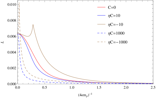
Figure 1: The luminosity $L$ of a 2D black hole against $(4\kappa m_{p})^{-1}$ with $\alpha=0.9$.

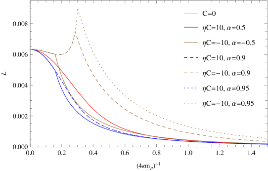
Figure 2: The luminosity $L$ of a 2D black hole against $\left(4\kappa m_{p}\right)^{-1}$ with $a=0.5,$ $0.9$ and $0.95$.

VII Discussion and Conclusion

In this paper, we used the Hamilton-Jacobi method to investigate the effects of the MDR on the Hawking radiation. Our results suggest that the thermal spectrum of radiations near horizon is robust. In fact, if the difference between the modified dispersion relation and the relativistic one was suppressed by the fundamental energy scale $m_{p},$ we found that the deviation of the effective Hawking temperature from the standard one was also suppressed by $m_{p}$. For a particle with the typical energy $\omega\sim\frac{m_{p}^{2}}{M}$, the deviation was given by powers of $\frac{m_{p}^{2}}{M^{2}}$. Nevertheless, there are some potential corrections to the effective Hawking temperature which are not included in our calculations:

1. Back-reaction effects which occurs at order $\frac{\omega}{M}$. For a particle with $\omega\sim\frac{m_{p}^{2}}{M}$, they are order of $\frac{m_{p}^{2}}{M^{2}}$. However, the Hamilton-Jacobi method is incapable of computing them since the metric is fixed in this method. On the other hand, back-reaction appears in the null geodesic method IN-Kraus:1994by ; IN-Kraus:1994fj to ensure energy conservation during the emission of a particle via tunneling through the horizon. These corrections lead to non-thermal corrections to the black-hole radiation spectrum. Note that there are some attempts to incorporate back-reaction effects into the Hamilton-Jacobi method using the rainbow metric CON-Medved:2005yf ; CON-Ding:2013bz .

2. Higher order WKB corrections. In the Hamilton-Jacobi method, we take the semi-classical limit $\hbar\rightarrow 0$ and keep only leading order terms to calculate the Hawking temperature. Therefore, one may wonder if the Hawking temperature could receive higher order corrections in $\hbar$ beyond the semiclassical one. The corrections has been estimated in CON-Banerjee:2008cf and was given by powers of $\frac{m_{p}^{2}}{M^{2}}$. However for the usual case, several authors CON-Yale:2010tn ; CON-Chatterjee:2009mw ; CON-Wang:2009zzw argued that the tunneling method yielded no higher-order corrections to the Hawking temperature. Whether such arguments also work for the MDR cases needs to be checked.

In this paper, we first used the Hamilton-Jacobi method to calculate tunneling rates of radiations across the horizon and the effective Hawking temperatures. After the spectrum of radiations near the horizon was obtained, the thermal entropy of radiations near the horizon and the luminosity of the black hole were computed. Our main results are as follows:

• In section II and the appendix, we used heuristic arguments and effective field theories, respectively to derive the deformed Hamilton-Jacobi equations incorporate the MDR with the static preferred frame. Note that these methods can easily be generalized to any preferred frame.

• In section II, the deformed Hamilton-Jacobi equations was solved for $\partial_{r}I$, and the imaginary part of $I$ was obtained by computing the residue of $\partial_{r}I$ at $r=r_{h}$. The assumption for our calculation was also discussed, which required that the singularity structure of $\partial_{r}I$ except the order of the pole at $r=r_{h}$ do not change after the MDR was introduced. The corrections to the Hawking temperature were calculated for massive and charged particles to $\mathcal{O}\left(m_{p}^{-2}\right)$ and neutral and massless particles to all orders, respectively. It was found that corrections were suppressed by $m_{p}$.

• In section IV, the average number and entropy for a mode were calculated for bosons and fermions. They could be obtained from those in the usual case by replacing the standard Hawking temperature with the modified one.

• In section V, we used the brick wall model to compute the thermal entropy of a massless scalar field near the horizon in UV finite and perturbative cases. In the UV finite case, the entropy was always finite as one approached the horizon, and hence the wall near the horizon was not needed. In the perturbative case, a wall was put at $r=r_{h}+r_{\varepsilon}$ to regulate the UV divergence. We assumed the proper distance between the horizon and the wall was order of $m_{p}$. Thus, the entropies near the horizon in both cases were given in eqn. $\left(\ref{eq:Entropy-MDR}\right)$. We found that the subleading logarithmic term of the entropy was independent of the MDR.

• In section VI, we calculated luminosities of a 4D spherically symmetric black hole with the mass $M\gg m_{p}$ and a 2D one. We used the geometric optics approximation to estimate the effects of scattering off the background.

Finally, we briefly discuss the results in this paper and IN-Wang . In this paper and IN-Wang , we have calculated the divergent part of the near horizon atmosphere entropy of a massless scalar field for a 4D spherically symmetric black hole in the static and free-fall scenarios, respectively. It appeared that the divergent part in both scenarios could be presented in the form of a Laurent series with respect to $r_{\varepsilon}$:

$$S\sim\frac{s_{1}^{0}}{\kappa r_{\varepsilon}}+s_{0}^{0}\ln\kappa r_{\varepsilon}+{\displaystyle\sum\limits_{i=1}^{\infty}}\frac{T_{0}^{2i}}{m_{p}^{2i}}\left({\displaystyle\sum\limits_{j=1}^{\delta_{i}}}s_{j}^{i}\left(\kappa r_{\varepsilon}\right)^{-j}+s_{0}^{i}\ln\kappa r_{\varepsilon}\right),$$ (151)

where $\delta_{i}=2i+1$ in the static scenario while $\delta_{i}=3i+1$ in the free-fall scenario.

Assuming the MDR for massless particles is

$$E^{2}=p{\displaystyle\sum\limits_{n=0}}\tilde{C}_{n}\frac{p^{2n}}{m_{p}^{2n}},$$ (152)

we found for the emission of $n_{s}$ species of massless scalars and $n_{f}$ species of massless spin-$1/2$ fermions that the total luminosity of a 4D Schwarzschild black hole was

$$L=\frac{9m_{p}^{2}}{40960M^{2}}\left[\left(n_{s}+\frac{7}{4}n_{f}\right)-\tilde{C}_{1}\left(0.73n_{s}+1.41n_{f}\right)\frac{m_{p}^{2}}{M^{2}}+\mathcal{O}\left(\frac{m_{p}^{3}}{M^{3}}\right)\right]\text{ in free-fall frame,}$$ (153)

$$L=\frac{9m_{p}^{2}}{40960\pi M^{2}}\left[\left(n_{s}+\frac{7}{4}n_{f}\right)+\tilde{C}_{1}\left(0.48n_{s}+0.92n_{f}\right)\frac{m_{p}^{2}}{M^{2}}+\mathcal{O}\left(\frac{m_{p}^{3}}{M^{3}}\right)\right]\text{ in static frame.}$$ (154)

Note that the sign in front of $\tilde{C}_{1}$ in eqn. $\left(\ref{eq:L-ff}\right)$ is different from that in eqn. $\left(\ref{eq:L-sf}\right).$ For the sub-luminal dispersion relation with $\tilde{C}_{1}<0$, it means that the total luminosity increases due to the MDR effects in the free-fall scenario while it decreases in the static scenario.

Appendix A Effective Field Theory and Deformed Hamilton-Jacobi Equation

As discussed in the introduction, various approaches to the quantum-gravity problem could lead to the existence of MDRs. To have a MDR, one has to break or modify the global Lorentz symmetry in the classical limit of the quantum gravity. There are several possibilities for breaking or modifying the Lorentz symmetry, one of which is that Lorentz invariance is spontaneously broken by extra tensor fields taking on vacuum expectation values. The most conservative approach for a framework in which to describe MDR is the effective field theory (EFT), where modifications to the dispersion relation can be described by the higher dimensional operators. Since we are only interested in modifications to the dispersion relation of the particles, we limit ourselves to the kinetic terms and neglect self-interacting effective operators when constructing the effective field theory. We also assume that the effective theory respects $U\left(1\right)$ gauge invariance of the charged black hole. The EFT framework can easily incorporate MDR via the introduction of extra tensors. To construct the minimal EFT in curved spacetime, we suppose that the action of the EFT contains the usual minimal gravitational couplings and the EFT coefficients are constants in the local frameAPD-Kostelecky:2003fs .

A.1 Scalar Field

We work with a complex scalar field $\phi$ with the mass $m$ and the charge $q$. Following guidelines we put forth, we find the effective Lagrangian for $\phi$ incorporating MDR can be written as

$$\mathcal{L}_{eff}^{s} =-\phi^{+}\left(D^{\mu}D_{\mu}+\frac{m^{2}}{\hbar^{2}}\right)\phi-\frac{m^{2}B\left(\frac{m}{m_{p}}\right)}{\hbar^{2}}\phi^{+}\phi-\frac{imC_{\mu}\left(\frac{m}{m_{p}}\right)}{\hbar}\phi^{+}D^{\mu}\phi$$

$$-{\displaystyle\sum\limits_{n\geq 2,j}}\left(\frac{\hbar}{i}\right)^{n-2}\frac{C_{\mu_{1}\cdots\mu_{n}}^{j}\left(\frac{m}{m_{p}}\right)}{m_{p}^{n-2}}\phi^{+}D^{\mu_{1}}\cdots D^{\mu_{n}}\phi,$$ (155)

where $D_{\mu}=\nabla_{\mu}+\frac{iq}{\hbar}A_{\mu},$ $\nabla_{\mu}$ is the covariant derivative of the background spacetime, $A_{\mu\text{ }}$is the electromagnetic potential, $j$ runs over all independent operators of a given dimension, $B$ is a dimensionless function of $\frac{m}{m_{p}}$ with $B\left(0\right)=0$, and, $C_{\mu}$ and $C_{\mu_{1}\cdots\mu_{n}}^{j}$ are dimensionless extra tensors depending on $\frac{m}{m_{p}}$ with $C_{\mu}\left(0\right)=C_{\mu\nu}^{j}\left(0\right)=0.$ The deformed Klein-Gordon equation is

$$-\left(D^{\mu}D_{\mu}+\frac{m^{2}}{\hbar^{2}}\right)\phi-\frac{m^{2}B\left(\frac{m}{m_{p}}\right)}{\hbar^{2}}\phi-\frac{imC_{\mu}\left(\frac{m}{m_{p}}\right)}{\hbar}D^{\mu}\phi$$

$$-{\displaystyle\sum\limits_{n\geq 2,j}}\left(\frac{\hbar}{i}\right)^{n-2}\frac{C_{\mu_{1}\cdots\mu_{n}}^{j}\left(\frac{m}{m_{p}}\right)}{m_{p}^{n-2}}D^{\mu_{1}}\cdots D^{\mu_{n}}\phi=0.$$ (156)

With rotational symmetry, all extra tensors become reducible to products of a vector field $u^{\mu}$, which describes the preferred frame and $u^{\mu}u_{\mu}=1$. Thus, the extra tensors become

$$C_{\mu} =C\left(\frac{m}{m_{p}}\right)u^{\mu},$$

$$C_{\mu_{1}\cdots\mu_{n}}^{j} =C_{n}^{j}\left(\frac{m}{m_{p}}\right)g_{\mu_{i_{1}}\mu_{i_{2}}}\cdots g_{\mu_{i_{2k-1}}\mu_{i_{2k}}}u_{\mu_{i_{2k+1}}}\cdots u_{\mu_{i_{n}}},$$ (157)

where $g_{\mu\nu}$ is the metric of the background spacetime, $C$ and $C_{n}^{j}$ are dimensionless functions of $\frac{m}{m_{p}},$ $j=\left(k,\mathcal{C}\right),$ $2k\leq n,$ and $\mathcal{C}$ denotes any possible permutations of $\left(1,\cdots,n\right)$, namely $\left(i_{1},\cdots,i_{n}\right)$. To obtain the Hamilton-Jacobi equation, we make the WKB ansatz for $\phi$

$$\phi=\exp\left(\frac{iI}{\hbar}\right).$$ (158)

Defining

$$\tilde{T}=-u^{\mu}\left(\partial_{\mu}I+qA_{\mu}\right),\text{ }\tilde{X}^{2}=\tilde{T}^{2}-\left(\partial_{\mu}I+qA_{\mu}\right)^{2},$$ (159)

and plugging eqns. $\left(\ref{eq:ansatzS}\right)$ and $\left(\ref{eq:cnj-coef}\right)$ into eqn. $\left(\ref{eq:DeformedKG}\right)$, one expands eqn. $\left(\ref{eq:DeformedKG}\right)$ in powers of $\hbar$ and finds to the lowest order

$$\left(\tilde{T}^{2}-\tilde{X}^{2}-m^{2}\right)-m^{2}B\left(\frac{m}{m_{p}}\right)-mC\left(\frac{m}{m_{p}}\right)\tilde{T}+{\displaystyle\sum\limits_{n\geq 2,k\leq\frac{n}{2},\mathcal{C}}}\frac{\left(-1\right)^{n}C_{n}^{j}\left(\frac{m}{m_{p}}\right)\left(\tilde{T}^{2}-\tilde{X}^{2}\right)^{k}\tilde{T}^{n-2k}}{m_{p}^{n-2}}=0.$$ (160)

Solving eqn. $\left(\ref{eq:deformedHJS}\right)$ for $\tilde{X}^{2}$ with respect to $\tilde{T}$ gives the deformed Hamilton-Jacobi equation for $I$

$$\tilde{X}^{2}=\alpha\left(\frac{m}{m_{p}}\right)\tilde{T}^{2}-\beta\left(\frac{m}{m_{p}}\right)m^{2}+\gamma\left(\frac{m}{m_{p}}\right)m\tilde{T}+\sum_{n\geq 3}\frac{C_{n}\left(\frac{m}{m_{p}}\right)\tilde{T}^{n}}{m_{p}^{n-2}},$$ (161)

where $\alpha,\beta,\gamma$ are dimensionless functions of $\frac{m}{m_{p}}$ with $\alpha\left(0\right)=\beta\left(0\right)=1$ and $\gamma\left(0\right)=0$ which can be determined by the coefficients $B$, $C$ and $C_{n}^{j}$ in eqn. $\left(\ref{eq:deformedHJS}\right)$. In flat spacetime with $A_{\mu}=0$, the dispersion relation for the scalar field can be found by inserting the positive energy ansatz $\phi=\exp\left(-\frac{ip_{\mu}x^{\mu}}{\hbar}\right)$ into eqn. $\left(\ref{eq:DeformedKG}\right)$. The resulting equation for $p_{\mu}$ is actually eqn. $\left(\ref{eq:deformedHJSS}\right)$ with $\tilde{T}=u^{\mu}p_{\mu}$ and $\tilde{X}^{2}=-p_{\mu}p^{\mu}+\tilde{T}^{2}$, which is exact for flat spacetime with $A_{\mu}=0$. Identifying $E=p_{\mu}u^{\mu}=\tilde{T}$ and $p^{2}=-p_{\mu}^{\left(3\right)}p^{\left(3\right),\mu}=-p_{\mu}p^{\mu}+\tilde{T}^{2}=\tilde{X}^{2}$, we can produce the MDR for the scalar, eqn. $\left(\ref{eq:MDRExpansion}\right),$ in flat spacetime. On the other hand, the vector field $u^{\mu}$ is chosen to be $\left(\frac{1}{\sqrt{f\left(r\right)}},\vec{0}\right)$ in curved spacetime with the metric $\left(\ref{eq:BHmetric}\right)$ and the electromagnetic potential $A_{\mu}$. In this case, $\tilde{T}$ and $\tilde{X}^{2}$ become $T$ and $X^{2}$ in eqn. $\left(\ref{eq:TandX}\right)$. Thus, in the black hole background spacetime, the corresponding deformed Hamilton-Jacobi equation for the scalar field incorporating the MDR, eqn. $\left(\ref{eq:MDRExpansion}\right),$ is given by eqn. $\left(\ref{eq:deformedHJeqn}\right).$

A.2 Fermionic Field

In the background spacetime with the metric $g_{\mu\nu}$ and the electromagnetic potential $A_{\mu}$, the effective Lagrangian for a spin-$1/2$ fermion $\psi$ with the mass $m$ and the charge $q$ incorporating the MDR can be written as

$$\mathcal{L}_{eff}^{f}=\bar{\psi}\left(iD_{\mu}^{f}\gamma^{\mu}-\frac{m}{\hbar}\right)\psi-\frac{m}{\hbar}{\displaystyle\sum\limits_{k\geq 0,j}}B_{\mu_{1}\cdots\mu_{k}}^{j}\left(\frac{m}{m_{p}}\right)\bar{\psi}\gamma^{\mu_{1}}\cdots\gamma^{\mu_{k}}\psi$$

$$+i{\displaystyle\sum\limits_{n\geq k\geq 1,j}}\left(\frac{\hbar}{i}\right)^{k-1}\frac{C_{\mu_{1}\cdots\mu_{n}}^{j}\left(\frac{m}{m_{p}}\right)}{m_{p}^{k-1}}\bar{\psi}D^{f,\mu_{1}}\cdots D^{f,\mu_{k}}\gamma^{\mu_{k+1}}\cdots\gamma^{\mu_{n}}\psi,$$ (162)

where extra tensors $B_{\mu_{1}\cdots\mu_{k}}^{j}$ and $C_{\mu_{1}\cdots\mu_{n}}^{j}$ are dimensionless functions of $\frac{m}{m_{p}}$ with $B_{\mu_{1}\cdots\mu_{k}}^{j}\left(0\right)=C_{\mu}^{j}\left(0\right)=0$, $j$ runs over all independent operators of a given dimension, $D_{\mu}^{f}=\partial_{\mu}+\Omega_{\mu}+\frac{iq}{\hbar}A_{\mu}$, $\Omega_{\mu}\equiv\frac{i}{2}\omega_{\mu}^{\text{ }ab}\Sigma_{ab}$, $\Sigma_{ab}$ is the Lorentz spinor generator, $\omega_{\mu}^{\text{ }ab}$ is the spin connection and $\left\{\gamma_{\mu},\gamma_{\nu}\right\}=2g_{\mu\nu}$. The Greek indices are raised and lowered by the curved metric $g_{\mu\nu}$, while the Latin indices are governed by the flat metric $\eta_{ab}$. The deformed Dirac equation is

$$\left(iD_{\mu}^{f}\gamma^{\mu}-\frac{m}{\hbar}\right)\psi-\frac{m}{\hbar}{\displaystyle\sum\limits_{n\geq 0,j}}B_{\mu_{1}\cdots\mu_{n}}^{j}\left(\frac{m}{m_{p}}\right)\gamma^{\mu_{1}}\cdots\gamma^{\mu_{n}}\psi$$

$$+i{\displaystyle\sum\limits_{n\geq k\geq 1,j}}\left(\frac{\hbar}{i}\right)^{m-1}\frac{C_{\mu_{1}\cdots\mu_{n}}^{j}\left(\frac{m}{m_{p}}\right)}{m_{p}^{k-1}}D^{f,\mu_{1}}\cdots D^{f,\mu_{k}}\gamma^{\mu_{k+1}}\cdots\gamma^{\mu_{n}}\psi=0.$$ (163)

With rotational symmetry, the extra tensors become

$$B_{\mu_{1}\cdots\mu_{n}}^{j} =B_{n}^{j}g_{\mu_{i_{1}}\mu_{i_{2}}}\cdots g_{\mu_{i_{2k-1}}\mu_{i_{2k}}}u_{\mu_{i_{2k+1}}}\cdots u_{\mu_{i_{n}}},$$

$$C_{\mu_{1}\cdots\mu_{n}}^{j} =C_{n}^{j}g_{\mu_{i_{1}}\mu_{i_{2}}}\cdots g_{\mu_{i_{2k-1}}\mu_{i_{2k}}}u_{\mu_{i_{2k+1}}}\cdots u_{\mu_{i_{n}}},$$ (164)

where $B_{n}^{j}$ and $C_{n}^{j}$ are dimensionless functions of $\frac{m}{m_{p}},$ $j=\left(k,\mathcal{C}\right),$ $2k\leq n,$ and $\mathcal{C}$ denotes any possible permutations of $\left(1,\cdots,n\right)$, namely $\left(i_{1},\cdots,i_{n}\right)$. To obtain the deformed Hamilton-Jacobi equation, the ansatz for $\psi$ is assumed as

$$\psi=\exp\left(\frac{iI}{\hbar}\right)\mathbf{v},$$ (165)

where $\mathbf{v}$ is a slowly varying spinor amplitude. Substituting eqn. $\left(\ref{eq:fermionansatz}\right)$ into eqn. $\left(\ref{eq:deformedDirac}\right)$, we find to the lowest order of $\hbar$

$$X_{\mu}\gamma^{\mu}\mathbf{v}+m\mathbf{v}+m{\displaystyle\sum\limits_{n\geq 0,k\leq\frac{n}{2},\mathcal{C}}}B_{n}^{j}g_{\mu_{i_{1}}\mu_{i_{2}}}\cdots g_{\mu_{i_{2k-1}}\mu_{i_{2k}}}u_{\mu_{i_{2k+1}}}\cdots u_{\mu_{i_{n}}}\gamma^{\mu_{1}}\cdots\gamma^{\mu_{n}}\mathbf{v}$$

$$+{\displaystyle\sum\limits_{n\geq k\geq 1,l\leq\frac{n}{2},\mathcal{C}}}\frac{C_{n}^{j}}{m_{p}^{k-1}}g_{\mu_{i_{1}}\mu_{i_{2}}}\cdots g_{\mu_{i_{2l-1}}\mu_{i_{2l}}}u_{\mu_{i_{2l+1}}}\cdots u_{\mu_{i_{n}}}X^{\mu_{1}}\cdots X^{\mu_{k}}\gamma^{\mu_{k+1}}\cdots\gamma^{\mu_{n}}\mathbf{v}=0,$$ (166)

where $X_{\mu}=\partial_{\mu}I+qA_{\mu}$. Using $\left(X_{\mu}\gamma^{\mu}\right)^{2}=\left(X_{\mu}\right)^{2}=\tilde{T}^{2}-\tilde{X}^{2}$, $\left(u_{\mu}\gamma^{\mu}\right)\left(X_{\mu}\gamma^{\mu}\right)=u_{\mu}X^{\mu}=-\tilde{T}$, and $\left(u_{\mu}\gamma^{\mu}\right)^{2}=1,$ one could rewrite eqn. $\left(\ref{eq:deformedHJF}\right)$ as

$$\left[X_{\mu}+mC_{1}\left(\frac{m}{m_{p}}\right)u_{\mu}+h_{2}\left(\tilde{T},\tilde{X}^{2}\right)u_{\mu}+g\left(\tilde{T},\tilde{X}^{2}\right)X_{\mu}\right]\gamma^{\mu}\mathbf{v}=-\left[m+mC_{2}\left(\frac{m}{m_{p}}\right)+h_{1}\left(\tilde{T},\tilde{X}^{2}\right)\right]\mathbf{v,}$$ (167)

where $C_{i}$ are dimensionless functions of $\frac{m}{m_{p}}$ with $C_{i}\left(0\right)=0$, $h_{i}\left(\tilde{T},\tilde{X}^{2}\right)={\displaystyle\sum\limits_{2p+q\geq 1}}\frac{h_{i}^{p,q}\left(\frac{m}{m_{p}}\right)\tilde{T}^{q}\left(\tilde{T}^{2}-\tilde{X}^{2}\right)^{p}}{m_{p}^{2p+q-1}}$ and $g_{i}\left(\tilde{T},\tilde{X}^{2}\right)={\displaystyle\sum\limits_{2p+q\geq 0}}\frac{g^{p,q}\left(\frac{m}{m_{p}}\right)\tilde{T}^{q}\left(\tilde{T}^{2}-\tilde{X}^{2}\right)^{p}}{m_{p}^{2p+q}}$. The coefficients $C_{i}$, $h_{i}^{p,q}$ and $g^{p,q}$ are determined by $B_{n}^{j}$ and $C_{n}^{j}$ from eqn. $\left(\ref{eq:deformedHJF}\right)$. However, the detailed relations between them are irrelevant here. Multiplying both sides of eqn. $\left(\ref{eq:deformedHJFF}\right)$ from the left by $\left(X_{\mu}+mC_{1}u_{\mu}+h_{2}u_{\mu}+gX_{\mu}\right)\gamma^{\mu}\,$and then using eqn. $\left(\ref{eq:deformedHJFF}\right)$ and $\left\{\gamma_{\mu},\gamma_{\nu}\right\}=2g_{\mu\nu}$ to simplify the RHS, one gets

$$\left(X^{\mu}+mC_{1}u^{\mu}+h_{2}u^{\mu}+gX^{\mu}\right)\left(X_{\mu}+mC_{1}u_{\mu}+h_{2}u_{\mu}+gX_{\mu}\right)\mathbf{v}=\left(m+mC_{2}+h_{1}\right)^{2}\mathbf{v}.$$ (168)

Since $\mathbf{v}$ is nonzero, eqn. $\left(\ref{eq:deformedHJFFF}\right)$ gives

$$\left(\tilde{T}^{2}-\tilde{X}^{2}-m^{2}\right)-m^{2}B\left(\frac{m}{m_{p}}\right)-mC\left(\frac{m}{m_{p}}\right)\tilde{T}+{\displaystyle\sum\limits_{n\geq 2,k\leq\frac{n}{2},\mathcal{C}}}\frac{C_{n}^{j}\left(\frac{m}{m_{p}}\right)\left(\tilde{T}^{2}-\tilde{X}^{2}\right)^{k}\tilde{T}^{n-2k}}{m_{p}^{n-2}}=0,$$ (169)

where

$$B=-C_{1}^{2}+C_{2}^{2}+2C_{2},$$

$$C=2C_{1}+2g^{0,0}C_{1}+2C_{1}h_{2}^{0,1}-2\left(1+C_{2}\right)h_{1}^{0,1},$$

$${\displaystyle\sum}\frac{C_{n}^{j}\left(\tilde{T}^{2}-\tilde{X}^{2}\right)^{k}\tilde{T}^{n-2k}}{m_{p}^{n-2}}=g\left(\tilde{T}^{2}-\tilde{X}^{2}\right)+2\left(h_{2}+gh_{2}\right)\tilde{T}-h_{1}^{2}+h_{2}^{2}$$

$$+2m\left(g-g^{0,0}\right)C_{1}\tilde{T}+2mC_{1}\left(h_{2}-h_{2}^{0,1}\tilde{T}\right)-2m\left(1+C_{2}\right)\left(h_{1}-h_{1}^{0,1}\tilde{T}\right).$$

It is noted that the form of eqn. $\left(\ref{eq:deformedHJFFF}\right)$ is the same as that of eqn. $\left(\ref{eq:deformedHJS}\right)$. Thus, the argument and result below eqn. $\left(\ref{eq:deformedHJSS}\right)$ can also apply to a spin-$1/2$ fermion field.

References

- (1) S. W. Hawking, “Particle Creation by Black Holes,” Commun. Math. Phys. 43, 199 (1975) [Erratum-ibid. 46, 206 (1976)].
- (2) W. G. Unruh, “Notes on black hole evaporation,” Phys. Rev. D 14, 870 (1976).
- (3) S. Weinberg, “What is quantum field theory, and what did we think it is?,” In *Boston 1996, Conceptual foundations of quantum field theory* 241-251 [hep-th/9702027].
- (4) G. Amelino-Camelia, “Introduction to quantum-gravity phenomenology,” Lect. Notes Phys. 669, 59 (2005) [gr-qc/0412136].
- (5) G. Amelino-Camelia, J. R. Ellis, N. E. Mavromatos, D. V. Nanopoulos and S. Sarkar, “Tests of quantum gravity from observations of gamma-ray bursts,” Nature 393, 763 (1998) [astro-ph/9712103].
- (6) L. J. Garay, “Space-time foam as a quantum thermal bath,” Phys. Rev. Lett. 80, 2508 (1998) [gr-qc/9801024].
- (7) G. Amelino-Camelia, “Doubly special relativity,” Nature 418, 34 (2002) [gr-qc/0207049].
- (8) J. Magueijo and L. Smolin, “Generalized Lorentz invariance with an invariant energy scale,” Phys. Rev. D 67, 044017 (2003) [gr-qc/0207085].
- (9) D. Mattingly, “Modern tests of Lorentz invariance,” Living Rev. Rel. 8, 5 (2005) [gr-qc/0502097].
- (10) S. Liberati, “Tests of Lorentz invariance: a 2013 update,” Class. Quant. Grav. 30, 133001 (2013) [arXiv:1304.5795 [gr-qc]].
- (11) D. Colladay and V. A. Kostelecky, “Lorentz violating extension of the standard model,” Phys. Rev. D 58, 116002 (1998) [hep-ph/9809521].
- (12) S. R. Coleman and S. L. Glashow, “High-energy tests of Lorentz invariance,” Phys. Rev. D 59, 116008 (1999) [hep-ph/9812418].
- (13) G. Amelino-Camelia and T. Piran, “Planck scale deformation of Lorentz symmetry as a solution to the UHECR and the TeV gamma paradoxes,” Phys. Rev. D 64, 036005 (2001) [astro-ph/0008107].
- (14) T. Jacobson, S. Liberati and D. Mattingly, “TeV astrophysics constraints on Planck scale Lorentz violation,” Phys. Rev. D 66, 081302 (2002) [hep-ph/0112207].
- (15) T. A. Jacobson, S. Liberati, D. Mattingly and F. W. Stecker, “New limits on Planck scale Lorentz violation in QED,” Phys. Rev. Lett. 93, 021101 (2004) [astro-ph/0309681].
- (16) G. Amelino-Camelia, M. Arzano and A. Procaccini, “Severe constraints on loop-quantum-gravity energy-momentum dispersion relation from black-hole area-entropy law,” Phys. Rev. D 70, 107501 (2004) [gr-qc/0405084].
- (17) Y. Ling, B. Hu and X. Li, “Modified dispersion relations and black hole physics,” Phys. Rev. D 73, 087702 (2006) [gr-qc/0512083].
- (18) G. Amelino-Camelia, M. Arzano, Y. Ling and G. Mandanici, “Black-hole thermodynamics with modified dispersion relations and generalized uncertainty principles,” Class. Quant. Grav. 23, 2585 (2006) [gr-qc/0506110].
- (19) K. Nozari and A. S. Sefiedgar, “Comparison of approaches to quantum correction of black hole thermodynamics,” Phys. Lett. B 635 (2006) 156 [gr-qc/0601116].
- (20) A. S. Sefiedgar, K. Nozari and H. R. Sepangi, “Modified dispersion relations in extra dimensions,” Phys. Lett. B 696, 119 (2011) [arXiv:1012.1406 [gr-qc]].
- (21) B. Majumder, “Black Hole Entropy and the Modified Uncertainty Principle: A heuristic analysis,” Phys. Lett. B 703, 402 (2011) [arXiv:1106.0715 [gr-qc]].
- (22) P. Kraus and F. Wilczek, “Selfinteraction correction to black hole radiance,” Nucl. Phys. B 433, 403 (1995) [gr-qc/9408003].
- (23) P. Kraus and F. Wilczek, “Effect of selfinteraction on charged black hole radiance,” Nucl. Phys. B 437, 231 (1995) [hep-th/9411219].
- (24) K. Srinivasan and T. Padmanabhan, “Particle production and complex path analysis,” Phys. Rev. D 60, 024007 (1999) [gr-qc/9812028].
- (25) M. Angheben, M. Nadalini, L. Vanzo and S. Zerbini, “Hawking radiation as tunneling for extremal and rotating black holes,” JHEP 0505, 014 (2005) [hep-th/0503081].
- (26) R. Kerner and R. B. Mann, “Tunnelling, temperature and Taub-NUT black holes,” Phys. Rev. D 73, 104010 (2006) [gr-qc/0603019].
- (27) S. Hemming and E. Keski-Vakkuri, “The Spectrum of strings on BTZ black holes and spectral flow in the SL(2,R) WZW model,” Nucl. Phys. B 626, 363 (2002) [hep-th/0110252].
- (28) A. J. M. Medved, “Radiation via tunneling from a de Sitter cosmological horizon,” Phys. Rev. D 66, 124009 (2002) [hep-th/0207247].
- (29) E. C. Vagenas, “Semiclassical corrections to the Bekenstein-Hawking entropy of the BTZ black hole via selfgravitation,” Phys. Lett. B 533, 302 (2002) [hep-th/0109108].
- (30) M. Arzano, A. J. M. Medved and E. C. Vagenas, “Hawking radiation as tunneling through the quantum horizon,” JHEP 0509, 037 (2005) [hep-th/0505266].
- (31) S. Q. Wu and Q. Q. Jiang, “Remarks on Hawking radiation as tunneling from the BTZ black holes,” JHEP 0603, 079 (2006) [hep-th/0602033].
- (32) M. Nadalini, L. Vanzo and S. Zerbini, “Hawking radiation as tunneling: The D dimensional rotating case,” J. Phys. A 39, 6601 (2006) [hep-th/0511250].
- (33) B. Chatterjee, A. Ghosh and P. Mitra, “Tunnelling from black holes in the Hamilton Jacobi approach,” Phys. Lett. B 661, 307 (2008) [arXiv:0704.1746 [hep-th]].
- (34) V. Akhmedova, T. Pilling, A. de Gill and D. Singleton, “Temporal contribution to gravitational WKB-like calculations,” Phys. Lett. B 666, 269 (2008) [arXiv:0804.2289 [hep-th]].
- (35) E. T. Akhmedov, T. Pilling and D. Singleton, “Subtleties in the quasi-classical calculation of Hawking radiation,” Int. J. Mod. Phys. D 17, 2453 (2008) [arXiv:0805.2653 [gr-qc]].
- (36) V. Akhmedova, T. Pilling, A. de Gill and D. Singleton, “Comments on anomaly versus WKB/tunneling methods for calculating Unruh radiation,” Phys. Lett. B 673, 227 (2009) [arXiv:0808.3413 [hep-th]].
- (37) R. Banerjee and B. R. Majhi, “Quantum Tunneling and Back Reaction,” Phys. Lett. B 662, 62 (2008) [arXiv:0801.0200 [hep-th]].
- (38) D. Singleton, E. C. Vagenas, T. Zhu and J. R. Ren, “Insights and possible resolution to the information loss paradox via the tunneling picture,” JHEP 1008, 089 (2010) [Erratum-ibid. 1101, 021 (2011)] [arXiv:1005.3778 [gr-qc]].
- (39) D. Chen, H. Wu and H. Yang, “Fermion’s tunnelling with effects of quantum gravity,” Adv. High Energy Phys. 2013, 432412 (2013) [arXiv:1305.7104 [gr-qc]].
- (40) D. Chen, H. Wu and H. Yang, “Observing remnants by fermions’ tunneling,” JCAP 1403, 036 (2014) [arXiv:1307.0172 [gr-qc]].
- (41) D. Y. Chen, Q. Q. Jiang, P. Wang and H. Yang, “Remnants, fermions‘ tunnelling and effects of quantum gravity,” JHEP 1311, 176 (2013) [arXiv:1312.3781 [hep-th]].
- (42) D. Chen and Z. Li, “Remarks on Remnants by Fermions’ Tunnelling from Black Strings,” Adv. High Energy Phys. 2014, 620157 (2014) [arXiv:1404.6375 [hep-th]].
- (43) D. Chen, H. Wu, H. Yang and S. Yang, Int. J. Mod. Phys. A 29, no. 26, 1430054 (2014) [arXiv:1410.5071 [gr-qc]].
- (44) B. Mu, P. Wang and H. Yang, “Minimal Length Effects on Tunnelling from Spherically Symmetric Black Holes,” Adv. High Energy Phys. 2015, 898916 (2015) [arXiv:1501.06025 [gr-qc]].
- (45) P. Wang, H. Yang and S. Ying, “Black Hole Radiation with Modified Dispersion Relation in Tunneling Paradigm: Free-fall Frame,” Eur. Phys. J. C 76, no. 1, 27 (2016) [arXiv:1505.04568 [gr-qc]].
- (46) J. D. Bekenstein, “Black holes and entropy,” Phys. Rev. D 7, 2333 (1973).
- (47) W. G. Unruh, “Sonic analog of black holes and the effects of high frequencies on black hole evaporation,” Phys. Rev. D 51, 2827 (1995).
- (48) R. Brout, S. Massar, R. Parentani and P. Spindel, “Hawking radiation without transPlanckian frequencies,” Phys. Rev. D 52, 4559 (1995) [hep-th/9506121].
- (49) S. Corley and T. Jacobson, “Hawking spectrum and high frequency dispersion,” Phys. Rev. D 54, 1568 (1996) [hep-th/9601073].
- (50) S. Corley, “Computing the spectrum of black hole radiation in the presence of high frequency dispersion: An Analytical approach,” Phys. Rev. D 57, 6280 (1998) [hep-th/9710075].
- (51) Y. Himemoto and T. Tanaka, “A Generalization of the model of Hawking radiation with modified high frequency dispersion relation,” Phys. Rev. D 61, 064004 (2000) [gr-qc/9904076].
- (52) H. Saida and M. a. Sakagami, “Black hole radiation with high frequency dispersion,” Phys. Rev. D 61, 084023 (2000) [gr-qc/9905034].
- (53) W. G. Unruh and R. Schutzhold, “On the universality of the Hawking effect,” Phys. Rev. D 71, 024028 (2005) [gr-qc/0408009].
- (54) J. Macher and R. Parentani, “Black/White hole radiation from dispersive theories,” Phys. Rev. D 79, 124008 (2009) [arXiv:0903.2224 [hep-th]].
- (55) A. Coutant, R. Parentani and S. Finazzi, “Black hole radiation with short distance dispersion, an analytical S-matrix approach,” Phys. Rev. D 85, 024021 (2012) [arXiv:1108.1821 [hep-th]].
- (56) A. Coutant and R. Parentani, “Hawking radiation with dispersion: The broadened horizon paradigm,” Phys. Rev. D 90, no. 12, 121501 (2014) [arXiv:1402.2514 [gr-qc]].
- (57) F. Belgiorno, S. L. Cacciatori and F. D. Piazza, “Tunneling approach and thermality in dispersive models of analogue gravity,” arXiv:1411.7871 [gr-qc].
- (58) D. Chang, C. S. Chu and F. L. Lin, “TransPlanckian entanglement entropy,” Phys. Lett. B 583, 192 (2004) [hep-th/0306055].
- (59) Y. W. Kim and Y. J. Park, “Entropy of the Schwarzschild black hole to all orders in the Planck length,” Phys. Lett. B 655, 172 (2007) [arXiv:0707.2128 [gr-qc]].
- (60) E. T. Akhmedov, V. Akhmedova and D. Singleton, “Hawking temperature in the tunneling picture,” Phys. Lett. B 642, 124 (2006) [hep-th/0608098].
- (61) P. Mitra, “Hawking temperature from tunnelling formalism,” Phys. Lett. B 648, 240 (2007) [hep-th/0611265].
- (62) V. Akhmedova, T. Pilling, A. de Gill and D. Singleton, “Comments on anomaly versus WKB/tunneling methods for calculating Unruh radiation,” Phys. Lett. B 673, 227 (2009) [arXiv:0808.3413 [hep-th]].
- (63) B. D. Chowdhury, “Problems with Tunneling of Thin Shells from Black Holes,” Pramana 70, 593 (2008) [Pramana 70, 3 (2008)] [hep-th/0605197].
- (64) V. Akhmedova, T. Pilling, A. de Gill and D. Singleton, “Temporal contribution to gravitational WKB-like calculations,” Phys. Lett. B 666, 269 (2008) [arXiv:0804.2289 [hep-th]].
- (65) A. de Gill, D. Singleton, V. Akhmedova and T. Pilling, “A WKB-Like Approach to Unruh Radiation,” Am. J. Phys. 78, 685 (2010) [arXiv:1001.4833 [gr-qc]].
- (66) L. Vanzo, G. Acquaviva and R. Di Criscienzo, “Tunnelling Methods and Hawking’s radiation: achievements and prospects,” Class. Quant. Grav. 28, 183001 (2011) [arXiv:1106.4153 [gr-qc]].
- (67) P. K. Townsend, “Small Scale Structure of Space-Time as the Origin of the Gravitational Constant,” Phys. Rev. D 15, 2795 (1977).
- (68) D. Amati, M. Ciafaloni and G. Veneziano, “Can Space-Time Be Probed Below the String Size?,” Phys. Lett. B 216, 41 (1989).
- (69) K. Konishi, G. Paffuti and P. Provero, “Minimum Physical Length and the Generalized Uncertainty Principle in String Theory,” Phys. Lett. B 234, 276 (1990).
- (70) A. Kempf, G. Mangano and R. B. Mann, “Hilbert space representation of the minimal length uncertainty relation,” Phys. Rev. D 52, 1108 (1995) [hep-th/9412167].
- (71) S. Hossenfelder, M. Bleicher, S. Hofmann, J. Ruppert, S. Scherer and H. Stoecker, “Collider signatures in the Planck regime,” Phys. Lett. B 575, 85 (2003) [hep-th/0305262].
- (72) J. B. Hartle and S. W. Hawking, “Path Integral Derivation of Black Hole Radiance,” Phys. Rev. D 13, 2188 (1976).
- (73) T. Appelquist and J. Carazzone, “Infrared Singularities and Massive Fields,” Phys. Rev. D 11, 2856 (1975).
- (74) G. ’t Hooft, “On the Quantum Structure of a Black Hole,” Nucl. Phys. B 256, 727 (1985).
- (75) J. Kowalski-Glikman and S. Nowak, “Noncommutative space-time of doubly special relativity theories,” Int. J. Mod. Phys. D 12, 299 (2003) [hep-th/0204245].
- (76) S. N. Solodukhin, “The Conical singularity and quantum corrections to entropy of black hole,” Phys. Rev. D 51, 609 (1995) [hep-th/9407001].
- (77) S. N. Solodukhin, “Entanglement entropy of black holes,” Living Rev. Rel. 14, 8 (2011) [arXiv:1104.3712 [hep-th]].
- (78) N. Iizuka and S. Terashima, “Brick Walls for Black Holes in AdS/CFT,” arXiv:1307.5933 [hep-th].
- (79) P. Wang, H. Yang and S. Ying, “Minimal Length Effects on Entanglement Entropy of Spherically Symmetric Black Holes in Brick Wall Model,” arXiv:1502.00204 [gr-qc].
- (80) D. N. Page, “Particle Emission Rates from a Black Hole: Massless Particles from an Uncharged, Nonrotating Hole,” Phys. Rev. D 13, 198 (1976).
- (81) T. Jacobson, “Lorentz violation and Hawking radiation,” gr-qc/0110079.
- (82) A. J. M. Medved and E. C. Vagenas, “On Hawking radiation as tunneling with back-reaction,” Mod. Phys. Lett. A 20, 2449 (2005) [gr-qc/0504113].
- (83) C. Ding, “Hawking radiation and total entropy change as tunneling,” Int. J. Theor. Phys. 53, 694 (2014) [arXiv:1302.0353 [gr-qc]].
- (84) R. Banerjee and B. R. Majhi, “Quantum Tunneling Beyond Semiclassical Approximation,” JHEP 0806, 095 (2008) [arXiv:0805.2220 [hep-th]].
- (85) A. Yale, “Exact Hawking Radiation of Scalars, Fermions, and Bosons Using the Tunneling Method Without Back-Reaction,” Phys. Lett. B 697, 398 (2011) [arXiv:1012.3165 [gr-qc]].
- (86) B. Chatterjee and P. Mitra, “Hawking temperature and higher order tunnelling calculations,” Phys. Lett. B 675, 240 (2009) [arXiv:0902.0230 [gr-qc]].
- (87) M. Wang, C. Ding, S. Chen and J. Jing, “Is Hawking temperature modified by the quantum tunneling beyond semiclassical approximation,” Gen. Rel. Grav. 42, 347 (2010).
- (88) V. A. Kostelecky, “Gravity, Lorentz violation, and the standard model,” Phys. Rev. D 69, 105009 (2004) [hep-th/0312310].