k²Q: A Quadratic-Form Response Time and Schedulability Analysis Framework for Utilization-Based Analysis

Abstract

In this paper, we present a general response-time analysis and schedulability-test framework, called $\mathbf{k^{2}Q}$ (k to Q). It provides automatic constructions of closed-form quadratic bounds or utilization bounds for a wide range of applications in real-time systems under fixed-priority scheduling. The key of the framework is a $k$-point schedulability test or a $k$-point response time analysis that is based on the utilizations and the execution times of $k-1$ higher-priority tasks. The natural condition of $\mathbf{k^{2}Q}$ is a quadratic form for testing the schedulability or analyzing the response time. The response time analysis and the schedulability analysis provided by the framework can be viewed as a “blackbox” interface that can result in sufficient utilization-based analysis. Since the framework is independent from the task and platform models, it can be applied to a wide range of applications.

We show the generality of $\mathbf{k^{2}Q}$ by applying it to several different task models. $\mathbf{k^{2}Q}$ produces better uniprocessor and/or multiprocessor schedulability tests not only for the traditional sporadic task model, but also more expressive task models such as the generalized multi-frame task model and the acyclic task model. Another interesting contribution is that in the past, exponential-time schedulability tests were typically not recommended and most of time ignored due to high complexity. We have successfully shown that exponential-time schedulability tests may lead to good polynomial-time tests (almost automatically) by using the $\mathbf{k^{2}Q}$ framework. Analogously, a similar concept to test only $k$ points with a different formulation has been studied by us in another framework, called $\mathbf{k^{2}U}$, which provides hyperbolic bounds or utilization bounds based on a different formulation of schedulability test. With the quadratic and hyperbolic expressions, $\mathbf{k^{2}Q}$ and $\mathbf{k^{2}U}$ frameworks can be used to provide many quantitive features to be measured, like the total utilization bounds, speed-up factors, etc., not only for uniprocessor scheduling but also for multiprocessor scheduling.

1 Introduction

Analyzing the worst-case timing behaviour to ensure the timeliness of embedded systems is essential for building reliable and dependable components in cyber-physical systems. Due to the interaction and integration with external and physical devices, many real-time and embedded systems are expected to handle a large variety of workloads. Towards such dynamics, several formal real-time task models are established to represent these workloads with various characteristics, such as the the generalized multi-frame task model [8, 45] and the self-suspending task model [37]. To analyze the worst-case response time or to ensure the timeliness of the system, for each of these task models, researchers tend to develop dedicated techniques that result in schedulability tests with different computation complexity and accuracy of the analysis. Although many successful results have been developed, after many real-time systems researchers devoted themselves for many years, there does not exist a general framework that can provide efficient and effective analyses for different task models.

Prior to this paper, we have presented a general schedulability analysis framework [19, 20], called $\mathbf{k^{2}U}$, that can be applied in uniprocessor scheduling and multiprocessor scheduling, as long as the schedulability condition can be written in a specific form to test only $k$ points. For example, to verify the schedulability of a (constrained-deadline) sporadic real-time task $\tau_{k}$ under fixed-priority scheduling in uniprocessor systems, the time-demand analysis (TDA) developed in [35] can be adopted.

The general concept to obtain sufficient schedulability tests in the $\mathbf{k^{2}Q}$ framework is to test only a subset of time points for verifying the schedulability. This idea is implemented in the $\mathbf{k^{2}Q}$ framework by providing a $k$-point last-release schedulability test, which only needs to test $k$ points under any fixed-priority scheduling when checking schedulability of the task with the $k^{th}$ highest priority in the system. Moreover, this concept is further extended to provide a safe upper bound of the worst-case response time. The response time analysis and the schedulability analysis provided by the framework can be viewed as a “blackbox” interface that can result in sufficient utilization-based analysis.

Related Work. There have been several results in the literature with respect to utilization-based, e.g., [39, 30, 33, 47, 32, 13, 38], and non-utilization-based, e.g., [17, 27], schedulability tests for the sporadic real-time task model and its generalizations in uniprocessor systems. Most of the existing utilization-based schedulability analyses focus on the total utilization bound. That is, if the total utilization of the task system is no more than the derived bound, the task system is schedulable by the scheduling policy. For example, the total utilization bounds derived in [39, 30, 16] are mainly for rate-monotonic (RM) scheduling, in which the results in [30] can be extended for arbitrary fixed-priority scheduling. Kuo et al. [32] further improve the total utilization bound by using the notion of divisibility. Lee et al. [33] use linear programming formulations for calculating total utilization bounds when the period of a task can be selected. Moreover, Wu et al. [47] adopt the Network Calculus to analyze the total utilization bounds of several real-time task models.

Bini and Buttazzo [12] propose a framework of schedulability tests that can be tuned to balance the time complexity and the acceptance ratio of the schedulability test for uniprocessor sporadic task systems. The efficient tests in [12] are based on an observation to test whether the parameters of a task set fall into a schedulable region of the fixed-priority scheduling policy. Our strategy and philosophy are simpler than [12]. First, we only look at the parameters of task $\tau_{k}$ (the task defined as the $k^{th}$ highest priority) that is under analysis by assuming that the higher-priority tasks are already verified to be schedulable. Second, similar to our recent general schedulability analysis framework $\mathbf{k^{2}U}$ [20], we also apply the key idea of evaluating only $k$ points. The tunable strategies in [12] consider to examine a subset of the time points for schedulability tests.

Distinct from the results in [12], our objective in this paper is to find closed-form schedulability tests and response-time analyses that can be independent from task and platform models. We target at sufficient schedulability tests and response time analyses that are not exact but can be calculated efficiently in linear-time or polynomial-time complexity.

Comparison to $\mathbf{k^{2}U}$: Even though $\mathbf{k^{2}Q}$ and $\mathbf{k^{2}U}$ share the same idea to test and evaluate only $k$ points, they are based on completely different criteria for testing. In $\mathbf{k^{2}U}$, all the testings and formulations are based on only the higher-priority task utilizations. In $\mathbf{k^{2}Q}$, the testings are based not only on the higher-priority task utilizations, but also on the higher-priority task execution times. The above difference in the formulations results in completely different properties and mathematical closed-forms. The natural condition of $\mathbf{k^{2}Q}$ is a quadratic form for testing the schedulability or the response time of a task, whereas the natural condition of $\mathbf{k^{2}U}$ is a hyperbolic form for testing the schedulability of a task.

If one framework were dominated by another or these two frameworks were just with minor difference in mathematical formulations, it wouldn’t be necessary to separate and present them as two different frameworks. Both frameworks are in fact needed and have to be applied for different cases. Here, we only shortly explain their differences, advantages, and disadvantages in this paper. For completeness, another document has been prepared in [18] to present the similarity, the difference and the characteristics of these two frameworks in details.

Since the formulation of $\mathbf{k^{2}U}$ is more restrictive than $\mathbf{k^{2}Q}$, its applicability is limited by the possibility to formulate the tests purely by using higher-priority task utilizations without referring to their execution times. There are cases, in which formulating the higher-priority interference by using only task utilizations for $\mathbf{k^{2}U}$ is troublesome or over-pessimistic. For such cases, further introducing the upper bound of the execution time by using $\mathbf{k^{2}Q}$ is more precise. Most of the presented cases, except the one in uniprocessor constrained-deadline systems in Appendix B are in the above category. Although $\mathbf{k^{2}Q}$ is more general, it is not as precise as $\mathbf{k^{2}U}$, if we can formulate the schedulability tests into both frameworks with the same parameters. In such cases, the same pseudo-polynomial-time (or exponential time) test is used, and the utilization bound or speed-up factor analysis derived from the $\mathbf{k^{2}U}$ framework is, in general, tighter and better.

In a nutshell, $\mathbf{k^{2}Q}$ is more general, whereas $\mathbf{k^{2}U}$ is more precise. If an exact schedulability test can be constructed and the test can be converted into $\mathbf{k^{2}U}$, e.g., uniprocessor scheduling for constrained-deadline task sets, then, adopting $\mathbf{k^{2}U}$ leads to tight results. For example, by using $\mathbf{k^{2}Q}$, we can reach the conclusion that the utilization bound for rate-monotonic scheduling is $2-\sqrt{2}\approx 0.586$, which is less precise than the Liu and Layland bound $\ln{2}\approx 0.693$, a simple implication by using $\mathbf{k^{2}U}$. However, if we are allowed to change the execution time and period of a task for different job releases (called acyclic task model in [1]), then the tight utilization bound $2-\sqrt{2}$ can be easily achieved by using $\mathbf{k^{2}Q}$.

Due to the fact the $\mathbf{k^{2}U}$ is more precise (with respect to the utilization bound) when the exact tests can be constructed, even though $\mathbf{k^{2}U}$ is more restrictive, both are needed for different cases. Both $\mathbf{k^{2}U}$ and $\mathbf{k^{2}Q}$ are general enough to cover a range of spectrum of applications, ranging from uniprocessor systems to multiprocessor systems. For more information and comparisons, please refer to [18].

Contributions. The key contribution of this paper is a general schedulability and response-time analysis framework, $\mathbf{k^{2}Q}$, that can be easily applied to analyze a number of complex real-time task models, on both uniprocessor and multiprocessor systems. A key novelty of $\mathbf{k^{2}Q}$ that allows a rather general analysis framework is that we do not specifically seek for the total utilization bound. Instead, we look for the critical value in the specified sufficient schedulability test while verifying the schedulability of task $\tau_{k}$. This critical value of task $\tau_{k}$ gives the difficulty of task $\tau_{k}$ to be schedulable under the scheduling policy. We present several properties of $\mathbf{k^{2}Q}$, which provide a series of closed-form solutions to be adopted for sufficient tests and worst-case response time analyses for real-time task models, as long as a corresponding $k$-point last-release schedulability test (Definition 2) or a $k$-point last-release response-time analysis (Definition 3) can be constructed. The generality of $\mathbf{k^{2}Q}$ is supported by demonstrating that either new or better results compared to the state-of-the-art can be easily obtained using $\mathbf{k^{2}Q}$. Examples include:

• Several utilization-based schedulability and response analyses for uniprocessor sporadic task systems are provided in Section 5 The utilization-based worst-case response-time analysis in Theorem 4 in Section 5 is identical to the response-time analysis by Bini et al. [15] developed in parallel.

• We improve the schedulability tests in multiprocessor global fixed-priority scheduling in Appendix C. A general condition is a quadratic bound. Specifically, we show that the speed-up (capacity augmentation) factor of global RM is $\frac{3+\sqrt{7}}{2}\approx 2.823$ for implicit-deadline sporadic task systems, which improves upon the existing best speed-up factor $3$ presented in [10].

• We provide, to the best of our knowledge, the first polynomial-time worst-case response time analysis for sporadic real-time tasks with jitters [9, 3] in Appendix D.

• We also demonstrate how to convert exponential-time schedulability tests of generalized multi-frame task models [8, 46] to polynomial-time tests by using the $\mathbf{k^{2}Q}$ framework in Appendix E.

• The above results are for task-level fixed-priority scheduling policies. We further explore mode-level fixed-priority scheduling policies by studying the acyclic task model [1] and the multi-mode task model [24]. We conclude a quadratic bound and a utilization bound $2-\sqrt{2}$ for RM scheduling policy. The utilization bound is the same as the result in [1]. They can be further generalized to handle more generalized task models, including the digraph task model [44], the recurring real-time task model [6]. This is presented in Appendix F.

The emphasis of this paper is to show the generality of the $\mathbf{k^{2}Q}$ framework by demonstrating via several task models. The tests and analytical results in the framework are with low complexity, but can still be shown to provide good results through speed-up factor or utilization bound analyses. We also note a somehow surprising finding through developing this framework: in the past, exponential-time schedulability tests were typically not recommended and most of time ignored, as this requires very high complexity. We have successfully shown in this paper that exponential-time schedulability tests may lead to good polynomial-time tests (almost automatically) by using the $\mathbf{k^{2}Q}$ framework. Therefore, this framework may also open the possibility to re-examine some tests with exponential-time complexity to improve their applicability.

2 Basic Task and Scheduling Models

This section presents the sporadic real-time task model, as the basis for our presentations. Even though the framework targets at more general task models, to ease the presentation flow, we will start with the sporadic task models. A sporadic task $\tau_{i}$ is released repeatedly, with each such invocation called a job. The $j^{th}$ job of $\tau_{i}$, denoted $\tau_{i,j}$, is released at time $r_{i,j}$ and has an absolute deadline at time $d_{i,j}$. Each job of any task $\tau_{i}$ is assumed to have execution time $C_{i}$. Here in this paper, whenever we refer to the execution time of a job, we mean for the worst-case execution time of the job, since all the analyses we use are safe by only considering the worst-case execution time. The response time of a job is defined as its finishing time minus its release time. Successive jobs of the same task are required to be executed in sequence. Associated with each task $\tau_{i}$ are a period $T_{i}$, which specifies the minimum time between two consecutive job releases of $\tau_{i}$, and a deadline $D_{i}$, which specifies the relative deadline of each such job, i.e., $d_{i,j}=r_{i,j}+D_{i}$. The worst-case response time of a task $\tau_{i}$ is the maximum response time among all its jobs. The utilization of a task $\tau_{i}$ is defined as $U_{i}=C_{i}/T_{i}$.

A sporadic task system $\tau$ is an implicit-deadline system if $D_{i}=T_{i}$ holds for each $\tau_{i}$. A sporadic task system $\tau$ is a constrained-deadline system if $D_{i}\leq T_{i}$ holds for each $\tau_{i}$. Otherwise, such a sporadic task system $\tau$ is an arbitrary-deadline system.

A task is said schedulable by a scheduling policy if all of its jobs can finish before their absolute deadlines, i.e., the worst-case response time of the task is no more than its relative deadline. A task system is said schedulable by a scheduling policy if all the tasks in the task system are schedulable. A schedulability test expresses sufficient schedulability conditions to ensure the feasibility of the resulting schedule by a scheduling policy.

Throughout the paper, we will focus on fixed-priority preemptive scheduling. That is, each task is associated with a priority level (except in Appendix F). For a uniprocessor system, the scheduler always dispatches the job with the highest priority in the ready queue to be executed. For a multiprocessor system, we consider multiprocessor global scheduling on $M$ identical processors, in which each of them has the same computation power. For global multiprocessor scheduling, there is a global queue and a global scheduler to dispatch the jobs. We consider only global fixed-priority scheduling. At any time, the $M$-highest-priority jobs in the ready queue are dispatched and executed on these $M$ processors.

Note that the framework is not only limited to the above task and platform models. These terminologies are introduced only for the simplicity of presentation and illustrating some examples.

Speed-Up Factor and Capacity Augmentation Factor: To quantify the error of the schedulability tests or the scheduling policies, the concept of resource augmentation by using speed-up factors [43] and the capacity augmentation factors [36] has been adopted. For example, global DM in general does not have good utilization bounds to schedule a set of sporadic tasks on $M$ identical processors, due to “Dhall’s effect” [26]. However, if we constrain the total utilization $\sum_{\tau_{i}}\frac{C_{i}}{MT_{i}}\leq\frac{1}{b}$, the density $\frac{C_{k}+\sum_{\tau_{i}\in hp(\tau_{k})}C_{i}}{MD_{k}}\leq\frac{1}{b}$ for each task $\tau_{k}$, and the maximum utilization $\max_{\tau_{i}}\frac{C_{i}}{\min\{T_{i},D_{i}\}}\leq\frac{1}{b}$, it is possible to provide the schedulability guarantee of global RM by setting $b$ to $3-\frac{1}{M}$ [2, 4, 10]. Such a factor $b$ has been recently named as a capacity augmentation factor [36]. Note that the capacity augmentation bound was defined without taking this simple condition $\frac{C_{k}+\sum_{\tau_{i}\in hp(\tau_{k})}C_{i}}{MD_{k}}\leq\frac{1}{b}$ in [36], as they focus on implicit-deadline systems. For constrained-deadline systems, adding such a new constraint is a natural extension.

An algorithm ${\cal A}$ is with speed-up factor $b$: If there exists a feasible schedule for the task system, it is schedulable by algorithm ${\cal A}$ by speeding up (each processor) to $b$ times as fast as in the original platform (speed). A sufficient schedulability test for scheduling algorithm ${\cal A}$ is with speed-up factor $b$: If the task system cannot pass the sufficient schedulability test, the task set is not schedulable by any scheduling algorithm if (each processor) is slowed down to $\frac{1}{b}$ times of the original platform speed. Note that if the capacity augmentation factor is $b$, the speed-up factor is also upper-bounded by $b$.

3 Analysis Flow

The framework focuses on testing the schedulability and the response time for a task $\tau_{k}$, under the assumption that the required properties (i.e., worst-case response time or the schedulability) of the higher-priority tasks are already verified and provided. We will implicitly assume that all the higher-priority tasks are already verified and the required properties are already obtained. Therefore, this framework has to be applied for each of the given tasks. To ensure whether a task system is schedulable by the given scheduling policy, the test has to be applied for all the tasks. Of course, the results can be extended to test the schedulability of a task system in linear time complexity or to allow on-line admission control in constant time complexity if the schedulability condition (or with some more pessimistic simplifications) is monotonic. Such extensions are presented only for trivial cases.

We will only present the schedulability test of a certain task $\tau_{k}$, that is analyzed, under the above assumption. For notational brevity, in the framework presentation, we will implicitly assume that there are $k-1$ tasks, say $\tau_{1},\tau_{2},\ldots,\tau_{k-1}$ with higher-priority than task $\tau_{k}$. We will use $hp(\tau_{k})$ to denote the set of these $k-1$ higher-priority tasks, when their orderings do not matter. Moreover, we only consider the cases when $k\geq 2$, since $k=1$ is pretty trivial.

4 $\mathbf{k^{2}Q}$

This section presents the basic properties of the $\mathbf{k^{2}Q}$ framework for testing the schedulability of task $\tau_{k}$ in a given set of real-time tasks (depending on the specific models given in each application). Before presenting the framework, we first give a simple example to explain the underlying concepts by using an implicit-deadline sporadic task system $\tau$, in which $D_{i}=T_{i}$ for every $\tau_{i}\in\tau$. The exact schedulability test to verify whether task $\tau_{k}$ can meet its deadline under fixed-priority scheduling on uniprocessor systems is to check

$$\exists t\mbox{ with }0<t\leq T_{k}{\;\;and\;\;}C_{k}+\sum_{\tau_{i}\in hp(\tau_{k})}\left\lceil{\frac{t}{T_{i}}}\right\rceil C_{i}\leq t,$$ (1)

where $hp(\tau_{k})$ is the set of tasks with higher priority than $\tau_{k}$. Instead of testing all the time points $t$ in the range of $0$ and $T_{k}$, for a sufficient schedulability test, we can greedily only consider to test the time points $(\left\lceil{\frac{T_{k}}{T_{i}}}\right\rceil-1)T_{i}$ for $\tau_{i}\in hp(\tau_{k})$ and $t=T_{k}$. If $C_{k}+\sum_{\tau_{i}\in hp(\tau_{k})}\left\lceil{\frac{t}{T_{i}}}\right\rceil C_{i}\leq t$ holds in one of those $k$ tested time points, then we can conclude that $\tau_{k}$ can be feasibly scheduled under this scheduling policy.

To implement to above testing concept, we need two definitions: 1) Definition 1 defines the last release time ordering so that we can formulate the problem with linear algebra, 2) Definition 2 defines an abstracted schedulability test that can be used to model general schedulability tests regardless of the task and platform model.

Definition 1 (Last Release Time Ordering).

Let $\pi$ be the last release time ordering assignment as a bijective function $\pi:hp(\tau_{k})\rightarrow\left\{{1,2,\ldots,k-1}\right\}$ to define the last release time ordering of task $\tau_{j}\in hp(\tau_{k})$ in the window of interest. Last release time orderings are numbered from $1$ to $k-1$, i.e., $|hp(\tau_{k})|$, where 1 is the earliest and $k-1$ the latest.        

The last release time ordering is a very important property in the whole framework. When testing the schedulability or analyzing the worst-case response time of task $\tau_{k}$, we do not need the priority ordering of the higher-priority tasks in $hp(\tau_{k})$. But, we need to know how to order the $k-1$ higher-priority tasks so that we can formulate the test with simple and linear arithmetics based on the total order. For the rest of this paper, the ordering of the $k-1$ higher-priority tasks implicitly refers to their last release time ordering (except explanations regarding the last release time ordering when referring to Example 4). In the $\mathbf{k^{2}Q}$ framework, we are only interested to test only $k$ time points. More precisely, we are only interested to test whether task $\tau_{k}$ can be successfully executed before the last release time of a higher-priority task in the testing window. Therefore, the last release time ordering provides a total order so that we can transform the schedulability tests into the following definition.

Definition 2.

A $k$-point last-release schedulability test under a given last release time ordering $\pi$ of the $k-1$ higher-priority tasks is a sufficient schedulability test of a fixed-priority scheduling policy, that verifies the existence of $t_{j}$ with $j=1,2,\ldots,k$ such that $0\leq t_{1}\leq t_{2}\leq\cdots\leq t_{k-1}\leq t_{k}$ and

$$C_{k}+\sum_{i=1}^{k-1}\alpha_{i}t_{i}U_{i}+\sum_{i=1}^{j-1}\beta_{i}C_{i}\leq t_{j},$$ (2)

where $C_{k}>0$, for $i=1,2,\ldots,k-1$, $\alpha_{i}>0$, $U_{i}>0$, $C_{i}\geq 0$, and $\beta_{i}>0$ are dependent upon the setting of the task models and task $\tau_{i}$.        

Example 1.

Implicit-deadline task systems: For an implicit-deadline sporadic task system $\tau$, suppose that we are interested to test whether task $\tau_{k}$ can meet its deadline or not under a fixed-priority scheduling algorithm on a uniprocessor platform. Let $|hp(\tau_{k})|$ be $k-1$ and the tasks in $hp(\tau_{k})$ be ordered by $(\left\lceil{\frac{T_{k}}{T_{i}}}\right\rceil-1)T_{i}$ non-decreasingly, i.e., $t_{1}\leq t_{2}\leq\cdots\leq t_{k-1}\leq t_{k}=T_{k}$. For a specific testing point at time $t_{j}$ for a certain $j=1,2,\ldots,k$, the function $\left\lceil{\frac{t_{j}}{T_{i}}}\right\rceil C_{i}$ (to quantify the workload due to the jobs released by a higher-priority task $\tau_{i}\in hp(\tau_{k})$) has two cases: 1) if $i<j$, due to the definition of $t_{i}$ as $(\left\lceil{\frac{T_{k}}{T_{i}}}\right\rceil-1)T_{i}$ and $t_{i}\leq t_{j}\leq T_{k}$, we know that $\left\lceil{\frac{t_{j}}{T_{i}}}\right\rceil C_{i}$ is upper bounded by $\left\lceil{\frac{t_{i}}{T_{i}}}\right\rceil C_{i}+C_{i}=t_{i}U_{i}+C_{i}$; 2) if $i\geq j$, due to the definition of $t_{i}$ as $(\left\lceil{\frac{T_{k}}{T_{i}}}\right\rceil-1)T_{i}$ and $t_{j}\leq t_{i}\leq T_{k}$, we know that $\left\lceil{\frac{t_{j}}{T_{i}}}\right\rceil C_{i}$ is upper bounded by $\left\lceil{\frac{t_{i}}{T_{i}}}\right\rceil C_{i}=t_{i}U_{i}$.

By the above analysis, for a given $j=1,2,\ldots,k$, we know that $C_{k}+\sum_{i=1}^{k-1}\left\lceil{\frac{t_{j}}{T_{i}}}\right\rceil C_{i}\leq C_{k}+\sum_{i=1}^{k-1}t_{i}U_{i}+\sum_{i=1}^{j-1}C_{i}$. Therefore, we know that task $\tau_{k}$ is schedulable by the fixed-priority scheduling if there exists $j\in\left\{{1,2,\ldots,k}\right\}$ such that

$$\small C_{k}+\sum_{i=1}^{k-1}t_{i}U_{i}+\sum_{i=1}^{j-1}C_{i}\leq t_{j}.$$

In other words, by the specific index rule of the tasks in $hp(\tau_{k})$ and setting $\alpha_{i}=1$ and $\beta_{i}=1$ for every task $\tau_{i}$ in $hp(\tau_{k})$, we reach a concrete example for Definition 2.        

A concrete example is provided here for illustrating Example 1.

Example 2.

Consider that $k=3$ and $|hp(\tau_{k})|$ is $2$. For the two tasks in $hp(\tau_{k})$, let $C_{1}=2,U_{1}=0.2,T_{1}=10$ and $C_{2}=4,U_{2}=0.5,T_{2}=8$. Suppose that $t_{3}=D_{3}=T_{3}=36$. By the transformation in Example 1, we know that $t_{1}=30$ and $t_{2}=32$. The last release time ordering $\pi$ of $\left\{{\tau_{1},\tau_{2}}\right\}$ follows the index, i.e., $\pi:\left\{{\tau_{1},\tau_{2}}\right\}\rightarrow\left\{{1,2}\right\}$. Moreover, $\alpha_{1}=\alpha_{2}=\beta_{1}=\beta_{2}=1$.        

Similar to Definition 2, we can also define an abstracted worst-case response time analysis as follows:

Definition 3.

A $k$-point last-release response time analysis is a safe response time analysis of a fixed-priority scheduling policy under a given last release time ordering $\pi$ of the $k-1$ higher-priority tasks by finding the maximum

$$t_{k}=C_{k}+\sum_{i=1}^{k-1}\alpha_{i}t_{i}U_{i}+\sum_{i=1}^{k-1}\beta_{i}C_{i},$$ (3)

with $0\leq t_{1}\leq t_{2}\leq\cdots\leq t_{k-1}\leq t_{k}$ and

$$C_{k}+\sum_{i=1}^{k-1}\alpha_{i}t_{i}U_{i}+\sum_{i=1}^{j-1}\beta_{i}C_{i}>t_{j}, \forall j=1,2,\ldots,k-1,$$ (4)

where $C_{k}>0$, $\alpha_{i}>0$, $U_{i}>0$, $C_{i}\geq 0$, and $\beta_{i}>0$ are dependent upon the setting of the task models and task $\tau_{i}$.        

Example 3.

Response-time for constrained-deadline task systems: Suppose that $R_{k}$ is the exact worst-case response time for task $\tau_{k}$ and $R_{k}\leq T_{k}$ under uniprocessor fixed-priority scheduling. That is, by Eq. (1), $C_{k}+\sum_{\tau_{i}\in hp(\tau_{k})}\left\lceil{\frac{t}{T_{i}}}\right\rceil C_{i}>t$ for any $0<t<R_{k}$ and $C_{k}+\sum_{\tau_{i}\in hp(\tau_{k})}\left\lceil{\frac{R_{k}}{T_{i}}}\right\rceil C_{i}=R_{k}$. Similar to Example 1, let $|hp(\tau_{k})|$ be $k-1$ and the tasks in $hp(\tau_{k})$ be ordered by $(\left\lceil{\frac{R_{k}}{T_{i}}}\right\rceil-1)T_{i}$ non-decreasingly, i.e., $t_{1}\leq t_{2}\leq\cdots\leq t_{k-1}\leq R_{k}$. With the same analysis in Example 1, we know that $C_{k}+\sum_{i=1}^{k-1}t_{i}U_{i}+\sum_{i=1}^{j-1}C_{i}>t_{j}$ for $j=1,2,\ldots,k-1$ and $R_{k}\leq C_{k}+\sum_{i=1}^{k-1}t_{i}U_{i}+\sum_{i=1}^{k-1}C_{i}$. As a result, by the specific index rule of the tasks in $hp(\tau_{k})$ and setting $\alpha_{i}=1$ and $\beta_{i}=1$ for every task $\tau_{i}$ in $hp(\tau_{k})$, we reach a concrete example for Definition 3.        

4.1 Important Notes

Before presenting the analyses based on Definition 2 and Definition 3, we would like to first explain the important assumptions and the flow to use the analytical results. Throughout the paper, we implicitly assume that $t_{k}>0$ when Definition 2 is used. Moreover, we only consider non-trivial cases, in which $C_{k}>0$ and $0<U_{i}\leq 1$ for $i=1,2,\ldots,k-1$. The definition of $t_{k}$ depends on how Definition 2 is constructed based on the original schedulability test, usually equal to the length of the interval (of the points to be tested in the original schedulability test), e.g., $t_{k}=T_{k}=D_{k}$ in Example 1. In most of the cases, we can set $t_{k}$ as $D_{k}$. But, it can also be set to other cases, to be demonstrated in Appendix C for global RM scheduling.

In Definition 2, the $k$-point last-release schedulability test is a sufficient schedulability test that tests only $k$ time points, defined by the $k-1$ higher-priority tasks and task $\tau_{k}$. Similarly, in Definition 3, a $k$-point last-release response time analysis provides a safe response time by only testing whether task $\tau_{k}$ has already finished earlier at $k-1$ points, each defined by a higher-priority task.

In both cases in Definitions 2 and 3, the last release time ordering $\pi$ is assumed to be given. In some cases, this ordering can be easily obtained. For such cases, all the lemmas in this section can be directly adopted. However, in most of the cases in our demonstrated task models, we have to test all possible last release time orderings and take the worst case. Fortunately, we will show that finding the worst-case ordering is not a difficult problem, which requires to sort the $k-1$ higher-priority tasks under a simple criteria, in Lemmas 2 and 7. Therefore, for such cases, the lemmas in this section have to be adopted by combining with Lemma 2 or 7.

We first assume that the corresponding coefficients $\alpha_{i}$ and $\beta_{i}$ in Definitions 2 and 3 are given. How to derive them will be discussed in the following sections. Clearly their values are highly dependent upon the task models and the scheduling policies. Provided that these coefficients $\alpha_{i}$, $\beta_{i}$, $C_{i}$, $U_{i}$ for every higher-priority task $\tau_{i}\in hp(\tau_{k})$ are given, we analyze (1) the response time by finding the extreme case for a given $C_{k}$ (under Definition 3), or (2) the schedulability by finding the extreme case for a given $C_{k}$ and $D_{k}$. Therefore, the $\mathbf{k^{2}Q}$ framework provides utilization-based schedulability analyses and response time analyses automatically if the corresponding parameters $\alpha_{i}$ and $\beta_{i}$ can be defined to ensure that the tests in Definitions 2 and 3 are safe.

$\mathbf{k^{2}Q}$ can be used by a wide range of applications, as long as the users can properly specify the corresponding task properties $C_{i}$ and $U_{i}$ and the constant coefficients $\alpha_{i}$ and $\beta_{i}$ of every higher-priority task $\tau_{i}$. More precisely, the formulation in Definitions 2 and 3 does not actually care what $C_{i}$ and $U_{i}$ actually mean. When sporadic task models are considered, we will use these two terms as they were defined in Section 2, i.e., $C_{i}$ stands for the execution time and $U_{i}$ is $\frac{C_{i}}{T_{i}}$. When we consider more general cases, such as the generalized multi-frame and multi-mode task models, we have to properly define the values of $U_{i}$ and $C_{i}$ to apply the framework.

The use cases of $\mathbf{k^{2}Q}$ can be achieved by using the known schedulability tests (that are in the form of pseudo polynomial-time or exponential-time tests) or some simple modifications of the existing results. We will provide the explanations of the correctness of the selection of the parameters, $\alpha_{i},\beta_{i},C_{i},U_{i}$ for a higher-priority task $\tau_{i}$ to support the correctness of the results. Such a flow actually leads to the elegance and the generality of the framework, which works as long as Definition 2 (Definition 3, respectively) can be successfully constructed for the sufficient schedulability test (response time, respectively) of task $\tau_{k}$ in a fixed-priority scheduling policy. The procedure is illustrated in Figure 1. With the availability of the $\mathbf{k^{2}Q}$ framework, the quadratic bounds or utilization bounds can be automatically derived as long as the safe upper bounds $\alpha$ and $\beta$ can be safely derived, regardless of the task model or the platforms.

We are not going to present how to systematically and automatically derive these parameters to be applied for the $\mathbf{k^{2}Q}$ framework. For most of the typical schedulability tests and response time analyses in real-time systems, such a derivation procedure is similar to the automatic parameter generation for the $\mathbf{k^{2}U}$ in [21].

Figure 1: The $\mathbf{k^{2}Q}$ framework.

4.2 Schedulability Test Framework

This section provides five important lemmas for deriving the utilization-based schedulability test based on Definition 2. Lemma 1 is the most general test, whereas Lemmas 3, 4, and 5 work for certain special cases when $\beta_{i}C_{i}\leq\beta U_{i}t_{k}$ for any higher-priority task $\tau_{i}$. Lemma 2 gives the worst-case last release time ordering, which can be used when the last release time ordering for testing task $\tau_{k}$ is unknown.

Lemma 1.

For a given $k$-point last-release schedulability test, defined in Definition 2, of a scheduling algorithm, in which $0<\alpha_{i}$, and $0<\beta_{i}$ for any $i=1,2,\ldots,k-1$, $0<t_{k}$, $\sum_{i=1}^{k-1}\alpha_{i}U_{i}\leq 1$, and $\sum_{i=1}^{k-1}\beta_{i}C_{i}\leq t_{k}$, task $\tau_{k}$ is schedulable by the fixed-priority scheduling algorithm if the following condition holds

$$\frac{C_{k}}{t_{k}}\leq 1-\sum_{i=1}^{k-1}\alpha_{i}U_{i}-\frac{\sum_{i=1}^{k-1}(\beta_{i}C_{i}-\alpha_{i}U_{i}(\sum_{\ell=i}^{k-1}\beta_{\ell}C_{\ell}))}{t_{k}}.$$ (5)

Proof. We prove this lemma by showing that the condition in Eq. (5) leads to the satisfactions of the schedulability conditions listed in Eq. (2) by using contrapositive. By taking the negation of the schedulability condition in Eq. (2), we know that if task $\tau_{k}$ is not schedulable by the scheduling policy, then for each $j=1,2,\ldots,k$

$$C_{k}+\sum_{i=1}^{k-1}\alpha_{i}t_{i}U_{i}+\sum_{i=1}^{j-1}\beta_{i}C_{i}>t_{j}.$$ (6)

To enforce the condition in Eq. (6), we are going to show that $C_{k}$ must have some lower bound, denoted as $C_{k}^{*}$. Therefore, if $C_{k}$ is no more than this lower bound, then task $\tau_{k}$ is schedulable by the scheduling policy. For the rest of the proof, we replace $>$ with $\geq$ in Eq. (6), as the infimum and the minimum are the same when presenting the inequality with $\geq$. The unschedulability for satisfying Eq. (6) implies that $C_{k}>C_{k}^{*}$, where $C_{k}^{*}$ is defined in the optimization problem:

min $$C_{k}^{*}$$ (7a)

s.t. $$C_{k}^{*}+\sum_{i=1}^{k-1}\alpha_{i}t_{i}^{*}U_{i}+\sum_{i=1}^{j-1}\beta_{i}C_{i}\geq t_{j}^{*}, \forall j=1,2,\ldots,k-1,$$ (7b)

$$t_{1}^{*}\geq 0$$ (7c)

$$t_{j}^{*}\geq t_{j-1}^{*}, \forall j=2,3,\ldots,k-1,$$ (7d)

$$C_{k}^{*}+\sum_{i=1}^{k-1}\alpha_{i}t_{i}^{*}U_{i}+\sum_{i=1}^{k-1}\beta_{i}C_{i}\geq t_{k},$$ (7e)

where $t^{*}_{1},t^{*}_{2},\ldots,t^{*}_{k-1}$ and $C_{k}^{*}$ are variables, $\alpha_{i}$, $\beta_{i}$, $U_{i}$, and $C_{i}$ are constants, and $t_{k}$ is a given positive constant. Moreover, it is obvious that relaxing the constraint $t_{j}^{*}\geq t_{j-1}^{*}$ for $j=2,3,\ldots,k-1$ by using $t_{j}^{*}\geq 0$ does not increase the corresponding objective function in the linear programming. Therefore, we have

min $$C_{k}^{*}$$ (8a)

s.t. $$C_{k}^{*}+\sum_{i=1}^{k-1}\alpha_{i}t_{i}^{*}U_{i}+\sum_{i=1}^{j-1}\beta_{i}C_{i}\geq t_{j}^{*}, \forall j=1,2,\ldots,k-1,$$ (8b)

$$t_{j}^{*}\geq 0, \forall j=1,2,\ldots,k-1,$$ (8c)

$$C_{k}^{*}+\sum_{i=1}^{k-1}\alpha_{i}t_{i}^{*}U_{i}+\sum_{i=1}^{k-1}\beta_{i}C_{i}\geq t_{k}.$$ (8d)

Let $s\geq 0$ be a slack variable such that $C_{k}^{*}=t_{k}+s-(\sum_{i=1}^{k-1}\alpha_{i}t_{i}^{*}U_{i}+\sum_{i=1}^{k-1}\beta_{i}C_{i})$. Therefore, we can replace the objective function and the constraints with the above equality of $C_{k}^{*}$. The objective function (i.e., Eq. (8a)) is to find the minimum value of $t_{k}+s-(\sum_{i=1}^{k-1}\alpha_{i}t_{i}^{*}U_{i}+\sum_{i=1}^{k-1}\beta_{i}C_{i})$ such that Eq. (8b) holds, which is equivalent to

$$t_{k}+s-(\sum_{i=1}^{k-1}\alpha_{i}t_{i}^{*}U_{i}+\sum_{i=1}^{k-1}\beta_{i}C_{i})+\sum_{i=1}^{k-1}\alpha_{i}t_{i}^{*}U_{i}+\sum_{i=1}^{j-1}\beta_{i}C_{i}$$

$$=\; t_{k}+s-\sum_{i=j}^{k-1}\beta_{i}C_{i}\geq t_{j}^{*},\;\;\;\forall j=1,2,\ldots,k-1.$$ (9)

For notational brevity, let $t_{k}^{*}$ be $t_{k}+s$. Therefore, the linear programming in Eq. (8) can be rewritten as follows:

min $$t_{k}^{*}-(\sum_{i=1}^{k-1}\alpha_{i}U_{i}t_{i}^{*}+\sum_{i=1}^{k-1}\beta_{i}C_{i})$$ (10a)

s.t. $$t_{k}^{*}-\sum_{i=j}^{k-1}\beta_{i}C_{i}\geq t_{j}^{*}, \forall 1\leq j\leq k-1,$$ (10b)

$$t_{j}^{*}\geq 0 \forall 1\leq j\leq k-1.$$ (10c)

$$t_{k}^{*}\geq t_{k}$$ (10d)

The remaining proof is to solve the above linear programming to obtain the minimum $C_{k}^{*}$. Our proof strategy is to solve the linear programming analytically as a function of $t_{k}^{*}$. This can be imagined as if $t_{k}^{*}$ is given. At the end, we will prove the optimality by considering all possible $t_{k}^{*}\geq t_{k}$. This involves three steps:

• Step 1: we analyze certain properties of optimal solutions based on the extreme point theorem for linear programming [40] under the assumption that $t_{k}^{*}$ is given as a constant, i.e., $s$ is known.

• Step 2: we present a specific solution in an extreme point, as a function of $t_{k}^{*}$.

• Step 3: we prove that the above extreme point solution gives the minimum $C_{k}^{*}$ if $\sum_{i=1}^{k-1}\alpha_{i}U_{i}\leq 1$.

[Step 1:] After specifying the value $t_{k}^{*}$ as a given constant, the new linear programming without the constraint in Eq. (10d) has only $k-1$ variables and $2(k-1)$ constraints. Thus, according to the extreme point theorem for linear programming [40], the linear constraints form a polyhedron of feasible solutions. The extreme point theorem states that either there is no feasible solution or one of the extreme points in the polyhedron is an optimal solution when the objective of the linear programming is finite. To satisfy Eqs. (10b) and (10c), we know that $t_{j}^{*}\leq t_{k}^{*}$ for $j=1,2,\ldots,k-1$, due to $t_{i}^{*}\geq 0$, $0<\beta$, and $C_{i}\geq 0$ for $i=j,j+1,\ldots,k-1$. As a result, the objective of the above linear programming is finite since a feasible solution has to satisfy $t_{i}^{*}\leq t_{k}^{*}$ for $i=1,2,\ldots,k-1$,.

According to the extreme point theorem, one of the extreme points is the optimal solution of Eq. (10). There are $k-1$ variables with $2k-2$ constraints in Eq. (10). An extreme point must have at least $k-1$ active constraints in Eqs. (10b) and (10c), in which their $\geq$ are set to equality $=$.

[Step 2:] One special extreme point solution by setting $t_{j}^{*}>0$ is to put $t_{k}^{*}-\sum_{i=j}^{k-1}\beta_{i}C_{i}=t_{j}^{*}$ for every $j=1,2,\ldots,k-1$, i.e.,

$$\forall 1\leq i\leq k-1,\quad t_{i+1}^{*}-t_{i}^{*}=\beta_{i}C_{i},$$ (11)

which implies that

$$t_{k}^{*}-t_{i}^{*}=\sum_{\ell=i}^{k-1}(t_{\ell+1}^{*}-t_{\ell}^{*})=\sum_{\ell=i}^{k-1}\beta_{\ell}C_{\ell}$$ (12)

The above extreme point solution is always feasible in the linear programming due to the assumption that $\sum_{j=1}^{k-1}\beta_{j}C_{j}\leq t_{k}\leq t_{k}^{*}$. Therefore, in this extreme point solution, the objective function of Eq. (10) by rephrasing based on the condition in Eq. (12) is

$$t_{k}^{*}-\sum_{i=1}^{k-1}\left(\alpha_{i}U_{i}t_{i}^{*}+\beta_{i}C_{i}\right)$$ (13)

$$= t_{k}^{*}-\sum_{i=1}^{k-1}\left(\alpha_{i}U_{i}\left(t_{k}^{*}-\sum_{\ell=i}^{k-1}\beta_{\ell}C_{\ell}\right)+\beta_{i}C_{i}\right)$$ (14)

$$= t_{k}^{*}-\left(\sum_{i=1}^{k-1}\alpha_{i}U_{i}t_{k}^{*}+\sum_{i=1}^{k-1}\beta_{i}C_{i}-\sum_{i=1}^{k-1}\alpha_{i}U_{i}\left(\sum_{\ell=i}^{k-1}\beta_{\ell}C_{\ell}\right)\right)$$ (15)

which means that $C_{k}^{*}\geq t_{k}^{*}(1-\sum_{i=1}^{k-1}\alpha_{i}U_{i})-\sum_{i=1}^{k-1}(\beta_{i}C_{i}-\alpha_{i}U_{i}(\sum_{\ell=i}^{k-1}\beta_{\ell}C_{\ell}))$.

[Step 3:] The rest of the proof shows that other feasible extreme point solutions (that allow $t_{j}^{*}$ to be $0$ for some higher-priority task $\tau_{j}$) are with worse objective values for Eq. (10). Under the assumption that $\sum_{i=1}^{k-1}\beta_{i}C_{i}\leq t_{k}\leq t_{k}^{*}$, if $t_{j}^{*}$ is set to $0$, there are two cases: (1) $t_{k}^{*}-\sum_{i=j}^{k-1}\beta_{i}C_{i}>0$ or (2) $t_{k}^{*}-\sum_{i=j}^{k-1}\beta_{i}C_{i}=0$. In the former case, we can simply set $t_{j}^{*}$ to $t_{k}^{*}-\sum_{i=j}^{k-1}\beta_{i}C_{i}$ to improve the objective function without introducing any violation of the constraints. In the latter case, the value of $t_{j}^{*}$ can only be set to $0$ in any feasible solutions. Therefore, we conclude that any other feasible extreme point solutions for Eq. (10) are worse.

Note that the above solution of $C_{k}^{*}$ is still a function of $t_{k}^{*}$. We need to find the minimization of $C_{k}^{*}$ with respect to $t_{k}^{*}$ based on the fact $t_{k}^{*}\geq t_{k}$. Due to the assumption that $1-\sum_{i=1}^{k-1}\alpha_{i}U_{i}\geq 0$ and $t_{k}^{*}\geq t_{k}$, we know that $t_{k}^{*}(1-\sum_{i=1}^{k-1}\alpha_{i}U_{i})\geq t_{k}(1-\sum_{i=1}^{k-1}\alpha_{i}U_{i})$. Therefore, $C_{k}^{*}=t_{k}(1-\sum_{i=1}^{k-1}\alpha_{i}U_{i})-\sum_{i=1}^{k-1}(\beta_{i}C_{i}-\alpha_{i}U_{i}(\sum_{\ell=i}^{k-1}\beta_{\ell}C_{\ell}))$ when $1-\sum_{i=1}^{k-1}\alpha_{i}U_{i}\geq 0$ and $\sum_{i=1}^{k-1}\beta_{i}C_{i}\leq t_{k}$, which concludes the proof.        

Lemma 1 can be applied only when the last release time ordering of the $k-1$ higher-priority tasks is given. We demonstrate the importance of the last release time ordering by using the following example.

Example 4.

Consider that $k=3$ and $|hp(\tau_{k})|$ is $2$. For the two tasks in $hp(\tau_{k})$, let $C_{1}=2,U_{1}=0.2,T_{1}=10$ and $C_{2}=4,U_{2}=0.5,T_{2}=8$. Suppose that $t_{3}=D_{3}=T_{3}=36$. By the transformation in Example 1, we know that $\alpha_{i}=1$ and $\beta_{i}=1$ for $i=1,2$.

There are two last release time orderings. Suppose that $\pi_{1}:\left\{{\tau_{1},\tau_{2}}\right\}\rightarrow\left\{{1,2}\right\}$ and $\pi_{2}:\left\{{\tau_{1},\tau_{2}}\right\}\rightarrow\left\{{2,1}\right\}$. That is, the last release time ordering is $\tau_{1},\tau_{2}$ in $\pi_{1}$, and the last release time ordering is $\tau_{2},\tau_{1}$ in $\pi_{2}$.        

Now, we can use Lemma 1 based on $\pi_{1}$ and $\pi_{2}$:

• For $\pi_{1}$, the schedulability condition in Lemma 1 shows that task $\tau_{3}$ in Example 4 can meet the deadline if $C_{3}\leq t_{3}\cdot(1-U_{1}-U_{2})-(C_{1}-U_{1}(C_{1}+C_{2})+C_{2}-U_{2}C_{2})=0.3t_{3}-2.8=8$.

• For $\pi_{2}$, the schedulability condition in Lemma 1 shows that task $\tau_{3}$ in Example 4 can meet the deadline if $C_{3}\leq t_{3}\cdot(1-U_{2}-U_{1})-(C_{2}-U_{2}(C_{2}+C_{1})+C_{1}-U_{1}C_{1})=0.3t_{3}-2.6=8.2$.

The immediate question is whether both $C_{3}\leq 8$ based on $\pi_{1}$ and $C_{3}\leq 8.2$ based on $\pi_{2}$ are safe. When $t_{k}=36$, the transformation in Example 1 in fact adopts the last release time ordering $\pi_{1}$. Therefore, Lemma 1 is only safe under $\pi_{1}$ in this example. As a result, the test in Lemma 1 for the above example is only valid when we apply $\pi_{1}$.

However, in practice, we usually do not know how these tasks are indexed according to the required last release in the window of interest. It may seem at first glance that we need to test all the possible orderings. Fortunately, with the following lemma, we can safely consider only one specific last release time ordering of the $k-1$ higher-priority tasks.

Lemma 2.

The worst-case ordering $\pi$ of the $k-1$ higher-priority tasks under the schedulability condition in Eq. (5) in Lemma 1 is to order the tasks in a non-increasing order of $\frac{\beta_{i}C_{i}}{\alpha_{i}U_{i}}$, in which $0<\alpha_{i}$ and $0<\beta_{i}$ for any $i=1,2,\ldots,k-1$, $0<t_{k}$.

Proof. This lemma is proved by showing that the schedulability condition in Lemma 1, i.e., $1-\sum_{i=1}^{k-1}\alpha_{i}U_{i}-\frac{\sum_{i=1}^{k-1}\beta_{i}C_{i}}{t_{k}}+\frac{\alpha_{i}U_{i}(\sum_{\ell=i}^{k-1}\beta_{\ell}C_{\ell})}{t_{k}}$, is minimized, when the $k-1$ higher-priority tasks are indexed in a non-increasing order of $\frac{\beta_{i}C_{i}}{\alpha_{i}U_{i}}$. Suppose that there are two adjacent tasks $\tau_{h}$ and $\tau_{h+1}$ with $\frac{\beta_{h}C_{h}}{\alpha_{h}U_{h}}<\frac{\beta_{h+1}C_{h+1}}{\alpha_{h+1}U_{h+1}}$. Let us now examine the difference of $\frac{\sum_{i=1}^{k-1}\alpha_{i}U_{i}(\sum_{\ell=i}^{k-1}\beta_{\ell}C_{\ell})}{t_{k}}$ by swapping the index of task $\tau_{h}$ and task $\tau_{h+1}$.

It can be easily observed that the other tasks $\tau_{i}$ with $i\neq h$ and $i\neq h+1$ do not change their corresponding values $\alpha_{i}U_{i}(\sum_{\ell=i}^{k-1}\beta_{\ell}C_{\ell})$ in both orderings (before and after swapping $\tau_{h}$ and $\tau_{h+1}$). The difference in the term $\alpha_{h}U_{h}(\sum_{\ell=h}^{k-1}\beta_{\ell}C_{\ell})+\alpha_{h+1}U_{h+1}(\sum_{\ell=h}^{k-1}\beta_{\ell}C_{\ell})$ before and after swapping tasks $\tau_{\ell}$ and $\tau_{\ell+1}$ (before - after) is

$$\left((\alpha_{h}U_{h}\beta_{h+1}C_{h+1}-\alpha_{h+1}U_{h+1}\beta_{h}C_{h}\right)$$

$$= \alpha_{h}\alpha_{h+1}U_{h}U_{h+1}\left(\frac{\beta_{h+1}C_{h+1}}{\alpha_{h+1}U_{h+1}}-\frac{\beta_{h}C_{h}}{\alpha_{h}U_{h}}\right)>0.$$

Therefore, we reach the conclusion that swapping $\tau_{h}$ and $\tau_{h+1}$ in the ordering makes the schedulabilty condition more stringent. By applying the above swapping repetitively, we reach the conclusion that ordering the tasks in a non-increasing order of $\frac{\beta_{i}C_{i}}{\alpha_{i}U_{i}}$ has the most stringent schedulability condition in Eq. (5).        

We again use the configuration in Example 4 to demonstrate the rationale behind Lemma 2. In this example, let us consider that $t_{3}=T_{3}=23$. When $t_{k}=23$, the transformation in Example 1 in fact adopts the last release time ordering $\pi_{2}$, i.e., $\tau_{3}$ is schedulable if $C_{3}\leq 0.3t_{3}-2.6=4.3$. The schedulability condition based on the last release time ordering $\pi_{1}$, i.e., $\tau_{3}$ is schedulable if $C_{3}\leq 0.3t_{3}-2.8=4.1$, is always worse than that based on $\pi_{2}$ by Lemma 2. Therefore, it is always safe to use $\pi_{1}$, even though it can be sometimes more pessimistic, e.g., when $t_{3}$ is $23$.

4.3 Different Utilization Bounds

The analysis in Lemma 1 uses the execution time and the utilization of the tasks in $hp(\tau_{k})$ to build an upper bound of $C_{k}/t_{k}$ for schedulability tests. It is also very convenient in real-time systems to build schedulability tests only based on utilization of the tasks. We explain how to achieve that in the following lemmas under the assumptions that $0<\alpha_{i}\leq\alpha$, and $0<\beta_{i}C_{i}\leq\beta U_{i}t_{k}$ for any $i=1,2,\ldots,k-1$. These lemmas are useful when we are interested to derive utilization bounds, speed-up factors, resource augmentation factors, etc., for a given scheduling policy by defining the coefficients $\alpha$ and $\beta$ according to the scheduling policies independently from the detailed parameters of the tasks. Since the property repeats in all the statements, we make a formal definition before presenting the lemmas.

Definition 4.

Lemmas 3 to 5 are based on the following $k$-point last-release schedulability test of a scheduling algorithm, defined in Definition 2, in which $0<\alpha_{i}\leq\alpha$, and $0<\beta_{i}C_{i}\leq\beta U_{i}t_{k}$ for any $i=1,2,\ldots,k-1$, $0<t_{k}$, $\alpha\sum_{i=1}^{k-1}U_{i}\leq 1$, and $\beta\sum_{i=1}^{k-1}U_{i}\leq 1$.

Lemma 3.

For a given $k$-point last-release schedulability test of a scheduling algorithm, with the properties in Definition 4, task $\tau_{k}$ is schedulable by the scheduling algorithm if the following condition holds

$$\frac{C_{k}}{t_{k}}\leq 1-(\alpha+\beta)\sum_{i=1}^{k-1}U_{i}+\alpha\beta\sum_{i=1}^{k-1}U_{i}(\sum_{\ell=i}^{k-1}U_{\ell})$$ (16)

$$= 1-(\alpha+\beta)\sum_{i=1}^{k-1}U_{i}+0.5\alpha\beta\left((\sum_{i=1}^{k-1}U_{i})^{2}+(\sum_{i=1}^{k-1}U_{i}^{2})\right)$$ (17)

Proof. The condition in Eq. (16) comes by reformulating the proof of Lemma 1 with $\beta U_{i}t_{k}^{*}$ instead of $\beta_{i}C_{i}$. All the procedures remain the same, and, therefore, $\beta_{i}C_{i}$ for task $\tau_{i}$ in the right-hand side of Eq. (5) can be replaced by $\beta U_{i}$.

We focus on the condition in Eq. (17) by showing that $\sum_{i=1}^{k-1}U_{i}(\sum_{\ell=i}^{k-1}U_{\ell})=0.5\left((\sum_{i=1}^{k-1}U_{i})^{2}+(\sum_{i=1}^{k-1}U_{i}^{2})\right)$. This condition clearly holds when $k=2$ since $U_{1}^{2}=0.5(U_{1}^{2}+U_{1}^{2})$. We consider $k\geq 3$. This is due to

$$\sum_{i=1}^{k-1}U_{i}(\sum_{\ell=i}^{k-1}U_{\ell})=\sum_{i=1}^{k-1}U_{i}^{2}+\sum_{i=1}^{k-2}U_{i}(\sum_{\ell=i+1}^{k-1}U_{\ell})$$

$$=^{1}\;\; \sum_{i=1}^{k-1}U_{i}^{2}+0.5\left(\left(\sum_{i=1}^{k-1}U_{i}\right)^{2}-\sum_{i=1}^{k-1}U_{i}^{2}\right)$$

$$=\;\;\; 0.5\left((\sum_{i=1}^{k-1}U_{i})^{2}+(\sum_{i=1}^{k-1}U_{i}^{2})\right),$$

where $=^{1}$ follows from the fact $\sum_{i=1}^{k-2}U_{i}(\sum_{\ell=i+1}^{k-1}U_{\ell})=\sum_{i=2}^{k-1}U_{i}(\sum_{\ell=1}^{i-1}U_{\ell})=0.5\left(\left(\sum_{i=1}^{k-1}U_{i}\right)^{2}-\sum_{i=1}^{k-1}U_{i}^{2}\right)$.        

Lemma 3 provides a schedulability test based on a quadratic form by using only the utilization of the higher-priority tasks with the properties in Definition 4. The following two lemmas are applicable for testing the utilization bound(s), i.e., the summation of the task utilization.

Lemma 4.

For a given $k$-point last-release schedulability test of a scheduling algorithm, with the properties in Definition 4, task $\tau_{k}$ is schedulable by the scheduling algorithm if

$$\small\sum_{i=1}^{k-1}U_{i}\leq\left(\frac{k-1}{k}\right)\left(\dfrac{\alpha+\beta-\sqrt{(\alpha+\beta)^{2}-2\alpha\beta(1-\frac{C_{k}}{t_{k}})\frac{k}{k-1}}}{\alpha\beta}\right).$$ (18)

Proof. This can be formally proved by using the Lagrange Multiplier Method. However, it can also be proved by using a simpler mathematical observation. Suppose that $x=\sum_{i=1}^{k-1}U_{i}$ is given. For given $\alpha,\beta,$ and $x$, we know that Eq. (17) becomes $1-(\alpha+\beta)x+0.5\alpha\beta(x^{2}+\sum_{i=1}^{k-1}U_{i}^{2})$. That is, only the last term $0.5\alpha\beta(\sum_{i=1}^{k-1}U_{i}^{2})$ depends on how $U_{i}$ values are actually assigned. Moreover, $\sum_{i=1}^{k-1}U_{i}^{2}$ is a well-known convex function with respect to $U_{1},U_{2},\ldots,U_{k-1}$. That is, $\rho U_{i}^{2}+(1-\rho)U_{j}^{2}\geq\left(\rho U_{i}+(1-\rho)U_{j}\right)^{2}$ for any $0\leq\rho\leq 1$. Therefore, $\sum_{i=1}^{k-1}U_{i}^{2}$ is minimized when $U_{1}=U_{2}=\cdots=U_{k-1}=\frac{x}{k-1}$.

Hence, what we have to do is to find the infimum $x$ such that the condition in Eq. (17) does not hold. That is,

infimum $$x$$

s. t. $$\frac{C_{k}}{t_{k}}>1-(\alpha+\beta)x+0.5\alpha\beta\left(x^{2}+\frac{x^{2}}{k-1}\right).$$

This means that as long as $\sum_{i=1}^{k-1}U_{i}$ is no more than such infimum $x$, the condition in Eq. (17) always holds and the schedulability can be guaranteed. Provided that $\frac{C_{k}}{t_{k}}$ is given, we can simply solve the above problem by finding the $x$ with $0=1-\frac{C_{k}}{t_{k}}-(\alpha+\beta)x+0.5\alpha\beta\frac{k}{k-1}x^{2}$. There are two roots in the above quadratic equation. The smaller root, i.e., the right-hand side of Eq. (18), is the infimum by definition.        

Lemma 5.

For a given $k$-point last-release schedulability test of a scheduling algorithm, with the properties in Definition 4, provided that $\alpha+\beta\geq 1$, then task $\tau_{k}$ is schedulable by the scheduling algorithm if

$$\frac{C_{k}}{t_{k}}+\sum_{i=1}^{k-1}U_{i}\leq$$

$$\begin{cases}\left(\frac{k-1}{k}\right)\left(\dfrac{\alpha+\beta-\sqrt{(\alpha+\beta)^{2}-2\alpha\beta\frac{k}{k-1}}}{\alpha\beta}\right),&\begin{array}[]{l}\mbox{ if }k>\frac{(\alpha+\beta)^{2}-1}{\alpha^{2}+\beta^{2}-1}\\ \mbox{ and }\alpha^{2}+\beta^{2}>1\end{array}\\ 1+\frac{(k-1)((\alpha+\beta-1)-\frac{1}{2}(\alpha+\beta)^{2}+0.5)}{k\alpha\beta}&\mbox{ otherwise}\end{cases}$$ (19)

Proof. The proof is similar to the proof of Lemma 4, but slightly more involved. We detail the proof in Appendix A.        

By the fact that $\sqrt{(\alpha+\beta)^{2}-2\alpha\beta\frac{k}{k-1}}=\sqrt{(\alpha+\beta)^{2}-2\alpha\beta-2\alpha\beta\frac{1}{k-1}}$, which is an increasing function with respect to $k$, and the fact that $\frac{k-1}{k}$ is a decreasing function with respect to $k$, we know that the right-hand side of Eq. (19) (when $\alpha^{2}+\beta^{2}>1$) decreases with respect to $k$. Similarly, the right-hand side of Eq. (18) also decreases with respect to $k$. Therefore, for evaluating the utilization bounds, it is alway safe to take $k\rightarrow\infty$ as a safe upper bound. The right-hand side of Eq. (18) converges to $\frac{\alpha+\beta-\sqrt{\alpha^{2}+\beta^{2}+2\alpha\beta\frac{C_{k}}{t_{k}}}}{\alpha\beta}$ when $k\rightarrow\infty$. The right-hand side of Eq. (19) (when $\alpha^{2}+\beta^{2}>1$) converges to $\frac{\alpha+\beta-\sqrt{\alpha^{2}+\beta^{2}}}{\alpha\beta}$ when $k\rightarrow\infty$.

4.4 Response Time Analysis Framework

We now further discuss the utilization-based response-time analysis framework.

Lemma 6.

For a given $k$-point response time analysis, defined in Definition 3, of a scheduling algorithm, in which $0<\alpha_{i}\leq\alpha$, $0<\beta_{i}\leq\beta$ for any $i=1,2,\ldots,k-1$, $0<t_{k}$ and $\sum_{i=1}^{k-1}\alpha_{i}U_{i}<1$, the response time to execute $C_{k}$ for task $\tau_{k}$ is at most

$$\frac{C_{k}+\sum_{i=1}^{k-1}\beta_{i}C_{i}-\sum_{i=1}^{k-1}\alpha_{i}U_{i}(\sum_{\ell=i}^{k-1}\beta_{\ell}C_{\ell})}{1-\sum_{i=1}^{k-1}\alpha_{i}U_{i}}.$$ (20)

Proof. The proof is similar to the proof of Lemma 1. The detailed proof is in Appendix A.        

We use the same example in Example 4 by setting $C_{3}=8$ to demonstrate how to use Lemma 6. By the transformation in Example 3, we know that $\alpha_{i}=1$ and $\beta_{i}=1$ for $i=1,2$. Now, we can use Lemma 6 based on $\pi_{1}$ and $\pi_{2}$ (defined in Example 4) to calculate the worst-case response time:

• For $\pi_{1}$, the response-time analysis in Lemma 6 shows that the response time of task $\tau_{3}$ in Example 4 is upper bounded by $\frac{C_{3}+C_{1}+C_{2}-U_{1}(C_{1}+C_{2})-U_{2}C_{2}}{1-U_{1}-U_{2}}=\frac{14-0.2\times 6-0.5\times 4}{0.3}=36$.

• For $\pi_{2}$, the response-time analysis in Lemma 6 shows that the response time of task $\tau_{3}$ in Example 4 is upper bounded by $\frac{C_{3}+C_{1}+C_{2}-U_{2}(C_{2}+C_{1})-U_{1}C_{1}}{1-U_{1}-U_{2}}=\frac{14-0.5\times 6-0.2\times 2}{0.3}=35\frac{1}{3}$.

Not all the last release time orderings are safe for the worst-case response time analysis. Fortunately, similar to Lemma 2, we can safely consider only one specific last release time ordering of the $k-1$ higher-priority tasks as shown in the following lemma.

Lemma 7.

The worst-case ordering $\pi$ of the $k-1$ higher-priority tasks under the response bound in Eq. (20) in Lemma 6 is to order the tasks in a non-increasing order of $\frac{\beta_{i}C_{i}}{\alpha_{i}U_{i}}$, in which $0<\alpha_{i}$ and $0<\beta_{i}$ for any $i=1,2,\ldots,k-1$, $0<t_{k}$.

Proof. The ordering of the $k-1$ higher-priority tasks in the indexing rule only matters for the term $\sum_{i=1}^{k-1}\alpha_{i}U_{i}(\sum_{\ell=i}^{k-1}\beta_{\ell}C_{\ell})$, which was already proved in the proof of Lemma 2 to be minimized by ordering the tasks in a non-increasing order of $\frac{\beta_{i}C_{i}}{\alpha_{i}U_{i}}$. Clearly, the minimization of $\sum_{i=1}^{k-1}\alpha_{i}U_{i}(\sum_{\ell=i}^{k-1}\beta_{\ell}C_{\ell})$ also leads to the maximization of Eq. (20), which concludes the proof.        

As a result, thanks to the help of Lemma 7, we can conclude that $\pi_{1}$ in the example in this subsection is a safe last release time ordering to use Lemma 6 for the worst-case response time analysis.

Model	$\alpha_{i}$	$\beta_{i}$	c.f.
Uniprocessor Sporadic Tasks	$\alpha_{i}=1$	$\beta_{i}=1$	Theorems 3 and 4
Multiprocessor Global RM/DM for Sporadic Tasks	$\alpha_{i}=\frac{1}{M}$	$\beta_{i}=\frac{1}{M}$	Theorems 5, 6, 8,and 9
Uniprocessor Periodic Tasks with Jitters	$\alpha_{i}=1$	$\beta_{i}=1$	Theorem 10
Uniprocessor Generalized Multi-Frame, Acyclic, and Mode-Change Tasks	$\alpha_{i}=1$	$\beta_{i}=1$	Theorems 11, 12, and 13.

TABLE I: The $\alpha_{i}$ and $\beta_{i}$ parameters in our demonstrated task models.

5 Applications by Using Sporadic Task Models

This section demonstrates how to use the $\mathbf{k^{2}Q}$ framework to derive utilization-based schedulability and response-time analyses for sporadic task systems in uniprocessor and multiprocessor systems. As sporadic real-time task models are the simplest scenarios that can demonstrate how to use $\mathbf{k^{2}Q}$, the content here is merely for explaining how to use the framework, but not for demonstrating the generality or superiority of $\mathbf{k^{2}Q}$.

5.1 Uniprocessor Constrained-Deadline Systems

Theorem 1.

Task $\tau_{k}$ in a sporadic task system with constrained deadlines is schedulable by the fixed-priority scheduling algorithm if $\sum_{i=1}^{k-1}\frac{C_{i}}{D_{k}}\leq 1$ and

$$\frac{C_{k}}{D_{k}}\leq 1-\sum_{i=1}^{k-1}U_{i}-\sum_{i=1}^{k-1}\frac{C_{i}}{D_{k}}+\frac{\sum_{i=1}^{k-1}U_{i}(\sum_{\ell=i}^{k-1}C_{\ell})}{D_{k}},$$ (21)

in which the $k-1$ higher-priority tasks in $hp_{1}(\tau_{k})$ are indexed in a non-increasing order of $T_{i}$.

Proof. This comes from Lemma 1 and 2 based on the setting $\alpha_{i}=1$ and $\beta_{i}=1$ to satisfy Definition 2.        

Theorem 2.

Task $\tau_{k}$ in a sporadic constrained-deadline task system with is schedulable by the rate-monotonic (RM) scheduling algorithm if

$$\frac{C_{k}}{D_{k}}\leq 1-2\sum_{i=1}^{k-1}U_{i}+0.5\left((\sum_{i=1}^{k-1}U_{i})^{2}+(\sum_{i=1}^{k-1}U_{i}^{2})\right)$$ (22)

or

$$\sum_{i=1}^{k-1}U_{i}\leq\left(\frac{k-1}{k}\right)\left(2-\sqrt{4-\frac{2k(1-\frac{C_{k}}{D_{k}})}{k-1}}\right)$$ (23)

or

$$\frac{C_{k}}{D_{k}}+\sum_{i=1}^{k-1}U_{i}\leq\begin{cases}\left(\frac{k-1}{k}\right)\left(2-\sqrt{4-\frac{2k}{k-1}}\right)&\mbox{ if }k>3\\ 1-\frac{k-1}{2k}&\mbox{ if }k\leq 3\end{cases}$$ (24)

Proof. Under RM scheduling, we know that $C_{i}=U_{i}T_{i}\leq U_{i}T_{k}$. Therefore, $\alpha$ can be set to $1$ and $\beta$ can be set to $1$ in Definition 4. Eq. (22) is due to Lemma 3, Eq. (23) is due to Lemma 4, and Eq. (24) is due to Lemma 5.        

The above result in Theorem 2 leads to the utilization bound $2-\sqrt{2}$ for implicit-deadline sporadic task systems under RM scheduling. This analysis is less precise than the Liu and Layland bound $\ln{2}\approx 0.693$, a simple implication by using $\mathbf{k^{2}U}$. However, if we are allowed to change the execution time and period of a task for different job releases (called acyclic task model in [1]), then the tight utilization bound $2-\sqrt{2}$ can be easily achieved by using $\mathbf{k^{2}Q}$, detailed in Appendix F.

5.2 Uniprocessor Arbitrary-Deadline Systems

For a specified fixed-priority scheduling algorithm, let $hp(\tau_{k})$ be the set of tasks with higher priority than $\tau_{k}$. We now classify the task set $hp(\tau_{k})$ into two subsets:

• $hp_{1}(\tau_{k})$ consists of the higher-priority tasks with periods smaller than $D_{k}$.

• $hp_{2}(\tau_{k})$ consists of the higher-priority tasks with periods larger than or equal to $D_{k}$.

The exact schedulability analysis for arbitrary-deadline task sets under fixed-priority scheduling has been developed in [34]. The schedulability analysis is to use a busy-window concept to evaluate the worst-case response time. That is, we release all the higher-priority tasks together with task $\tau_{k}$ at time $0$ and all the subsequent jobs are released as early as possible by respecting to the minimum inter-arrival time. The busy window finishes when a job of task $\tau_{k}$ finishes before the next release of a job of task $\tau_{k}$. It has been shown in [34] that the worst-case response time of task $\tau_{k}$ can be found in one of the jobs of task $\tau_{k}$ in the busy window.

For the $h$-th job of task $\tau_{k}$ in the busy window, the finishing time $R_{k,h}$ is the minimum $t$ such that

$$hC_{k}+\sum_{i=1}^{k-1}\left\lceil{\frac{t}{T_{i}}}\right\rceil C_{i}\leq t,$$

and, hence, its response time is $R_{k,h}-(h-1)T_{k}$. The busy window of task $\tau_{k}$ finishes on the $h$-th job if $R_{k,h}\leq hT_{k}$.

We can create a virtual sporadic task $\tau_{k}^{\prime}$ with execution time $C_{k}^{\prime}=\left\lceil{\frac{D_{k}}{T_{k}}}\right\rceil C_{k}+\sum_{\tau_{i}\in hp_{2}(\tau_{k})}C_{i}$, relative deadline $D_{k}^{\prime}=D_{k}$, and period $T_{k}^{\prime}=D_{k}$. For notational brevity, suppose that there are $k^{*}-1$ tasks in $hp_{1}(\tau_{k})$. We have then the following theorem.

Theorem 3.

Task $\tau_{k}$ in a sporadic task system is schedulable by the fixed-priority scheduling algorithm if $\sum_{i=1}^{k^{*}-1}\frac{C_{i}}{D_{k}}\leq 1$ and

$$\frac{C_{k}^{\prime}}{D_{k}}\leq 1-\sum_{i=1}^{k^{*}-1}U_{i}-\sum_{i=1}^{k^{*}-1}\frac{C_{i}}{D_{k}}+\frac{\sum_{i=1}^{k^{*}-1}U_{i}(\sum_{\ell=i}^{k^{*}-1}C_{\ell})}{D_{k}},$$ (25)

in which $C_{k}^{\prime}=\left\lceil{\frac{D_{k}}{T_{k}}}\right\rceil C_{k}+\sum_{\tau_{i}\in hp_{2}(\tau_{k})}C_{i}$, and the $k^{*}-1$ higher-priority tasks in $hp_{1}(\tau_{k})$ are indexed in a non-decreasing order of $\left(\left\lceil{\frac{D_{k}}{T_{i}}}\right\rceil-1\right)T_{i}$.

Proof. The analysis is based on the observation to test whether the busy window can finish within interval length $D_{k}$, which was also adopted in [22] and [20]. By setting $t_{i}=\left(\left\lceil{\frac{D_{k}}{T_{i}}}\right\rceil-1\right)T_{i}$, and indexing the tasks in a non-decreasing order of $t_{i}$ leads to the satisfaction of Definition 2 with $\alpha_{i}=1$ and $\beta_{i}=1$.        

Analyzing the schedulability by using Theorem 3 can be good if $\frac{D_{k}}{T_{k}}$ is small. However, as the busy window may be stretched when $\frac{D_{k}}{T_{k}}$ is large, we further present how to safely estimate the worst-case response time. Suppose that $t_{j}=\left(\left\lceil{\frac{R_{k,h}}{T_{j}}}\right\rceil-1\right)T_{j}$ for a higher-priority task $\tau_{j}$. We index the tasks such that the last release ordering $\pi$ of the $k-1$ higher-priority tasks is with $t_{j}\leq t_{j+1}$ for $j=1,2,\ldots,k-2$. Therefore, we know that $R_{k,h}$ is upper bounded by finding the maximum

$$t_{k}=hC_{k}+\sum_{i=1}^{k-1}t_{i}U_{i}+\sum_{i=1}^{k-1}C_{i},$$ (26)

with $0\leq t_{1}\leq t_{2}\leq\cdots\leq t_{k-1}\leq t_{k}$ and

$$hC_{k}+\sum_{i=1}^{k-1}t_{i}U_{i}+\sum_{i=1}^{j-1}C_{i}>t_{j}, \forall j=1,2,\ldots,k-1.$$ (27)

Therefore, the above derivation of $R_{k,h}$ satisfies Definition 3 with $\alpha_{i}=1$, and $\beta_{i}=1$ for any higher-priority task $\tau_{i}$. However, it should be noted that the last release time ordering $\pi$ is actually unknown since $R_{k,h}$ is unknown. Therefore, we have to apply Lemma 7 for such cases to obtain the worst-case release time ordering, i.e., the $k-1$ higher-priority tasks are ordered in a non-increasing order of their periods.

Lemma 8.

Suppose that $\sum_{i=1}^{k-1}U_{i}\leq 1$. Then, for any $h\geq 1$ and $C_{k}>0$, we have

$$R_{k,h}\leq\frac{hC_{k}+\sum_{i=1}^{k-1}C_{i}-\sum_{i=1}^{k-1}U_{i}(\sum_{\ell=i}^{k-1}C_{\ell})}{1-\sum_{i=1}^{k-1}U_{i}},$$ (28)

where the $k-1$ higher-priority tasks are ordered in a non-increasing order of their periods.

Proof. This comes from the above discussions with $\alpha_{i}=1$, $\beta_{i}=1$ by applying Lemmas 6 and 7 when $\sum_{i=1}^{k-1}U_{i}<1$. The case when $\sum_{i=1}^{k-1}U_{i}=1$ has a safe upper bound $R_{k,h}=\infty$ in Eq. (28).        

Theorem 4.

Suppose that $\sum_{i=1}^{k}U_{i}\leq 1$. The worst-case response time of task $\tau_{k}$ is at most

$$R_{k}\leq\frac{C_{k}+\sum_{i=1}^{k-1}C_{i}-\sum_{i=1}^{k-1}U_{i}(\sum_{\ell=i}^{k-1}C_{\ell})}{1-\sum_{i=1}^{k-1}U_{i}},$$ (29)

where the $k-1$ higher-priority tasks are ordered in a non-increasing order of their periods.

Proof. This can be proved by showing that $R_{k,h}-(h-1)T_{k}$ is maximized when $h$ is $1$, where $R_{k,h}$ is derived by using Lemma 8. The first-order derivative of $R_{k,h}-(h-1)T_{k}$ with respect to $h$ is $\frac{C_{k}}{1-\sum_{i=1}^{k-1}U_{i}}-T_{k}=\frac{C_{k}-(1-\sum_{i=1}^{k-1}U_{i})T_{k}}{1-\sum_{i=1}^{k-1}U_{i}}$. There are two cases:

Case 1: If $\sum_{i=1}^{k}U_{i}<1$, then $\frac{C_{k}-(1-\sum_{i=1}^{k-1}U_{i})T_{k}}{1-\sum_{i=1}^{k-1}U_{i}}<\frac{C_{k}-U_{k}T_{k}}{1-\sum_{i=1}^{k-1}U_{i}}=0$. Therefore, $R_{k,h}-(h-1)T_{k}$ is a decreasing function of $h$. Therefore, the response time is maximized when $h$ is $1$.

Case 2: If $\sum_{i=1}^{k}U_{i}=1$, then we know that $\frac{C_{k}-(1-\sum_{i=1}^{k-1}U_{i})T_{k}}{1-\sum_{i=1}^{k-1}U_{i}}=0$. Therefore, $R_{k,h}-(h-1)T_{k}$ remains the same regardless of $h$.

Therefore, for both cases, the worst-case response time of task $\tau_{k}$ can be safely bounded by Eq. (29). Moreover, since the worst case happens when $h=1$, we do not have to check the length of the busy window, and we reach our conclusion.        

Corollary 1.

Task $\tau_{k}$ in a sporadic task system is schedulable by the fixed-priority scheduling algorithm if $\sum_{i=1}^{k}U_{i}\leq 1$ and

$$\frac{C_{k}}{D_{k}}\leq 1-\sum_{i=1}^{k-1}U_{i}-\frac{\sum_{i=1}^{k-1}C_{i}}{D_{k}}+\frac{\sum_{i=1}^{k-1}U_{i}(\sum_{\ell=i}^{k-1}C_{\ell})}{D_{k}},$$ (30)

where the $k-1$ higher-priority tasks are ordered in a non-increasing order of their periods.

Remarks: The utilization-based worst-case response-time analysis in Theorem 4 is analytically tighter than the best known result, $R_{k}\leq\frac{C_{k}+\sum_{i=1}^{k-1}C_{i}-\sum_{i=1}^{k-1}U_{i}C_{i}}{1-\sum_{i=1}^{k-1}U_{i}}$, by Bini et al. [14]. Lehoczky [34] also provides the total utilization bound of RM scheduling for arbitrary-deadline systems. The analysis in [34] is based on the Liu and Layland analysis [39]. The resulting utilization bound is a function of $\Delta=\max_{\tau_{i}}\{\frac{D_{i}}{T_{i}}\}$. When $\Delta$ is $1$, it is an implicit-deadline system. The utilization bound in [34] has a closed-form when $\Delta$ is an integer. However, calculating the utilization bound for non-integer $\Delta$ is done asymptotically for $k=\infty$ with a complicated analysis.

5.3 Multiprocessor Implicit-Deadline Systems

We now present how to use $\mathbf{k^{2}Q}$ to analyze the schedulability for implicit-deadline sporadic task systems under global rate-monotonic (global RM) scheduling. Here, we start from the pseudo-polynomial-time schedulability test by Guan et al. [29] that we only have to consider $M-1$ tasks with carry-in jobs, for constrained-deadline (hence, also for implicit-deadline) task sets. More precisely, we can define two different time-demand functions, depending on whether task $\tau_{i}$ is with a carry-in job or not:

$$W_{i}^{carry}(t)=\begin{cases}C_{i}&0<t<C_{i}\\ C_{i}+\left\lceil{\frac{t-C_{i}}{T_{i}}}\right\rceil C_{i}&otherwise,\end{cases}$$ (31)

and

$$W_{i}^{normal}(t)=\left\lceil{\frac{t}{T_{i}}}\right\rceil C_{i}.$$ (32)

Moreover, we can further over-approximate $W_{i}^{carry}(t)$, since $W_{i}^{carry}(t)\leq W_{i}^{normal}(t)+C_{i}$. Therefore, a sufficient schedulability test for testing task $\tau_{k}$ with $k>M$ for global RM is to verify whether

$$\exists 0<t\leq T_{k},C_{k}+\frac{(\sum_{\tau_{i}\in{\bf T}^{\prime}}C_{i})+(\sum_{i=1}^{k-1}W_{i}^{normal}(t))}{M}\leq t.$$ (33)

for all ${\bf T}^{\prime}\subseteq hp(\tau_{k})$ with $|{\bf T}^{\prime}|=M-1$.

This leads to the following theorem by using Lemma 1.

Theorem 5.

Task $\tau_{k}$ in a sporadic implicit-deadline task system is schedulable by global RM on $M$ processors if $\sum_{i=1}^{k-1}C_{i}\leq MT_{k}$ and

$$\small U_{k}\leq 1-\frac{\sum_{\tau_{i}\in{\bf T}^{\prime}}C_{i}}{MT_{k}}-\sum_{i=1}^{k-1}\frac{U_{i}}{M}-\frac{\sum_{i=1}^{k-1}C_{i}}{MT_{k}}+\frac{\sum_{i=1}^{k-1}(U_{i}\sum_{\ell=i}^{k-1}C_{\ell})}{M^{2}T_{k}}.$$ (34)

by indexing the $k-1$ higher-priority tasks in a non-decreasing order of $(\left\lceil{\frac{T_{k}}{T_{i}}}\right\rceil-1)T_{i}$ for every $\tau_{i}\in hp(\tau_{k})$ and by putting the $M-1$ higher-priority tasks with the largest execution times into ${\bf T}^{\prime}$.

Proof. It is not necessary to enumerate all ${\bf T}^{\prime}\subseteq{\bf T}$ with $|{\bf T}^{\prime}|=M-1$ if we can construct the task set ${\bf T}^{\prime}\subseteq hp(\tau_{k})$ with the maximum $\sum_{\tau_{i}\in{\bf T}^{\prime}}C_{i}$. To use $\mathbf{k^{2}Q}$, we are certain about which tasks should be put into the carry-in task set ${\bf T}^{\prime}$ by assuming that $C_{i}$ and $T_{i}$ are both given. That is, we simply have to put the $M-1$ higher-priority tasks with the largest execution times into ${\bf T}^{\prime}$. This can be imagined as if we increase the execution time of task $\tau_{k}$ from $C_{k}$ to $C_{k}^{\prime}=C_{k}+\frac{\sum_{\tau_{i}\in{\bf T}^{\prime}}C_{i}}{M}$. Moreover, we have $\alpha_{i}=\frac{1}{M}$ and $\beta_{i}=\frac{1}{M}$ for every task $\tau_{i}\in hp(\tau_{k})$ in this case.

Therefore, based on the test in Eq. (33), we have the last release time ordering defined by indexing the $k-1$ higher-priority tasks in a non-decreasing order of $(\left\lceil{\frac{T_{k}}{T_{i}}}\right\rceil-1)T_{i}$ for every $\tau_{i}\in hp(\tau_{k})$. By adopting Lemma 1 with $\alpha_{i}=\frac{1}{M}$ and $\beta_{i}=\frac{1}{M}$, we know that task $\tau_{k}$ is schedulable by global RM if $\sum_{i=1}^{k-1}\frac{C_{i}}{M}\leq T_{k}$ and

$$\small\frac{C_{k}+\sum_{\tau_{i}\in{\bf T}^{\prime}}\frac{C_{i}}{M}}{T_{k}}\leq 1-\sum_{i=1}^{k-1}\frac{U_{i}}{M}-\frac{\sum_{i=1}^{k-1}C_{i}}{MT_{k}}+\frac{\sum_{i=1}^{k-1}(U_{i}\sum_{\ell=i}^{k-1}C_{\ell})}{M^{2}T_{k}}.$$ (35)

By reorganizing the above inequality, we reach the conclusion.        

We can always take the pessimistic last release time ordering in Lemma 2, for concluding the following theorem.

Theorem 6.

Task $\tau_{k}$ in a sporadic implicit-deadline task system is schedulable by global RM on $M$ processors if the condition in Eq. (34) holds by indexing the $k-1$ higher-priority tasks in a non-increasing order of $T_{i}$, for every $\tau_{i}\in hp(\tau_{k})$.

Proof. This is proved based on the same argument in Theorem 5 by adopting Lemmas 1 and 2.        

We can of course revise the statement in Theorems 5 and 6 by adopting Lemma 3 and Lemma 4 to construct schedulability tests by using only the utilization of the higher-priority tasks.

Evaluation Results We conduct experiments using synthesized task sets for evaluating the tests in Theorem 5 and Theorem 6. We first generated a set of sporadic tasks. The cardinality of the task set was $5$ times the number of processors, i.e., 40 tasks on 8 multiprocessor systems. The UUniFast-Discard method [23] was adopted to generate a set of utilization values with the given goal. We used the approach suggested by Davis et al. [25] to generate the task periods according to a uniform distribution in the range of the logarithm of the task periods (i.e., log-uniform distribution). The order of magnitude $p$ to control the period values between the largest and smallest periods is parameterized in evaluations, (e.g., $1-10ms$ for $p=1$, $1-100ms$ for $p=2$, etc.). We evaluate these tests in uniprocessor systems with $p\in[1,2,3]$. The execution time was set accordingly, i.e., $C_{i}=T_{i}U_{i}$. Tasks’ relative deadlines were equal to their periods.

The evaluated tests for $n$ tasks in ${\bf T}$ with $n\geq M$ are:

• BCL: the linear-time test in Theorem 4 in [11].

• FF: the pseudo-polynomial-time forced-forward (FF) analysis in Eq. (5) in [7].

• BAK: the $O(n^{3})$ test in Theorem 11 in [5].

• Guan: the pseudo-polynomial-time response time analysis[29].

• QB-BC (from $\mathbf{k^{2}Q}$): Eq. (34) in Theorem 5. This requires to sort the higher-priority tasks to define the proper last release ordering and the $M-1$ carry-in jobs; therefore, the time complexity is $O(n^{2}\log n)$ for a task set with $n$ tasks.

• QB-BC2 (from $\mathbf{k^{2}Q}$): Eq. (34) in Theorem 6 by always using the worst-case release time ordering, which is the reverse order of the given priority assignment. The schedulability test can be implemented in $O(n\log M)$ time complexity by using proper data structures, provided that the RM priority order is given.

Figure 2 depicts the result of the performance comparison. In all the cases, we can see that QB-BC is superior to all the other polynomial-time tests. QB-BC2 is slightly worse than QB-BC but the time complexity is lower. Since QB-BC and QB-BC2 are designed from a more pessimistic test than the analysis by Guan et al. [29] in pseudo-polynomial time, they are worse. But, we note that there is a significant gap in time complexity between QB-BC, QB-BC2, and Guan. Overall, the tests derived by using the $\mathbf{k^{2}Q}$ framework perform reasonably well with their low time complexity.

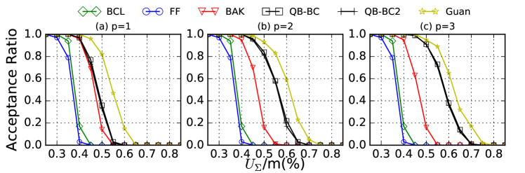
Figure 2: Acceptance ratio comparison on implicit-deadline 8 multiprocessor systems.

6 Conclusion and Extensions

In this paper, we present a general response-time analysis and schedulability-test framework, called $\mathbf{k^{2}Q}$. Thanks to the independence upon the task and platform models in the framework, $\mathbf{k^{2}Q}$ can be viewed as a “block-box” interface that can result in sufficient utilization-based analyses for a wide range of applications in real-time systems under fixed-priority scheduling. We believe that the $\mathbf{k^{2}Q}$ framework has high potential to be adopted to solve several other problems for analyzing other task models in real-time systems with fixed-priority scheduling. The framework can be used, once the corresponding $k$-point last-release scheduling test or response time analysis can be constructed.

Moreover, our proposed frameworks, $\mathbf{k^{2}U}$ and $\mathbf{k^{2}Q}$, provide a solid mathematical foundation for deriving polynomial-time utilization-based schedulability tests and response time analyses almost automatically. That is, utilization-based analyses are almost automatically derived if the schedulability tests can be formulated in the scope of the frameworks. We have demonstrated several applications in this paper. Some models have introduced pretty high dynamics, but we can still handle the response time analysis and schedulability test with proper constructions so that the $\mathbf{k^{2}Q}$ framework is applicable. Therefore, with the presented approach, some difficult schedulability test and response time analysis problems may be solved by building a good (or exact) exponential-time test and using the approximation in the $\mathbf{k^{2}Q}$ framework. With the quadratic and hyperbolic expressions, $\mathbf{k^{2}Q}$ and $\mathbf{k^{2}U}$ frameworks can be used to provide many quantitive features to be measured, like the total utilization bounds, speed-up factors, etc., not only for uniprocessor scheduling but also for multiprocessor scheduling.

When adopting $\mathbf{k^{2}Q}$ for schedulability tests, we assume that $t_{k}$ is specified in Lemma 1. In this paper, we do not explore how to configure the best value of $t_{k}$ and its last release time ordering $\pi$ such that the resulting quadratic form is the best. Therefore, the combination of $\mathbf{k^{2}Q}$/$\mathbf{k^{2}U}$ and the tunable approach by Bini and Buttazzo [12] can be an interesting future research direction, as this can potentially balance the schedulability test and the time complexity for concrete applications. Essentially, this combination is to search the proper settings of different $t_{k}$ values such that the associated last release time ordering $\pi$ can be less pessimistic, as demonstrated by several cases regarding Example 4 in Section 4.

Acknowledgement: This paper has been supported by NSF grant CNS 1527727 and DFG, as part of the Collaborative Research Center SFB876 (http://sfb876.tu-dortmund.de/), and the priority program ”Dependable Embedded Systems” (SPP 1500 - http://spp1500.itec.kit.edu).

Appendix A: Proofs

Proof of Lemma 5. Similar to the proof of Lemma 4, we only have to consider the cases when $U_{i}$ is set to $\frac{x}{k-1}$ to make the schedulability condition the most difficult, where $x=\sum_{i=1}^{k-1}U_{i}$. Suppose that $\frac{C_{k}}{t_{k}}$ is $y$. Then, we are looking for the infimum $x+y$ such that $y>1-(\alpha+\beta)x+0.5\alpha\beta(x^{2}+\frac{x^{2}}{k-1})$.

To solve this, we start with $y=1-(\alpha+\beta)x+0.5\alpha\beta(x^{2}+\frac{x^{2}}{k-1})$. Our objective becomes to minimize $H(x)=x+1-(\alpha+\beta)x+0.5\alpha\beta(x^{2}+\frac{x^{2}}{k-1})$. By finding $\dfrac{dH(x)}{dx}=1-(\alpha+\beta)+\frac{k\alpha\beta x}{k-1}=0$, we know that $x=\frac{(k-1)(\alpha+\beta-1)}{k\alpha\beta}$. Therefore,

$$y= 1-x\left(\alpha+\beta-\frac{0.5k\alpha\beta\frac{(k-1)(\alpha+\beta-1)}{k\alpha\beta}}{k-1}\right)$$

$$= 1-\frac{(k-1)(\alpha+\beta-1)}{k\alpha\beta}(0.5(\alpha+\beta+1))$$

$$= 1-\frac{0.5(k-1)\left((\alpha+\beta)^{2}-1\right)}{k\alpha\beta}.$$ (36)

Since $\alpha+\beta\geq 1$, we know that $x\geq 0$. Whether we should take the above solution only depends on whether $y\geq 0$ or not. If $y\geq 0$, then we can conclude the solution directly; otherwise, if $y<0$, we should set $y$ to $0$. That is, by reorganizing Eq. (36) (under the assumption $\alpha>0$ and $\beta>0$), examining whether $y<0$ is equivalent to testing $(1-\frac{1}{k})\left((\alpha+\beta)^{2}-1\right)>2\alpha\beta$, which implies to test whether $\alpha^{2}+\beta^{2}-1>\frac{1}{k}\left((\alpha+\beta)^{2}-1\right)$. If $\alpha^{2}+\beta^{2}\leq 1$, then $y\geq 0$ since $\alpha^{2}+\beta^{2}-1\leq 0\leq\frac{1}{k}\left((\alpha+\beta)^{2}-1\right)$ due to the assumption $\alpha+\beta\geq 1$. Therefore, there are two cases:
Case 1: If $\alpha^{2}+\beta^{2}>1$ and $k>\frac{(\alpha+\beta)^{2}-1}{\alpha^{2}+\beta^{2}-1}$, then, for such a case $y$ derived from Eq. (36) is negative. We should set $y$ to $0$. The remaining procedure here is the same as in solving the quadratic equation in the proof of Lemma 4 by setting $\frac{C_{k}}{t_{k}}$ to $0$. This leads to the first condition in Eq. (19).
Case 2: If $\alpha^{2}+\beta^{2}\leq 1$ or $k\leq\frac{(\alpha+\beta)^{2}-1}{\alpha^{2}+\beta^{2}-1}$, then, we have the conclusion that $y\geq 0$ and $x\geq 0$. We just have to sum up the above derived $x$ and $y$. This leads to the second condition in Eq. (19) directly.        

Proof of Lemma 6. Definition 3 leads to the following optimization problem:

sup $$C_{k}+\sum_{i=1}^{k-1}\alpha_{i}t_{i}^{*}U_{i}+\sum_{i=1}^{k-1}\beta_{i}C_{i}$$ (37a)

such that $$C_{k}+\sum_{i=1}^{k-1}\alpha_{i}t_{i}^{*}U_{i}+\sum_{i=1}^{j-1}\beta_{i}C_{i}>t_{j}^{*}, \forall j=1,\ldots,k-1,$$ (37b)

$$t_{j}^{*}\geq 0, \forall j=1,\ldots,k-1,$$ (37c)

where $t^{*}_{1},t^{*}_{2},\ldots,t^{*}_{k-1}$ and are variables, $\alpha_{i}$, $\beta_{i}$, $U_{i}$, $C_{i}$ for higher-priority task $\tau_{i}$ and $C_{k}$ are constants. For the rest of the proof, we replace $>$ with $\geq$ in Eq. (37), as the supermum and the maximum are the same when presenting the inequality with $\geq$. We can also further drop the condition $t_{j}^{*}\geq 0$, which just makes the resulting solution more pessimistic. This results in the following linear programming, which has a safe upper bound of Eq. (37),

maximize $$C_{k}+\sum_{i=1}^{k-1}\alpha_{i}t_{i}^{*}U_{i}+\sum_{i=1}^{k-1}\beta_{i}C_{i}$$ (38a)

such that $$C_{k}+\sum_{i=1}^{k-1}\alpha_{i}t_{i}^{*}U_{i}+\sum_{i=1}^{j-1}\beta_{i}C_{i}\geq t_{j}^{*},\forall j=1,\ldots,k-1.$$ (38b)

The linear programming in Eq. (38) (by replacing $>$ with $\geq$ and supremum with maximum) has $k-1$ variables and $k-1$ constraints. Like the proof of Lemma 1, we again adopt the extreme point theorem for linear programming [40] to solve the linear programming. Suppose that $t_{1}^{\dagger},t_{2}^{\dagger},\ldots,t_{k-1}^{\dagger}$ is a feasible solution for the linear programming in (38) and $\hat{t}=\max\{t_{1}^{\dagger},t_{2}^{\dagger},\ldots,t_{k-1}^{\dagger}\}$. By the satisfaction of Eq. (38b), we know that

$$\small C_{k}+\hat{t}\sum_{i=1}^{k-1}\alpha_{i}U_{i}+\sum_{i=1}^{k-1}\beta_{i}C_{i}\geq C_{k}+\sum_{i=1}^{k-1}\alpha_{i}t_{i}^{\dagger}U_{i}+\sum_{i=1}^{k-1}\beta_{i}C_{i}\geq\hat{t}.$$

As a result, we have $\hat{t}\leq\frac{C_{k}+\sum_{i=1}^{k-1}\beta_{i}C_{i}}{1-\sum_{i=1}^{k-1}\alpha_{i}U_{i}}$. That is, any feasible solution of Eq. (38) has $t_{j}^{*}\leq\frac{C_{k}+\sum_{i=1}^{k-1}\beta_{i}C_{i}}{1-\sum_{i=1}^{k-1}\alpha_{i}U_{i}}$ for any $j=1,2,\ldots,k-1$. Under the assumption that $\sum_{i=1}^{k-1}\alpha_{i}U_{i}<1$ and $0\leq\sum_{i=1}^{k-1}\beta_{i}C_{i}$, the above linear programming has a bounded objective function.

The only extreme point solution is to put $C_{k}+\sum_{i=1}^{k-1}\alpha_{i}t_{i}^{*}U_{i}+\sum_{i=1}^{j-1}\beta_{i}C_{i}=t_{j}^{*}$ for every $j=1,2,\ldots,k-1$. Since the objective function is bounded, by the extreme point theorem [40], we know that this extreme point solution is the optimal solution for the linear programming in Eq. (38). For such a solution, we know that

$$\forall j=2,3,\ldots,k-1,\qquad t_{j}^{*}-t_{j-1}^{*}=\beta_{j-1}C_{j-1}.$$ (39)

and

$$t_{1}^{*}=C_{k}+\sum_{i=1}^{k-1}\alpha_{i}U_{i}(t_{1}^{*}+\sum_{\ell=0}^{i-1}\beta_{\ell}C_{\ell}),$$ (40)

where $\beta_{0}$ and $C_{0}$ are defined as $0$ for notational brevity. Therefore, we know that

$$t_{1}^{*}=\frac{C_{k}+\sum_{i=1}^{k-1}\alpha_{i}U_{i}(\sum_{\ell=0}^{i-1}\beta_{\ell}C_{\ell})}{1-\sum_{i=1}^{k-1}\alpha_{i}U_{i}}.$$ (41)

Clearly, the above extreme point solution is always feasible when $\sum_{i=1}^{k-1}\alpha_{i}U_{i}<1$. Therefore, in this extreme point solution, the objective function of the linear programming is

$$t_{1}^{*}+\sum_{i=1}^{k-1}\beta_{i}C_{i}= \frac{C_{k}+\sum_{i=1}^{k-1}\alpha_{i}U_{i}(\sum_{\ell=0}^{i-1}\beta_{\ell}C_{\ell})}{1-\sum_{i=1}^{k-1}\alpha_{i}U_{i}}+\sum_{i=1}^{k-1}\beta_{i}C_{i}$$ (42)

$$= \frac{C_{k}+\sum_{i=1}^{k-1}\beta_{i}C_{i}-\sum_{i=1}^{k-1}\alpha_{i}U_{i}(\sum_{\ell=i}^{k-1}\beta_{\ell}C_{\ell})}{1-\sum_{i=1}^{k-1}\alpha_{i}U_{i}}$$ (43)

which concludes the proof.        

Appendix B: Quadratic Bound for Uniprocessor Constrained-Deadline Tasks

To verify the schedulability of a (constrained-deadline) sporadic real-time task $\tau_{k}$ under fixed-priority scheduling in uniprocessor systems, the time-demand analysis (TDA) developed in [35] can be adopted. That is, if

$$\exists t\mbox{ with }0<t\leq D_{k}{\;\;and\;\;}C_{k}+\sum_{\tau_{i}\in hp(\tau_{k})}\left\lceil{\frac{t}{T_{i}}}\right\rceil C_{i}\leq t,$$ (44)

then task $\tau_{k}$ is schedulable under the fixed-priority scheduling algorithm, where $hp(\tau_{k})$ is the set of tasks with higher priority than $\tau_{k}$, $D_{k}$, $C_{k}$, and $T_{i}$ represent $\tau_{k}$’s relative deadline, worst-case execution time, and period, respectively. For a constrained-deadline task $\tau_{k}$, the schedulability test in Eq. (44) is equivalent to the verification of the existence of $0<t\leq D_{k}$ such that

$$C_{k}+\sum_{\tau_{i}\in hp_{2}(\tau_{k})}C_{i}+\sum_{\tau_{i}\in hp_{1}(\tau_{k})}\left\lceil{\frac{t}{T_{i}}}\right\rceil C_{i}\leq t.$$ (45)

We can then create a virtual sporadic task $\tau_{k}^{\prime}$ with execution time $C_{k}^{\prime}=C_{k}+\sum_{\tau_{i}\in hp_{2}(\tau_{k})}C_{i}$, relative deadline $D_{k}^{\prime}=D_{k}$, and period $T_{k}^{\prime}=D_{k}$. It is clear that the schedulability test to verify the schedulability of task $\tau_{k}^{\prime}$ under the interference of the higher-priority tasks $hp_{1}(\tau_{k})$ is the same as that of task $\tau_{k}$ under the interference of the higher-priority tasks $hp(\tau_{k})$. For notational brevity, suppose that there are $k^{*}-1$ tasks in $hp_{1}(\tau_{k})$.

Theorem 7.

Task $\tau_{k}$ in a sporadic task system with constrained deadlines is schedulable by the fixed-priority scheduling algorithm if $\sum_{i=1}^{k^{*}-1}\frac{C_{i}}{D_{k}}\leq 1$ and

$$\frac{C_{k}^{\prime}}{D_{k}}\leq 1-\sum_{i=1}^{k^{*}-1}U_{i}-\sum_{i=1}^{k^{*}-1}\frac{C_{i}}{D_{k}}+\frac{\sum_{i=1}^{k^{*}-1}U_{i}(\sum_{\ell=i}^{k^{*}-1}C_{\ell})}{D_{k}},$$ (46)

in which the $k^{*}-1$ higher-priority tasks in $hp_{1}(\tau_{k})$ are indexed in a non-decreasing order of $\left(\left\lceil{\frac{D_{k}}{T_{i}}}\right\rceil-1\right)T_{i}$.

Proof. Setting $t_{i}=\left(\left\lceil{\frac{D_{k}}{T_{i}}}\right\rceil-1\right)T_{i}$, and indexing the tasks in a non-decreasing order of $t_{i}$ leads to the satisfaction of Definition 2 with $\alpha_{i}=1$ and $\beta_{i}=1$.        

Corollary 2.

Task $\tau_{k}$ in a sporadic task system with implicit deadlines is schedulable by the RM scheduling algorithm if Lemmas 1, 3, 4, or 5 holds by setting $\frac{C_{k}}{t_{k}}$ as $U_{k}$, $\alpha=1$, and $\beta=1$.

The above result in Corollary 2 leads to the utilization bound $2-\sqrt{2}$ (by using Lemma 5 with $\alpha=1$ and $\beta=1$) for RM scheduling, which is worse than the existing Liu and Layland bound $\ln{2}$ [39].

Appendix C: Multiprocessor DM/RM Scheduling

This part demonstrates how to use the $\mathbf{k^{2}Q}$ framework for multiprocessor global fixed-priority scheduling. We consider that the system has $M$ identical processors. For global fixed-priority scheduling, there is a global queue and a global scheduler to dispatch jobs. We demonstrate the applicability for constrained-deadline and implicit-deadline sporadic systems under global fixed-priority scheduling. Specifically, we will present how to apply the framework to obtain speed-up and capacity augmentation factors for global DM and global RM.

The success of the scheme depends on a corresponding exponential-time test. Here we will use the property to be presented in Lemma 9, based on the forced-forward algorithm proposed by Baruah et al. [7] to characterize the workload of higher-priority tasks. The method in [7] to analyze fixed-priority scheduling is completely different from ours, as they rely on the demand bound functions of the tasks.

The following lemma provides a sufficient test based on the observations by Baruah et al. [7]. The construction of the following lemma is based on a minor change of the forced-forward algorithm.

Lemma 9.

Let $\Delta_{k}^{\max}$ be $\max_{j=1}^{k-1}\{U_{j},\frac{C_{k}}{D_{k}}\}$. Task $\tau_{k}$ in a sporadic task system with constrained deadlines is schedulable by a global fixed-priority (workload conserving) scheduling algorithm on $M$ processors if

$$\forall y\geq 0,\left(\forall 0\leq\omega_{i}\leq T_{i},\forall\tau_{i}\in hp(\tau_{k})\right),\exists t\mbox{ with }0<t\leq D_{k}+y$$

$$\mbox{ such that \;\;}\Delta_{k}^{\max}\cdot(D_{k}+y)+\frac{\sum_{i=1}^{k-1}\omega_{i}\cdot U_{i}+\left\lceil{\frac{t-\omega_{i}}{T_{i}}}\right\rceil C_{i}}{M}\leq t.$$

Proof. This is proved by contrapositive. If task $\tau_{k}$ is not schedulable by the global fixed-priority scheduling, we will show that there exist $y\geq 0$ and $0\leq\omega_{i}\leq T_{i}$ such that for all $0<t\leq D_{k}+y$, the condition $\Delta_{k}^{\max}\cdot(D_{k}+y)+\frac{\sum_{i=1}^{k-1}\omega_{i}\cdot U_{i}+\left\lceil{\frac{t-\omega_{i}}{T_{i}}}\right\rceil C_{i}}{M}>t$ holds. The proof is mainly based on the forced-forward algorithm for the analysis of global DM by Baruah et al. in [7], by making some further annotations.

If $\tau_{k}$ is not schedulable by global DM, let $z_{0}$ be the first time at which task $\tau_{k}$ misses its absolute deadline, i.e., $z_{0}$. Let $z_{1}$ be the arrival time of this job of task $\tau_{k}$. For notational brevity, let this job be $J_{1}$, which arrives at time $z_{1}$ and has not yet been finished at time $z_{0}$. By definition, we know that $z_{0}-z_{1}$ is $D_{k}$. Due to the fixed-priority and workload-conserving scheduling policy and the constrained-deadline setting, removing (1) all the other jobs of task $\tau_{k}$ (except the one arriving at time $z_{1}$), (2) all the jobs arriving no earlier than $z_{0}$, and (3) lower-priority jobs does not change the unschedulability of job $J_{1}$. Therefore, the rest of the proof only considers the jobs from $\tau_{1},\tau_{2},\ldots,\tau_{k}$.

Now, we expand the window of interest by using a slightly different algorithm from that proposed in [7], also illustrated with the notation in Figure 3, as in Algorithm 1. The difference is only in the setting “strictly less than $(z_{\ell-1}-z_{\ell})\cdot\hat{U}_{\ell}$ units”, whereas the setting in [7] uses “strictly less than $(z_{\ell-1}-z_{\ell})\cdot s$ units” for a certain $s$. For notationaly brevity, $\hat{U}_{\ell}$ is the utilization of the task that generates job $J_{\ell}$.

Algorithm 1 (Revised) Forced-Forward Algorithm

1:  for $\ell\leftarrow 2,3,...$ do

2:     let $J_{\ell}$ denote a job that

• arrives at some time-instant $z_{\ell}<z_{\ell-1}$;

• has an absolute deadline after $z_{\ell-1}$;

• has not completed execution by $z_{\ell-1}$; and

• has executed for strictly less than $(z_{\ell-1}-z_{\ell})\cdot\hat{U}_{\ell}$ units over the interval $[z_{\ell},z_{\ell-1})$, where $\hat{U}_{\ell}$ is the utilization of the task that generates job $J_{\ell}$.

3:     if there is no such a job then

4:        $\ell\leftarrow(\ell-1)$; break;

Suppose that the forced-forward algorithm terminates with $\ell$ equals to $\ell^{*}$. We now examine the schedule in the interval $(z_{\ell^{*}},z_{0}]$. Since $J_{1},J_{2},\ldots,J_{\ell^{*}}$ belong to $\tau_{1},\tau_{2},\ldots,\tau_{k}$, we know that $\hat{U}_{\ell}\leq\Delta_{k}^{\max}$ for $\ell=1,2,\ldots,\ell^{*}$. Let $\sigma_{\ell}$ be the total length of the time interval over $(z_{\ell},z_{\ell-1}]$ during which $J_{\ell}$ is executed. By the choice of $J_{\ell}$, it follows that

$$\sigma_{\ell}<(z_{\ell-1}-z_{\ell})\cdot\hat{U}_{\ell}\leq(z_{\ell-1}-z_{\ell})\cdot\Delta_{k}^{\max}.$$

Moreover, all the $M$ processors execute other higher-priority jobs (than $J_{\ell}$) at any other time points in the interval $(z_{\ell},z_{\ell-1}]$ at which $J_{\ell}$ is not executed. Therefore, we know that the maximum amount of time from $z_{\ell^{*}}$ to $z_{0}$, in which not all the $M$ processors execute certain jobs, is at most

$$\small\sum_{\ell=1}^{\ell^{*}}\sigma_{\ell} <\sum_{\ell=1}^{\ell^{*}}(z_{\ell-1}-z_{\ell})\cdot\Delta_{k}^{\max}=(z_{0}-z_{\ell^{*}})\cdot\Delta_{k}^{\max}.$$

Up to here, the treatment is almost identical to that in “Observation 1” in [7]. The following analysis becomes different as we do not intend to use the demand bound function. Now, we replace job $J_{1}$ with another job $J_{1}^{\prime}$ with inflated execution time in the above schedule, where $J_{1}^{\prime}$ is released at time $z_{\ell^{*}}$ with absolute deadline $z_{0}$ and execution time $(z_{0}-z_{\ell^{*}})\cdot\Delta_{k}^{\max}$. According to the above analysis, $J_{1}^{\prime}$ cannot be finished before $z_{0}$ in the above schedule. For each task $\tau_{i}$ for $i=1,2,\ldots,k-1$, in the above schedule, there may be one carry-in job, denoted as $J_{i}^{\flat}$, of $\tau_{i}$ (under the assumption of the schedulability of a higher-priority task $\tau_{i}$) that arrives at time $r_{i}^{\flat}$ with $r_{i}^{\flat}<z_{\ell^{*}}$ and $r_{i}^{\flat}+T_{i}>z_{\ell^{*}}$. Let $d_{i}^{\flat}$ be the next released time of task $\tau_{i}$ after $z_{\ell^{*}}$, i.e., $d_{i}^{\flat}=r_{i}^{\flat}+T_{i}$.

According to the termination condition in the construction of $z_{\ell^{*}}$, if $J_{i}^{\flat}$ exists, we know that at least $(z_{\ell^{*}}-r_{i}^{\flat})\cdot U_{i}$ amount of execution time has been executed before $z_{\ell^{*}}$, and the remaining execution time of job $J_{i}^{\flat}$ to be executed after $z_{\ell^{*}}$ is at most $(d_{i}^{\flat}-z_{\ell^{*}})\cdot U_{i}$. If $J_{i}^{\flat}$ does not exist, then $d_{i}^{\flat}$ is set to $z_{\ell^{*}}$ for notational brevity. Therefore, the amount of workload $W_{i}^{\prime}(t)$ of all the released jobs of task $\tau_{i}$ for $i=1,2,\ldots,k-1$ to be executed in time interval $(z_{\ell}^{*},z_{\ell}^{*}+t)$ is at most

$$W_{i}^{\prime}(t)=(d_{i}^{\flat}-z_{\ell^{*}})\cdot U_{i}+\left\lceil{\frac{t-(d_{i}^{\flat}-z_{\ell^{*}})}{T_{i}}}\right\rceil C_{i}.$$ (47)

The assumption of the unschedulability of job $J_{1}^{\prime}$ (due to the unschedulability of job $J_{1}$) under the global fixed-priority scheduling implies that $J_{1}^{\prime}$ cannot finish its computation at any time between $z_{\ell^{*}}$ and $z_{0}$. This leads to the following (necessary) condition $\Delta_{k}^{\max}(z_{0}-z_{\ell^{*}})+\frac{\sum_{\tau_{i}\in hp(\tau_{k})}W_{i}^{\prime}(t)}{M}>t$ for all $0<t\leq z_{\ell^{*}}-z_{0}$ for the unschedulability of job $J_{1}^{\prime}$.

Therefore, by the existence of $y=z_{1}-z_{\ell^{*}}$ (with $y\geq 0$) and $\omega_{i}=d_{i}^{\flat}-z_{\ell^{*}}$ (with $0\leq\omega_{i}\leq T_{i}$) for $i=1,2,\ldots,k-1$ to enforce the above necessary condition, we reach the conclusion of the proof by contrapositive. That is, task $\tau_{k}$ is schedulable if, for all $y\geq 0$ and any combination of $0\leq\omega_{i}\leq T_{i}$ for $i=1,2,\ldots,k-1$, there exists $0<t\leq D_{k}+y$ with $\Delta_{k}^{\max}(D_{k}+y)+\frac{\sum_{\tau_{i}\in hp(\tau_{k})}\omega_{i}\cdot U_{i}+\left\lceil{\frac{t-\omega_{i}}{T_{i}}}\right\rceil C_{i}}{M}\leq t$.        

The schedulability condition in Lemma 9 may look at the first glance strange. We briefly explain the logical meaning (but informally) here. Suppose we would like to know whether a job of task $\tau_{k}$ arrived at time $r_{k}$ can be finished before/at time $r_{k}+D_{k}$. To better quantify the interference from the higher-priority tasks, we would like to account for the higher-priority jobs arrived prior to $r_{k}$. The variable $y$ defines the extension of the window of interest from $[r_{k},r_{k}+D_{k})$ to $[r_{k}-y,r_{k}+D_{k})$. The variable $\omega_{i}$ defines the maximum residual execution time $\omega_{i}T_{i}$ of a carry-in job of task $\tau_{i}$ that arrives before $r_{k}-y$ and should be executed in the window of interest, i.e., $[r_{k}-y,r_{k}+D_{k})$. If the residual workload is at most $\omega_{i}T_{i}$, the next job can be released at time $r_{k}-y+\omega_{i}$, as shown in the proof. Task $\tau_{k}$ is schedulable by the global fixed-priority scheduling, if, for any combinations of $y\geq 0$ and $0\leq\omega_{i}\leq T_{i},\forall\tau_{i}\in hp(\tau_{k})$, we can always finish the inflated workload $\Delta_{k}^{\max}\cdot(D_{k}+y)$ of task $\tau_{k}$ and the higher-priority workload in the window of interest. For formal explanations, please refer to the formal proof of Lemma 9.

Note that the schedulability condition in Lemma 9 requires to test all possible $y\geq 0$ and all possible settings of $0\leq\omega_{i}\leq T_{i}$ for the higher-priority tasks $\tau_{i}$ with $i=1,2,\ldots,k-1$. Therefore, it needs exponential time (for all the possible combinations of $\omega_{i}$). However, we are not going to directly use the test in Lemma 9 in the paper. We will only use this test to construct the corresponding $k$-point schedulability test under Definition 2.

We present the corresponding polynomial-time schedulability tests for global fixed-priority scheduling. More specifically, we will also analyze the capacity augmentation factors of these tests for global RM and global DM in Corollaries 3 and 4, respectively.

Theorem 8.

Let $U_{k}^{\max}$ be $\max_{j=1}^{k}U_{j}$. Task $\tau_{k}$ in a sporadic task system with implicit deadlines is schedulable by global RM on $M$ processors if

$$U_{k}^{\max}\leq 1-\frac{2}{M}\sum_{i=1}^{k-1}U_{i}+\frac{0.5}{M^{2}}\left((\sum_{i=1}^{k-1}U_{i})^{2}+(\sum_{i=1}^{k-1}U_{i}^{2})\right)$$ (48)

or

$$\frac{\sum_{j=1}^{k-1}U_{j}}{M}\leq\left(\frac{k-1}{k}\right)\left(2-\sqrt{2+2U_{k}^{\max}\frac{k}{k-1}}\right).$$ (49)

Proof. We will show that the schedulability condition in the theorem holds for all possible settings of $y$ and $\omega_{i}$s. Suppose that $y$ and $\omega_{i}$ for $i=1,2,\ldots,k-1$ are given, in which $y\geq 0$ and $0\leq\omega_{i}\leq T_{i}$. Let $t_{k}$ be $T_{k}+y$. Now, we set $t_{i}$ to $\omega_{i}+\left\lfloor{\frac{T_{k}+y-\omega_{i}}{T_{i}}}\right\rfloor T_{i}$ for $i=1,2,\ldots,k-1$ and reindex the tasks such that $t_{1}\leq t_{2}\leq\ldots\leq t_{k}$.

Therefore, if $i<j$, we know that $\omega_{i}\cdot U_{i}+\left\lceil{\frac{t_{j}-\omega_{i}}{T_{i}}}\right\rceil C_{i}\leq\omega_{i}\cdot U_{i}+(\left\lfloor{\frac{t_{i}-\omega_{i}}{T_{i}}}\right\rfloor+1)C_{i}=t_{i}U_{i}+C_{i}$. If $i\geq j$, then $\omega_{i}\cdot U_{i}+\left\lceil{\frac{t_{j}-\omega_{i}}{T_{i}}}\right\rceil C_{i}\leq\omega_{i}\cdot U_{i}+(\left\lceil{\frac{t_{i}-\omega_{i}}{T_{i}}}\right\rceil)C_{i}=t_{i}U_{i}$. The sufficient schedulability condition in Lemma 9 under the given $y$ and $\omega_{i}$s is to verify the existence of $t_{j}\in\left\{{t_{1},t_{2},\ldots t_{k}}\right\}$ such that

$$U_{k}^{\max}(T_{k}+y)+\frac{\sum_{i=1}^{k-1}\omega_{i}\cdot U_{i}+\left\lceil{\frac{t_{j}-\omega_{i}}{T_{i}}}\right\rceil C_{i}}{M}$$ (50)

$$\leq U_{k}^{\max}t_{k}+\frac{\sum_{i=1}^{k-1}U_{i}t_{i}+\sum_{i=1}^{j-1}C_{i}}{M}\leq t_{j}.$$ (51)

By the definition of global RM scheduling (i.e., $T_{k}\geq T_{i}$), we can conclude that $C_{i}=U_{i}T_{i}\leq U_{i}T_{k}\leq U_{i}(T_{k}+y)=U_{i}t_{k}$ for $i=1,2,\ldots,k-1$. Hence, we can safely reformulate the sufficient test by verifying whether there exists $t_{j}\in\left\{{t_{1},t_{2},\ldots t_{k}}\right\}$ such that

$$U_{k}^{\max}t_{k}+\sum_{i=1}^{k-1}\alpha_{i}U_{i}t_{i}+\sum_{i=1}^{j-1}\beta U_{i}t_{k}\leq t_{j},$$ (52)

where $\alpha_{i}=\frac{1}{M}$ and $\beta\leq\frac{1}{M}$ for $i=1,2,\ldots,k-1$. Therefore, we reach the conclusion of the schedulability conditions in Eqs. (48) and (49) by Lemma 3 and Lemma 4 under given $y$ and $\omega_{i}$s, respectively.

The schedulability test in Eq. (52) is independent from the settings of $y$ and $\omega_{i}$s. However, the setting of $y$ and $\omega_{i}$s affects how the $k-1$ higher-priority tasks are indexed. Fortunately, it can be observed that the schedulability tests in Eqs. (48) and (49) are completely independent upon the indexing of the higher-priority tasks. Therefore, no matter how $y$ and $\omega_{i}$s are set, the schedulability conditions in Eqs. (48) and (49) are the corresponding results from the $\mathbf{k^{2}Q}$ framework. As a result, we can reach the conclusion.        

Corollary 3.

The capacity augmentation factor of global RM for a sporadic system with implicit deadlines is $\frac{3+\sqrt{7}}{2}\approx 2.823$.

Proof. Suppose that $\sum_{\tau_{i}}\frac{C_{i}}{MT_{i}}\leq\frac{1}{b}$ and $U_{k}^{\max}\leq\max_{\tau_{i}}U_{i}\leq\frac{1}{b}$. The right-hand side of Eq. (49) converges to $2-\sqrt{2+U_{k}^{\max}}$ when $k\rightarrow\infty$ Therefore, by Eq. (49), we can guarantee the schedulability of task $\tau_{k}$ if $\frac{1}{b}\leq 2-\sqrt{2+\frac{2}{b}}$. This is equivalent to solving $x=2-\sqrt{2+2x}$, which holds when $x=3-\sqrt{7}$. Therefore, we reach the conclusion of the capacity augmentation factor $\frac{3+\sqrt{7}}{2}\approx 2.823$.        

Theorem 9.

Let $\Delta_{k}^{\max}$ be $\max_{j=1}^{k-1}\{U_{j},\frac{C_{k}}{D_{k}}\}$. Task $\tau_{k}$ in a sporadic task system with constrained deadlines is schedulable by a global fixed-priority scheduling on $M$ processors if $\sum_{i=1}^{k}U_{i}\leq M$, $\sum_{i=1}^{k-1}\frac{C_{i}}{D_{k}}\leq M$, and

$$\Delta_{k}^{\max}\leq 1-\frac{1}{M}\sum_{i=1}^{k-1}\left(U_{i}+\frac{C_{i}}{D_{k}}\right)+\frac{1}{M^{2}}\left(\sum_{i=1}^{k-1}U_{i}(\sum_{\ell=i}^{k-1}\frac{C_{\ell}}{D_{k}})\right),$$ (53)

where the $k-1$ higher-priority tasks are ordered in a non-increasing order of their periods.

Proof. This is due to a similar proof to that of Theorem 8 and Lemma 9, by applying Lemma 1 with $t_{k}=D_{k}+y$, $\alpha_{i}=\frac{1}{M}$, and $\beta_{i}=\frac{1}{M}$, under the worst-case last release time ordering, $\frac{\beta_{i}C_{i}}{\alpha_{i}U_{i}}=T_{i}$ non-increasingly, in Lemma 2. Therefore, for a given $y\geq 0$, if $\Delta_{k}^{\max}\leq 1-\frac{1}{M}\sum_{i=1}^{k-1}\left(U_{i}+\frac{C_{i}}{D_{k}+y}\right)+\frac{1}{M^{2}}\left(\sum_{i=1}^{k-1}U_{i}(\sum_{\ell=i}^{k-1}\frac{C_{\ell}}{D_{k}+y})\right)$, task $\tau_{k}$ is schedulable by the global fixed-scheduling. By the assumption $\sum_{i=1}^{k-1}U_{i}\leq M$, we know that $C_{i}\frac{\sum_{\ell=1}^{i}U_{\ell}}{M}\leq C_{i}$. Therefore,

$$-\frac{1}{M}\sum_{i=1}^{k-1}\frac{C_{i}}{D_{k}+y}+\frac{1}{M^{2}}\left(\sum_{i=1}^{k-1}U_{i}(\sum_{\ell=i}^{k-1}\frac{C_{\ell}}{D_{k}+y})\right)$$

$$= \frac{1}{D_{k}+y}\frac{1}{M}\left(-\sum_{i=1}^{k-1}C_{i}+\sum_{i=1}^{k-1}C_{i}\left(\frac{\sum_{\ell=1}^{i}U_{\ell}}{M}\right)\right)$$

is minimized when $y$ is $0$. As a result, the above schedulability condition is the worst when $y$ is $0$.        

Corollary 4.

The capacity augmentation factor and the speed-up factor of global DM by using Theorem 9 for a sporadic system with constrained deadlines is 3.

Proof. If $\sum_{i=1}^{k}U_{i}\leq M$ or $\sum_{i=1}^{k-1}\frac{C_{i}}{D_{k}}\leq M$ is violated, the capacity augmentation factor is already $1$. Therefore, we focus on the case that task $\tau_{k}$ does not pass the schedulability condition in Eq. (53). That is,

$$\Delta_{k}^{\max}> 1-\frac{1}{M}\sum_{i=1}^{k-1}\left(U_{i}+\frac{C_{i}}{D_{k}}\right)+\frac{1}{M^{2}}\left(\sum_{i=1}^{k-1}U_{i}(\sum_{\ell=i}^{k-1}\frac{C_{\ell}}{D_{k}})\right)$$

$$\geq 1-\frac{1}{M}\sum_{i=1}^{k-1}\left(U_{i}+\frac{C_{i}}{D_{k}}\right).$$

This means that the unschedulability of task $\tau_{k}$ under global DM implies that either $\Delta_{k}^{\max}>\frac{1}{3}$, $\frac{1}{M}\sum_{i=1}^{k-1}U_{i}>\frac{1}{3}$, or $\frac{1}{M}\sum_{i=1}^{k-1}\frac{C_{i}}{D_{k}}>\frac{1}{3}$, by the pigeonhole principle. Therefore, we conclude the factor $3$.        

Remarks: The utilization bound in Eq. (49) is analytically better than the best known utilization-based schedulability test $\sum_{j=1}^{k}U_{j}\leq\frac{M}{2}(1-U_{k}^{\max})+U_{k}^{\max}$ for global RM by Bertogna et al. [10], since $\frac{(1-x)}{2}\leq 2-\sqrt{2+2x}$ when $0\leq x\leq 1$.

The capacity augmentation factor $2.823$ in Corollary 3 is weaker than the result $2.668$ by Lundberg [41]. However, we would like to point out the incompleteness in the proof in [41]. In the proof of the extreme task set, the argument in Page 150 in [41] concludes that task $\tau_{n}$ is more difficult to be schedulable due to the increased interference of task $\tau_{n-1}$ to task $\tau_{n}$ after the transformation. The argument was not correctly proved and can be optimistic since the increased interference has to be analyzed in all time points in the analysis window, whereas the analysis in [41] only considers the interference in a specific interval length. Without analyzing the resulting interference in all time points in the analysis window, task $\tau_{n}$ after transformation may still have chance to finish earlier due to the potential reduction of the interference at earlier time points.

The speed-up factor $3$ provided in Corollary 4 is asymptotically the same as the result by Baruah et al. [7]. The speed-up factor $3$ in [7] requires a pseudo polynomial-time test, whereas we show that a simple test in Eq. (53) can already yield the speed-up factor $3$ in $O(k\log k)$ time complexity.

We limit our attention here for the global RM/DM scheduling. Andersson et al. [2] propose the RM-US[$\varsigma$] algorithm, which gives the highest priority to tasks $\tau_{i}$s with $U_{i}>\varsigma$, and otherwise assigns priorities by using RM. Our analysis here can also be applied for the RM-US[$\varsigma$] algorithm with some modifications in the proofs by setting $\varsigma=\frac{2}{3+\sqrt{7}}\approx 0.3542$.

Figure 3: Notation of the forced-forward algorithm for the analysis of global fixed-priority scheduling.

Appendix D: Response-Time for Periodic Tasks with Jitters

A periodic task (with jitters) $\tau_{i}$ is defined by its period $T_{i}$, its execution time $C_{i}$, its relative deadline $D_{i}$ and, its jitter $L_{i}$. The jitter problem arises when we consider some flexibility to delay the job arrival for a certain bounded length $L_{i}$. Such a problem has also been studied in the literature, such as [9, 3].

We focus on uniprocessor fixed-priority scheduling here. The busy window concept has also been used for the schedulability analysis of fixed-priority scheduling [3]. For the $h$-th job of task $\tau_{k}$ in the busy window, the finishing time $R_{k,h}$ is the minimum $t$ such that

$$hC_{k}+\sum_{i=1}^{k-1}\left\lceil{\frac{t+L_{i}}{T_{i}}}\right\rceil C_{i}\leq t.$$

The $h$-th job of task $\tau_{k}$ arrives at time $\max\{(h-1)T_{k}-L_{k},0\}$, and, hence, its response time is $R_{k,h}-\max\{(h-1)T_{k}-L_{k},0\}$. The busy window of task $\tau_{k}$ finishes on the $h$-th job if $R_{k,h}\leq\max\{hT_{k}-L_{k},0\}$.

Lemma 10.

$R_{k,h}$ is upper bounded by finding the maximum

$$t_{k}=hC_{k}+\sum_{i=1}^{k-1}L_{i}U_{i}+\sum_{i=1}^{k-1}t_{i}U_{i}+\sum_{i=1}^{k-1}C_{i},$$ (54)

among all possible least release time orderings of the $k-1$ higher-priority tasks with $0\leq t_{1}\leq t_{2}\leq\cdots\leq t_{k-1}\leq t_{k}$ and

$$hC_{k}+\sum_{i=1}^{k-1}L_{i}U_{i}+\sum_{i=1}^{k-1}t_{i}U_{i}+\sum_{i=1}^{j-1}C_{i}>t_{j}, \forall j=1,2,\ldots,k-1.$$ (55)

Proof. Suppose that $R_{k,h}$ is known. Then, the last release of task $\tau_{i}$ in the busy window before $R_{k,h}$ is at time $t_{i}=(\left\lceil{\frac{R_{k,h}+L_{i}}{T_{i}}}\right\rceil-1)T_{i}-L_{i}$. We can index the $k-1$ higher-priority tasks by $t_{i}$ non-decreasingly. By the definition of $t_{i}$, we know that $(\left\lceil{\frac{R_{k,h}+L_{i}}{T_{i}}}\right\rceil-1)C_{i}=\frac{t_{i}+L_{i}}{T_{i}}T_{i}U_{i}=t_{i}U_{i}+L_{i}U_{i}$. That is, the accumulative workload of task $\tau_{i}$ from $0$ to $t_{i}$ is exactly $L_{i}U_{i}+t_{i}U_{i}$. Due to the indexing rule, and the known $R_{k,h}$ we can now conclude the conditions in Eqs. (54) and (55).

However, it should be noted that the last release time ordering is actually unknown since $R_{k,h}$ is unknown. Therefore, we have to consider all possible last release time orderings.        

Lemma 11.

Suppose that $\sum_{i=1}^{k-1}U_{i}\leq 1$. Then, for any $h\geq 1$ and $C_{k}>0$, we have

$$R_{k,h}\leq\frac{hC_{k}+\sum_{i=1}^{k-1}(C_{i}+L_{i}U_{i})-\sum_{i=1}^{k-1}U_{i}(\sum_{\ell=i}^{k-1}C_{\ell})}{1-\sum_{i=1}^{k-1}U_{i}},$$ (56)

where the $k-1$ higher-priority tasks are ordered in a non-increasing order of their periods.

Proof. This comes from the above discussions with $\alpha_{i}=1$, $\beta_{i}=1$ in Lemma 10 by applying Lemmas 6 and 7 when $\sum_{i=1}^{k-1}U_{i}<1$. The case when $\sum_{i=1}^{k-1}U_{i}=1$ has a safe upper bound $R_{k,h}=\infty$ in Eq. (56).        

Theorem 10.

Suppose that $\sum_{i=1}^{k}U_{i}\leq 1$. The worst-case response time of task $\tau_{k}$ is at most

$$R_{k}\leq \frac{\sum_{i=1}^{k-1}(C_{i}+L_{i}U_{i})-\sum_{i=1}^{k-1}U_{i}(\sum_{\ell=i}^{k-1}C_{\ell})}{1-\sum_{i=1}^{k-1}U_{i}},$$ (57)

$$+\max\left\{\frac{h^{*}C_{k}}{1-\sum_{i=1}^{k-1}U_{i}},\frac{(h^{*}+1)C_{k}}{1-\sum_{i=1}^{k-1}U_{i}}-h^{*}T_{k}+L_{k}\right\}$$

where the $k-1$ higher-priority tasks are ordered in a non-increasing order of their periods and $h^{*}=\left\lfloor{\frac{L_{k}}{T_{k}}}\right\rfloor+1$.

Proof. By the definition of $h^{*}$, we know that $(h^{*}-1)T_{k}-L_{k}\leq 0$, whereas $h^{*}T_{k}-L_{k}>0$. When $h\leq h^{*}$, we know that $\max\left\{(h^{*}-1)T_{k}-L_{k},0\right\}$ is $0$. Therefore, $R_{k,h}-0$ is maximized when $h$ is set to $h^{*}$ for any $h\leq h^{*}$.

The first-order derivative of $R_{k,h}-((h-1)T_{k}-L_{k})$ with respect to $h$ when $h\geq h^{*}+1$ is $\frac{C_{k}}{1-\sum_{i=1}^{k-1}U_{i}}-T_{k}=\frac{C_{k}-(1-\sum_{i=1}^{k-1}U_{i})T_{k}}{1-\sum_{i=1}^{k-1}U_{i}}$. Similar to the proof of Theorem 4, we know that setting $R_{k,h}-(h-1)T_{k}$ is maximized when $h$ is set to $h^{*}+1$ for any $h\geq h^{*}+1$.

As a result, we only have to evaluate the two cases by setting $h$ as $h^{*}$ or $h^{*}+1$. One of them is the worst-case response time. The formulation in Eq. (57) simply compares these two response times.        

Appendix E: Schedulability for Generalized Multi-Frame

A generalized multi-frame real-time task $\tau_{i}$ with $m_{i}$ frames is defined as a task with an array $(C_{i,0},D_{i,0},T_{i,0},C_{i,1},D_{i,1},T_{i,1},\ldots,C_{i,m_{i}-1},D_{i,m_{i}-1},T_{i,m_{i}-1})$ of different execution times, different relative deadlines, and the minimal inter-arrival time of the next frame [46, 8]. The execution time of the $j$-th job of task $\tau_{i}$ is defined as $C_{i,(j\mod m_{i})}$. If a job of the $j$-th frame of task $\tau_{i}$ is released at time $t$, the earliest time that task $\tau_{i}$ can release the next $(j+1)\mod m_{i}$ frame is at time $t+T_{j}$. Here, we consider only constrained-deadline cases, in which $D_{i,j}\leq T_{i,j}$.

Takada and Sakamura [46] provide an exact test with exponential-time complexity for such a problem under task-level fixed-priority scheduling, in which each task is assigned with one static priority level. For this section, we will focus on such a setting. Specifically, we are interested in analyzing the schedulability of the $h$-th frame of task $\tau_{k}$ under the given task priority ordering. It was shown that the critical instant theorem of periodic task systems by Liu and Layland [39] does not work anymore for generalized multi-frame systems. Fortunately, as shown in Theorem 2 in [46], the critical instant of the $h$-th frame of task $\tau_{k}$ is to release a certain frame of a higher priority task $\tau_{i}$ at the same time, and the subsequent frames of task $\tau_{i}$ as early as possible. In fact, this problem has been recently proved to be co-NP hard in the strong sense in [45].

For completeness, the test with exponential time complexity by Takada and Sakamura [46] will be presented in Lemma 12 by using our notation. We define ${\sc rbf}(i,q,t)$ as the maximum workload of task $\tau_{i}$ released within an interval length $t$ starting from the $q$-th frame. That is,

$${\sc rbf}(i,q,t)=\sum_{j=q}^{\theta(i,q,t)}C_{i,(j\mod m_{i})},$$ (58)

where $\theta(i,q,t)$ is the smallest $\ell$ such that $\sum_{j=q}^{\ell}T_{i,(j\mod m_{i})}\geq t$. That is, $\theta(i,q,t)$ is the last frame released by task $\tau_{i}$ before $t$ under the critical instant starting with the $q$-th frame of task $\tau_{i}$.

Lemma 12.

The $h$-th frame of task $\tau_{k}$ in a generalized multiframe task system with constrained deadlines is schedulable by a fixed-priority scheduling on a uniprocessor system if

$$\forall q_{i}\in\left\{{0,1,\ldots,m_{i}-1}\right\},\forall i=1,2,\ldots,k-1$$

$$\exists 0<t\leq D_{k,h},\;\;\;\;C_{k,h}+\sum_{i=1}^{k-1}{\sc rbf}(i,q_{i},t)\leq t.$$

Proof. This is a reformulation of the test by Takada and Sakamura [46].        

Since the test in Lemma 12 requires exponential-time complexity, an approximation by using Maximum Interference Function (MIF) was proposed in [46] to provide a sufficient test efficiently. Instead of testing all possible combinations of $q_{i}$, a simple strategy is to use $rbf(i,t)=\max_{q=0}^{m_{i}-1}rbf(i,q,t)$ to approximate the test in Lemma 12. This results in a pseudo-polynomial-time test. Guan et al. [28] have recently provided proofs to show that such an approximation is with a speed-up factor of $2$.

We will use a different way to build our analysis by constructing the $k$-point last-release schedulability test in Definition 2. The idea is very simple. If task $\tau_{i}$ starts with its $q$-th frame, we can find and define

$$t_{i,q}=\sum_{j=q}^{\theta(i,q,D_{k,h})-1}T_{i,(j\mod m_{i})}$$

as the last release time of task $\tau_{i}$ before $D_{k,h}$. Therefore, for the given $D_{k,h}$, we are only interested in these $m_{i}$ last release times of task $\tau_{i}$. We need a safe function for estimating their workload. More precisely, we want to find two constants $U_{i,k,h}$ and $C_{i,k,h}$ such that $U_{i,k,h}\cdot t_{i,q}\geq rbf(i,q,t_{i,q})$ and $U_{i,k,h}\cdot t_{i,q}+C_{i,k,h}\geq rbf(i,q,t_{i,q}+\epsilon)=rbf(i,q,D_{k,h})$. This means that no matter which frame of task $\tau_{i}$ is the first frame in the critical instant, we can always bound the workload from task $\tau_{i}$ by using $U_{i,k,h}\cdot t+C_{i,k,h}$ for the points that we are interested to test. According to the above discussions, we can set

$$U_{i,k,h}=\max_{q=0,1,\ldots,m_{i}-1}\max\left\{\frac{rbf(i,q,t_{i,q})}{t_{i,q}}\right\}$$ (59)

$$C_{i,k,h}=\max_{q=0,1,\ldots,m_{i}-1}{\sc rbf}(i,q,D_{k,h})-U_{i,k,h}\cdot t_{i,q}$$ (60)

Now, we can reorganize the schedulability test to link to Definition 2.

Lemma 13.

The $h$-th frame of task $\tau_{k}$ in a generalized multiframe task system with constrained deadlines is schedulable by a fixed-priority scheduling on a uniprocessor system if the following condition holds: For any last release ordering $\pi$ of the $k-1$ higher-priority tasks with $t_{1,q_{1}}\leq t_{2,q_{2}}\leq\cdots\leq t_{k-1,q_{k-1}}\leq t_{k}=D_{k,h}$, there exists $t_{j,q_{j}}$ such that

$$C_{k,h}+\sum_{i=1}^{k-1}U_{i,k,h}\cdot t_{i,q_{i}}+\sum_{i=1}^{j-1}C_{i,k,h}\leq t_{j,q_{j}},$$ (61)

where $U_{i,k,h}$ and $C_{i,k,h}$ are defined in Eqs. (59) and (60), respectively.

Proof. This comes from the above discussions and Lemma 12.        

The choice of $q_{i}$ only affects the last release ordering of the $k-1$ higher-priority tasks, but it does not change the constants $U_{i,k,h}$ and $C_{i,k,h}$. Therefore, Lemma 13 satisfies Definition 2 by removing the indexes $q$, but the worst-case last release time ordering has to be considered.

Theorem 11.

Suppose that $\sum_{i=1}^{k-1}C_{i,k,h}<D_{k,h}$. The $h$-th frame of task $\tau_{k}$ in a generalized multiframe task system with constrained deadlines is schedulable by a scheduling algorithm on a uniprocessor system if the following condition holds

$$\frac{C_{k,h}}{D_{k,h}}\leq 1-\sum_{i=1}^{k-1}U_{i,k,h}-\frac{\sum_{i=1}^{k-1}(C_{i,k,h}-U_{i,k,h}(\sum_{\ell=i}^{k-1}C_{\ell,k,h}))}{D_{k,h}},$$ (62)

in which the $k-1$ higher-priority tasks are indexed in a non-increasing order of $\frac{C_{i,k,h}}{U_{i,k,h}}$ of task $\tau_{i}$.

Proof. The schedulability test (under a specified last release time ordering $\pi$) in Lemma 13 satisfies Definition 2 with $\alpha_{i}=\beta_{i}=1$. Therefore, we can apply Lemmas 1 and 2 to reach the conclusion of the proof.        

A naïve implementation to calculate $t_{i,q}$ and $rbf(i,q,t)$ requires $O(m_{i})$ time complexity. Therefore, calculating $U_{i,k,h}$ and $C_{i,k,h}$ requires $O(m_{i}^{2})$ time complexity with such an implementation. It can be calculated with better data structures and implementations to achieve $O(m_{i})$ time complexity. That is, we first calculate $t_{i,0}$ and $rbf(i,0,t_{i,0})$ in $O(m_{i})$ time complexity. The overall time complexity to calculate the following $t_{i,q}$ and $rbf(i,q,t_{i,q})$ can be done in $O(m_{i})$ by using simple algebra. Therefore, the time complexity of the schedulability test in Theorem 11 is $O(\sum_{i=1}^{k-1}m_{i}+k\log k)$.

Remarks: Although we focus ourselves on generalized multi-frame task systems in this section, it can be easily seen that our approach can also be adopted to find polynomial-time tests based on the request bound function presented in [28]. Since such functions have been shown useful for schedulability tests in more generalized task models, including the digraph task model [44], the recurring real-time task model [6], etc., the above approach can also be applied for such models by quantifying the utilization (e.g., $U_{i,k,h}$) and the execution time (e.g., $C_{i,k,h}$) of task $\tau_{i}$ based on the limited options of the last release times before the deadline (e.g., $D_{k,h}$ in generalized multi-frame) to be tested.

Appendix F: Acyclic and Multi-Mode Tasks

This section considers the acyclic model, proposed in [1]. That is, each task $\tau_{i}$ is specified only by its utilization $U_{i}$. An instance of task $\tau_{i}$ can have different worst-case execution times and different relative deadlines. If an instance of task $\tau_{i}$ arrives at time $t$ with execution time $C_{i,t}$, its relative deadline is $\frac{C_{i,t}}{U_{i}}$, and the next instance of task $\tau_{i}$ can only be released after $t+\frac{C_{i,t}}{U_{i}}$.

For systems with known modes, we can also define a multi-mode task system. A multi-mode task $\tau_{i}$ with $m_{i}$ modes is denoted by a set of triplet: $\tau_{i}=\{\tau_{i,0}=\left\{{C_{i,0},D_{i,0},T_{i,0}}\right\},\tau_{i,1}=\left\{{C_{i,1},D_{i,1},T_{i,1}}\right\},\ldots,\tau_{i,m_{i}-1}=\left\{{C_{i,m_{i}-1},D_{i,m_{i}-1},T_{i,m_{i}-1}}\right\}\}$ to specify the worst-case execution time $C_{i,j}$, the minimum inter-arrival time $T_{i,j}$, and the relative deadline $D_{i,j}$ of the corresponding task mode $\tau_{i,j}$. For a multi-mode task $\tau_{i}$, when a job of mode $\tau_{i,j}$ is released at time $t$, this job has to be finished no later than its absolute deadline at time $t+D_{i,j}$, and the next release time of task $\tau_{i}$ is no earlier than $t+T_{i,j}$. We only consider systems with constrained deadlines, in which $D_{i,j}\leq T_{i,j}$. This model is studied in our paper [31]. The difference between this model and the generalized multi-frame model is that the system can switch arbitrarily among any two modes if the temporal seperation constraints in the multi-mode model are respected.

We will focus on mode-level fixed-priority scheduling on uniprocessor scheduling in this section. Suppose that we are testing whether task $\tau_{k,h}$ can be feasibly scheduled. Let $hp(\tau_{k,h})$ be the set of task mode $\tau_{k,h}$ and the other task modes with higher priority than task mode $\tau_{k,h}$. It is important to note that $\tau_{k,h}$ is also in $hp(\tau_{k,h})$ for the simplicity of presentation. For notational brevity, we assume that there are $k-1$ tasks with higher-priority task modes than $\tau_{k,h}$. Moreover, for the rest of this section, we implicitly assume that the tasks in $hp(\tau_{k,h})\setminus\left\{{\tau_{k,h}}\right\}$ are schedulable by the mode-level fixed-priority scheduling algorithm under testing.

Let $load(i,t)$ be the maximum workload of task $\tau_{i}$ (by considering all the task modes $\tau_{i,j}\in hp(\tau_{k,h})$) released from $0$ to $t$ such that the next mode can be released at time $t$. That is, let $n_{i,q}$ be a non-negative integer to denote the number of times that task mode $\tau_{i,q}$ is released, in which

$$load(i,t)=\max_{\tau_{i,q}\in hp(\tau_{k,h})}\{ \sum_{q}n_{i,q}C_{i,q}$$

$$\qquad\mbox{ s.t. }\sum_{q}n_{i,q}T_{i,q}\leq t\}.$$

We denote $C_{i}^{\max}(\tau_{k,h})$ the maximum mode execution time among the higher-priority modes of task $\tau_{i}$ than task mode $\tau_{k,h}$, i.e., $\max_{\tau_{i,j}\in hp(\tau_{k,h})}C_{i,j}$ for a given index $i$. Similarly, we denote $U_{i}^{\max}(\tau_{k,h})$ the maximum mode utilization among the higher-priority modes of task $\tau_{i}$ than task mode $\tau_{k,h}$, i.e., $\max_{\tau_{i,j}\in hp(\tau_{k,h})}\frac{C_{i,j}}{T_{i,j}}$ for a given index $i$. For notational brevity, since we define $C_{i}^{\max}(\tau_{k,h})$ and $U_{i}^{\max}(\tau_{k,h})$ by referring to $\tau_{k,h}$, we will simplify the notation by using $C_{i}^{\max}$ and $U_{i}^{\max}$, respectively, for the rest of this section.

Suppose that the last release of task $\tau_{i}$ in the window of interest is at $t_{i}$. We define the request bound function for such a case as follows:

$$rbf(i,t_{i},t)=\begin{cases}load(i,t_{i})&\mbox{ if }t\leq t_{i}\\ load(i,t_{i})+C_{i}^{\max}&\mbox{ otherwise}.\end{cases}$$ (63)

Lemma 14.

Task $\tau_{k,h}$ in a multi-mode task system with constrained deadlines is schedulable by a mode-level fixed-priority scheduling algorithm on uniprocessor systems if

$$\forall y\geq 0,{\;\;\forall 0\leq t_{i}<y+D_{k,h}\forall i=1,2,\ldots,k-1\;\;}$$

$$\exists t,\;0<t\leq y+D_{k,h},\qquad C_{k,h}+load(k,y)+\sum_{i=1}^{k-1}rbf(i,t_{i},t)\leq t.$$

Proof. This is proved by contrapositive. Suppose that $\tau_{k,h}$ misses its deadline firstly at time $d_{k,h}$. We know that this job of $\tau_{k,h}$ arrives to the system at time $a_{1}=d_{k,h}-D_{k,h}$. Due to the scheduling policy, we know that the processor is busy executing jobs in $hp(\tau_{k,h})$ (recall that $\tau_{k,h}$ is also in $hp(\tau_{k,h})$) from $a_{1}$ to $d_{k,h}$. Let $a_{0}$ be the last time point in the above schedule before $a_{1}$ such that the processor is idle or executing any job with lower priority than $\tau_{k,h}$. It is clear that $a_{0}$ is well-defined. Therefore, the processor executes only jobs in $hp(\tau_{k,h})$ from $a_{0}$ to $d_{k,h}$. We denote $a_{1}-a_{0}$ as $y$. Let the last release of the task modes of task $\tau_{i}$ before $d_{k,h}$ be $a_{0}+t_{i}$. If task $\tau_{i}$ does not have any release, we set $t_{i}$ to $0$. Therefore, we have $0\leq t_{i}<y+D_{k,h}$.

Without loss of generality, we set $a_{0}$ to $0$. Therefore, the workload requested by the modes of task $\tau_{i}$ at any time $t$ before (and at) $t_{i}$ is no more than $load(i,t)$. Moreover, the workload released by the modes of task $\tau_{i}$ at any time $t$ after $t_{i}$ is no more than $load(i,t_{i})+C_{i}^{\max}$. As a result, the function $rbf(i,t_{i},t)$ defined in Eq. (63) is a safe upper bound of the workload requested by task $\tau_{i}$ upt to time $t$.

By the definition of the task model, task mode $\tau_{k,h}$ and the other higher-priority task modes of task $\tau_{k}$ may also release some workload before $a_{1}$, in which the workload is upper bounded by $load(k,y)$. The assumption of non-schedulability of task $\tau_{k,h}$ in the above schedule and the busy execution in the interval $(a_{0},d_{k,h}]$ implies that the above workload at any point $t$ in the interval $(a_{0},d_{k,h}]$ is larger than $t$. Therefore, we know that

$$\exists y\geq 0,{\;\;\exists 0\leq t_{i}<y+D_{k,h}\forall i=1,2,\ldots,k-1\;\;}$$

$$\forall t,\;0<t\leq y+D_{k,h},\;\;C_{k,h}+load(k,y)+\sum_{i=1}^{k-1}rbf(i,t_{i},t)>t,$$

which concludes the proof by contrapositive.        

Evaluating $load(i,t)$ is in fact equivalent to the unbounded knapsack problem (UKP). The UKP problem is to select some items in a collection of items with specified weights and profits so that the total weight of the selected items is less than or equal to a given limit (called knapsack) and total profit of the selected items is maximized, in which an item can be selected unbounded multiple times. The definition of $load(i,t)$ is essentially an unbounded knapsack problem, by considering $t$ as the knapsack constraint, the minimum inter-arrival time (period) of a task mode as the weight of an item, and the execution time of a task mode as the profit of the item.

Lemma 15.

$$load(i,t)\leq U_{i}^{\max}\cdot t.$$ (64)

Proof. It has been shown in [42] that an upper bound of the above unbounded knapsack problem is $\left(\max_{\tau_{i,j}\in hp(\tau_{k,h})}\{\frac{C_{i,j}}{T_{i,j}}\}\right)\cdot t=U_{i}^{\max}\cdot t$, which completes the proof.        

By Lemma 14 and Lemma 15, we can now apply the $\mathbf{k^{2}Q}$ framework to obtain the polynomial-time schedulability test in the following theorems.

Theorem 12.

For a given task $\tau_{i}$ and a task mode $\tau_{k,h}$ under testing, let $C_{i}^{\max}=\max_{\tau_{i,j}\in hp(\tau_{k,h})}C_{i,j}$ and $U_{i}^{\max}=\max_{\tau_{i,j}\in hp(\tau_{k,h})}\frac{C_{i,j}}{T_{i,j}}$. Suppose that there are $k-1$ tasks with higher-priority modes than task mode $\tau_{k,h}$. Let $\Delta_{k}^{\max}$ be $\max\{\max_{\tau_{k,j}\in hp(\tau_{k,h})}\{\frac{C_{k,j}}{T_{k,j}}\},\frac{C_{k,h}}{D_{k,h}}\}$. Suppose that $\sum_{i=1}^{k-1}C_{i}^{\max}<D_{k,h}$. Task $\tau_{k,h}$ in a multi-mode task system with constrained deadlines is schedulable by a mode-level fixed-priority scheduling algorithm on a uniprocessor system if $\sum_{i=1}^{k-1}U_{i}^{\max}\leq 1$ and

$$\Delta_{k}^{\max}\leq 1-\sum_{i=1}^{k-1}U_{i}^{\max}-\frac{\sum_{i=1}^{k-1}(C_{i}^{\max}-U_{i}^{\max}(\sum_{\ell=i}^{k-1}C_{\ell}^{\max}))}{D_{k,h}},$$ (65)

in which the $k-1$ higher-priority tasks are indexed in a non-increasing order of $\frac{C_{i}^{\max}}{U_{i}^{\max}}$ of task $\tau_{i}$.

Proof. Suppose that $t_{i}$ is given for each task $\tau_{i}$. For the given $t_{i}$, we can define the last release time ordering, in which $t_{1}\leq t_{2}\leq\ldots\leq t_{k-1}\leq D_{k,h}+y=t_{k}$. By Lemma 15, we can pessimistically rephrase the schedulability test in Lemma 14 to verify whether there exists $t_{j}\in\left\{{t_{1},t_{2},\ldots,t_{k}}\right\}$ such that $\Delta_{k}^{\max}(D_{k,h}+y)+\sum_{i=1}^{k-1}U_{i}^{\max}t_{i}+\sum_{i=1}^{j-1}C_{i}^{\max}\leq t_{j}$. Therefore, we reach Definition 2 with $\alpha_{i}=1$ and $\beta_{i}=1$, and, hence, can apply Lemmas 1 and 2. . Moreover, with the same argument in the proof of Theorem 9, we know that the resulting schedulability condition is the worst if $y$ is $0$ under the assumption $\sum_{i=1}^{k-1}U_{i}^{\max}\leq 1$.        

Theorem 13.

For a given task $\tau_{i}$ and a task mode $\tau_{k,h}$ under testing, let $U_{i}^{\max}=\max_{\tau_{i,j}\in hp(\tau_{k,h})}\frac{C_{i,j}}{T_{i,j}}$. Suppose that there are $k-1$ tasks with higher-priority modes than task mode $\tau_{k,h}$. Let $U_{k}^{\max}$ be $\max\{\max_{\tau_{k,j}\in hp(\tau_{k,h})}\{\frac{C_{k,j}}{T_{k,j}}\},\frac{C_{k,h}}{T_{k,h}}\}$. Suppose that $\sum_{i=1}^{k}U_{i}^{\max}\leq 1$. Task $\tau_{k,h}$ in a multi-mode task system with implicit deadlines is schedulable by the mode-level RM scheduling algorithm on a uniprocessor system if the following condition holds

$$U_{k}^{\max}\leq 1-2\sum_{i=1}^{k-1}U_{i}^{\max}+0.5\left((\sum_{i=1}^{k-1}U_{i}^{\max})^{2}+(\sum_{i=1}^{k-1}(U_{i}^{\max})^{2})\right),$$ (66)

or

$$\sum_{i=1}^{k-1}U_{i}^{\max}\leq\left(\frac{k-1}{k}\right)\left(2-\sqrt{2+2U_{k}^{\max}\frac{k}{k-1}}\right),$$ (67)

or

$$U_{k}^{\max}+\sum_{i=1}^{k-1}U_{i}^{\max}\leq\begin{cases}\left(\frac{k-1}{k}\right)\left(2-\sqrt{4-\frac{2k}{k-1}}\right),&\mbox{ if }k>3\\ 1-\frac{(k-1)}{2k}&\mbox{otherwise}.\end{cases}$$ (68)

Proof. Due to the RM property, we know that $T_{i,j}\leq T_{k,h}$ if $\tau_{i,j}$ is in $hp(\tau_{k,h})$. Therefore, $C_{i}^{\max}\leq T_{k,h}U_{i}^{\max}$. We now reach the conditions in Lemmas 3,  4, and 5 with $\alpha=1$ and $\beta=1$. The three conditions are directly from these lemmas.        

Note that the above tests assume implicitly that the tasks in $hp(\tau_{k,h})$ are already tested to be schedulable under the scheduling policy. Therefore, we have to apply the results in Theorems 12 and 13 by testing all the task modes from the highest priority to the lowest priority. The following theorem provides the utilization bound for testing the whole task set in linear time for mode-level RM scheduling.

Corollary 5.

Suppose that $\sum_{i=1}^{k}U_{i}\leq 1$. A system with $k$ acyclic tasks with utilization $U_{1},U_{2},\ldots,U_{k}$ is schedulable by the mode-level RM scheduling algorithm on a uniprocessor system if

$$\sum_{i=1}^{k}U_{i}\leq\begin{cases}\left(\frac{k-1}{k}\right)\left(2-\sqrt{4-\frac{2k}{k-1}}\right),&\mbox{ if }k>3\\ 1-\frac{(k-1)}{2k}&\mbox{otherwise}.\end{cases}$$ (69)

or

$$0\leq 1-U_{k}-2\sum_{i=1}^{k-1}U_{i}+0.5\left((\sum_{i=1}^{k-1}U_{i})^{2}+(\sum_{i=1}^{k-1}U_{i}^{2})\right),$$ (70)

where task $\tau_{k}$ is the task with the minimum utilization among the $k$ tasks.

Proof. This comes with similar arguments in Theorem 13. Adopting the utilization bound in Eq. (69) does not need to consider the ordering of the tasks. However, the quadratic bound in Eq. (70) changes for different settings of $U_{k}$. Let $\sum_{i=1}^{k}U_{i}$ be a given constant $H_{1}$ and $\sum_{i=1}^{k}U_{i}^{2}$ be $H_{2}$. Then, the quadratic bound in Eq. (70) becomes $1-2H_{1}+U_{k}+0.5H_{1}^{2}+0.5H_{2}-0.5U_{k}^{2}$. The first order derivative of the quadratic bound with respect to $U_{k}$ is $1-U_{k}$, which implies that the minimum $U_{k}$ leads to the worst condition in the quadratic bound in Eq. (70) under the condition $U_{k}\leq 1$.        

The result in Eq. (69) in Corollary 5 is the same as the utilization bound $2-\sqrt{2}$ (when $k\rightarrow\infty$) in [1, 31] for such a task model. Our results here are more generic than [1] and can also be easily applied for any (mode-level or task-level) fixed-priority scheduling.

References

• [1] T.Β F. Abdelzaher, V.Β Sharma, and C.Β Lu. A utilization bound for aperiodic tasks and priority driven scheduling. IEEE Trans. Computers, 53(3):334–350, 2004.
• [2] B.Β Andersson, S.Β K. Baruah, and J.Β Jonsson. Static-priority scheduling on multiprocessors. In Real-Time Systems Symposium (RTSS), pages 193–202, 2001.
• [3] N.Β Audsley, A.Β Burns, M.Β Richardson, K.Β Tindell, and A.Β Wellings. Applying new scheduling theory to static priority pre-emptive scheduling. Software Engineering Journal, 8(5):284–292, Sep 1993.
• [4] T.Β P. Baker. Multiprocessor EDF and deadline monotonic schedulability analysis. In IEEE Real-Time Systems Symposium, pages 120–129, 2003.
• [5] T.Β P. Baker. An analysis of fixed-priority schedulability on a multiprocessor. Real-Time Systems, 32(1-2):49–71, 2006.
• [6] S.Β K. Baruah. The non-cyclic recurring real-time task model. In Proceedings of the 31st IEEE Real-Time Systems Symposium, RTSS 2010, San Diego, California, USA, November 30 - December 3, 2010, pages 173–182, 2010.
• [7] S.Β K. Baruah, V.Β Bonifaci, A.Β Marchetti-Spaccamela, and S.Β Stiller. Improved multiprocessor global schedulability analysis. Real-Time Systems, 46(1):3–24, 2010.
• [8] S.Β K. Baruah, D.Β Chen, S.Β Gorinsky, and A.Β K. Mok. Generalized multiframe tasks. Real-Time Systems, 17(1):5–22, 1999.
• [9] S.Β K. Baruah, D.Β Chen, and A.Β K. Mok. Jitter concerns in periodic task systems. In Proceedings of the 18th IEEE Real-Time Systems Symposium (RTSS ’97), December 3-5, 1997, San Francisco, CA, USA, pages 68–77, 1997.
• [10] M.Β Bertogna, M.Β Cirinei, and G.Β Lipari. New schedulability tests for real-time task sets scheduled by deadline monotonic on multiprocessors. In Principles of Distributed Systems, 9th International Conference, OPODIS, pages 306–321, 2005.
• [11] M.Β Bertogna, M.Β Cirinei, and G.Β Lipari. New schedulability tests for real-time task sets scheduled by deadline monotonic on multiprocessors. In Principles of Distributed Systems, pages 306–321. Springer, 2006.
• [12] E.Β Bini and G.Β C. Buttazzo. Schedulability analysis of periodic fixed priority systems. IEEE Trans. Computers, 53(11):1462–1473, 2004.
• [13] E.Β Bini, G.Β C. Buttazzo, and G.Β M. Buttazzo. Rate monotonic analysis: the hyperbolic bound. Computers, IEEE Transactions on, 52(7):933–942, 2003.
• [14] E.Β Bini, T.Β H.Β C. Nguyen, P.Β Richard, and S.Β K. Baruah. A response-time bound in fixed-priority scheduling with arbitrary deadlines. IEEE Transactions on Computers, 58(2):279, 2009.
• [15] E.Β Bini, A.Β Parri, and G.Β Dossena. A quadratic-time response time upper bound with a tightness property. In IEEE Real-Time Systems Symposium (RTSS), 2015.
• [16] A.Β Burchard, J.Β Liebeherr, Y.Β Oh, and S.Β H. Son. New strategies for assigning real-time tasks to multiprocessor systems. pages 1429–1442, 1995.
• [17] S.Β Chakraborty, S.Β KΓΌnzli, and L.Β Thiele. Approximate schedulability analysis. In IEEE Real-Time Systems Symposium, pages 159–168, 2002.
• [18] J.-J. Chen, W.-H. Huang, and C.Β Liu. Evaluate and compare two utilization-based schedulability-test frameworks for real-time systems. Computing Research Repository (CoRR), 2015. http://arxiv.org/abs/1505.02155.
• [19] J.-J. Chen, W.-H. Huang, and C.Β Liu. $k^{2}U$: A general framework from k-point effective schedulability analysis to utilization-based tests. In IEEE Real-Time Systems Symposium, RTSS, 2015.
• [20] J.-J. Chen, W.-H. Huang, and C.Β Liu. k2U: A general framework from k-point effective schedulability analysis to utilization-based tests. In Real-Time Systems Symposium (RTSS), 2015.
• [21] J.-J. Chen, W.-H. Huang, and C.Β Liu. Automatic parameter derivations in $k^{2}U$ framework. Computing Research Repository (CoRR), 2016. http://arxiv.org/abs/1605.00119.
• [22] R.Β Davis, T.Β Rothvoß, S.Β Baruah, and A.Β Burns. Quantifying the sub-optimality of uniprocessor fixed priority pre-emptive scheduling for sporadic tasksets with arbitrary deadlines. In Real-Time and Network Systems (RTNS), pages 23–31, 2009.
• [23] R.Β I. Davis and A.Β Burns. Improved priority assignment for global fixed priority pre-emptive scheduling in multiprocessor real-time systems. Real-Time Systems, 47(1):1–40, 2011.
• [24] R.Β I. Davis, T.Β Feld, V.Β Pollex, and F.Β Slomka. Schedulability tests for tasks with variable rate-dependent behaviour under fixed priority scheduling. In 20th IEEE Real-Time and Embedded Technology and Applications Symposium, pages 51–62, 2014.
• [25] R.Β I. Davis, A.Β Zabos, and A.Β Burns. Efficient exact schedulability tests for fixed priority real-time systems. Computers, IEEE Transactions on, 57(9):1261–1276, 2008.
• [26] S.Β K. Dhall and C.Β L. Liu. On a real-time scheduling problem. Operations Research, 26(1):127–140, 1978.
• [27] N.Β Fisher and S.Β K. Baruah. A fully polynomial-time approximation scheme for feasibility analysis in static-priority systems with arbitrary relative deadlines. In ECRTS, pages 117–126, 2005.
• [28] N.Β Guan, C.Β Gu, M.Β Stigge, Q.Β Deng, and W.Β Yi. Approximate response time analysis of real-time task graphs. In Proceedings of the IEEE 35th IEEE Real-Time Systems Symposium, pages 304–313, 2014.
• [29] N.Β Guan, M.Β Stigge, W.Β Yi, and G.Β Yu. New response time bounds for fixed priority multiprocessor scheduling. In IEEE Real-Time Systems Symposium, pages 387–397, 2009.
• [30] C.-C. Han and H.Β ying Tyan. A better polynomial-time schedulability test for real-time fixed-priority scheduling algorithms. In Real-Time Systems Symposium (RTSS), pages 36–45, 1997.
• [31] W.-H. Huang and J.-J. Chen. Techniques for schedulability analysis in mode change systems under fixed-priority scheduling. In Real-Time Computing Systems and Applications (RTCSA, 2015.
• [32] T.-W. Kuo, L.-P. Chang, Y.-H. Liu, and K.-J. Lin. Efficient online schedulability tests for real-time systems. Software Engineering, IEEE Transactions on, 29(8):734–751, 2003.
• [33] C.-G. Lee, L.Β Sha, and A.Β Peddi. Enhanced utilization bounds for qos management. IEEE Trans. Computers, 53(2):187–200, 2004.
• [34] J.Β P. Lehoczky. Fixed priority scheduling of periodic task sets with arbitrary deadlines. In RTSS, pages 201–209, 1990.
• [35] J.Β P. Lehoczky, L.Β Sha, and Y.Β Ding. The rate monotonic scheduling algorithm: Exact characterization and average case behavior. In IEEE Real-Time Systems Symposium, pages 166–171, 1989.
• [36] J.Β Li, J.Β Chen, K.Β Agrawal, C.Β Lu, C.Β Gill, and A.Β Saifullah. Analysis of federated and global scheduling for parallel real-time tasks. In Euromicro Conference on Real-Time Systems, 2014.
• [37] C.Β Liu and J.Β Anderson. Task scheduling with self-suspensions in soft real-time multiprocessor systems. In Proceedings of the 30th Real-Time Systems Symposium, pages 425–436, 2009.
• [38] C.Β Liu and J.-J. Chen. Bursty-interference analysis techniques for analyzing complex real-time task models. In IEEE Real-Time Systems Symposium, 2014.
• [39] C.Β L. Liu and J.Β W. Layland. Scheduling algorithms for multiprogramming in a hard-real-time environment. Journal of the ACM (JACM), 20(1):46–61, 1973.
• [40] D.Β G. Luenberger and Y.Β Ye. Linear and nonlinear programming, volume 116. Springer, 2008.
• [41] L.Β Lundberg. Analyzing fixed-priority global multiprocessor scheduling. In Real-Time and Embedded Technology and Applications Symposium (RTAS), pages 145–153, 2002.
• [42] S.Β Martello and P.Β Toth. Knapsack problems: algorithms and computer implementations. John Wiley & Sons, Inc., 1990.
• [43] C.Β Phillips, C.Β Stein, E.Β Torng, and J.Β Wein. Optimal time-critical scheduling via resource augmentation. In Proc. of the 29th ACM Symposium on Theory of Computing, pages 140–149, 1997.
• [44] M.Β Stigge, P.Β Ekberg, N.Β Guan, and W.Β Yi. The digraph real-time task model. In 17th IEEE Real-Time and Embedded Technology and Applications Symposium, RTAS 2011, Chicago, Illinois, USA, 11-14 April 2011, pages 71–80, 2011.
• [45] M.Β Stigge and W.Β Yi. Hardness results for static priority real-time scheduling. In 24th Euromicro Conference on Real-Time Systems ECRTS, pages 189–198, 2012.
• [46] H.Β Takada and K.Β Sakamura. Schedulability of generalized multiframe task sets under static priority assignment. In 4th International Workshop on Real-Time Computing Systems and Applications (RTCSA, pages 80–86, 1997.
• [47] J.Β Wu, J.Β Liu, and W.Β Zhao. On schedulability bounds of static priority schedulers. In Real-Time and Embedded Technology and Applications Symposium (RTAS), pages 529–540, 2005.