Pomeranchuk instability and Bose condensation of scalar quanta in a Fermi liquid

Abstract

We study excitations in a normal Fermi liquid with a local scalar interaction. Spectrum of bosonic scalar-mode excitations is investigated for various values and momentum dependence of the scalar Landau parameter $f_{0}$ in the particle-hole channel. For $f_{0}>0$ the conditions are found when the phase velocity on the spectrum of the zero sound acquires a minimum at a non-zero momentum. For $-1<f_{0}<0$ there are only damped excitations, and for $f_{0}<-1$ the spectrum becomes unstable against a growth of scalar-mode excitations (a Pomeranchuk instability). An effective Lagrangian for the scalar excitation modes is derived after performing a bosonization procedure. We demonstrate that the Pomeranchuk instability may be tamed by the formation of a static Bose condensate of the scalar modes. The condensation may occur in a homogeneous or inhomogeneous state relying on the momentum dependence of the scalar Landau parameter. Then we consider a possibility of the condensation of the zero-sound-like excitations in a state with a non-zero momentum in Fermi liquids moving with overcritical velocities, provided an appropriate momentum dependence of the Landau parameter $f_{0}(k)>0$.

I Introduction

The theory of normal Fermi liquids was built up by Landau FL , see in textbooks LP1981 ; Nozieres ; GP-FL . The Fermi liquid approach to the description of nuclear systems was developed by Migdal Mjump ; M67 . In the Fermi liquid theory the low-lying excitations are described by several phenomenological Landau parameters. Pomeranchuk has shown in Ref. Pomeranchuk that Fermi liquids are stable only if some inequalities on the values of the Landau parameters are fulfilled.

In this work we study low-lying scalar excitation modes (density-density fluctuations) in the cold normal Fermi liquids for various values and momentum behavior of the scalar Landau parameter $f_{0}$ in the particle-hole channel. We assume that an interaction in the particle-particle channel is repulsive and the system is, therefore, stable against pairing in an s-wave state. An induced p-wave pairing to be possible at very low temperatures $T<T_{{\rm c},p}$, see Refs. pwave-pairing , can be precluded by the assumption that the temperature of the system is small but above $T_{{\rm c},p}$.

For $f_{0}>0$ the conditions will be found when the phase velocity of the spectrum possesses a minimum at a non-zero momentum. This means that the spectrum satisfies the Landau necessary condition for superfluidity. As a consequence this may lead to a condensation of zero-sound-like excitations with a non-zero momentum in moving Fermi liquids with the velocity above the Landau critical velocity Vexp95 . Similar phenomena may occur in moving He-II, cold atomic gases, and other moving media, like rotating neutron stars, cf. Refs. Pitaev84 ; V93 ; Melnikovsky ; BP12 ; KV2015 ; Kolomeitsev:2015dua . For $-1<f_{0}<0$ excitations are damped, for $f_{0}<-1$ the spectrum is unstable against the growth of zero-sound-like modes and hydrodynamic modes. Up to now it was thought that for $f_{0}<-1$ the mechanical stability condition is violated that results in exponential buildup of the density fluctuations. In hydrodynamic terms the condition $f_{0}<-1$ implies that the speed of the first sound becomes imaginary. This would lead to an exponential growth of the aerosol-like mixture of droplets and bubbles (spinodal instability). In a one-component Fermi liquid spinodal instability results in a mixed liquid-gas like stationary state determined by the Maxwell construction if the pressure has a van der Waals form as a function of the volume. In the isospin symmetric nuclear matter (if the Coulomb interaction is neglected) the liquid-gas phase transition might occur RMS ; SVB for the baryon densities $0.3n_{0}\stackrel{{\scriptstyle\scriptstyle<}}{{\phantom{}{}_{\sim}}}n\stackrel{{\scriptstyle\scriptstyle<}}{{\phantom{}{}_{\sim}}}0.7n_{0}$, where $n_{0}$ is the nuclear saturation density. In a many-component system a mechanical instability is accompanied by a chemical instability, see Ref. Margueron:2002wk . The inclusion of the Coulomb interaction, see Refs. Ravenhall:1983uh ; Maruyama:2005vb , leads to a possibility of the pasta phase in the neutron star crusts for densities $0.3n_{0}\stackrel{{\scriptstyle\scriptstyle<}}{{\phantom{}{}_{\sim}}}n\stackrel{{\scriptstyle\scriptstyle<}}{{\phantom{}{}_{\sim}}}0.7n_{0}$.

The key point of this work is that we suggest an alternative description of unstable zero-sound-like modes which might be realized at certain conditions. We demonstrate that for $f_{0}<-1$ instability may result in an accumulation of a static Bose condensate of the scalar field. The condensate amplitude is stabilized by the repulsive self-interaction. The condensation may occur in the homogeneous either in inhomogeneous state depending on the momentum dependence of the Landau parameter $f_{0}(k)$. In the presence of the condensate the Fermi liquid proves to be stable.

The work is organized as follows. In Sect. II we study spectrum of excitations in a one-component Fermi liquid in the scalar channel in dependence on $f_{0}(k)$. In Sect. III we bosonize the local interaction and suggest an effective Lagrangian for the self-interacting scalar modes. In Sect. IV we study Pomeranchuk instability for $f_{0}<-1$ and suggest a novel possibility of the occurrence of the static Bose-condensate which leads to a stabilization of the system. In Sect. V we consider condensation of scalar excitations in moving Fermi liquids with repulsive interactions. Concluding remarks are formulated in Sect. VI.

II Excitations in a Fermi liquid

II.1 Landau particle-hole amplitude.

Consider the simplest case of a one-component Fermi liquid of non-relativistic fermions. As discussed in the Introduction, we assume that the system is stable against pairing. The particle-hole scattering amplitude on the Fermi surface obeys the equation LP1981 ; Nozieres ; GP-FL ; M67

$$\widehat{T}_{\rm ph}(\vec{n}\,^{\prime},\vec{n};q)=\widehat{\Gamma}^{\omega}(\vec{n}\,^{\prime},\vec{n})$$

$$\quad+\langle\widehat{\Gamma}^{\omega}(\vec{n}\,^{\prime},\vec{n}^{\prime\prime})\,\mathcal{L}_{\rm ph}(\vec{n}\,^{\prime\prime};q)\,\widehat{T}_{\rm ph}(\vec{n}\,^{\prime\prime},\vec{n};q)\rangle_{\vec{n}\,^{\prime\prime}}\,,$$ (1)

where $\vec{n}$ and $\vec{n}\,^{\prime}$ are directions of fermion momenta before and after scattering and $q=(\omega,\vec{k})$ is the momentum transferred in the particle-hole channel. The brackets stand for averaging over the momentum direction $\vec{n}$

$$\langle\dots\rangle_{\vec{n}}=\intop\frac{{\rm d}\Omega_{\vec{n}}}{4\,\pi}\big{(}\dots\big{)}\,,$$ (2)

and the particle-hole propagator is

$$\mathcal{L}_{\rm ph}(\vec{n};q)=\intop_{-\infty}^{+\infty}\!\!\frac{{\rm d}\epsilon}{2\pi i}\!\!\intop_{0}^{+\infty}\!\!\frac{{\rm d}p\,p^{2}}{\pi^{2}}\,{G}(p_{{\rm F}+})\,{G}(p_{{\rm F}-})\,,$$ (3)

where we denoted $p_{{\rm F}\pm}=(\epsilon\pm\omega/2,p_{\rm F}\,\vec{n}\pm\vec{k}/2)$ and $p_{\rm F}$ stands for the Fermi momentum. The quasiparticle contribution to the full Green’s function is given by

$$G(\epsilon,\vec{p})=\frac{a}{\epsilon-\xi_{\vec{p}}+i\,0\,{\rm sign}\epsilon}\,,\quad\xi_{\vec{p}}=\frac{p^{2}-p_{\rm F}^{2}}{2\,m_{\rm F}^{*}}\,.$$ (4)

Here $m^{*}_{\rm F}$ is the effective fermion mass, and the parameter $a$ determines a quasiparticle weight in the fermion spectral density, $0<a\leq 1$, which is expressed through the retarded fermion self-energy $\Sigma_{\rm F}^{R}(\epsilon,p)$ as $a^{-1}=1-(\partial\Re\Sigma_{\rm F}^{R}/\partial\epsilon)_{0}$. The full Green’s function contains also a regular background part $G_{\rm reg}$, which is encoded in the renormalized particle-hole interaction $\hat{\Gamma}^{\omega}$ in Eq. (1).

The interaction in the particle-hole channel can be written as

$$\hat{\Gamma}^{\omega}(\vec{n}\,^{\prime},\vec{n})=\Gamma^{\omega}_{0}(\vec{n}\,^{\prime}\vec{n})\,\sigma^{\prime}_{0}\sigma_{0}+\Gamma^{\omega}_{1}(\vec{n}\,^{\prime}\vec{n})\,(\vec{\sigma}\,^{\prime}\vec{\sigma})\,.$$ (5)

The matrices $\sigma_{j}$ with $j=0,\dots,3$ act on incoming fermions while the matrices $\sigma^{\prime}_{j}$ act on outgoing fermions; $\sigma_{0}$ is the unity matrix and other Pauli matrices $\sigma_{1,2,3}$ are normalized as ${\rm Tr}\sigma_{i}\sigma_{j}=2\delta_{ij}$. We neglect here the spin-orbit interaction, which is suppressed for small transferred momenta $q\ll p_{\rm F}$. The scalar and spin amplitudes in Eq. (5) can be expressed in terms of dimensionless scalar and spin Landau parameters

$$\tilde{f}(\vec{n}\,^{\prime},\vec{n}) =a^{2}\,N_{0}\Gamma_{0}^{\omega}(\vec{n}\,^{\prime},\vec{n})\,,$$

$$\tilde{g}(\vec{n}\,^{\prime},\vec{n}) =a^{2}\,N_{0}\Gamma_{1}^{\omega}(\vec{n}\,^{\prime},\vec{n})\,,$$ (6)

where the normalization constant is chosen as in applications to atomic nuclei M67 ; SaperFayans ; MSTV90 with the density of states at the Fermi surface, $N_{0}=N(n=n_{0})$, taken at the nuclear saturation density $n_{0}$ and $N(n)=\frac{m_{\rm F}^{*}(n)\,p_{\rm F}(n)}{\pi^{2}}$. Such a normalization is at variance with that used, e.g., in Refs. FL ; LP1981 ; Nozieres ; GP-FL . Their parameters are related to ours defined in Eq. (6) as $f=N\,\tilde{f}/N_{0}$ and $g=N\,\tilde{g}/N_{0}$.

The Landau parameters can be expanded in terms of the Legendre polynomials $P_{l}(\vec{n}\cdot\vec{n}\,^{\prime})$,

$$\tilde{f}(\vec{n}\,^{\prime},\vec{n})=\sum_{l}\tilde{f}_{l}\,P_{l}(\vec{n}\cdot\vec{n}\,^{\prime})\,,$$ (7)

and the similar expression exists for the parameter $\tilde{g}$. The Landau parameters $\tilde{f}_{0,1}$, $\tilde{g}_{0,1}$ can be directly related to observables GP-FL . For instance, the effective quasiparticle mass is given by LP1981 ; Nozieres

$$\frac{m^{*}_{\rm F}}{m_{\rm F}}=1+a^{2}\,N\,\overline{\Gamma_{0}(\cos\theta)\cos\theta}=1+\frac{1}{3}f_{1}\,,$$ (8)

where the bar denotes the averaging over the azimuthal and polar angles. The positiveness of the effective mass is assured by fulfillment of the Pomeranchuk condition $f_{1}>-3$. Note that the traditional normalization of the Landau parameters (6) depends explicitly on the effective mass $m^{*}$ through the density of states $N$. Therefore, it is instructive to rewrite Eq. (8) using the definition in Eq. (6)

$$\frac{m^{*}_{\rm F}}{m_{\rm F}}=\frac{1}{1-\frac{1}{3}\frac{m_{\rm F}}{m^{*}_{{\rm F}}(n_{0})}\tilde{f}_{1}}\,.$$ (9)

From this relation we obtain the constraint $\tilde{f}_{1}<3\,m^{*}_{{\rm F}}(n_{0})/m_{\rm F}$ for the effective mass to remain positive and finite; otherwise the effective mass tends to infinity in the point where $\tilde{f}_{1}=3\,m^{*}_{{\rm F}}(n_{0})/m_{\rm F}$. Thus, for the systems where one expects a strong increase of the effective mass, the normalization (6) of the Landau parameters would be preferable. A large increase of the effective fermion mass may be a sign of a quantum phase transition dubbed in Refs. KhodelShaginian ; Khodel:2011dx as a fermion condensation. The latter is connected with the appearance of multi-connected Fermi surfaces. As demonstrated in Ref. Voskresensky:2000px if such a phenomenon occurs in neutron star interiors, e.g., at densities close to the critical density of a pion condensation, this would trigger efficient direct Urca cooling processes. On the other hand, right from the dispersion relation follows that

$$\frac{m^{*}_{\rm F}}{m_{\rm F}}=\frac{1-(\partial\Re\Sigma_{\rm F}^{R}/\partial\epsilon)_{\rm F}}{1+(\partial\Re\Sigma_{\rm F}^{R}/\partial\epsilon_{p}^{0})_{\rm F}}\,,$$ (10)

where $\epsilon_{p}^{0}=p^{2}/2m_{\rm F}$. Thereby, the Landau parameter $\tilde{f}_{1}$ can be expressed via the energy-momentum derivatives of the fermion self-energy.

Below we focus our study on effects associated with the zero harmonic $\tilde{f}_{0}$ in the expansion of $\Gamma^{\omega}_{0}$ as a function of $(\vec{n}\vec{n}\,^{\prime})$. Then the solution of Eq. (1) is

$$\widehat{T}_{\rm ph}(\vec{n}\,^{\prime},\vec{n};q) = T_{{\rm ph},0}(q)\,\sigma^{\prime}_{0}\,\sigma_{0}+T_{{\rm ph},1}(q)\,(\vec{\sigma}\,^{\prime}\vec{\sigma})\,,$$

$$T_{{\rm ph},0(1)}(q) = \frac{1}{1/\Gamma^{\omega}_{0(1)}-\langle\mathcal{L}_{\rm ph}(\vec{n};q)\rangle_{\vec{n}}}\,.$$ (11)

The averaged particle-hole propagator is expressed through the Lindhard’s function

$$\langle\mathcal{L}_{\rm ph}(\vec{n};q)\rangle_{\vec{n}}=-a^{2}N\Phi\big{(}\frac{\omega}{v_{\rm F}\,k},\frac{k}{p_{\rm F}}\big{)}\,,$$ (12)

where

$$\Phi(s,x) =\frac{z_{-}^{2}-1}{4(z_{+}-z_{-})}\ln\frac{z_{-}+1}{z_{-}-1}$$

$$-\frac{z_{+}^{2}-1}{4(z_{+}-z_{-})}\ln\frac{z_{+}+1}{z_{+}-1}+\frac{1}{2}\,.$$ (13)

Here and below we use the dimensionless variables $z_{\pm}=s\pm x/2$, $s=\omega/kv_{\rm F}$, $x=k/p_{\rm F}$. For real $s$ the Lindhard’s function acquires an imaginary part

$$\Im\Phi(s,x)=\left\{\begin{array}[]{ccl}\frac{\pi}{2}\,s&,&0\leq s\leq 1-\frac{x}{2}\\ \frac{\pi}{4x}(1-z_{-}^{2})&,&1-\frac{x}{2}\leq s\leq 1+\frac{x}{2}\\ 0&,&\mbox{otherwise}\end{array}\right.\,.$$ (17)

For $s\gg 1$,

$$\Phi(s,x)\approx-1/(3\,z_{+}\,z_{-})\,.$$ (18)

For $x\ll 1$ the function $\Phi$ can be expanded as

$$\Phi(s,x)\approx 1+\frac{s}{2}\log\frac{s-1}{s+1}-\frac{x^{2}}{12\left(s^{2}-1\right)^{2}}\,,$$ (19)

and if we expand it further for $s\ll 1$ we get

$$\Phi(s,x)\approx 1+i\frac{\pi}{2}s-s^{2}-\frac{x^{2}}{12}-\frac{s^{4}}{3}-\frac{x^{2}s^{2}}{6}-\frac{x^{4}}{240}\,.$$ (20)

At finite temperatures the function $\Phi$ should be replaced by the temperature dependent Lindhard function $\Phi_{T}$ calculated in Ref. Voskresensky:1982vd . Generalization of expansion (20) for low temperature case ($T\ll\epsilon_{\rm F}$) is given by

$$\Phi_{T}(s,x,t)=\Phi(s,x)\,\Big{(}1-\frac{\pi^{2}}{12}t^{2}\Big{)}\,,$$ (21)

where $t=T/\epsilon_{\rm F}$ and $\epsilon_{\rm F}=p_{\rm F}^{2}/2m_{\rm F}^{*}$ is the Fermi energy. For high temperatures $(T\gg\epsilon_{\rm F}$) we have

$$\Phi_{T}(0,x,t)=\frac{2}{3\,t}\Big{(}1-\frac{x^{2}}{6\,t}-\frac{1}{3\,\sqrt{2\pi\,t^{3}}}\Big{)}\,.$$ (22)

The amplitudes (11) possess simple poles and logarithmic cuts. For the amplitude $T_{{\rm ph},0}$ the pole is determined by the equation

$$\frac{1}{f_{0}}=-\Phi\big{(}\frac{\omega}{v_{\rm F}\,k},\frac{k}{p_{\rm F}}\big{)}\,.$$ (23)

Similar equation exists in $g$-channel (with replacement $f_{0}\to g_{0}$. Analytical properties of the solution (23) have been studied in Sadovnikova .

Expanding the retarded particle-hole amplitude $T^{R}_{{\rm ph},0}(q)$ near the spectrum branch

$$T^{R}_{{\rm ph},0}(q) \approx\frac{2\omega(k)V^{2}(k)}{(\omega+i0)^{2}-\omega^{2}(k)}\,,$$

$$V^{-2}(k) =a^{2}N\frac{\partial\Phi}{\partial\omega^{2}}\Big{|}_{\omega(k)}\,,$$ (24)

we identify the quantity $D^{R}(\omega,k)=[(\omega+i0)^{2}-\omega^{2}(k)]^{-1}$ as the retarded propagator of a boson with the dispersion relation $\omega=\omega(k)$ and the quantity $V(k)$ as the effective vertex of the fermion-boson interaction.

For the neutron matter the parameters $f=f_{nn}$, $g=g_{nn}$ are the neutron-neutron Landau scalar and spin parameters. Generalization to the two component system, e.g., to the nuclear matter of arbitrary isotopic composition is formally simple M67 . Then the amplitude should be provided with four indices ($nn$, $pp$, $np$ and $pn$). However, equations for the partial amplitudes do not decouple. For the isospin-symmetric nuclear system with the omitted Coulomb interaction the situation is simplified since then $f_{nn}=f_{pp}$ and $f_{np}=f_{pn}$. In this case one usually presents $\Gamma_{0}^{\omega}$ in Eqs. (5) and (6) as $\Gamma_{0}^{\omega}=(\tilde{f}+\tilde{f}^{\prime}\vec{\tau}^{\prime}\vec{\tau})/a^{2}N_{0}$, and $\Gamma_{1}^{\omega}=(\tilde{g}+\tilde{g}^{\prime}\vec{\tau}^{\prime}\vec{\tau})/a^{2}N_{0}$, where $\tau_{i}$ are isospin Pauli matrices. Quantities $f$ and $f^{\prime}$ (and similarly $g$ and $g^{\prime}$) are expressed through $f_{nn}$ and $f_{np}$ as $f=\frac{1}{2}(f_{nn}+f_{np})$ and $f^{\prime}=\frac{1}{2}(f_{nn}-f_{np})$. The amplitudes of these four channels ($f$, $f^{\prime}$, $g$, $g^{\prime}$) decouple, cf. Ref. AAB . The excitation modes are determined by four equations similar to Eq. (23), now with $2f_{0}$, $2f_{0}^{\prime}$, $2g_{0}$ and $2g_{0}^{\prime}$. Presence of the small Coulomb potential modifies the low-lying modes determined by Eq. (23) (now with $f_{0}$, $f_{0}^{\prime}$, $g_{0}$ and $g_{0}^{\prime}$) only at low momenta AAB . We will ignore the Coulomb effects in our exploratory study.

We discuss now the properties of the bosonic modes for different values of the Landau parameter $f_{0}$.

II.2 Repulsive interaction ($f_{0}>0$). Zero sound.

For $f_{0}>0$ there exists a real solution of Eq. (23) such that for $k\to 0$ the ratio $\omega_{s}(k)/k$ tends to a constant. Such a solution is called a zero sound. The zero sound exists as a quasi-particle mode in the high frequency limit $\omega\gg 1/\tau_{\rm col}$, where $\tau_{\rm col}\propto\epsilon_{\rm F}/T^{2}$ is the fermion collision time. In the opposite limit it turns into a hydrodynamic (first) sound Pethick-Ravenhall88 . At some value $k_{\rm lim}\stackrel{{\scriptstyle\scriptstyle<}}{{\phantom{}{}_{\sim}}}p_{\rm F}$ the spectrum branch enters the region with $\Im\Phi>0$, and the zero sound becomes damped diffusion mode.

We search the solution of Eq. (23) in the form

$$\omega_{s}(k)=k\,v_{\rm F}\,s(x),$$ (25)

where $s(x)$ is a function of $x=k/p_{\rm F}$ which we take in the form $s(x)\approx s_{0}+s_{2}\,x^{2}+s_{4}\,x^{4}$. The odd powers of $x$ are absent since $\Re\Phi$ is an even function of $x$.

Above we assumed that $f$ depends only on $\vec{n}\vec{n}^{\prime}$. The results are however also valid if the Landau parameter $f$ is a very smooth function of $x^{2}$. From now we suppose

$$f_{0}(x)\approx f_{00}+f_{02}x^{2}\,,$$ (26)

where the parameter $f_{02}$ is determined by the effective range of the fermion-fermion scattering amplitude and expansion is valid provided $|f_{00}|\gg|f_{02}|$ for relevant values $x\stackrel{{\scriptstyle\scriptstyle<}}{{\phantom{}{}_{\sim}}}p_{\rm F}$. According to Ref. SaperFayans , in the case of atomic nuclei ($n\simeq n_{0}$), $f_{02}=-f_{00}r_{\rm eff}^{2}p_{\rm F}^{2}/2$, and $0.5\stackrel{{\scriptstyle\scriptstyle<}}{{\phantom{}{}_{\sim}}}r_{\rm eff}\stackrel{{\scriptstyle\scriptstyle<}}{{\phantom{}{}_{\sim}}}1$fm, as follows from the comparison with the Skyrme parametrization of the nucleon-nucleon interaction and with the experimental data. For isospin-symmetric nuclear matter $f_{00}>0$ for $n\stackrel{{\scriptstyle\scriptstyle>}}{{\phantom{}{}_{\sim}}}n_{0}$, $f_{00}<0$ for lower densities, and in a certain density interval below $n_{0}$, $f_{0}<-1$, cf. Refs. Speth:2014tja ; SVB . In the purely neutron matter one has $-1<f_{00}<0$ for $n\stackrel{{\scriptstyle\scriptstyle<}}{{\phantom{}{}_{\sim}}}n_{0}$ Wambach:1992ik .

The constant term, $s_{0}$, follows from Eq. (23)

$$\frac{1+f_{00}}{f_{00}}=\frac{s_{0}}{2}\ln\frac{s_{0}+1}{s_{0}-1}\,.$$ (27)

For $f_{00}\ll 1$ the solution of Eq. (27) is

$$s_{0}= 1+C\big{[}1+(4+5f_{00})(C/2f_{00})$$

$$+(24+52f_{00}+29f_{00}^{2})(C/2f_{00})^{2}\big{]}\,\,,$$ (28)

where $C=(2/e^{2})\,\exp(-2/f_{00})$. For $f_{00}\leq 1.8$ this expression reproduces the numerical solution with a percent precision. In the opposite limit $f_{00}\gg 1$ the asymptotic solution is $s_{0}=\sqrt{f_{00}/3}$. The coefficients $s_{2}$ and $s_{4}$ follow as

$$s_{2} =\left[\frac{f_{02}}{f_{00}^{2}}-\frac{1}{2}\frac{\partial^{2}\Phi}{\partial x^{2}}\Big{|}_{s_{0},0}\right]\Big{[}\frac{\partial\Phi}{\partial s}\Big{|}_{s_{0},0}\Big{]}^{-1}$$ (29)

$$=\frac{s_{0}(\alpha+f_{02})(s_{0}^{2}-1)}{f_{00}\,(1+f_{00}-s_{0}^{2})}\,,\quad\alpha=f_{00}^{2}/[12(s_{0}^{2}-1)^{2}]\,.$$

$$s_{4} =s_{0}f_{00}\frac{s_{2}^{2}+\frac{1+5s_{0}^{2}-80(s_{0}^{2}-1)s_{0}s_{2}}{240(s_{0}^{2}-1)^{2}}-\frac{f_{02}^{2}}{f_{00}^{3}}(s_{0}^{2}-1)^{2}}{(s_{0}^{2}-1)(1+f_{00}-s_{0}^{2})}\,.$$ (30)

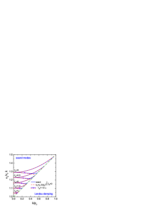
Figure 1: Spectrum of the sound modes defined by Eq. (23) for various values of the Landau parameters $f_{00}$ and $f_{02}$. Solid lines show the results of the numerical solution, dashed lines are the quadratic expansions with the parameters $s_{0}$ and $s_{2}$ given by Eqs. (27) and (29). The values of $f_{00}$ are shown in labels. Lines with (without) stars are calculated for $f_{02}=0$ ($f_{02}=-1.5\alpha$), where $\alpha$ is defined in Eq. (29). The dash-dotted line shows the border of the imaginary part of the Lindhard’s function (13). Below this line the frequency is complex.

The numerical solutions of Eq. (23) are shown in Fig. 1 by solid lines for various values of the Landau parameters $f_{00}$ and $f_{02}$. The zero-sound solution exists for $s_{0}>0$. We check that the inequality $1+f_{00}-s_{0}^{2}>0$ holds for $f_{00}>0$. The quadratic approximation for the spectrum $\omega\approx v_{\rm F}\,k\,[s_{0}+s_{2}x^{2}]$ is demonstrated by dashed lines. Only the quasi-particle part of the spectrum is shown with $\omega_{s}(k)/(v_{\rm F}\,k)>1+k/(2p_{\rm F})$. This inequality holds for $k/p_{{\rm F}}<k_{\rm max}/p_{\rm F}=(1-\sqrt{1-16s_{2}(s_{0}-1)})/(4\,s_{2})$ if $s_{2}\leq 1/[16(s_{0}-1)]$. For larger $k$ the Lindhard function becomes complex for continuation of the branch $\omega=\omega_{s}(k)$ and the solution of Eq. (23) acquires an imaginary part. For $s_{2}>1/[16(s_{0}-1)]$, the function $\omega_{s}(k)$ does not enter in the region of the complex Lindhard function. However, for positive $s_{2}$ there is another source of the mode dissipation related to the decay of one mode’s quantum in two quanta. The latter process is allowed if the energy-momentum relation $\omega_{s}(p)=\omega_{s}(p^{\prime})+\omega_{s}(|\vec{p}-\vec{p}{\,{}^{\prime}}|)$ holds, that is equivalent to the relation $1-\cos\phi=3s_{2}/(s_{0}p_{\rm F}^{2})$ , where $\cos\phi=(\vec{p}\,\vec{p}{\,{}^{\prime}})/(p\,p^{\prime})$, which is fulfilled if $s_{2}>0$.

In Fig. 1 we demonstrate first the case $f_{0}={\rm const}$, i.e., $f_{02}=0$. As we see, in this case $s_{2}>0$ for any $f_{00}>0$. We see that the quadratic approximation coincides very well with the full solution. Then we study how the spectrum changes if the parameter $f_{02}$ is taken nonzero. As we conclude from Eq. (29) the coefficient $s_{2}$ can be negative for $f_{02}<-\alpha\,.$ The latter implies: $f_{02}\stackrel{{\scriptstyle\scriptstyle<}}{{\phantom{}{}_{\sim}}}-10$ for $f_{00}=1$; $f_{02}\stackrel{{\scriptstyle\scriptstyle<}}{{\phantom{}{}_{\sim}}}-2.6$ for $f_{00}=2$; and $f_{02}\stackrel{{\scriptstyle\scriptstyle<}}{{\phantom{}{}_{\sim}}}-1.7$ for $f_{00}=3$. In Fig. 1 by solid curves and dashed curves marked with stars we depict the zero-sound spectrum for $f_{02}<-\alpha$, being computed following Eq. (23) and within the quadratic approximation, respectively. We chose here $f_{02}=-1.5\alpha$. The quadratic approximation for $s(x)$ works now worse for momenta close to $k_{\rm max}$ and the next term $s_{4}x^{4}$ should be included. We note that the parameter $s_{4}$ is positive in this case and the function $s(x)$ has a minimum at $x_{\rm min}=\sqrt{|s_{2}|/(2s_{4})}$. In the point $k=k_{0}$ corresponding to the minimum of $\omega_{s}(k)/k$ the group velocity of the excitation $v_{\rm gr}=d\omega_{s}/dk$ coincides with the phase one $v_{\rm ph}=\omega_{s}/k$. The quantity $\omega_{s}(k_{0})/k_{0}$ coincides with the value of the Landau critical velocity $u_{\rm L}$ for the production of Bose excitations in the superfluid moving with the velocity $u>u_{\rm L}$.

The effective vertex of the boson-fermion coupling (24) is shown in Fig. 2 as a function of $x$ for several values of $f_{00}$ and $f_{02}$. We plot it in the range $0<x<x_{\rm max}=k_{\rm max}/p_{\rm F}$, where the quasiparticle branch of the zero-sound spectrum is defined. For $f_{02}=0$ the vertex $V(k)$ is shown by solid lines, for $f_{02}<0$ by dash-dotted lines. We see that $V^{2}(x_{\rm max})$ is smaller for $f_{02}<0$ than for $f_{02}=0$. For small $x$ one can use the analytical expression

$$a^{2}N\frac{V^{2}(x)}{v_{\rm F}\,p_{\rm F}}=x\Big{[}\frac{\partial\Phi}{\partial s}\Big{|}_{s(x),x}\Big{]}^{-1}$$

$$\quad\approx\frac{s_{2}xf_{00}^{2}}{\alpha+f_{02}}\Big{[}1+\frac{4\alpha s_{2}x^{2}}{\alpha+f_{02}}\Big{(}6s_{2}-\frac{s_{0}}{s_{0}^{2}-1}\Big{)}\Big{]}\,,$$ (31)

which works well for $k\stackrel{{\scriptstyle\scriptstyle<}}{{\phantom{}{}_{\sim}}}0.75k_{\rm max}$. For $k\to 0$ we get $a^{2}N{V^{2}(k)}\simeq s_{0}(s_{0}^{2}-1)^{2}f_{00}kv_{{\rm F}}/(1+f_{00}-s_{0}^{2})$.

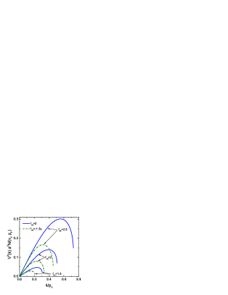
Figure 2: Coupling constant of zero-sound modes and fermions as a function of the momentum $k$ for various values of the Landau parameters $f_{00}$ and $f_{02}$, calculated from Eq. (24). All curves end at the limiting value of $x_{\rm max}=k_{\rm max}/p_{\rm F}$ at which the spectral branch enters into the region of complexity of the $\Phi$ function.

II.3 Moderate attraction, $-1<f_{00}<0$. Diffusons.

Assume $f_{02}=0$. For $-1<f_{00}<0$, Eq. (23) has only damped solutions with $\Re s<1$ and $\Im s<0$. In the limit of $s,x\ll 1$, using the expansion (20) we easily find the analytic solution

$$\frac{\omega_{\rm d}(k)}{kv_{\rm F}}=is_{\rm d}(x)\approx-i\frac{2}{\pi}\left[\frac{1-|f_{00}|}{|f_{00}|}+\frac{x^{2}}{12}\right]\,,$$ (32)

which is valid for $1-|f_{00}|\ll 1$ and $x\ll 1$. We see that the solution we found is purely imaginary and its dependence on $x$ is very weak.

More generally, for purely imaginary $s=i\,\tilde{s}$, $\tilde{s}\in R$, the Lindhard function can be rewritten as

$$\Phi(i\tilde{s},x)=\widetilde{\Phi}(\tilde{s},x)=\frac{1}{4x}\big{[}\tilde{s}^{2}-{\textstyle\frac{1}{4}}x^{2}+1\big{]}\log\frac{\tilde{s}^{2}+\left({\textstyle\frac{1}{2}}x+1\right)^{2}}{\tilde{s}^{2}+\left({\textstyle\frac{1}{2}}x-1\right)^{2}}$$

$$\quad+\frac{{\tilde{s}}}{2}\left[{\rm arctan}\frac{\tilde{s}}{1-{\textstyle\frac{1}{2}}x}+{\rm arctan}\frac{\tilde{s}}{1+{\textstyle\frac{1}{2}}x}\right]+\frac{1-\pi\tilde{s}}{2}\,.$$ (33)

We note that the function ${\rm arctan}(\tilde{s}/[1-{\textstyle\frac{1}{2}}x])$ should be continuously extended for $x>2$ as ${\rm arctan}(\tilde{s}/[1-{\textstyle\frac{1}{2}}x])+\pi{\rm sign}\tilde{s}$ . Solutions of equation

$$1/|f_{00}|=\Phi(i\tilde{s},x)$$ (34)

for $0>f_{00}>-1$ are depicted in Fig. 3 for $f_{00}=-0.2;-0.5;-0.9$. These solutions are damped ($-i\omega<0$). For $f_{02}\neq 0$ (at the condition $0>f_{0}(k)>-1$), the damped character of the solutions does not change.

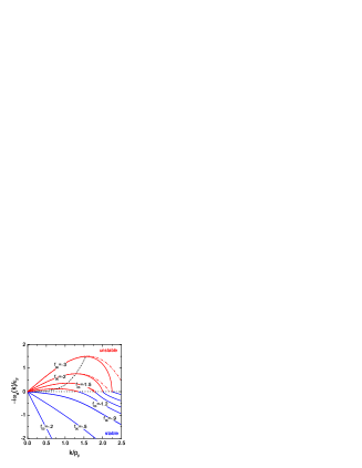
Figure 3: Solid lines show the purely imaginary solutions of Eq. (34) for various values of the Landau parameter $f_{00}<0$. Dashed line indicates positions of the maxima of spectra $\omega_{\rm d}$ for $f_{00}<-1$. Dash-dotted lines show the approximated spectra $\omega_{\rm d}(k)\approx iv_{\rm F}k(s_{\rm d0}+s_{\rm d2}\,x^{2}+s_{\rm d4}x^{4})$ with the parameters from Eqs. (37) and (38).

II.4 Strong attraction, $f_{00}<-1$. Pomeranchuk instability.

Now we consider the case of a strong attraction in the scalar channel $f_{00}<-1$. We continue to assume $f_{02}=0$ for certainty. The Pomeranchuk instability for $f_{00}<-1$ manifests itself in the negative compressibility which is found from the relation for the variation of the fermion contribution to the chemical potential LP1981

$$K=\frac{p^{2}_{{\rm F}}(n_{0})}{3m_{{\rm F}}^{*}(n_{0})}(1+f_{00})\,,$$ (35)

being negative for $f_{00}<-1$.

Solutions of Eq. (34) for $f_{00}<-1$ are shown in Fig. 3. We see that there is an interval of $k$, $0<k<k_{\rm d}$, where $-i\omega_{\rm d}>0$ and, hence, the mode is exponentially growing with time. This corresponds to the Pomeranchuk instability in a Fermi system with strong scalar attraction, see Ref. Nozieres . For $k>k_{\rm d}$ we get $-i\omega_{\rm d}(k>k_{\rm d})<0$, and the mode becomes stable again. The momentum $k_{\rm d}$ is determined from Eq. (34) for $\tilde{s}=0$:

$$\frac{1}{f_{00}}=\frac{x_{\rm d}^{2}-4}{8x_{\rm d}}\log\left|\frac{x_{\rm d}+2}{x_{\rm d}-2}\right|-\frac{1}{2}\,,$$ (36)

$x_{\rm d}=k_{\rm d}/p_{\rm F}$. The instability increment $-i\omega_{\rm d}$ has a maximum at some momentum $k_{m}$. The locations of maxima for different $f_{00}$ values are connected by dashed line in Fig. 3.

The spectrum of the unstable mode can be written for $x<<1$ as $s_{\rm d}(x)\approx s_{\rm d0}+s_{\rm d2}x^{2}+s_{\rm d4}\,x^{4}$, where the leading term is determined by the equation

$$\frac{\pi}{2}-\arctan s_{\rm d0}=\frac{z_{f}}{s_{\rm d0}}\,,\quad z_{f}=1-1/|f_{00}|\,.$$ (37)

The subleading terms are equal to

$$s_{\rm d2} =\frac{s_{\rm d0}}{12(1+s_{\rm d0}^{2})(z_{f}\,(1+s_{\rm d0}^{2})-s_{\rm d0}^{2})}\,,$$

$$s_{\rm d4} =\frac{1-5s_{\rm d0}^{2}}{20(1+s_{\rm d0}^{2})^{2}}s_{\rm d2}-\frac{4s_{\rm d0}s_{\rm d2}^{2}}{1+s_{\rm d0}^{2}}-12s_{\rm d2}^{2}\,.$$ (38)

This approximation of the spectrum is illustrated in Fig. 3 by dash-dotted lines. The approximation works very well for $-1.5<f_{00}<-1$ (dash-dotted lines and solid lines coincide) but becomes worse for smaller $f_{00}$.

For a slightly subcritical case, where $0<z_{f}\ll 1$, we obtain

$$\omega_{\rm d}(k)\approx i\frac{2}{\pi}v_{\rm F}k\,[z_{f}-k^{2}/(12p_{\rm F}^{2})]\,.$$ (39)

The function $-i\omega_{\rm d}$ has a maximum at $k_{m}=2p_{\rm F}\sqrt{z_{f}}$ equal to

$$-i\omega_{m}=({8}/{3\pi})v_{\rm F}p_{\rm F}\,z_{f}^{3/2}\,.$$ (40)

II.5 Spinodal instability.

For $f_{00}<-1$ not only the compressibility is negative but also the square of the first sound velocity  LP1981

$$u^{2}=\frac{\partial P}{\partial\rho}=\frac{p_{\rm F}^{2}}{3m_{\rm F}m^{*}_{\rm F}}(1+f_{00})<0\,.$$ (41)

Here $P$ denotes the pressure and $\rho$ is the mass density. Note that in the limit $T\to 0$ the isothermal and adiabatic compressibilities coincide, whereas for $T\neq 0$ the difference becomes substantial, see Ref. VS:2010gf . Also note that the first sound exists in the hydrodynamical (collisional) regime, i.e. for $\omega\ll\tau_{\rm col}^{-1}\propto T^{2}$, which is the opposite limit to the collision-less regime of the zero sound, i.e. $\omega\gg\tau_{\rm col}^{-1}$.

For the van der Waals equation of state the compressibility and the square of the first sound velocity prove to be negative in the spinodal region. Thereby excitation spectrum is unstable and in simplest case of ideal hydrodynamics the growing mode is as follows VS:2010gf

$$-i\omega=k\sqrt{|u^{2}-ck^{2}|}\,,$$ (42)

where $c$ is a coefficient associated with the surface tension of the droplets of one phase in the other one. Note that the viscosity and thermal conductivity may delay formation of the hydrodynamic modes. Maximum in $k$ yields

$$-i\omega_{m}=v_{\rm F}p_{\rm F}(|f_{00}|-1)/(6m_{\rm F}\sqrt{c})\,.$$ (43)

The rate of the growing of the spinodal mode decreases with increase of the surface tension of the droplets, whereas the growing rate of the collision-less mode does not depend on the surface tension. For

$$c>\frac{\pi^{2}|f_{00}|^{3/2}}{256m_{\rm F}^{2}(|f_{00}|-1)}$$ (44)

the zero-sound-like excitations (39) would grow more rapidly than excitations of the ideal hydrodynamic mode (43).

For isospin symmetric nuclear matter the spinodal region in the dependence $P(1/n)$ exists at nucleon densities below the saturation nuclear density, see Ref. SVB . In multi component systems with charged constituents, like neutron stars, the resulting stationary state is the mixed pasta state, where finite size effects (surface tension and the charge screening) are very important, cf. Refs. Maruyama:2005vb ; Tatsumi:2002dq , contrary to the case of the one component system, where the stationary state is determined by the Maxwell construction, cf. Ref. SVB . The liquid-gas phase transition may occur in heavy-ion collisions. A nuclear fireball prepared in a course of collision has a rather small size, typically less or of the order of the Debye screening length. Therefore, the pasta phase is not formed, as in a one-component system.

III Bosonization of the local interaction

The description of a fermionic system with a contact interaction can be equivalently described in terms of bosonic fields $\phi_{q}=\sum_{p}\psi^{\dagger}_{p}\psi_{p+q}$, here we denote $q=(\omega,\vec{k})$ and $p=(\epsilon,\vec{p})$. In terms of the functional path integral the transition to the collective bosonic fields can be performed with the help of a formal change of variables by means of a Hubbard-Stratonovich transformation Altland-Simons ; Kopietz . After this transformation the effective Euclidean action for the system with a repulsive interaction, here $f_{0}>0$, can be written within the Matzubara technique in terms of the bosonic fields as

$$S[\phi]=\sum_{q}\frac{\phi_{q}\,\phi_{-q}}{2\Gamma_{0}^{\omega}}-\operatorname{Tr}\log\Big{[}1-\frac{\hat{G}i\hat{\phi}_{q}}{\beta}\,\Big{]}\,,$$ (45)

where $\hat{G}$ and $\hat{\phi}$ are infinite matrices in frequency/momentum space with matrix elements $[\hat{G}]_{p,p^{\prime}}=\delta_{p,p^{\prime}}G(\epsilon,\vec{p}\,)$ and $[\hat{\phi}]_{q,q^{\prime}}=\delta_{q,q^{\prime}}\phi_{\vec{q}}$. Trace is taken over frequencies and momenta and includes factor 2 accounting for the fermion spins. Transformation to zero temperature follows by the standard replacement $\beta^{-1}\sum_{n}\to\int d\epsilon/(2\pi i)$.

Expanding Eq. (45) up to the 4-th order in $\phi$ for $T=0$ we obtain

$$S[\phi]\approx\frac{1}{2}\mbox{sgn}(f_{0})\sum_{q}\phi_{q}\,\big{(}(\Gamma_{0}^{\omega})^{-1}+a^{2}N\Phi(s,x)\big{)}\phi_{-q}$$ (46)

$$\qquad+\frac{1}{4}\sum_{\{q_{i}\}}U(q_{1},q_{2},q_{3},q_{4})\phi_{q_{1}}\phi_{q_{2}}\phi_{q_{3}}\phi_{q_{4}}\delta_{q_{1}+q_{2}+q_{3}+q_{4},0}\,,$$

where the effective field self–interaction is given by the function

$$U(q_{1},q_{2},q_{3},q_{4}) =-2i\frac{1}{4!}\sum_{\mathcal{P}(1,\dots,4)}\sum_{p}G_{p}G_{p+q_{1}}$$

$$\times G_{p+q_{1}+q_{2}}G_{p+q_{1}+q_{2}+q_{3}}\,.$$ (47)

Here the sum $\sum_{\mathcal{P}}$ runs over the $4\!$ permutations of $4$ momenta $q_{i}$. As we will show, Eq. (46) is applicable also for $f_{0}<0$ after the replacement $\phi\to i\phi$ that results in the appearance of the prefactor $\mbox{sgn}(f_{0})$ in Eq. (46).

The general analysis of Eq. (46) for arbitrary external momenta was undertaken in Ref. Brovman . The first term in Eq. (46) (quadratic in $\phi$) can be interpreted as the inversed retarded propagator of the effective boson zero-sound-like mode:

$$(D^{R}_{\phi})^{-1}(\omega,k)=-{\rm sgn}(f_{0})[(\Gamma_{0}^{\omega})^{-1}+a^{2}N\Phi(s,x)]\,.$$ (48)

To describe modes for an attractive interaction, $f_{0}<0$, it is instructive to re-derive the expression for the mode propagator using the approach proposed in Ref. IKV00 . The local four-fermion interaction $\Gamma_{0}^{\omega}$ can be viewed as an interaction induced by the exchange of a scalar heavy boson with the mass $m_{\rm B}$,

$$\Gamma_{0}^{\omega}\to-\frac{\Gamma_{0}^{\omega}m_{\rm B}^{2}}{(\omega+i0)^{2}-k^{2}-m_{B}^{2}}\equiv-\Gamma_{0}^{\omega}\,m_{\rm B}^{2}\,D^{R}_{\rm B,0}(\omega,k)\,,$$ (49)

where $D^{R}_{\rm B,0}$ is the bare retarded Green’s function of the heavy boson and we assumed that $m_{\rm B}^{2}$ is much larger then typical squared frequencies and momenta, $\omega^{2},k^{2}$, in the problem.

Then making the replacement (49) in the fermion scattering amplitude (11) we obtain

$$T^{R}_{{\rm ph},0}(\omega,k) =\frac{-(a^{2}N)^{-1}f_{0}m_{\rm B}^{2}}{(D_{{\rm B},0}^{R})^{-1}(\omega,k)-\Sigma^{R}_{\rm B}(\omega,k)}\equiv V_{\rm B}^{2}D^{\rm R}_{\rm B}(\omega,k)\,.$$ (50)

Hence, we can identify the vertex of the boson-fermion interaction

$$V_{\rm B}^{2}=-f_{0}m_{\rm B}^{2}/(a^{2}N)\,,$$ (51)

and the full retarded Green’s function of the boson $D^{R}_{\rm B}(\omega,k)$ with the retarded self-energy

$$\Sigma^{R}_{\rm B}(\omega,k)=f_{0}m_{\rm B}^{2}\Phi\big{(}\frac{\omega}{kv_{\rm F}},\frac{k}{p_{\rm F}}\big{)}\,.$$ (52)

Note that for very large $m_{\rm B}$ that we have assumed, $D^{\rm R}_{\rm B}(\omega,k)$ in (50) differs from $D^{\rm R}_{\phi}(\omega,k)$ in (48) only by a prefactor. For the attractive interaction, which we are now interested in ($f_{0}<0$), we have $m_{\rm B}^{2}>0$ and $V_{\rm B}^{2}>0$. For repulsive interaction instead of the bare scalar boson the bare vector boson would be an appropriate choice, cf.  IKV00 , or we may come back to the formalism given by Eqs. (45) – (47).

The spectrum follows from the solution of the Dyson equation $0=[D_{\rm B}^{R}(\omega,k)]^{-1}\approx-m_{\rm B}^{2}(1+f_{0}\Phi(s,x))$ for $m_{\rm B}\gg\omega,k$ and coincides with the solution of Eq. (23). The boson spectral function is given by

$$A_{\rm B}(\omega,k)=-2\Im D_{\rm B}^{R}(\omega,k),$$

$$-2\Im T^{R}_{{\rm ph},0}(\omega,k)=V_{\rm B}^{2}A_{\rm B}(\omega,k)\,.$$ (53)

IV Avoiding of the Pomeranchuk instability by a Bose condensation

IV.1 Condensation of a scalar field for $f_{0}<-1.$

Consider a Fermi liquid with local scalar interaction $f_{0}<-1$. We assume that the bosonization procedure of the interaction, Eqs. (49) and (50), is performed. According to the perturbative analysis in Sect. II.4, for $f_{0}<-1$ there are modes which grow with time. The growth of hydrodynamic modes (first sound), cf. Eqs. (42) and (43), results in the formation of a mixed phase. Besides the hydrodynamic modes the zero-sound-like modes grow with time, cf. Eqs. (39) and (40). We study now the opportunity that the instability of the zero-sound mode may result in a formation of a static condensate of the scalar field. This leads to a decrease of the system energy and to a rearrangement of the excitation spectrum on the ground of the condensate field.

We will exploit the simplest probing function describing the complex scalar field of the form of a running wave

$$\varphi=\varphi_{0}e^{-i\omega_{c}t+i\vec{k}_{c}\vec{r}}\,,$$ (54)

with the condensate frequency and momentum $(\omega_{c},\vec{k}_{c})$ and the constant amplitude $\varphi_{0}$. The choice of the structure of the order parameter is unimportant for our study of the stability of the system.

Guided by the construction of the full Green’s function of the effective boson field, see Eq. (50), the effective Lagrangian density for the condensed field (54) can be written as, cf. Ref. MSTV90 ; V84 ,

$$L=\Re D_{\rm B}^{-1}(\omega_{c},k_{c})|\varphi_{0}|^{2}-{\textstyle\frac{1}{2}}V_{\rm B}^{4}\Lambda(\omega_{c},k_{c})|\varphi_{0}|^{4}\,.$$ (55)

The energy density of the condensate is given then by the standard relation

$$E_{\rm B}=\omega\partial L/\partial\omega-L\,.$$

Fully equivalently, this Lagrangian density can be written in the form suggested by expansion (46), now applied for the running wave classical field, after the field redefinition $m_{\rm B}\varphi_{0}=a\sqrt{N/|f_{0}|}\phi_{0}$,

$$L=\Re D_{\phi}^{-1}(\omega_{c},k_{c})|\phi_{0}|^{2}-{\textstyle\frac{1}{2}}\Lambda(\omega_{c},k_{c})|\phi_{0}|^{4}\,.$$ (56)

Here and in Eq. (55) the quantity $\Lambda(\omega_{c},k_{c})$ represents the self-interaction amplitude of condensed modes which corresponds to the ring diagram with four fermion Green’s functions (47), $\Lambda(\omega_{c},k_{c})=6U(q_{c},-q_{c},q_{c},-q_{c})$. As we shall see below the energetically favorable is the state with $\omega_{c}=0$, and therefore we put $\omega_{c}=0$ here. The leading order contribution to the self-interaction parameter $\Lambda(0,k_{c})$ as a function of the condensate momentum was calculated in Ref. Brovman :

$$\Lambda(0,k_{c}) =\frac{8a^{4}}{\pi^{2}v_{\rm F}^{3}x_{c}^{4}}\Big{[}\frac{1-x_{c}^{2}}{x_{c}}\ln\Big{|}\frac{2+x_{c}}{2-x_{c}}\Big{|}-\frac{1-x_{c}^{2}}{2x_{c}}\ln\Big{|}\frac{1+x_{c}}{1-x_{c}}\Big{|}$$

$$+\frac{x_{c}^{2}}{4-x_{c}^{2}}\Big{]}\,,\quad x_{c}=k_{c}/p_{\rm F}.$$ (57)

For $x_{c}\ll 1$ we get

$$\Lambda(0,k_{c})\approx a^{4}\lambda\,\Big{(}1+\frac{k_{c}^{2}}{2p_{\rm F}^{2}}\Big{)}\,,\quad\lambda=\frac{1}{\pi^{2}v_{\rm F}^{3}}\,.$$ (58)

The quantity $\lambda$ agrees also with the result derived in Ref. D82 for description of the pion condensation in the Thomas-Fermi approximation.

The equation of motion for the field amplitude follows from the variation of the action corresponding to the Lagrangian density (56),

$$-a^{2}N\tilde{\omega}^{2}(k_{c})\phi_{0}-\Lambda(0,k_{c})\,|\phi_{0}|^{2}\phi_{0}=0\,,$$ (59)

where we introduce the effective boson gap

$$\tilde{\omega}^{2}(k_{c})=[1-|f_{0}(k_{c})|\Phi(0,k_{c})]/|f_{0}(k_{c})|\,,$$ (60)

as it was done in the description of the pion condensation, see Ref. MSTV90 . The equation for the condensate amplitude (59) has a non trivial solution for $\tilde{\omega}^{2}(k_{c})<0$,

$$|\phi_{0}|^{2}=-N\frac{\tilde{\omega}^{2}(k_{c})}{a^{2}\lambda\,\Big{(}1+\frac{k_{c}^{2}}{2p_{\rm F}^{2}}\Big{)}}\,\theta(-\tilde{\omega}^{2}(k_{c}))\,,$$ (61)

which corresponds to the gain in the energy density

$$E_{\rm B}=-N^{2}\frac{\tilde{\omega}^{4}(k_{c})}{2\lambda\,\Big{(}1+\frac{k_{c}^{2}}{2p_{\rm F}^{2}}\Big{)}}\theta(-\tilde{\omega}^{2}(k_{c}))\,,$$ (62)

where $\theta(x)=1$ for $x>0$ and 0 otherwise.

IV.2 Bose condensation in a homogeneous state.

If the minimum of the gap $\tilde{\omega}^{2}$ is realized at $k_{c}=0$, e.g., it is so for $f_{02}\geq 0$, the energy density $E_{\rm B}$ is minimized for $\omega_{c}=k_{c}=0$. Then, the field amplitude and the condensate energy density are

$$\phi_{0}^{2}=N\frac{z_{f}}{a^{2}\lambda}\,\theta(z_{f})\,,\quad E_{\rm B}=-N^{2}\frac{z_{f}^{2}}{2\lambda}\,\theta(z_{f})\,,$$ (63)

where we used the same notation $z_{f}$ as in Eq. (37). The Bose condensate is formed for $f_{00}<-1$.

For the case of non-zero temperature, $T\neq 0$, in the mean field approximation one should just replace $\Phi\to\Phi_{T}$, where the fermion step-function distributions are replaced to the thermal distributions, and from Eq. (21) for $T\ll\epsilon_{\rm F}$ one recovers the critical temperature of the condensation $T^{\rm MF}/\epsilon_{\rm F}=\sqrt{12\,z_{f}}/\pi$ valid for $0<z_{f}\ll 1$. For $|f_{00}|\gg 1$ from Eq. (22) one gets $T^{\rm MF}/\epsilon_{\rm F}=2|f_{00}|/3$ .

In the presence of the homogeneous condensate ($k_{c}=0$) setting $\phi_{q}=\phi_{0}+\phi^{\prime}_{q}$ in (46), (56), varying in $\phi^{\prime}_{q}$ and retaining only terms linear in $\phi^{\prime}_{q}$ we recover the spectrum of overcondensate excitations

$$a^{2}N\Big{[}-|f_{00}|^{-1}+\Phi\Big{(}\frac{\omega}{v_{\rm F}k},\frac{k}{p_{\rm F}}\Big{)}\Big{]}-\delta\Sigma_{\varphi}=0,$$ (64)

where the last term arises from the interaction of excitations with the condensate. Making use of Eqs (20), (58), and (63) we find

$$\delta\Sigma_{\varphi}=2\,a^{2}N\,z_{f}+O(\omega^{2},k^{2},\omega/k\to 0)$$ (65)

and derive the spectrum for $z_{f}\ll 1$ and $x\ll 1$,

$$\tilde{\omega}\approx-i\frac{2}{\pi}z_{f}kv_{\rm F}\,.$$ (66)

So, the overcondensate excitations are damped, similar to those we obtain for the case $-1<f_{00}<0$, see Eq. (32).

In the presence of the condensate ($f_{00}<-1$) the particle-hole interaction is described by scattering amplitude

$$a^{2}\,N\,T_{\rm ph,0}^{R}=\Big{[}\frac{1}{f_{0}}+\Phi-\frac{\delta\Sigma_{\varphi}}{a^{2}N}\Big{]}^{-1}$$

$$\simeq\Big{[}\frac{1}{f_{\rm ren,0}}+1+i\frac{\pi\omega}{2kv_{\rm F}}+O(\omega^{2},k^{2},\omega/k\to 0)\Big{]}^{-1}\,,$$ (67)

where in the second equality we introduce the renormalized local interaction

$$f_{\rm ren,0}\approx f_{\rm ren,00}=-\frac{f_{00}}{2f_{00}+1}\,.$$ (68)

The latter equation shows that if originally we have $f_{00}<-1$, the renormalized interaction $-1<f_{\rm ren,00}<-1/2$. Thus, in the presence of the boson condensate the Fermi liquid is free from the Pomeranchuk instability.

Using the renormalized parameter $f_{\rm ren,00}$ we can calculate how the fermion chemical potential changes in the presence of the condensate. We use here the standard expression from Ref. M67 for the variation of the chemical potential with the particle density in the Fermi liquid theory

$$\delta\mu_{\rm F}=\frac{2\epsilon_{{{\rm F}},0}}{3n_{0}}\delta n+\frac{f_{\rm ren,00}}{N}\delta n\,,$$ (69)

here $\epsilon_{{{\rm F}},0}=p_{\rm F}^{2}(n_{0})/2m^{*}_{\rm F}(n_{0})$. The energy density can be obtained from the relation $E=\int_{0}^{\mu_{\rm F}}\mu_{\rm F}dn$.

The compressibility of the system becomes now

$$K =n_{0}\frac{\delta\mu_{\rm F}}{\delta n}\Big{|}_{n_{0}}+K_{\rm B}$$

$$=\frac{p^{2}_{\rm F}(n_{0})}{3m_{\rm F}^{*}(n_{0})}\big{(}1+f_{\rm ren,00}\big{)}+K_{\rm B}\,,$$ (70)

where the first term in the second line is always positive

$$1+f_{\rm ren,00}=(|f_{00}|-1)/(2|f_{00}|-1)>0\,,$$ (71)

for $f_{00}<-1$ under consideration. The second term is the condensate term:

$$K_{\rm B}=n_{0}\frac{d^{2}E_{\rm B}}{dn^{2}}\Big{|}_{n_{0}}\,.$$ (72)

Similarly, the square of the first sound velocity in the presence of the condensate becomes

$$u^{2}=\frac{\partial P}{\partial\rho}=\frac{p_{\rm F}^{2}}{3m_{\rm F}m^{*}_{\rm F}}(1+f_{\rm ren,00})>0\,,$$ (73)

whereas in the absence of the condensate it was $\propto(1+f_{00})<0$, cf. Eq. (41).

Recall that $u^{2}$ is negative within the spinodal region which exists, if the pressure has a van-der-Waals form. Thus, the formation of the scalar Bose condensate, suggested here, might compete with the development of the spinodal instability at the liquid-gas phase transition in Fermi liquids. From general principles, one can expect that the system will develop a (stable or metastable) condensate state at least, if a surface tension between liquid and gas regions is sufficiently high. Then aerosol-like mixture appearing in the course of the development of the spinodal decomposition will evolve more slowly compared to the process of the formation of the scalar condensate.

IV.3 Bose condensation in an inhomogeneous state.

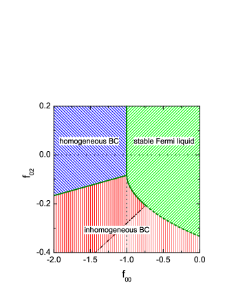
Figure 4: Phase diagram of a Fermi liquid with a scalar interaction in the particle hole channel described by the momentum dependent coupling constant $f_{0}(k/p_{\rm F})=f_{00}+f_{02}k^{2}/p_{\rm F}^{2}$. Depending on the values of parameters $f_{00}$ and $f_{02}$ the Fermi liquid can be either in a stable state or in states with homogeneous or inhomogeneous static Bose condensates (BC) of scalar modes. Possibility of the development of the spinodal instability is suppressed.

We discuss now how the momentum dependence of the coupling constant $f_{0}$, as given by Eq. (26), may influence the condensation of the scalar mode. The condition for the appearance of a condensate with $\omega_{c}=0$ and a finite momentum $k_{c}$ are determined by relations $\tilde{\omega}^{2}(k_{c})\leq 0\,,\quad\frac{{\rm d}}{{\rm d}k}\tilde{\omega}^{2}(k_{c})=0$ . The critical condition for the appearance of the condensate can be deduced from the expansion of $|f_{0}|\tilde{\omega}^{2}(k)$ in (60) for $x^{2}\sim x_{m}^{2}$:

$$1+f_{0}(x)\Phi(0,x)\approx 1+f_{00}+3\frac{(f_{02}-\frac{f_{00}}{12})^{2}}{(f_{02}+\frac{f_{00}}{20})}$$

$$-\frac{f_{02}+\frac{f_{00}}{20}}{12}[x^{2}-x_{m}^{2}]^{2}\,,\quad x_{m}^{2}=6\frac{f_{02}-\frac{f_{00}}{12}}{f_{02}+\frac{f_{00}}{20}}.$$ (74)

For $f_{00}<-1$ this function has always a negative minimum at $x=0$, the second and deeper minimum appears at finite $x$, if

$$f_{02}\leq f_{02}^{\rm cr}={f_{00}}/{12}\,.$$ (75)

For $-1<f_{00}<0$ the minimum at finite momentum can be realized if

$$f_{02}\leq f_{02}^{\rm cr}=-\frac{1}{6}\Big{[}1+{\textstyle\frac{1}{2}}f_{00}+\sqrt{1+\frac{2}{5}f_{00}-\frac{3}{5}f_{00}^{2}}\Big{]}\,,$$ (76)

and

$$x_{m}^{2}(f_{02}^{\rm cr})=6\frac{1+f_{00}+\sqrt{1+\frac{2}{5}f_{00}-\frac{3}{5}f_{00}^{2}}}{1+\sqrt{1+\frac{2}{5}f_{00}-\frac{3}{5}f_{00}^{2}}+\frac{1}{5}f_{00}}\,.$$ (77)

The solid lines in Fig. 4 on the $(f_{00},f_{02})$ plane show the critical values $f_{02}^{\rm cr}$ given by Eqs. (75) and (76). They form the phase diagram of the Fermi liquid with the momentum dependent interaction in the scalar channel. The dash-dotted line shows solution of equation $f_{02}x_{m}^{2}=f_{00}$. In the region restricted by this dash-dotted line and the dash continuation of the solid line we have $|f_{00}|<|f_{02}|x_{m}^{2}$ and the expansion (26) for $f_{0}(k)$ becomes questionable.

Near the minimum the boson gap $\tilde{\omega}^{2}(k)$ can be presented as

$$\tilde{\omega}^{2}(k)=\tilde{\omega}^{2}_{0}(k_{c})+\frac{\gamma}{4k_{c}^{2}}(k^{2}-k_{c}^{2})^{2}\,,$$ (78)

for $\gamma={\rm const}$. The critical point is found from the condition $\tilde{\omega}^{2}_{0}(k_{c}=k_{\rm cr})=0$. Beyond the critical point the actual value of $k_{c}$ follows from the minimum of the energy density (62) as a function of $k_{c}$.

V Condensate of Bose excitations with non-zero momentum in a moving Fermi liquid

Let us apply the constructed above formalism to the analysis of a possibility of condensation of zero-sound-like excitations with a non-zero momentum and frequency in a moving Fermi liquid. The main idea was formulated in Refs. Pitaev84 ; V93 ; Vexp95 ; Melnikovsky ; BP12 ; KV2015 ; Kolomeitsev:2015dua . When a medium moves in straight line with the velocity $u>u_{\rm L}={\rm min}[\omega(k)/k]$ (where the minimum is realized at $k=k_{0}\neq 0$), it may become energetically favorable to transfer a part of the momentum from the particles of the moving medium to a condensate of collective Bose excitations with the momentum $k_{0}$. The condensation may occur, if in the spectrum branch $\omega(k)$ there is a region with a small energy at sufficiently large momenta.

As in Ref. V93 , we consider a fluid element of the medium with the mass density $\rho$ moving with a non-relativistic constant velocity $\vec{u}$. The quasiparticle energy $\omega(k)$ in the rest frame of the fluid is determined from the dispersion relation

$$\Re D_{\phi}^{-1}(\omega,k)=0\,.$$ (79)

We continue to exploit the complex scalar condensate field described by the simplest running-wave probing function, cf. Eq. (54), and the Lagrangian density (56), but now for the condensate of excitations.

The appearance of the condensate with a finite momentum $\vec{k}_{0}$, frequency $\omega=\omega(k_{0})$ and an amplitude $\varphi_{0}$ leads to a change of the fluid velocity from $\vec{u}$ to $\vec{u}_{\rm fin}$, as it is required by the momentum conservation

$$\rho\vec{u}=\rho\vec{u}_{\rm fin}+\vec{k}_{0}Z^{-1}_{0}|\phi_{0}^{2}|\,,$$ (80)

where $\vec{k}_{0}Z^{-1}_{0}|\phi_{0}^{2}|$ is the density of the momentum of the condensate of the boson quasiparticles with the quasiparticle weight

$$Z^{-1}_{0}(k_{0})=\Big{[}\frac{\partial}{\partial\omega}\Re D^{-1}_{\phi}(\omega,k)\Big{]}_{\omega(k_{0}),k_{0}}>0\,.$$ (81)

If in the absence of the condensate of excitations the energy density of the liquid element was $E_{\rm in}=\rho u^{2}/2$, then in the presence of the condensate of excitations, which takes a part of the momentum, the energy density becomes

$$E_{\rm fin}={\textstyle\frac{1}{2}}\rho u_{\rm fin}^{2}+\omega(k_{0})Z^{-1}_{0}|\phi_{0}|^{2}+{\textstyle\frac{1}{2}}\Lambda(\omega(k_{0}),k_{0})|\phi_{0}|^{4}.$$ (82)

Here the last two terms appear because of the classical field of the condensate of excitations. The gain in the energy density due to the condensation, $\delta E=E_{\rm fin}-E_{\rm in}$, is equal to

$$\delta E=-[\vec{u}\vec{k}_{0}-\omega(k_{0})]\,Z^{-1}_{0}(k_{0})\,|\phi_{0}|^{2}+{\textstyle\frac{1}{2}}\widetilde{\Lambda}|\phi_{0}|^{4}\,,$$ (83)

where

$$\widetilde{\Lambda}=\Lambda(\omega(k_{0}),k_{0})+(Z^{-1}_{0}(k_{0}))^{2}k_{0}^{2}/\rho\,.$$ (84)

For $\omega=0$, $\Lambda(0,k_{0})$ is calculated explicitly, cf. Eq. (58). Note that above equations hold also for $\Lambda=0$.

The condensate of excitations is generated for the velocity of the medium exceeding the Landau critical velocity, $u>u_{\rm L}=\omega(k_{0})/k_{0}$, where the direction of the condensate vector $\vec{k}_{0}$ coincides with the direction of the velocity, $\vec{k_{0}}\parallel\vec{u}$, and the magnitude $k_{0}$ is determined by the equation $\omega(k_{0})/k_{0}={\rm d}\omega(k_{0})/{\rm d}k$. The gain in the energy density after the formation of the classical condensate field with the amplitude $\phi_{0}$ and the momentum $k_{0}$ is then

$$\delta E=-Z^{-1}_{0}(k_{0})[uk_{0}-\omega(k_{0})]\phi_{0}^{2}+{\textstyle\frac{1}{2}}\widetilde{\Lambda}\phi_{0}^{4}\,.$$ (85)

The amplitude of the condensate field is found by minimization of the energy. From (85) one gets

$$\phi_{0}^{2}=Z^{-1}_{0}(k_{0})\frac{uk_{0}-\omega(k_{0})}{\widetilde{\Lambda}}\theta(u-u_{c})\,.$$ (86)

The resulting velocity of the medium becomes

$$u_{\rm fin}=u_{c}+\frac{(u-u_{c})\theta(u-u_{c})}{1+[Z^{-1}_{0}(k_{0})]^{2}k_{0}^{2}/(\Lambda(\omega(k_{0}),k_{0})\rho})\,.$$ (87)

For a small $\Lambda$, we have $u_{\rm fin}=u_{c}+O(\Lambda)$.

For the repulsive interaction $f_{0}>0$ there is real zero-sound branch of excitations $\omega_{\rm s}(k)\approx kv_{\rm F}(s_{0}+s_{2}\,x^{2}+s_{4}\,x^{4})$, where the parameters $s_{i}$ depend on the coupling constants $f_{00}$ and $f_{02}$ according to Eqs. (27), (29), and (30). As shown in Sect. II.2 the ratio $\omega_{\rm s}(k)/(kv_{\rm F})$ has a minimum at $k_{0}=p_{\rm F}\sqrt{-s_{2}/(2s_{4})}$ provided $f_{02}$ is smaller than $f_{\rm crit,02}=-f_{00}^{2}/[12(s_{0}^{2}-1)^{2}]$. The Landau critical velocity of the medium is equal to $u_{\rm L}/v_{\rm F}=\omega_{\rm s}(k_{0})/(v_{\rm F}k_{0})\approx s_{0}-s_{2}^{2}/(2s_{4})$. The quasiparticle weight of the zero-sound mode (81) is

$$Z_{0}^{-1}(k_{0})=\frac{a^{2}N}{k_{0}v_{\rm F}}\frac{\partial\Phi(s,x)}{\partial s}\Big{|}_{\frac{\omega_{s}(k_{0})}{v_{\rm F}k_{0}},\frac{k_{0}}{p_{\rm F}}}\,.$$ (88)

The amplitude of the condensate field (86) can be written as

$$\varphi^{2}_{0}=Z_{0}^{-1}(k_{0})k_{0}\frac{u-u_{\rm L}}{\widetilde{\Lambda}}\theta(u-u_{\rm L})\,.$$ (89)

The energy density gained owing to the condensation of the excitations is

$$\delta E=-k_{0}^{2}(Z^{-1}_{0}(k_{0}))^{2}\frac{(u-u_{\rm L})^{2}}{2\widetilde{\Lambda}}\theta(u-u_{\rm L})\,.$$ (90)

For a small $\lambda$, Eqs. (89), (90) simplify as

$$\varphi^{2}_{0} =\rho\frac{(u-u_{\rm L})}{Z^{-1}_{0}(k_{0})k_{0}}\theta(u-u_{\rm L}),$$

$$\delta E =-\frac{\rho}{2}(u-u_{\rm L})^{2}\theta(u-u_{\rm L})\,.$$ (91)

VI Concluding remarks

We described the spectrum of scalar excitations in normal Fermi liquids for various values of the Landau parameter $f_{0}$ in the particle-hole channel and for different models of its momentum dependence. For $f_{0}>0$ we found a condition on the momentum dependence of $f_{0}(k)$ when the zero-sound excitations with a non-zero momentum can be produced in the medium moving with the velocity larger than the Landau critical velocity. Such excitations will form an inhomogeneous Bose condensate. For $-1<f_{0}<0$ there exist only damped excitations. For $f_{0}<-1$ we studied the instability of the spectrum with respect to the growth of the zero-sound-like excitations (Pomeranchuck instability) and the excitations of the first sound. The surface tension coefficient above which the zero-sound-like mode grows more rapidly than the hydrodynamic one (for ideal hydrodynamics) is estimated. Then we derived an effective Lagrangian for the zero-sound-like modes by performing bosonization of a local fermion-fermion interaction. We argue that the Fermi liquid with $f_{0}<-1$ might become stable owing to appearance of the static (homogeneous or inhomogeneous) Bose condensate of the scalar quanta. Properties of the novel condensate state are investigated.

In the future it would be important to search for a possibility of realization of this phenomenon in some Fermi liquids. It would be interesting to perform a careful comparative study of the possibilities of the Bose condensation and the ordinary spinodal instability appearing at the first-order phase transitions in the Fermi systems. For this, an explicit expression for the energy density functional for a specific system, e.g. for the nuclear matter, is required. Such a programme might be realized within the relativistic mean-field model. Similarly, we expect a stabilization of the Fermi liquid with a strong attractive spin-spin interaction $g_{0}<-1$ by a condensate of a virtual boson field at certain conditions. These questions will be considered elsewhere.

- (1) L.D. Landau, Sov. Phys. JETP 3, 920 (1956); 5, 1011 (1957); 8, 70 (1959).
- (2) E.M. Lifshitz and L.P. Pitaevskii, Statistical Physics, Part 2 (Pergamon, 1980).
- (3) D. Pines and Ph. Nozieres, The Theory of Quantum Fermi Liquids (W.A. Benjamin, N.Y., 1966).
- (4) G. Baym and Ch. Pethick, Landau Fermi-liquid Theory (Wiley-VCH, Weinheim, 2004, 2nd. Edition).
- (5) A.B. Migdal, Sov. Phys. JETP 5, 333 (1957); V.M. Galitsky and A.B. Migdal, Sov. Phys. JETP 7, 96 (1958); A.B. Migdal, Sov. Phys. JETP 16, 1366 (1963).
- (6) A.B. Migdal, Theory of Finite Fermi Systems and Properties of Atomic Nuclei (Wiley and Sons, N.Y., 1967); A.B. Migdal, Teoria Konechnyh Fermi System i Svoistva Atomnyh Yader (Nauka, Moscow, 1965; 1983) [in Russian].
- (7) I. Ya. Pomeranchuk, Sov. Phys. JETP 8, 361 (1958).
- (8) D. Fay and A. Layzer, Phys. Rev. Lett. 20, 187 (1968); M.Yu. Kagan and A.V Chubukov, JETP Lett. 47, 614 (1988); M.Yu. Kagan, Modern Trends in Superconductivity and Superfluidity (Springer, Heidelberg, 2013).
- (9) D. N. Voskresensky, Phys. Lett. B 358, 1 (1995).
- (10) L. P. Pitaevskii, JETP Lett. 39, 511 (1984).
- (11) D. N. Voskresensky, JETP 77, 917 (1993).
- (12) L.A. Melnikovsky, Phys. Rev. B 84, 024525 (2011).
- (13) G. Baym and C.J. Pethick, Phys. Rev. A 86, 023602 (2012).
- (14) E.E. Kolomeitsev and D.N. Voskresensky, Phys. Rev. C 91, 025805 (2015).
- (15) E.E. Kolomeitsev and D.N. Voskresensky, arXiv: 1501.00731.
- (16) G. Röpke, L. Münchow, and H. Schulz, Phys. Lett. B 110, 21 (1982).
- (17) H. Schulz, D.N. Voskresensky, and J. Bondorf, Phys. Lett. B 133, 141 (1983).
- (18) J. Margueron and P. Chomaz, Phys. Rev. C 67, 041602 (2003).
- (19) D.G. Ravenhall, C.J. Pethick, and J.R. Wilson, Phys. Rev. Lett. 50, 2066 (1983).
- (20) T. Maruyama, T. Tatsumi, D.N. Voskresensky, T. Tanigawa, and S. Chiba, Phys. Rev. C 72, 015802 (2005);
- (21) E.E. Saperstein, S.A. Fayans, and V.A. Khodel, Phys. Part. Nucl., 9 221 (1978); E.E. Saperstein and S.V. Tolokonnikov, JETP Lett. 68, 553 (1998).
- (22) A.B. Migdal, Rev. Mod. Phys. 50, 107 (1978); A.B. Migdal, E.E. Saperstein, M.A. Troitsky, and D.N. Voskresensky, Phys. Rept. 192, 179 (1990).
- (23) V.A. Khodel, V.R. Shaginyan, and V.V. Khodel, Phys. Rep. 249, 1 (1994).
- (24) V.A. Khodel, J.W. Clark, and M.V. Zverev, Phys. Atom. Nucl. 74, 1237 (2011).
- (25) D.N. Voskresensky, V.A. Khodel, M.V. Zverev, and J.W. Clark, Astrophys. J. 533, 127 (2000).
- (26) D.N. Voskresensky and I.N. Mishustin, Sov. J. Nucl. Phys. 35, 667 (1982).
- (27) V.A. Sadovnikova and M.G. Ryskin, Phys. Atom. Nucl. 64, 440 (2001); V.A. Sadovnikova, Phys. Atom. Nucl. 70, 989 (2007); arXiv:1304.0928 (2013).
- (28) A.I. Akhiezer, I.A. Akhiezer, and B. Barts, Sov. Phys. JETP 29, 1120 (1969).
- (29) C.J. Pethick and D.G. Ravenhall, Ann. Phys. 183, 131 (1988).
- (30) J. Speth, S. Krewald, F. Grümmer, P.-G. Reinhard, N. Lyutorovich, and V. Tselyaev, Nucl. Phys. A 928, 17 (2014).
- (31) J. Wambach, T.L. Ainsworth, and D. Pines, Nucl. Phys. A 555, 128 (1993).
- (32) V.V. Skokov and D.N. Voskresensky, Nucl. Phys. A 847, 253 (2010); D.N. Voskresensky and V.V. Skokov, Phys. Atom. Nucl. 75, 770 (2012).
- (33) D.N. Voskresensky, M. Yasuhira, and T. Tatsumi, Nucl. Phys. A 723, 291 (2003); T. Maruyama, T. Tatsumi, D.N. Voskresensky, T. Tanigawa, T. Endo and S. Chiba, Phys. Rev. C 73, 035802 (2006).
- (34) A. Altland and B. Simons, Condensed Matter Field Theory (CUP, Cambridge, 2010).
- (35) P. Kopietz, e-print arXiv. cond-mat/0605402.
- (36) E.G. Brovman and Yu. Kagan, Sov. Phys. JETP 36, 1025 (1972); E.G. Brovman and A. Kholas, Sov. Phys. JETP 39, 924 (1974).
- (37) Yu.B. Ivanov, J. Knoll, and D.N. Voskresensky, Nucl. Phys. A 672, 313 (2000).
- (38) D.N. Voskresensky, Phys. Scripta 29, 259 (1984); ibid. 47, 333 (1993).
- (39) A.M. Dyugaev, Sov. JETP 56, 567 (1982); Sov. J. Nucl. Phys. 38, 680 (1983).