Small-time asymptotics for Gaussian self-similar stochastic volatility models

Abstract

We consider the class of self-similar Gaussian stochastic volatility models, and compute the small-time (near-maturity) asymptotics for the corresponding asset price density, the call and put pricing functions, and the implied volatilities. Unlike the well-known model-free behavior for extreme-strike asymptotics, small-time behaviors of the above depend heavily on the model, and require a control of the asset price density which is uniform with respect to the asset price variable, in order to translate into results for call prices and implied volatilities. Away from the money, we express the asymptotics explicitly using the volatility process’ self-similarity parameter $H$, its first Karhunen-Loève eigenvalue at time 1, and the latter’s multiplicity. Several model-free estimators for $H$ result. At the money, a separate study is required: the asymptotics for small time depend instead on the integrated variance’s moments of orders $\frac{1}{2}$ and $\frac{3}{2}$, and the estimator for $H$ sees an affine adjustment, while remaining model-free.

AMS 2010 Classification: 60G15, 91G20, 40E05.

Keywords: stochastic volatility models, Gaussian self-similar volatility, implied volatility, small-time asymptotics, Karhunen-Loève expansions.

1 Introduction

In this paper, we present a study of the small-time (near-maturity) asymptotics for the asset price density $S$, the call and put prices, and the implied volatilities, for the class of continuous-time Black-Scholes-Merton-type models with Brownian noise and independent Gaussian self-similar volatility. The techniques borrow from a framework established in our prior work [44] for general Gaussian volatility models; they use a tailored application of Laplace’s method requiring a delicate analysis of uniformity with respect to strike prices $K$ away from the money ($K\neq s_{0}$), and apply a general result from [35] to translate asymptotics from call prices to implied volaltilities. Model-free estimators of the self-similarity parameter $H$ result. Away from the money, all asymptotic constants and powers are expressed explicitly in terms of $H$ and of the coefficients in the Karhunen-Loève expansion of the volatility. At the money ($K=s_{0}$), a separate study is required. This introduction contains extensive details of general context of the small-time asymptotic problems mentioned above, our motivations, and a precise summary of all our results.

1.1 General background

It has been known for decades that the Bachelier-Black-Merton-Scholes framework, while extraordinarily fertile for explaining various basic features of financial markets and for helping define fundamental notions, including volatility as the relative scale of noise intensity, suffers from certain deficiencies, particularly the fact that volatility is not constant empirically. When coupled with the fact that non-random volatility, which implies normally distributed log returns, has difficulties in explaining certain extreme events because of excessively light tails, one quickly arrives at the vast class of stochastic volatility models, i.e. those continuous-time models where the relative noise intensity of returns is itself a stochastic process which is at least partially driven by exogenous noise. A large number of articles and monographs on stochastic volatility (SV) can be consulted for empirical and economic justification of these models; we cite the classical text [32]. Of particular interest is SV models’ ability to reproduce some desirable market features of option prices, such as “smiles” and other non-flat shapes of the implied volatility (IV), i.e. the volatility which would be required of a constant-volatility model to explain a given call option price.

One of the first mathematical treatments explaining empirically observed IV shapes was by Renault and Touzi in [58]. Recent studies have looked in detail at the question of IV asymptotics, that is to say the behavior of IV as important parameters such as strike price $K$ and maturity $T$ tend to extreme values. Of note is the groundbreaking paper [49] of Lee, in which the large-strike (the small-strike) behavior of IV is described in terms of the largest (the smallest) non-exploding moment of the stock price. Gaussian volatility models belong to the class of models with moment explosions. For more details and other references on IV shapes and extreme-strike asymptotics of IV, we refer to the introduction section in our prior work [44], where we examine the class of uncorrelated Gaussian volatility models in its broadest possible sense.

1.2 Specific motivations and modeling choices

Small-time asymptotic behavior of densities, option pricing functions, and implied volatilities has been a popular topic of study. There are various model-independent results (see, e.g., [9, 35, 47, 59]), explaining how the asymptotics of the IV depend on those of option pricing functions. There are also papers discussing small-time asymptotics of the functions mentioned above in the case of stochastic volatility or local-stochastic volatility models (see [4, 7, 23, 27, 28, 39, 47, 57]), and for special models (see [3, 24, 25, 51, 54, 53] (models with jumps), [22, 26, 29, 30] (Heston model), [19, 20] (Stein-Stein model), [45, 46, 42, 57] (SABR model)).

The present paper follows up on our prior study in [44] by attempting to elucidate the small-time behavior of IV for a subclass of Gaussian volatility models, consisting of models with self-similar volatility processes. It turns out that establishing small-time asymptotics in a general Gaussian context is significantly more demanding than determining large-strike behavior. This can be understood as a manifestation of the fact that there is no model-free analogue of Lee’s moment formulas in the small or large time regimes. In this paper, we illustrate the challenge by specializing to the case of self-similar volatilities; we will see that the type of small-time behavior for both call price and IV is quite sensitive to the self-similarity parameter $H$. This is good news if one is to leverage these results to help determine $H$, as we will see.

Indeed, our study also allows us to investigate the question of long-memory SV calibration, since long-range dependence and self-similarity are proxies for each other in many known models, via their common Hurst parameter $H$. Based on a Gaussian long-memory model for log-volatility pioneered by Comte and Renault in [11], the work in [10] used an ad-hoc calibration method based on option prices to determine $H$ so as to best explain market prices. Fractional volatility models also appear in [6, 12, 36, 37, 38, 31, 33, 34, 40, 52, 61]. In the current paper, we show that calibration of $H$ near maturity can be given a stronger mathematical foundation under self-similarity assumptions for the volatility process. The parameter $H$ can also be a proxy for local regularity measurements, in the sense of their paths’ Hölder continuity parameter. Some recent papers and presentations, yet unpublished at the time of writing this article, appear to show that volatility is rough, in the sense that the log-volatility process is fractional and it is not Hölder continuous for $1/2-\varepsilon<H<1/2$, where $\varepsilon$ is a positive number (see [36, 37, 38]). On the other hand, [10] and many studies before it (see references therein) indicate that $H>1/2$ in terms of memory length. This is a demonstration that the use of $H$ to measure self-similarity and long memory and path regularity/roughness, such as in the case of fractional Brownian motion (fBm), might be a misspecification in volatility modeling. The authors of [38] indicate that classical long-memory tests detect this property in their Gaussian rough volatility model, which is a geometric fBm or a geometric OU process with shorter memory ($H<1/2$). The studies in [10] show on the other hand that no consistent memory estimation results in practice from any classical method when used on the non-self-similar stationary long-memory model of [11]. Our current work could help in elucidating the differences between these points of view; we do not comment on them further herein. An interesting discussion of long memory vs short memory problem can be found in Section 1.2 of [38]. In any case, the numerics which we include in this paper and will discuss at the end of this introduction show that our model class allows for a very sharp calibration tool.

Before providing a summary of our results, we discuss some classical Gaussian self-similar models. General details about this class are given in Section 3. These are the Gaussian processes $X$ on $[0,T]$ such that for some $H\in(0,1)$ and for any $a>0$, the two processes $t\mapsto X_{at}$ and $t\mapsto a^{H}X_{t}$ have the same distribution (law). The best known among them is the fractional Brownian motion (fBm) $B^{H}$, the centered Gaussian process whose law is defined by $B^{H}\left(0\right)=0$ and $\mathbf{E}\left[\left(B_{t}^{H}-B_{s}^{H}\right)^{2}\right]=\left|t-s\right|^{2H}$. It is the only (continuous) self-similar centered Gaussian process with stationary increments. Many texts can be consulted on $B^{H}$, including, e.g., [55, 56, 61]. Among the many other centered Gaussian self-similar models, which are all necessarily non-stationary, the easiest to construct is the Riemann-Liouville fBm, defined as $B_{t}^{H,RL}=\int_{0}^{t}\left(t-s\right)^{H-1/2}dW\left(s\right)$ where $W$ is a standard Wiener process (see for instance [50]). This process, which is $H$-self-similar, has properties close to those of fBm, and can be more amenable to calculations. The so-called Bifractional Brownian motion depends on two similarity parameters $H$ and $K$, has a more complex representation, as the sum of an fBm with parameter $HK$, and a process with $C^{\infty}$ paths which is not adapted to a Brownian filtration: see [48], see also [5] and the references therein. This process, which is $HK$-self-similar, can model the effect of smoothly acquired exogenous information, and is an extension of the so-called sub-fractional Brownian motion (see [8]). Self-similar Gaussian processes can also be obtained as the solutions of stochastic partial differential equations: a class which includes solutions to fractional colored stochastic heat equations is studied in [63], which has the interesting property that its discrete quadratic variation has fluctuations which become non-Gaussian at a threshold of self-similarity which is lower than for fBm, and can be adjusted to be as low as desired. This can be helpful to model volatilities whose local behavior has heavier-tailed fluctuations than what standard fBm can allow, regardless of the volatility’s self-similarity. It also allows the modeler to choose regularity and self-similarity properties independently of each other, which offers more flexibility than the models considered in [11, 10, 38]. More examples of Gaussian self-similar process can be found in [8, 18]. Interestingly, many of the Gaussian self-similar models share the same path regularity properties as fBm, because it can be shown that there are positive finite constants $c,C$ for which $c\left|t-s\right|^{2H}<\mathbf{E}\left[\left|X_{t}-X_{s}\right|^{2}\right]<C\left|t-s\right|^{2H}$, where the symbol $H$ stands for the self-similarity parameter of the model under consideration.

Finally, it bears noting that self-similarity implies that $X_{0}=0$ and that $Var\left[X_{t}\right]$ is proportional to $t^{2H}$. This is a strong assumption on $X$. An uncertainty level on volatility which increases with time is a reasonable conservative forecasting assumption. That the volatilty starts at $0$ is more restrictive, since, in our IV context, it corresponds to saying that the underlying risky asset’s movements tends towards certainty near the derivative’s maturity. Such a behavior is characteristic of specific risky asset classes, such as fixed-income securities, e.g. treasury bonds, and the dividend streams in preferred stocks; it is atypical of common stocks. To soften the assumption that $X_{0}=0$, one can add a constant mean to each centered self-similar $X$. We have investigated this possibility; it appears that this will require additional non-trivial tools not contained herein. Given the length of the current article, we have opted to leave this improvement for another work. One may, however, include a non-zero mean for each $X_{t}$ which is proportional to $t^{H}$; this is the framework used herein throughout.

1.3 Summary of main results, proof techniques, and numerics

In [44], we studied Gaussian stochastic volatility models. The asset price process $S$ in such a model satisfies the following linear stochastic differential equation:

$$dS_{t}=rS_{t}dt+|X_{t}|S_{t}dW_{t},$$ (1)

where $X$ is a continuous adapted Gaussian process on a filtered complete probability space $(\Omega,\mathcal{F},\{\mathcal{F}_{t}\},\mathbb{P})$, $W$ is a standard Brownian motion on $(\Omega,\mathcal{F},\mathbb{P})$ with respect to the filtration $\{\mathcal{F}_{t}\}$, $S_{0}=s_{0}>0$ a.s., and $r\geq 0$ is the risk-free interest rate. We will assume throughout the paper that the processes $X$ and $W$ are independent. In the model in (1), the volatility is described by the absolute value of a continuous Gaussian process. An important special example of a Gaussian stochastic volatility model is the Stein-Stein model introduced in [62], where $X$ in (1) is an Ornstein-Uhlenbeck process.

If $S_{0}=s_{0}$, the call option on $S$ with maturity $T$ and strike price $K$ has price $C\left(T,K\right)$; this price equals a price $C_{BS}\left(T,K;\sigma\right)$ in the Black-Scholes model with the volatility $\sigma$ depending on $T$ and $K$. That value of $\sigma$ is called the implied volatility (IV) and is denoted by $I\left(T,K\right)$. In the present paper, we concentrate on the behavior of $C$ and $I$ for small $T$ when $K$ is fixed; consequently, we typically drop the dependence of $C$ and $I$ on $K$.

Of particular importance is the density $p_{T}$ of the integrated variance $Y_{T}:=\int_{0}^{T}X_{t}^{2}dt$. The centered version of this $Y_{T}$ is a random variable in the second chaos of a Wiener space independent of $W$. The covariance function of $X$ acts as a compact self-adjoint linear operator on $L^{2}\left([0,T]\right)$, with non-zero eigenvalues $\left(\lambda_{n}:n=1,2,\ldots\right)$ arranged in non-increasing order with repeats for multiplicities. This, and the corresponding eigenfunctions, are the basis for the so-called Karhunen-Loève (KL) decomposition of $X$ (see, e.g., [2, 65]), and of a corresponding one for $Y$. In any case, the asymptotic behavior of $p_{T}$ near $+\infty$, which was established in [44], depends on specific KL statistics, including the top eigenvalue $\lambda_{1}$, its multiplicity $n_{1}$, and the rescaled $L^{2}\left([0,T]\right)$-orthogonal projection $\delta$ of $\lambda_{1}$’s eigenspace on the mean function of $X$ (see Theorem 1 below). When applied to the case of $H$-self-similar $X$, via the simple scaling formula $p_{T}(y)=T^{-2H-1}p_{1}\left(T^{-2H-1}y\right)$, the behavior of $p_{T}\left(\cdot\right)$ at $x\rightarrow+\infty$ translates into an expansion around $T\rightarrow 0^{+}$ of the density $\tilde{p}_{T}\left(x\right)$ of the rescaled square-rooted version of $Y_{T}$ which is precise up to a factor $\left(1+O_{x}\left(T^{H}\right)\right)$ for any fixed $x>0$: see asymptotic formula (18) in Theorem 2.

Remark 1.

There exist explicit formulas for the Karhunen-Loève characteristics of various Gaussian processes. For Brownian motion, Brownian bridge, and OU processes, such formulas can be found in [16]. For OU bridges, one can consult [17, 15], and for the Gaussian process introduced in [18], the Karhunen-Loève decomposition can be found in the same paper. Unfortunately, even for classical fractional Gaussian processes, e.g., fBm or fOU, the Karhunen-Loève characteristics are not known. In [14] (see also [13]), Corlay developed a powerful numerical method to approximate Karhunen-Loève eigenvalues and eigenfunctions. Corlay uses the Nyström method associated with the trapezoidal integration rule combined with the Richardson-Romberg extrapolation in his work.

The independence of $W$ and $X$ imply that the density $D_{T}$ of $S_{T}$ is given by a mixing formula (6) involving $\tilde{p}_{1}$ via the self-similar scaling property $\widetilde{p}_{T}(y)=T^{-H}\widetilde{p}_{1}(T^{-H}y)$. A delicate use of Laplace’s method then allows to translate Theorem 2 into small-$T$ asymptotics for $D_{T}\left(x\right)$ for any $x$ which is “out of the money” in the context of call pricing, in the sense that the big $O$ term depends on a parameter $\varepsilon>0$ to allow for $x>s_{0}+\varepsilon$ (future stock price parameter $x$, which stands in for strike price $K$ when one computes an IV, exceeds initial stock price $s_{0}$ by a margin $\varepsilon$). We find (Theorem 3) that for all for $x>s_{0}+\varepsilon$

$$D_{T}(x)=\frac{\sqrt{s_{0}}}{2^{\frac{n_{1}(1)}{2}}\Gamma\left(\frac{n_{1}(1)}{2}\right)}\lambda_{1}(1)^{-\frac{n_{1}(1)}{4}}\prod_{k=2}^{\infty}\left(\frac{\lambda_{1}(1)}{\lambda_{1}(1)-\rho_{k}(1)}\right)^{\frac{n_{k}}{2}}$$

$$\quad\times x^{-\frac{3}{2}}\left(\log\frac{x}{s_{0}}\right)^{\frac{n_{1}(1)-2}{2}}T^{-\frac{(2H+1)n_{1}(1)}{4}}\left(\frac{x}{s_{0}}\right)^{-\frac{\sqrt{4+\lambda_{1}(1)T^{2H+1}}}{2\sqrt{\lambda_{1}(1)}T^{H+\frac{1}{2}}}}$$

$$\quad\times\left(1+O\left(T^{2H+1}\right)\right)\left(1+O_{\varepsilon}\left(T^{\frac{2H+1}{4}}\left(\log\frac{x}{s_{0}}\right)^{-\frac{1}{2}}\right)\right)$$ (2)

where the repeated notation $\left(1\right)$ refers to KL elements for $T=1$, and where $n_{k}$ is the multiplicity of the $k$th largest KL eigenvalue $\rho_{k}$. The symbol $O$ depends only on the covariance of $X$, but not on $x$ or $\varepsilon$. The symbol $O_{\varepsilon}$ depends on the covariance of $X$ and on $\varepsilon$, but not $x$. We prove formula (2) under the assumptions that $r=0$ and the volatility process $X^{(H)}$ is centered. The case where $r>0$ and the process $X^{(H)}$ is noncentered is more complicated and will be addressed in future publications.

Being able to establish the precise $x$-behavior of the error terms above is crucial to tranposing the behavior of $D_{T}\left(x\right)$ to the functions $C$ and $I$. Specifically, we obtain the following for the out-of-the-money call as $T\rightarrow 0^{+}$ (Theorem 4) : for $K>s_{0}$,

$$C(T)=MT^{\frac{(2H+1)(4-n_{1}(1))}{4}}\left(\frac{s_{0}}{K}\right)^{\lambda_{1}(1)^{-\frac{1}{2}}T^{-H-\frac{1}{2}}}\left(1+O\left(T^{\frac{2H+1}{4}}\right)\right)$$ (3)

where the big $O$ above does not depend on $K$ if it is away from $s_{0}$, and the constant $M$ is explicit and proportional to the constant on the right-hand side of line (2). A nearly indentical result is obtained for out-of-the-money put prices $P\left(T,K\right)$ (for $0<K<s_{0})$ using symmetries of the problem (Theorem 6).

Ultimately, relying on a general result of Gao and Lee [35] for computing the small-time asymptotics of IV based on those of $C$, we obtain in Theorems 7 and 8 that for $0<K\neq s_{0}$,

$$I(T)=\frac{\lambda_{1}(1)^{\frac{1}{4}}\sqrt{\left|\log\frac{K}{s_{0}}\right|}}{\sqrt{2}}T^{\frac{2H-1}{4}}+O\left(T^{\frac{6H+1}{4}}\log\frac{1}{T}\right)$$ (4)

where the big $O$ is again uniform over $K$ in any compact interval away from $0$ and $s_{0}$. The dominant factor in the expression (3) for $C$, and its analogue for $P$, is the exponential one. In the expression (4) for $I$, there is only one candidate for a dominant term. Consequently, one gets a way to estimate $H$ using call or put prices or IVs away from the money as empirical statistics:

$$H = \lim_{T\rightarrow 0}\frac{\log\log\frac{1}{C(T,K)}}{\log\frac{1}{T}}-\frac{1}{2}$$

$$= \lim_{T\rightarrow 0}\frac{\log\log\frac{1}{P(T,K)}}{\log\frac{1}{T}}-\frac{1}{2}$$

$$= 2\lim_{T\rightarrow 0}\frac{\log\frac{1}{I(T,K)}}{\log\frac{1}{T}}+\frac{1}{2}$$

where the first line holds for $K>s_{0}$, the second for $K<s_{0}$, and the third holds for all $K\neq s_{0}$ (Corollaries 2, 3, 4, and 5.) These expressions for $H$ do not depend on any of the model parameters and statistics, and are in this sense model free within the class of self-similar models. However, in practice, since the regime $T\rightarrow 0$ is limited by the ability to trade options in a liquid way sufficiently close to maturity, the full asymptotics in (3) and (4) will typically be needed to help control the estimation error.

We notice that the above asymptotics for $C$ and $I$ formally lose information when $K=s_{0}$, since the expression $\left|\log\left(K/s_{0}\right)\right|$ is zero and thus kills the dominant terms. Hence the estimators for $H$ above are not longer valid in that case. We investigate this at-the-money situation in some detail. The delicate calculations are largely performed “by hand”. The resulting asymptotics seem to rely on model statistics which cannot be related to the KL elements in any simple fashion, since they require computing the moments $\mu_{1/2}$ and $\mu_{3/2}$ of order $1/2$ and $3/2$ of the non-explicit integrated variance’s law. As $T\rightarrow 0$, we get in Corollary 6 that

$$C(T,s_{0})=\frac{s_{0}\mu_{1/2}}{\sqrt{2\pi}}T^{H+\frac{1}{2}}-\frac{s_{0}\mu_{3/2}}{24\sqrt{2\pi}}T^{3H+\frac{3}{2}}+O\left(T^{5H+\frac{5}{2}}\right),$$

and in Theorem 10 that

$$I(T,s_{0})=\mu_{1/2}T^{H}+\frac{\left(\mu_{1/2}\right)^{3}-\mu_{3/2}}{24}T^{3H+1}+O\left(T^{5H+2}\right).$$ (5)

Again, simple $H$-estimators can result, which do not rely on the moments $\mu_{1/2}$ and $\mu_{3/2}$, such as Theorem 11 :

$$H=\lim_{T\rightarrow 0}\frac{\log\frac{1}{I(T,s_{0})}}{\log\frac{1}{T}}.$$

To illustrate the usage of our various asymptotic formulas numerically, we provide simulated stock prices, with corresponding call prices and IVs, from the self-similar volatility model, using a classical a Monte-Carlo method. Using market-realistic parameter choices, we show how close prices and IVs are to our asymptotic formulas, noting that the fit is good in the call price case, and is excellent in the IV case, for time-to-maturity as large as 2 weeks. It is then not surprising when we show that our IV-based model-free calibration formulas for $H$ are accurate to $2$ decimal points up to 7 days in most cases, and 14 days in some cases. Being able to use the longest-possible time to maturity is important in practice because of liquidity considerations. This is all explained in Section 9.

The remainder of the article is structured as follows. Some mathematical background on Gaussian volatility models, taken largely from [44], is in Section 2. Scaling consequences of self-similarity for the density of the integrated variance are provided in Section 3. Section 4 contains the main asymptotic analysis of $S_{T}$’s density. Consequences for call, put, and IV asymptotics away from the money are in Sections 5 and 6 respectively. Sections 7 and 8 contain call and IV asymptotics at the money. The numerics in Section 9 finish this paper.

2 Mathematical background on Gaussian stochastic volatility models

In the present section, we consider the Gaussian stochastic volatility model defined by (1). Let us fix the time horizon $T>0$, and denote by $m$ and $K$ the mean function and the covariance function of the process $X$ given by $m(t)=\mathbb{E}[X_{t}]$, $t\in[0,T]$ and

$$K(t,s)=\mathbb{E}\left[\left(X_{t}-m(t)\right)\left(X_{s}-m(s)\right)\right],\quad t\in[0,T]^{2},$$

respectively. It will be assumed that $K(s,s)>0$ if $0\leq s\leq T$.

The following formula is valid for the distribution density $D_{t}$ of the asset price $S_{t}$ in the Gaussian model described by (1):

$$D_{t}(x)=\frac{\sqrt{s_{0}e^{rt}}}{\sqrt{2\pi t}}x^{-\frac{3}{2}}$$

$$\int_{0}^{\infty}y^{-1}\exp\left\{-\left[\frac{\log^{2}\frac{x}{s_{0}e^{rt}}}{2ty^{2}}+\frac{ty^{2}}{8}\right]\right\}\widetilde{p}_{t}(y)dy.$$ (6)

In (6), $\widetilde{p}_{t}$ is the distribution density of the random variable

$$\widetilde{Y}_{t}=\left\{\frac{1}{t}\int_{0}^{t}X^{2}_{s}ds\right\}^{\frac{1}{2}}.$$ (7)

The function $\widetilde{p}_{t}$ is called the mixing density (see [41]). The proof of formula (6) can be found in [43, 41].

Applying the Karhunen-Loève theorem to the Gaussian process $\left\{X_{t}\right\}_{t\in[0,T]}$, we obtain

$$\widetilde{X}_{t}=\sum_{n=1}^{\infty}\sqrt{\lambda_{n}}e_{n}(t)Z_{n}.$$ (8)

In (8), $\{e_{n}=e_{n,T}\}$ is an orthonormal system of eigenfunctions of the covariance operator

$$\mathcal{K}(f)(t)=\int_{0,T}f(s)K(t,s)ds,\quad f\in L^{2}[0,T],\quad 0\leq t\leq T,$$

and $\{\lambda_{n}=\lambda_{n}(T)\}$, $n\geq 1$, are the corresponding eigenvalues (counting the multiplicities). The symbols $Z_{n}=Z_{n,T}$, $n\geq 1$, in (8) stand for a system of iid $\mathcal{N}(0,1)$ random variables. We will always assume that the orthonormal system $\{e_{n}\}$ is rearranged so that

$$\lambda_{1}=\lambda_{2}=\dots=\lambda_{n_{1}}>\lambda_{n_{1}+1}=\lambda_{n_{1}+2}=\dots=\lambda_{n_{1}+n_{2}}>\dots$$

For the sake of shortness, we introduce the following notation:

$$\rho_{1}=\lambda_{1},\,\rho_{2}=\lambda_{n_{1}+1},\,\rho_{3}=\lambda_{n_{1}+n_{2}+1},\cdots,$$

$$\delta_{n}=\delta_{n}(T)=\int_{0}^{T}m(t)e_{n}(t)dt,\quad n\geq 1,$$

$$s=s(T)=\int_{0}^{T}m(t)^{2}dt,\quad\delta=\delta(T)=\frac{1}{\lambda_{1}}\sum_{n=1}^{n_{1}}\delta_{n}^{2}.$$

The mixing density $\widetilde{p}_{T}$ is related to the density $p_{T}$ of the integrated variance

$$Y_{T}=\int_{0}^{T}X_{t}^{2}dt$$

as follows:

$$\widetilde{p}_{T}(y)=2Typ_{T}\left(Ty^{2}\right).$$ (9)

The next theorem, characterizing the asymptotic behavior of the density $p_{T}$, was established in [44].

Theorem 1.

If $\delta>0$, then the following asymptotic formula holds:

$$p_{T}(x) =Cx^{\frac{n_{1}-3}{4}}\exp\left\{\sqrt{\frac{\delta}{\lambda_{1}}}\sqrt{x}\right\}\exp\left\{-\frac{x}{2\lambda_{1}}\right\}$$

$$\quad\times\left(1+O\left(x^{-\frac{1}{2}}\right)\right)$$ (10)

as $x\rightarrow\infty$, where

$$C=\frac{A}{2\sqrt{2\pi}}\lambda_{1}^{-\frac{1}{2}}\left(\sum_{n=1}^{n_{1}}\delta_{n}^{2}\right)^{-\frac{n_{1}-1}{4}}\exp\left\{\frac{s-\sum_{n=1}^{\infty}\delta_{n}^{2}-\sum_{n=1}^{n_{1}}\delta_{n}^{2}}{2\lambda_{1}}\right\}.$$ (11)

The constant $A$ in (11) is given by

$$A=\prod_{k=2}^{\infty}\left(\frac{\lambda_{1}}{\lambda_{1}-\rho_{k}}\right)^{\frac{n_{k}}{2}}\exp\left\{\frac{1}{2}\sum_{k=2}^{\infty}\frac{1}{\lambda_{1}-\rho_{k}}\left(\sum_{n=n_{1}+\cdots+n_{k-1}+1}^{n_{1}+\cdots+n_{k}}\delta_{n}^{2}\right)\right\}.$$

On the other hand, for a centered Gaussian process $X$, we have

$$p_{T}(x) =Cx^{\frac{n_{1}-2}{2}}\exp\left\{-\frac{x}{2\lambda_{1}}\right\}\left(1+O\left(x^{-\frac{1}{2}}\right)\right)$$ (12)

as $x\rightarrow\infty$, where

$$C=\frac{1}{2^{\frac{n_{1}}{2}}\Gamma\left(\frac{n_{1}}{2}\right)\lambda_{1}^{\frac{n_{1}}{2}}}\prod_{k=2}^{\infty}\left(\frac{\lambda_{1}}{\lambda_{1}-\rho_{k}}\right)^{\frac{n_{k}}{2}}.$$ (13)

The next assertion follows form Theorem 1.

Corollary 1.

The following are true:

1. If $n_{1}=1$, then

   $$p_{T}(x)= Cx^{-\frac{1}{2}}\exp\left\{\frac{\delta_{1}}{\lambda_{1}}\sqrt{x}\right\}\exp\left\{-\frac{x}{2\lambda_{1}}\right\}$$

   $$\quad\times\left(1+O\left(x^{-\frac{1}{2}}\right)\right)$$ (14)

   as $x\rightarrow\infty$, where $C$ is given by (11).

2. Suppose $X$ is a centered Gaussian process with $n_{1}=1$. Then

   $$p_{T}(x)=Cx^{-\frac{1}{2}}\exp\left\{-\frac{x}{2\lambda_{1}}\right\}\left(1+O\left(x^{-\frac{1}{2}}\right)\right)$$ (15)

   as $x\rightarrow\infty$.

It was established in [44] that Gaussian stochastic volatility models are risk-neutral.

Lemma 1.

In the Gaussian stochastic volatility model, the discounted asset price process $t\mapsto e^{-rt}S_{t}$ is a $\{\mathcal{F}_{t}\}$-martingale.

3 Fractional Gaussian stochastic volatility models

The paper [44] is mostly devoted to the extreme strike asymptotics of option pricing functions and the implied volatility in Gaussian stochastic volatility models. The present paper deals with Gaussian models, in which the volatility process is self-similar, and also with small-time asymptotic behavior of option pricing functions and the implied volatility in such models.

Definition 1.

Let $0<H<1$. A stochastic process $X^{(H)}$ is called $H$-self-similar if for every $a>0$, $X^{(H)}_{at}\overset{d}{=}a^{H}X^{(H)}_{t}$. Here $\overset{d}{=}$ means the equality of all finite-dimensional distributions.

It is easy to see that if the process $X^{(H)}$ is $H$-self-similar, then $X^{(H)}_{0}=0$. It will always be assumed in the sequel that the self-similar process $X^{(H)}$ is stochastically continuous. For a Gaussian process $X$, the $H$-self-similarity condition is expressed in terms of the covariance function $C$ as follows:

$$C(at,as)=a^{2H}C(t,s),\quad(t,s)\in[0,T]^{2}.$$

We refer the interested reader to [21, 64] for more information on self-similar stochastic processes.

Let us consider the following Gaussian stochastic volatility model:

$$dS_{t}=rS_{t}dt+|X_{t}^{(H)}|S_{t}dW_{t},\quad S_{0}=s_{0},$$ (16)

where $s_{0}>0$ is the initial condition for the asset price process $S$, $W$ is a standard Brownian motion, and $X^{(H)}$ is a continuous $H$-self-similar adapted Gaussian process. The process $S$ characterizes the dynamics of the asset price in the stochastic volatility model, where the volatility is desribed by the absolute value of a self-similar Gaussian process. It will be assumed throughout the paper that the model in (16) is uncorrelated, which means that the processes $X^{(H)}$ and $W$ are independent. We will often suppress the parameter $H$ in various symbols used in the paper. A popular example of a self-similar Gaussian process is fractional Brownian motion $B^{(H)}$ (see, e.g., [55]). Note that fractional Brownian motion is the only process that is non-trivial, self-similar, Gaussian, and has stationary increments.

Exactly as in Section 2, we will denote by $p_{t}$ the denstiy of the integrated variance,

$$Y_{t}=\int_{0}^{t}\left(X_{s}^{(H)}\right)^{2}ds,$$

and by $\widetilde{p}_{t}$ the density of the random variable

$$\widetilde{Y}_{t}=\left[\frac{1}{t}\int_{0}^{t}\left(X_{s}^{(H)}\right)^{2}ds\right]^{\frac{1}{2}}$$

(the mixing density). Since the process $X^{(H)}$ is self-similar, we have $Y_{at}=a^{2H+1}Y_{t}.$ Moreover, the following equality holds: $\mathbb{P}\left(Y_{t}>y\right)=\mathbb{P}\left(Y_{1}>t^{-2H-1}y\right),$ and hence,

$$p_{t}(y)=t^{-2H-1}p_{1}\left(t^{-2H-1}y\right).$$ (17)

The next assertion characterizes the small-time asymptotics of the mixing density.

Theorem 2.

(i)  For every $x>0$, the following asymptotic formula holds for the mixing density $\widetilde{p}_{T}$ in the model discribed by (16):

$$\widetilde{p}_{T}(x) =2CT^{-\frac{H(n_{1}(1)+1)}{2}}x^{\frac{n_{1}(1)-1}{2}}\exp\left\{\sqrt{\frac{\delta(1)}{\lambda_{1}(1)}}\frac{x}{T^{H}}\right\}\exp\left\{-\frac{x^{2}}{2T^{2H}\lambda_{1}(1)}\right\}$$

$$\quad\times\left(1+O_{x}\left(T^{H}\right)\right)$$ (18)

as $T\rightarrow 0$, where

$$C =\frac{A}{2\sqrt{2\pi}}\lambda_{1}(1)^{-\frac{1}{2}}\left(\sum_{n=1}^{n_{1}(1)}\delta_{n}(1)^{2}\right)^{-\frac{n_{1}(1)-1}{4}}$$

$$\quad\times\exp\left\{\frac{s(1)-\sum_{n=1}^{\infty}\delta_{n}(1)^{2}-\sum_{n=1}^{n_{1}}\delta_{n}(1)^{2}}{2\lambda_{1}(1)}\right\},$$ (19)

and the constant $A$ in (19) is given by

$$A =\prod_{k=2}^{\infty}\left(\frac{\lambda_{1}(1)}{\lambda_{1}(1)-\rho_{k}(1)}\right)^{\frac{n_{k}(1)}{2}}$$

$$\quad\exp\left\{\frac{1}{2}\sum_{k=2}^{\infty}\frac{1}{\lambda_{1}(1)-\rho_{k}(1)}\left(\sum_{n=n_{1}(1)+\cdots+n_{k-1}(1)+1}^{n_{1}(1)+\cdots+n_{k}(1)}\delta_{n}(1)^{2}\right)\right\}.$$

(ii)  If the process $X^{(H)}$ is centered, then

$$\widetilde{p}_{T}(x) =2CT^{-Hn_{1}(1)}x^{n_{1}(1)-1}\exp\left\{-\frac{x^{2}}{2t^{2H}\lambda_{1}(1)}\right\}$$

$$\quad\left(1+O_{x}\left(T^{H}\right)\right)$$ (20)

as $T\rightarrow 0$, where

$$C=\frac{1}{2^{\frac{n_{1}(1)}{2}}\Gamma\left(\frac{n_{1}(1)}{2}\right)}\lambda_{1}^{-\frac{n_{1}(1)}{2}}\prod_{k=2}^{\infty}\left(\frac{\lambda_{1}(1)}{\lambda_{1}(1)-\rho_{k}(1)}\right)^{\frac{n_{k}(1)}{2}}.$$ (21)

(iii)  If the process $X^{(H)}$ is centered and $n_{1}(1)=1$, then

$$\widetilde{p}_{T}(x)=2CT^{-H}\exp\left\{-\frac{x^{2}}{2T^{2H}\lambda_{1}(1)}\right\}\left(1+O_{x}\left(T^{H}\right)\right)$$ (22)

as $T\rightarrow 0$, where the constant $C$ is given by (21) with $n_{1}(1)=1$.

Proof. It follows from (9) and (17) that

$$\widetilde{p}_{T}(x)=2T^{-2H}xp_{1}\left(T^{-2H}x^{2}\right).$$ (23)

Since $X^{(H)}$ is a Gaussian process, we can use formula (10). This gives

$$p_{1}(x) =Cx^{\frac{n_{1}(1)-3}{4}}\exp\left\{\sqrt{\frac{\delta(1)}{\lambda_{1}(1)}}\sqrt{x}\right\}\exp\left\{-\frac{x}{2\lambda_{1}(1)}\right\}$$

$$\quad\times\left(1+O\left(x^{-\frac{1}{2}}\right)\right)$$ (24)

as $x\rightarrow\infty$, where the constant $C$ is given by (19). If the process $X^{(H)}$ is centered, then formulas (12) and (13) imply that

$$p_{1}(x)=Cx^{\frac{n_{1}(1)-2}{2}}\exp\left\{-\frac{x}{2\lambda_{1}(1)}\right\}\left(1+O\left(x^{-\frac{1}{2}}\right)\right)$$ (25)

as $x\rightarrow\infty$, where the constant $C$ is given by (21). Now, Theorem 2 can be derived from from (23), (24), and (25).

4 Small-time asymptotics of the asset price density in self-similar Gaussian stochastic volatility models with centered volatility.

In this section, we restrict ourselves to the case where the process $X^{(H)}$ is an adapted continuous $H$-self-similar centered Gaussian process. Recall that we assume $r=0$.

Of our interest in the present paper are asymptotic estimates of the density $D_{T}(x)$ as $T\rightarrow 0$, which are uniform with respect to the values of $x>0$ separated from $s_{0}$ (away-from-the-money regime). Here we distinguish among two special cases. In the first case, we fix $\varepsilon>0$, and consider asymptotic expansions as $t\rightarrow 0$, which are unform with respect to $x>s_{0}+\varepsilon$. The notation $O_{\varepsilon}(\phi(t,x))$ as $t\rightarrow 0$, where $\phi$ is a positive function of two variables, means that the $O$-large estimate holds as $t\rightarrow 0$ uniformly with respect to $x>s_{0}+\varepsilon$. In the second case, we fix $\varepsilon$ with $0<\varepsilon<s_{0}$, and assume that $0<x<s_{0}-\varepsilon$. The same notation $O_{\varepsilon}(\phi(t,x))$ will be used in the second case.

Since $\widetilde{p}_{T}(y)=T^{-H}\widetilde{p}_{1}(T^{-H}y)$, formula (6) implies that

$$D_{T}(x)=\frac{\sqrt{s_{0}}}{\sqrt{2\pi}}T^{-H-\frac{1}{2}}x^{-\frac{3}{2}}$$

$$\quad\times\int_{0}^{\infty}y^{-1}\exp\left\{-\left[\frac{\log^{2}\frac{x}{s_{0}}}{2Ty^{2}}+\frac{Ty^{2}}{8}\right]\right\}\widetilde{p}_{1}(T^{-H}y)dy$$

$$=\frac{\sqrt{s_{0}}}{\sqrt{2\pi}}T^{-H-\frac{1}{2}}x^{-\frac{3}{2}}$$

$$\quad\times\int_{0}^{\infty}u^{-1}\exp\left\{-\left[\frac{\log^{2}\frac{x}{s_{0}}}{2T^{2H+1}u^{2}}+\frac{T^{2H+1}u^{2}}{8}\right]\right\}\widetilde{p}_{1}(u)du.$$ (26)

The next assertion is one of the main results of the present paper. It characterizes the small-time asymptotic behavior of the asset price density in a Gaussian model with a centered self-similar volatility process.

Theorem 3.

Fix $\varepsilon>0$ and let $x>s_{0}+\varepsilon$. Then as $T\rightarrow 0$, the following asymptotic formula holds for the asset price density $D_{T}$ in the model described by (16):

$$D_{T}(x)=\frac{\sqrt{s_{0}}}{2^{\frac{n_{1}(1)}{2}}\Gamma\left(\frac{n_{1}(1)}{2}\right)}\lambda_{1}(1)^{-\frac{n_{1}(1)}{4}}\prod_{k=2}^{\infty}\left(\frac{\lambda_{1}(1)}{\lambda_{1}(1)-\rho_{k}(1)}\right)^{\frac{n_{k}}{2}}x^{-\frac{3}{2}}$$

$$\quad\times\left(\log\frac{x}{s_{0}}\right)^{\frac{n_{1}(1)-2}{2}}T^{-\frac{(2H+1)n_{1}(1)}{4}}\left(\frac{x}{s_{0}}\right)^{-\frac{\sqrt{4+\lambda_{1}(1)T^{2H+1}}}{2\sqrt{\lambda_{1}(1)}T^{H+\frac{1}{2}}}}$$

$$\quad\times\left(1+O\left(T^{2H+1}\right)\right)\left(1+O_{\varepsilon}\left(T^{\frac{2H+1}{4}}\left(\log\frac{x}{s_{0}}\right)^{-\frac{1}{2}}\right)\right).$$ (27)

Proof. Fix $x>0$, and denote

$$J_{x}(T)=\int_{0}^{\infty}u^{-1}\exp\left\{-\left[\frac{\log^{2}\frac{x}{s_{0}}}{2T^{2H+1}u^{2}}+\frac{T^{2H+1}u^{2}}{8}\right]\right\}\widetilde{p}_{1}(u)du$$ (28)

It is clear from (26) that the small-time asymptotic behavior of the density $D_{T}(x)$ is determined by that of the integral $J_{x}(T)$.

The next lemma will allow us to use Theorem 2 to estimate the integral in (28).

Lemma 2.

Fix $\alpha\in\mathbb{R}$, $b>0$, and $\varepsilon>0$. Let $x>s_{0}+\varepsilon$, and suppose $f$ is an integrable function on $[0,b]$. Then

$$\int_{0}^{b}u^{\alpha}\exp\left\{-\left[\frac{\log^{2}\frac{x}{s_{0}}}{2T^{2H+1}u^{2}}+\frac{T^{2H+1}u^{2}}{8}\right]\right\}|f(u)|du$$

$$=O_{\varepsilon}\left(\exp\left\{-\frac{\log^{2}\frac{x}{s_{0}}}{2b^{2}T^{2H+1}}\right\}\right)$$

as $t\rightarrow 0$.

Proof. The lemma is trivial if $\alpha\geq 0$. For $\alpha<0$, we have

$$\int_{0}^{b}u^{\alpha}\exp\left\{-\left[\frac{\log^{2}\frac{x}{s_{0}}}{2T^{2H+1}u^{2}}+\frac{T^{2H+1}u^{2}}{8}\right]\right\}|f(u)|du$$

$$\leq\int_{0}^{b}u^{\alpha}\exp\left\{-\frac{\log^{2}\frac{x}{s_{0}}}{2T^{2H+1}u^{2}}\right\}|f(u)|du.$$ (29)

The following equality holds for every $A>0$:

$$\left(u^{\alpha}\exp\left\{-\frac{A}{u^{2}}\right\}\right)^{\prime}=\left[2Au^{\alpha-3}+\alpha u^{\alpha-1}\right]\exp\left\{-\frac{A}{u^{2}}\right\}.$$

It follows that for $2A>-\alpha b^{2}$, the function

$$u\mapsto\frac{1}{u^{\alpha}}\exp\left\{-\frac{A}{u^{2}}\right\}$$

is increasing on the interval $(0,b]$. Set

$$A=\frac{\log^{2}\frac{x}{s_{0}}}{2T^{2H+1}}.$$

Using (29), we obtain

$$\int_{0}^{b}u^{\alpha}\exp\left\{-\left[\frac{\log^{2}\frac{x}{s_{0}}}{2T^{2H+1}u^{2}}+\frac{T^{2H+1}u^{2}}{8}\right]\right\}|f(u)|du$$

$$\leq b^{\alpha}\exp\left\{-\frac{\log^{2}\frac{x}{s_{0}}}{2b^{2}T^{2H+1}}\right\}\int_{0}^{b}|f(u)|du,$$ (30)

provided that $\log^{2}\frac{x}{s_{0}}>b^{2}T^{2H+1}$. It is clear that the previous inequality holds for small enough values of $T$ provided that $x>s_{0}+\varepsilon$.

Finally, Lemma 2 follows from (30).

Using (23) and (25), we obtain

$$\widetilde{p}_{1}(y)=\widetilde{A}y^{n_{1}(1)-1}\exp\left\{-\frac{y^{2}}{2\lambda_{1}(1)}\right\}\left(1+O\left(y^{-1}\right)\right)$$ (31)

as $y\rightarrow\infty$, where

$$\widetilde{A}=\frac{2^{1-\frac{n_{1}(1)}{2}}}{\Gamma\left(\frac{n_{1}(1)}{2}\right)}\lambda_{1}^{-\frac{n_{1}(1)}{2}}\prod_{k=2}^{\infty}\left(\frac{\lambda_{1}(1)}{\lambda_{1}(1)-\rho_{k}(1)}\right)^{\frac{n_{k}}{2}}.$$ (32)

It is not hard to see that Lemma 2 allows us to replace the function $\widetilde{p}_{1}(u)$ in (28) by its approximation from (31). This gives the following:

$$J_{x}(T)=\widetilde{A}\int_{0}^{\infty}u^{n_{1}(1)-2}$$

$$\exp\left\{-\left[\frac{\log^{2}\frac{x}{s_{0}}}{2T^{2H+1}u^{2}}+\left(\frac{T^{2H+1}}{8}+\frac{1}{2\lambda_{1}(1)}\right)u^{2}\right]\right\}\left(1+O\left(u^{-1}\right)\right)du$$

$$+O_{\varepsilon}\left(\exp\left\{-\frac{\log^{2}\frac{x}{s_{0}}}{2T^{2H+1}}\right\}\right)$$ (33)

as $T\rightarrow 0$.

To study the asymptotics of the function $t\mapsto J_{x}(T)$ defined by (33), we consider the following two integrals:

$$\widetilde{J}_{x}(T)=\widetilde{A}\int_{0}^{\infty}u^{n_{1}(1)-2}$$

$$\exp\left\{-\left[\frac{\log^{2}\frac{x}{s_{0}}}{2T^{2H+1}u^{2}}+\left(\frac{T^{2H+1}}{8}+\frac{1}{2\lambda_{1}(1)}\right)u^{2}\right]\right\}du$$ (34)

and

$$\widehat{J}_{x}(T)=\widetilde{A}\int_{0}^{\infty}u^{n_{1}(1)-3}$$

$$\exp\left\{-\left[\frac{\log^{2}\frac{x}{s_{0}}}{2T^{2H+1}u^{2}}+\left(\frac{T^{2H+1}}{8}+\frac{1}{2\lambda_{1}(1)}\right)u^{2}\right]\right\}du.$$ (35)

Set

$$\beta_{T}=\frac{\log^{2}\frac{x}{s_{0}}}{2T^{2H+1}},\quad\gamma_{T}=\frac{T^{2H+1}}{8}+\frac{1}{2\lambda_{1}(1)}.$$

Note that $\beta_{T}$ depends on $x$, while $\gamma_{T}$ does not. Then we have

$$\widetilde{J}_{x}(T)=\widetilde{A}\int_{0}^{\infty}u^{n_{1}(1)-2}\exp\left\{-\left[\frac{\beta_{T}}{u^{2}}+\gamma_{T}u^{2}\right]\right\}du$$

and

$$\widehat{J}_{x}(T)=\widetilde{A}\int_{0}^{\infty}u^{n_{1}(1)-3}\exp\left\{-\left[\frac{\beta_{T}}{u^{2}}+\gamma_{T}u^{2}\right]\right\}du.$$

Next, making a substitution

$$u=\left(\frac{\beta_{T}}{\gamma_{T}}\right)^{\frac{1}{4}}v,$$

we transform the previous integrals as follows:

$$\widetilde{J}_{x}(T)=\widetilde{A}\left(\frac{\beta_{T}}{\gamma_{T}}\right)^{\frac{n_{1}(1)-1}{4}}\int_{0}^{\infty}v^{n_{1}(1)-2}\exp\left\{-\sqrt{\beta_{T}\gamma_{T}}\left[\frac{1}{v^{2}}+v^{2}\right]\right\}dv$$

and

$$\widehat{J}_{x}(T)=\widetilde{A}\left(\frac{\beta_{T}}{\gamma_{T}}\right)^{\frac{n_{1}(1)-2}{4}}\int_{0}^{\infty}v^{n_{1}(1)-3}\exp\left\{-\sqrt{\beta_{T}\gamma_{T}}\left[\frac{1}{v^{2}}+v^{2}\right]\right\}dv.$$

Let us denote

$$z(T)=\frac{1}{4}\sqrt{\frac{\lambda_{1}(1)T^{2H+1}+4}{\lambda_{1}(1)T^{2H+1}}}.$$ (36)

Then we have

$$\sqrt{\beta_{T}\gamma_{T}}=z(T)\left|\log\frac{x}{s_{0}}\right|.$$ (37)

Therefore,

$$\widetilde{J}_{x}(T) =\widetilde{A}\left(\frac{\beta_{T}}{\gamma_{T}}\right)^{\frac{n_{1}(1)-1}{4}}$$

$$\quad\times\int_{0}^{\infty}v^{n_{1}(1)-2}\exp\left\{-z(T)\left|\log\frac{x}{s_{0}}\right|\left[\frac{1}{v^{2}}+v^{2}\right]\right\}dv$$ (38)

and

$$\widehat{J}_{x}(T) =\widetilde{A}\left(\frac{\beta_{T}}{\gamma_{T}}\right)^{\frac{n_{1}(1)-2}{4}}$$

$$\quad\times\int_{0}^{\infty}v^{n_{1}(1)-3}\exp\left\{-z(T)\left|\log\frac{x}{s_{0}}\right|\left[\frac{1}{v^{2}}+v^{2}\right]\right\}dv.$$ (39)

It follows from (36) that $z(T)\rightarrow\infty$ as $T\rightarrow 0$. Our next goal is to apply Laplace’s method to study the asymptotic behavior of the functions $T\mapsto\widetilde{J}_{x}(T)$ and $T\mapsto\widehat{J}_{x}(T)$ as $T\rightarrow 0$. Note that the unique critical point of the function $\psi(v)=v^{-2}+v^{2}$ is at $v=1$. Moreover, we have $\psi^{\prime\prime}(1)=8>0$.

We will first reduce the integrals in (38) and (39) to the integrals over the interval $[0,2]$ and give an error estimate. This next assertion will be helpful.

Lemma 3.

Suppose $a\in\mathbb{R}$ and $0<\varepsilon<s_{0}$. Then

$$\int_{2}^{\infty}v^{a}\exp\left\{-\sqrt{\beta_{T}\gamma_{T}}\left[\frac{1}{v^{2}}+v^{2}\right]\right\}dv=O_{\varepsilon}\left(\exp\left\{-3\sqrt{\beta_{T}\gamma_{T}}\right\}\right)$$

as $t\rightarrow 0$.

Proof. Fix a small number $r>0$. Then for $0<T<T_{0}$, we have

$$\int_{2}^{\infty}v^{a}\exp\left\{-\sqrt{\beta_{T}\gamma_{T}}\left[\frac{1}{v^{2}}+v^{2}\right]\right\}dv\leq\int_{2}^{\infty}v^{a}\exp\left\{-\sqrt{\beta_{T}\gamma_{T}}v^{2}\right\}dv$$

$$\leq c_{r}\int_{2}^{\infty}\exp\left\{-\left(\sqrt{\beta_{T}\gamma_{T}}-r\right)v^{2}\right\}dv$$

$$=c_{r}\left(\sqrt{\beta_{T}\gamma_{T}}-r\right)^{-\frac{1}{2}}\int_{2\sqrt{\sqrt{\beta_{T}\gamma_{T}}-r}}^{\infty}e^{-u^{2}}du\leq\widetilde{c}_{r}\exp\left\{-4\left(\sqrt{\beta_{T}\gamma_{T}}-r\right)\right\}.$$

The proof of Lemma 3 is thus completed.

Now, we are ready to apply Laplace’s method to the integrals in (38) and (39). The dependence of the parameter $x$ in (38) and (39) is very simple. This allows us to obtain uniform error estimates. By taking into account Lemma 3, we see that for every $\varepsilon>0$ and all $x>s_{0}+\varepsilon$,

$$\widetilde{J}_{x}(T)=\frac{\widetilde{A}\sqrt{\pi}}{2}\left(\frac{\beta_{T}}{\gamma_{T}}\right)^{\frac{n_{1}(1)-1}{4}}\left(z(T)\left|\log\frac{x}{s_{0}}\right|\right)^{-\frac{1}{2}}\exp\left\{-2z(T)\left|\log\frac{x}{s_{0}}\right|\right\}$$

$$\quad\left(1+O_{\varepsilon}\left(\frac{1}{z(T)\left|\log\frac{x}{s_{0}}\right|}\right)\right)+O_{\varepsilon}\left(\exp\left\{-3z(T)\left|\log\frac{x}{s_{0}}\right|\right\}\right)$$ (40)

and

$$\widehat{J}_{x}(T)=\frac{\widetilde{A}\sqrt{\pi}}{2}\left(\frac{\beta_{T}}{\gamma_{T}}\right)^{\frac{n_{1}(1)-2}{4}}\left(z(T)\left|\log\frac{x}{s_{0}}\right|\right)^{-\frac{1}{2}}\exp\left\{-2z(T)\left|\log\frac{x}{s_{0}}\right|\right\}$$

$$\quad\left(1+O_{\varepsilon}\left(\frac{1}{z(T)\left|\log\frac{x}{s_{0}}\right|}\right)\right)+O_{\varepsilon}\left(\exp\left\{-3z(T)\left|\log\frac{x}{s_{0}}\right|\right\}\right)$$ (41)

as $T\rightarrow 0$. Recall that the $O_{\varepsilon}$ estimates in (40) and (41) are uniform with respect to $x>s_{0}+\varepsilon$. Since

$$J_{x}(T)=\widetilde{J}_{x}(T)+O_{\varepsilon}\left(\widehat{J}_{x}(T)\right)+O_{\varepsilon}\left(\exp\left\{-\frac{\log^{2}\frac{x}{s_{0}}}{2T^{2H+1}}\right\}\right),$$

as $T\rightarrow 0$, formulas (40) and (41) imply that

$$J_{x}(T)=\frac{\widetilde{A}\sqrt{\pi}}{2}\left(\frac{\beta_{T}}{\gamma_{T}}\right)^{\frac{n_{1}(1)-1}{4}}\left(z(T)\left|\log\frac{x}{s_{0}}\right|\right)^{-\frac{1}{2}}\exp\left\{-2z(T)\left|\log\frac{x}{s_{0}}\right|\right\}$$

$$\left(1+\left(\frac{\beta_{T}}{\gamma_{T}}\right)^{-\frac{1}{4}}\right)\left(1+O_{\varepsilon}\left(\frac{1}{z(T)\left|\log\frac{x}{s_{0}}\right|}\right)\right)$$

$$\quad+O_{\varepsilon}\left(\exp\left\{-\frac{\log^{2}\frac{x}{s_{0}}}{2T^{2H+1}}\right\}\right)+O_{\varepsilon}\left(\exp\left\{-3z(T)\left|\log\frac{x}{s_{0}}\right|\right\}\right)$$

as $T\rightarrow 0$. Since for $T<1$,

$$\frac{1}{4}\sqrt{\frac{\lambda_{1}(1)+4}{\lambda_{1}(1)}}T^{-H-\frac{1}{2}}>z(T)>\frac{1}{2}\lambda_{1}(1)^{-\frac{1}{2}}T^{-H-\frac{1}{2}},$$ (42)

we have

$$O_{\varepsilon}\left(\exp\left\{-\frac{\log^{2}\frac{x}{s_{0}}}{2T^{2H+1}}\right\}\right)+O_{\varepsilon}\left(\exp\left\{-3z(T)\left|\log\frac{x}{s_{0}}\right|\right\}\right)$$

$$=O_{\varepsilon}\left(\exp\left\{-3z(T)\left|\log\frac{x}{s_{0}}\right|\right\}\right)$$

$$=O_{\varepsilon}\left(\exp\left\{-\frac{3}{2}\lambda_{1}(1)^{-\frac{1}{2}}T^{-H-\frac{1}{2}}\left|\log\frac{x}{s_{0}}\right|\right\}\right)$$

as $T\rightarrow 0$, and therefore,

$$J_{x}(T)=\frac{\widetilde{A}\sqrt{\pi}}{2}\left(\frac{\beta_{T}}{\gamma_{T}}\right)^{\frac{n_{1}(1)-1}{4}}\left(z(T)\left|\log\frac{x}{s_{0}}\right|\right)^{-\frac{1}{2}}\exp\left\{-2z(T)\left|\log\frac{x}{s_{0}}\right|\right\}$$

$$\left(1+\left(\frac{\beta_{T}}{\gamma_{T}}\right)^{-\frac{1}{4}}\right)\left(1+O_{\varepsilon}\left(\frac{1}{z(T)\left|\log\frac{x}{s_{0}}\right|}\right)\right)$$

$$+O_{\varepsilon}\left(\exp\left\{-\frac{3}{2}\lambda_{1}(1)^{-\frac{1}{2}}T^{-H-\frac{1}{2}}\left|\log\frac{x}{s_{0}}\right|\right\}\right)$$

as $T\rightarrow 0$. Moreover, for all $T<1$ and $x>s_{0}+\varepsilon$,

$$\left(\frac{\beta_{T}}{\gamma_{T}}\right)^{-\frac{1}{4}}\geq c_{1}\frac{T^{\frac{2H+1}{4}}}{\sqrt{\left|\log\frac{x}{s_{0}}\right|}}\geq c_{2}\frac{T^{\frac{2H+1}{2}}}{\left|\log\frac{x}{s_{0}}\right|}\geq c_{3}\frac{1}{z(T)\left|\log\frac{x}{s_{0}}\right|},$$

and hence

$$\left(1+\left(\frac{\beta_{T}}{\gamma_{T}}\right)^{-\frac{1}{4}}\right)\left(1+O_{\varepsilon}\left(\frac{1}{z(T)\left|\log\frac{x}{s_{0}}\right|}\right)\right)$$

$$=\left(1+O_{\varepsilon}\left(\left(\frac{\beta_{T}}{\gamma_{T}}\right)^{-\frac{1}{4}}\right)\right)=\left(1+O_{\varepsilon}\left(T^{\frac{2H+1}{4}}\left|\log\frac{x}{s_{0}}\right|^{-\frac{1}{2}}\right)\right)$$

as $T\rightarrow 0$. Finally,

$$J_{x}(T) =\frac{\widetilde{A}\sqrt{\pi}}{2}\left(\frac{\beta_{T}}{\gamma_{T}}\right)^{\frac{n_{1}(1)-1}{4}}\left(z(T)\left|\log\frac{x}{s_{0}}\right|\right)^{-\frac{1}{2}}\exp\left\{-2z(T)\left|\log\frac{x}{s_{0}}\right|\right\}$$

$$\quad\left(1+O_{\varepsilon}\left(T^{\frac{2H+1}{4}}\left|\log\frac{x}{s_{0}}\right|^{-\frac{1}{2}}\right)\right)$$

$$\quad+O_{\varepsilon}\left(\exp\left\{-\frac{3}{2}\lambda_{1}(1)^{-\frac{1}{2}}T^{-H-\frac{1}{2}}\left|\log\frac{x}{s_{0}}\right|\right\}\right)$$

as $T\rightarrow 0$.

Recall that we assumed $r=0$. It follows from (26) and (28) that

$$D_{T}(x)=\frac{\sqrt{s_{0}}\widetilde{A}}{2\sqrt{2}}T^{-H-\frac{1}{2}}x^{-\frac{3}{2}}\left(\frac{\beta_{T}}{\gamma_{T}}\right)^{\frac{n_{1}(1)-1}{4}}\left(z(T)\left|\log\frac{x}{s_{0}}\right|\right)^{-\frac{1}{2}}$$

$$\quad\times\exp\left\{-2z(T)\left|\log\frac{x}{s_{0}}\right|\right\}\left(1+O_{\varepsilon}\left(T^{\frac{2H+1}{4}}\left|\log\frac{x}{s_{0}}\right|^{-\frac{1}{2}}\right)\right)$$

$$\quad+O_{\varepsilon}\left(\exp\left\{-\frac{3}{2}\lambda_{1}(1)^{-\frac{1}{2}}T^{-H-\frac{1}{2}}\left|\log\frac{x}{s_{0}}\right|\right\}\right)$$ (43)

as $T\rightarrow 0$.

Our next goal is to remove the last $O_{\varepsilon}$-term from formula (43). Analyzing the expressions in (43), we see that in order to prove the statement formulated above, it suffices to show that there exists a constant $c>0$ independent of $T<T_{0}$ and $x>s_{0}+\varepsilon$ and such that

$$\left(\frac{x}{s_{0}}\right)^{-\frac{3}{2}\lambda_{1}(1)^{-\frac{1}{2}}T^{-H-\frac{1}{2}}} \leq cT^{-H-\frac{1}{2}}x^{-\frac{3}{2}}\left(\log\frac{x}{s_{0}}\right)^{\frac{n_{1}(1)-1}{4}}T^{-\frac{(2H+1)(n_{1}(1)-1)}{8}}T^{\frac{2H+1}{4}}$$

$$\times\left(\log\frac{x}{s_{0}}\right)^{-\frac{1}{2}}\left(\frac{x}{s_{0}}\right)^{-2z(T)}T^{\frac{2H+1}{4}}\left(\log\frac{x}{s_{0}}\right)^{-\frac{1}{2}}.$$ (44)

The previous inequality is equivalent to the following:

$$\left(\frac{x}{s_{0}}\right)^{-\frac{3}{2}\lambda_{1}(1)^{-\frac{1}{2}}T^{-H-\frac{1}{2}}} \leq cT^{-\frac{(2H+1)(n_{1}(1)-1)}{8}}x^{-\frac{3}{2}}\left(\frac{x}{s_{0}}\right)^{-2z(T)}$$

$$\quad\times\left(\log\frac{x}{s_{0}}\right)^{\frac{n_{1}(1)-1}{4}-1}$$ (45)

Since (42) holds, the inequality in (45) follows from the inequality

$$\left(\frac{x}{s_{0}}\right)^{-\frac{3}{2}\lambda_{1}(1)^{-\frac{1}{2}}T^{-H-\frac{1}{2}}}\leq cT^{-\frac{(2H+1)(n_{1}(1)-1)}{8}}$$

$$\quad\times\left(\frac{x}{s_{0}}\right)^{-\frac{3}{2}-\frac{1}{2}\lambda_{1}(1)^{-\frac{1}{2}}T^{-H-\frac{1}{2}}\sqrt{\lambda_{1}(1)T^{2H+1}+4}}\left(\log\frac{x}{s_{0}}\right)^{\frac{n_{1}(1)-1}{4}-1}.$$ (46)

To prove the inequality in (46), we observe that for every small enough $\tau>0$ there exists a constant $c_{\tau,\varepsilon}$ such that

$$c_{\tau,\varepsilon}\left(\frac{x}{s_{0}}\right)^{-\tau}\leq\left(\log\frac{x}{s_{0}}\right)^{\frac{n_{1}(1)-1}{4}-1}$$

for all $x>s_{0}+\varepsilon$. Moreover, there exists $T_{\tau,\varepsilon}>0$ such that

$$\left(\frac{x_{0}}{s_{0}}\right)^{-\tau T^{-H-\frac{1}{2}}}\leq\left(\frac{s_{0}+\varepsilon}{s_{0}}\right)^{-\tau T^{-H-\frac{1}{2}}}\leq T^{-\frac{(2H+1)(n_{1}(1)-1)}{8}}$$

for all $T<T_{\tau,\varepsilon}$. Now, it is clear that (46) follows from the estimate

$$\left(\frac{3}{2}\lambda_{1}(1)^{-\frac{1}{2}}-\tau\right)T^{-H-\frac{1}{2}}$$

$$\geq\frac{3}{2}+\frac{1}{2}\lambda_{1}(1)^{-\frac{1}{2}}T^{-H-\frac{1}{2}}\sqrt{\lambda_{1}(1)T^{2H+1}+4}+\tau,$$ (47)

for all $T<T_{\tau}$. It is not hard to see that there exist numbers $\tau$ and $T_{\tau}$, for which the inequality in (47) holds. This establishes (44), and it follows that

$$D_{T}(x)=\frac{\sqrt{s_{0}}\widetilde{A}}{2\sqrt{2}}T^{-H-\frac{1}{2}}x^{-\frac{3}{2}}\left(\frac{\beta_{T}}{\gamma_{T}}\right)^{\frac{n_{1}(1)-1}{4}}\left(z(T)\log\frac{x}{s_{0}}\right)^{-\frac{1}{2}}$$

$$\quad\times\exp\left\{-2z(T)\log\frac{x}{s_{0}}\right\}\left(1+O_{\varepsilon}\left(T^{\frac{2H+1}{4}}\left(\log\frac{x}{s_{0}}\right)^{-\frac{1}{2}}\right)\right)$$ (48)

as $T\rightarrow 0$, where $\widetilde{A}$ is given by (32). Formula (48) will help us to characterize the asymptotic behavior of the function $T\mapsto D_{T}(x)$.

Let us assume that $x>s_{0}+\varepsilon$. Then we have

$$\left(\frac{\beta_{T}}{\gamma_{T}}\right)^{\frac{n_{1}(1)-1}{4}}=\lambda_{1}(1)^{\frac{n_{1}(1)-1}{4}}\left(\log\frac{x}{s_{0}}\right)^{\frac{n_{1}(1)-1}{2}}T^{-\frac{(2H+1)(n_{1}(1)-1)}{4}}(1+h)^{-\frac{n_{1}(1)-1}{4}}$$

where $h=\frac{\lambda_{1}(1)T^{2H+1}}{4}$. Therefore,

$$\left(\frac{\beta_{T}}{\gamma_{T}}\right)^{\frac{n_{1}(1)-1}{4}} =\lambda_{1}(1)^{\frac{n_{1}(1)-1}{4}}\left(\log\frac{x}{s_{0}}\right)^{\frac{n_{1}(1)-1}{2}}T^{-\frac{(2H+1)(n_{1}(1)-1)}{4}}$$

$$\quad\left(1+O\left(T^{2H+1}\right)\right)$$ (49)

as $T\rightarrow 0$. Moreover,

$$z(T)^{-\frac{1}{2}} =2\left[\frac{\lambda_{1}(1)T^{2H+1}+4}{\lambda_{1}(1)T^{2H+1}}\right]^{-\frac{1}{4}}$$

$$=\sqrt{2}\lambda_{1}(1)^{\frac{1}{4}}T^{\frac{2H+1}{4}}\left(1+O\left(T^{2H+1}\right)\right)$$ (50)

and

$$\exp\left\{-2z(T)\log\frac{x}{s_{0}}\right\}=\left(\frac{x}{s_{0}}\right)^{-\frac{\sqrt{4+\lambda_{1}(1)T^{2H+1}}}{2\sqrt{\lambda_{1}(1)}T^{H+\frac{1}{2}}}}$$ (51)

as $T\rightarrow 0$. Next, combining (32), (48), (49), (50), and (51), and simplifying the resulting expressions, we obtain formula (27).

This completes the proof of Theorem 3.

5 Asymptotic behavor of out-of-the-money call and put pricing functions

Let $S$ be the asset price process in the model considered in (16). Define the call and the put pricing functions by

$$C(T,K)=\mathbb{E}\left[S_{T}-K\right]^{+}\quad\mbox{and}\quad P(T,K)=\mathbb{E}\left[K-S_{T}\right]^{+}$$

where $T$ is the maturity and $K$ is the strike price. Recall that for a Gaussian stochastic volatility model with $r=0$, the asset price process $S$ is a martingale (see Lemma 1). Therefore, the put/call parity formula $C(T,K)=P(T,K)+s_{0}-K$ holds.

In the present section, we consider the functions $C$ and $P$ as functions of the maturity for a fixed strike price, and we suppress the strike price in the symbols. Our goal is to characterize the asymptotic behavior as $T\rightarrow 0$ of the function $T\mapsto C(T)$ for $K>s_{0}$ (out-of-the money call) and of the function $T\mapsto P(T)$ for $0<K<s_{0}$ (out-of-the-money put).

We will first consider the call pricing function $T\mapsto C(T)$ with $K>s_{0}$. It is known that

$$C(T)=\int_{K}^{\infty}(x-K)D_{T}(x)dx.$$ (52)

Therefore, we can use the uniform estimate in formula (27) to characterize the small-time behavior of the call pricing function. Let us consider the following integrals:

$$I_{1}(T)=\int_{K}^{\infty}(x-K)x^{-\frac{3}{2}}\left(\log\frac{x}{s_{0}}\right)^{\frac{n_{1}(1)-2}{2}}\exp\left\{-2z(T)\log\frac{x}{s_{0}}\right\}dx$$

$$=s_{0}^{-\frac{1}{2}}\int_{K}^{\infty}\left(\log\frac{x}{s_{0}}\right)^{\frac{n_{1}(1)-2}{2}}\exp\left\{-\left(\frac{1}{2}+2z(T)\right)\log\frac{x}{s_{0}}\right\}dx$$

$$\quad-s_{0}^{-\frac{3}{2}}K\int_{K}^{\infty}\left(\log\frac{x}{s_{0}}\right)^{\frac{n_{1}(1)-2}{2}}\exp\left\{-\left(\frac{3}{2}+2z(T)\right)\log\frac{x}{s_{0}}\right\}dx$$ (53)

and

$$I_{2}(T)=\int_{K}^{\infty}(x-K)x^{-\frac{3}{2}}\left(\log\frac{x}{s_{0}}\right)^{\frac{n_{1}(1)-3}{2}}\exp\left\{-2z(T)\log\frac{x}{s_{0}}\right\}dx$$

$$=s_{0}^{-\frac{1}{2}}\int_{K}^{\infty}\left(\log\frac{x}{s_{0}}\right)^{\frac{n_{1}(1)-3}{2}}\exp\left\{-\left(\frac{1}{2}+2z(T)\right)\log\frac{x}{s_{0}}\right\}dx$$

$$\quad-s_{0}^{-\frac{3}{2}}K\int_{K}^{\infty}\left(\log\frac{x}{s_{0}}\right)^{\frac{n_{1}(1)-3}{2}}\exp\left\{-\left(\frac{3}{2}+2z(T)\right)\log\frac{x}{s_{0}}\right\}dx,$$ (54)

where we use the notation in (36) for the sake of shortness.

We will next make a substitution $u=(2z(T)-\frac{1}{2})\log\frac{x}{s_{0}}$ in the integral on the second line in (53). The resulting expression is as follows:

$$s_{0}^{\frac{1}{2}}\left(2z(T)-\frac{1}{2}\right)^{-\frac{n_{1}(1)}{2}}\int_{\left(2z(T)-\frac{1}{2}\right)\log\frac{K}{s_{0}}}^{\infty}u^{\frac{n_{1}(1)-2}{2}}e^{-u}du,$$

which is equal to

$$s_{0}^{\frac{1}{2}}\left(2z(T)-\frac{1}{2}\right)^{-\frac{n_{1}(1)}{2}}\Gamma\left(\frac{n_{1}(1)}{2},\left(2z(T)-\frac{1}{2}\right)\log\frac{K}{s_{0}}\right),$$

where the symbol $\Gamma$ stands for the upper incomplete gamma function defined by

$$\Gamma(s,x)=\int_{x}^{\infty}v^{s-1}e^{-v}dv.$$

Making similar transformations in the other integrals in (53) and (54), we finally obtain

$$I_{1}(T)=s_{0}^{\frac{1}{2}}\left(2z(T)-\frac{1}{2}\right)^{-\frac{n_{1}(1)}{2}}\Gamma\left(\frac{n_{1}(1)}{2},\left(2z(T)-\frac{1}{2}\right)\log\frac{K}{s_{0}}\right)$$

$$\quad-s_{0}^{-\frac{1}{2}}K\left(2z(T)+\frac{1}{2}\right)^{-\frac{n_{1}(1)}{2}}\Gamma\left(\frac{n_{1}(1)}{2},\left(2z(T)+\frac{1}{2}\right)\log\frac{K}{s_{0}}\right)$$

and

$$I_{2}(T)=s_{0}^{\frac{1}{2}}\left(2z(T)-\frac{1}{2}\right)^{-\frac{n_{1}(1)-1}{2}}\Gamma\left(\frac{n_{1}(1)-1}{2},\left(2z(T)-\frac{1}{2}\right)\log\frac{K}{s_{0}}\right)$$

$$\quad-s_{0}^{-\frac{1}{2}}K\left(2z(T)+\frac{1}{2}\right)^{-\frac{n_{1}(1)-1}{2}}\Gamma\left(\frac{n_{1}(1)-1}{2},\left(2z(T)+\frac{1}{2}\right)\log\frac{K}{s_{0}}\right).$$

It is known that

$$\Gamma(s,x)=x^{s-1}e^{-x}\left(1+(s-1)x^{-1}+O\left(x^{-2}\right)\right)$$ (55)

as $x\rightarrow\infty$. Formula (55) can be easily derived from the recurrence relation

$$\Gamma(s,x)=(s-1)\Gamma(s-1,x)+x^{s-1}e^{-x}$$

for the upper incomplete gamma function. It follows that

$$I_{1}(T)=s_{0}^{2z(T)}K^{-2z(T)+\frac{1}{2}}\left(\log\frac{K}{s_{0}}\right)^{\frac{n_{1}(1)-2}{2}}$$

$$\quad[\frac{1}{2z(T)-\frac{1}{2}}\left(1+\frac{n_{1}(1)-2}{2(2z(T)-\frac{1}{2})\log\frac{K}{s_{0}}}+O(T^{2H+1})\right)$$

$$\quad-\frac{1}{2z(T)+\frac{1}{2}}\left(1+\frac{n_{1}(1)-2}{2(2z(T)+\frac{1}{2})\log\frac{K}{s_{0}}}+O(T^{2H+1})\right)]$$

$$=s_{0}^{2z(T)}K^{-2z(T)+\frac{1}{2}}\left(\log\frac{K}{s_{0}}\right)^{\frac{n_{1}(1)-2}{2}}\left(\frac{1}{4z(T)^{2}-\frac{1}{4}}+O\left(T^{3H+\frac{3}{2}}\right)\right)$$

as $T\rightarrow 0$. Therefore,

$$I_{1}(T)=s_{0}^{2z(T)}K^{-2z(T)+\frac{1}{2}}\left(\log\frac{K}{s_{0}}\right)^{\frac{n_{1}(1)-2}{2}}\left(4z(T)^{2}-\frac{1}{4}\right)^{-1}$$

$$\quad\left(1+O\left(T^{H+\frac{1}{2}}\right)\right)$$ (56)

as $T\rightarrow 0$. Similarly,

$$I_{2}(T)=s_{0}^{2z(T)}K^{-2z(T)+\frac{1}{2}}\left(\log\frac{K}{s_{0}}\right)^{\frac{n_{1}(1)-3}{2}}\left(4z(T)^{2}-\frac{1}{4}\right)^{-1}$$

$$\quad\left(1+O\left(T^{H+\frac{1}{2}}\right)\right)$$ (57)

as $T\rightarrow 0$. It is not hard to see that

$$\left(4z(T)^{2}-\frac{1}{4}\right)^{-1}=\lambda_{1}(1)T^{2H+1}.$$

It follows from (56) and (57) that

$$I_{1}(T)=\lambda_{1}(1)K^{\frac{1}{2}}\left(\log\frac{K}{s_{0}}\right)^{\frac{n_{1}(1)-2}{2}}\left(\frac{s_{0}}{K}\right)^{2z(T)}T^{2H+1}$$

$$\quad\left(1+O\left(T^{H+\frac{1}{2}}\right)\right)$$ (58)

as $T\rightarrow 0$. Similarly,

$$I_{2}(T)=\lambda_{1}(1)K^{\frac{1}{2}}\left(\log\frac{K}{s_{0}}\right)^{\frac{n_{1}(1)-3}{2}}\left(\frac{s_{0}}{K}\right)^{2z(T)}T^{2H+1}$$

$$\quad\left(1+O\left(T^{H+\frac{1}{2}}\right)\right)$$ (59)

as $T\rightarrow 0$.

The next assertion characterizes the small-time asymptotic behavior of the call pricing function.

Theorem 4.

Let $K>s_{0}$. Then the following asymptotic formula holds for the call pricing function in the model described by (16):

$$C(T) =MT^{\frac{(2H+1)(4-n_{1}(1))}{4}}\left(\frac{s_{0}}{K}\right)^{\lambda_{1}(1)^{-\frac{1}{2}}T^{-H-\frac{1}{2}}}$$

$$\quad\left(1+O\left(T^{\frac{2H+1}{4}}\right)\right)$$ (60)

as $T\rightarrow 0$, where

$$M =\frac{(s_{0}K)^{\frac{1}{2}}}{2^{\frac{n_{1}(1)}{2}}\Gamma\left(\frac{n_{1}(1)}{2}\right)}\lambda_{1}(1)^{\frac{4-n_{1}(1)}{4}}\left(\log\frac{K}{s_{0}}\right)^{\frac{n_{1}(1)-2}{2}}$$

$$\quad\times\prod_{k=2}^{\infty}\left(\frac{\lambda_{1}(1)}{\lambda_{1}(1)-\rho_{k}(1)}\right)^{\frac{n_{k}}{2}}.$$ (61)

Proof. Using (27), (52), (53) and (54), we see that

$$C(T)=\frac{\sqrt{s_{0}}}{2^{\frac{n_{1}(1)}{2}}\Gamma\left(\frac{n_{1}(1)}{2}\right)}\lambda_{1}(1)^{-\frac{n_{1}(1)}{4}}\prod_{k=2}^{\infty}\left(\frac{\lambda_{1}(1)}{\lambda_{1}(1)-\rho_{k}(1)}\right)^{\frac{n_{k}}{2}}$$

$$\quad T^{-\frac{(2H+1)n_{1}(1)}{4}}\left(1+O\left(T^{2H+1}\right)\right)\left[I_{1}(T)+O\left(T^{\frac{2H+1}{4}}I_{2}(T)\right)\right]$$

as $T\rightarrow 0$. Next, (58) and (59), imply

$$C(T)=\frac{(s_{0}K)^{\frac{1}{2}}}{2^{\frac{n_{1}(1)}{2}}\Gamma\left(\frac{n_{1}(1)}{2}\right)}\lambda_{1}(1)^{-\frac{n_{1}(1)-4}{4}}\prod_{k=2}^{\infty}\left(\frac{\lambda_{1}(1)}{\lambda_{1}(1)-\rho_{k}(1)}\right)^{\frac{n_{k}}{2}}$$

$$\quad\left(\log\frac{K}{s_{0}}\right)^{\frac{n_{1}(1)-2}{2}}T^{\frac{(2H+1)(4-n_{1}(1))}{4}}\left(\frac{s_{0}}{K}\right)^{2z(T)}\left(1+O\left(T^{\frac{2H+1}{4}}\right)\right)$$ (62)

as $T\rightarrow 0$. We also have

$$\sqrt{\frac{\lambda_{1}(1)T^{2H+1}+4}{\lambda_{1}(1)T^{2H+1}}}-\sqrt{\frac{4}{\lambda_{1}(1)T^{2H+1}}}=O\left(T^{H+\frac{1}{2}}\right)$$ (63)

as $T\rightarrow 0$. Therefore,

$$\left(\frac{s_{0}}{K}\right)^{2z(T)}=\exp\left\{-2z(T)\log\frac{K}{s_{0}}\right\}$$

$$=\exp\left\{-\frac{1}{2}\sqrt{\frac{\lambda_{1}(1)T^{2H+1}+4}{\lambda_{1}(1)T^{2H+1}}}\log\frac{K}{s_{0}}\right\}=\exp\left\{-\frac{1}{2}\sqrt{\frac{4}{\lambda_{1}(1)T^{2H+1}}}\log\frac{K}{s_{0}}\right\}$$

$$\exp\left\{-\frac{1}{2}\left[\sqrt{\frac{\lambda_{1}(1)T^{2H+1}+4}{\lambda_{1}(1)T^{2H+1}}}-\sqrt{\frac{4}{\lambda_{1}(1)T^{2H+1}}}\right]\log\frac{K}{s_{0}}\right\}$$

as $T\rightarrow 0$. Using (63), we obtain

$$\left(\frac{s_{0}}{K}\right)^{2z(T)}=\left(\frac{s_{0}}{K}\right)^{\lambda_{1}(1)^{-\frac{1}{2}}T^{-H-\frac{1}{2}}}\left(1+O\left(T^{H+\frac{1}{2}}\right)\right)$$ (64)

as $T\rightarrow 0$.

Now, it is clear that Theorem 4 follows from (62) and (64).

The next statement allows us to recover the self-similarity index $H$ from the asymptotics of the call pricing function.

Corollary 2.

Under the conditions in Theorem 4, for every $K>s_{0}$,

$$H=\lim_{T\rightarrow 0}\frac{\log\log\frac{1}{C(T,K)}}{\log\frac{1}{T}}-\frac{1}{2}.$$ (65)

Proof. It follows from (60) that

$$\log\frac{1}{C(T)} =\log\frac{1}{M}+\frac{(2H+1)(4-n_{1}(1))}{4}\log\frac{1}{T}$$

$$\quad+\lambda_{1}(1)^{-\frac{1}{2}}T^{-H-\frac{1}{2}}\log\frac{K}{s_{0}}+O\left(T^{\frac{2H+1}{4}}\right)$$ (66)

as $T\rightarrow 0$. Hence,

$$\log\log\frac{1}{C(T)}=\log\left[\lambda_{1}(1)^{-\frac{1}{2}}T^{-H-\frac{1}{2}}\log\frac{K}{s_{0}}\right]$$

$$+\log\left(1+O\left(T^{H+\frac{1}{2}}+T^{H+\frac{1}{2}}\log\frac{1}{T}+T^{H+\frac{1}{2}}O\left(T^{\frac{2H+1}{4}}\right)\right)\right)$$

$$=\left(H+\frac{1}{2}\right)\log\frac{1}{T}+\log\left[\lambda_{1}(1)^{-\frac{1}{2}}\log\frac{K}{s_{0}}\right]+O\left(T^{H+\frac{1}{2}}\log\frac{1}{T}\right)$$ (67)

as $T\rightarrow 0$.

Now, it is clear that (65) follows from the previous formula.

Next, we turn our attention to the out-of-the-money put pricing function $T\mapsto P(T)$ with $0<K<s_{0}$. The asymptotic behavior of the put pricing function with $0<K<s_{0}$ will be characterized using the symmetry properties of the model in (16). In ([41], Lemma 9.25), several equivalent conditions are given for the symmetry of a stochastic volatility model. One of them is as follows (see (9.79) in [41]):

$$D_{T}(x)=\left(\frac{s_{0}}{x}\right)^{3}D_{T}\left(\frac{s_{0}^{2}}{x}\right)$$ (68)

for all $x>0$ and $T>0$. It is clear that for the model described by (16), the previous equality can be derived from formula (26). Next, using Theorem 3 and (68), we establish the following proposition.

Theorem 5.

Let $0<\varepsilon<s_{0}$ and $0<x<s_{0}-\varepsilon$. Then as $T\rightarrow 0$, the following asymptotic formula holds for the asset price density $D_{T}$ in the model described by (1):

$$D_{T}(x) =\frac{\sqrt{s_{0}}}{2^{\frac{n_{1}(1)}{2}}\Gamma\left(\frac{n_{1}(1)}{2}\right)}\lambda_{1}(1)^{-\frac{n_{1}(1)}{4}}\prod_{k=2}^{\infty}\left(\frac{\lambda_{1}(1)}{\lambda_{1}(1)-\rho_{k}(1)}\right)^{\frac{n_{k}}{2}}x^{-\frac{3}{2}}$$

$$\quad\times\left(\log\frac{s_{0}}{x}\right)^{\frac{n_{1}(1)-2}{2}}T^{-\frac{(2H+1)n_{1}(1)}{4}}\left(\frac{s_{0}}{x}\right)^{-\frac{\sqrt{4+\lambda_{1}(1)T^{2H+1}}}{2\sqrt{\lambda_{1}(1)}T^{H+\frac{1}{2}}}}$$

$$\quad\times\left(1+O\left(T^{2H+1}\right)\right)\left(1+O_{\varepsilon}\left(T^{\frac{2H+1}{4}}\left(\log\frac{s_{0}}{x}\right)^{-\frac{1}{2}}\right)\right).$$ (69)

Since the model that we are studying is symmetric,

$$P(T,K)=\frac{K}{s_{0}}C\left(T,\frac{s_{0}^{2}}{K}\right).$$ (70)

(see condition 3 in Lemma 9.25 in [41]).

The next assertion follows from Theorem 4 and (70).

Theorem 6.

Let $0<K<s_{0}$. Then the following asymptotic formula holds for the put pricing function in the model described by (16):

$$P(T) =\tilde{M}T^{\frac{(2H+1)(4-n_{1}(1))}{4}}\left(\frac{K}{s_{0}}\right)^{\lambda_{1}(1)^{-\frac{1}{2}}T^{-H-\frac{1}{2}}}$$

$$\quad\left(1+O\left(T^{\frac{2H+1}{4}}\right)\right)$$ (71)

as $T\rightarrow 0$, where the constant $\tilde{M}$ is given by

$$\tilde{M} =\frac{(s_{0}K)^{\frac{1}{2}}}{2^{\frac{n_{1}(1)}{2}}\Gamma\left(\frac{n_{1}(1)}{2}\right)}\lambda_{1}(1)^{\frac{4-n_{1}(1)}{4}}\left(\log\frac{s_{0}}{K}\right)^{\frac{n_{1}(1)-2}{2}}$$

$$\quad\times\prod_{k=2}^{\infty}\left(\frac{\lambda_{1}(1)}{\lambda_{1}(1)-\rho_{k}(1)}\right)^{\frac{n_{k}}{2}}.$$ (72)

Next, using the same reasoning as in the proof of Corollary 2, we obtain the following statement.

Corollary 3.

Under the conditions in Theorem 6, for every $0<K<s_{0}$,

$$H=\lim_{T\rightarrow 0}\frac{\log\log\frac{1}{P(T,K)}}{\log\frac{1}{T}}-\frac{1}{2}.$$ (73)

6 Asymptotic behavior of the implied volatility

Theorems 4 and 6 characterize the small-time behavior of the call and put pricing functions in a stochastic volatility model with centered Gaussian self-similar volatility. In the present section, we study the small-time behavior of the implied volatility in such a model. We will use some of the results obtained by Gao and Lee in [35]. Gao and Lee establish certain asymptotic relations between the implied volatility and the call pricing function under very general conditions. They consider various asymptotic regimes, e.g., the extreme strike, the small/large time, or mixed regimes. Of our interest is formula (7.11) in Corollary 7.3 in [35], providing an asymptotic formula characterizing the small-time asymptotic behavior of the implied volatility in terms of the call pricing function. It follows from this formula that if $K\neq s_{0}$, then

$$\sqrt{T}I(T,K)=\frac{\left|\log\frac{K}{s_{0}}\right|}{\sqrt{2\left|\log\frac{1}{C(T,K)}\right|}}\left(1+O\left(\frac{\log\left|\log\frac{1}{C(T,K)}\right|}{\left|\log\frac{1}{C(T,K)}\right|}\right)\right)$$

as $T\rightarrow 0$. Therefore,

$$I(T,K)=\frac{\left|\log\frac{K}{s_{0}}\right|}{\sqrt{2T\left|\log\frac{1}{C(T,K)}\right|}}+O\left(\frac{\log\left|\log\frac{1}{C(T,K)}\right|}{\sqrt{T}\left|\log\frac{1}{C(T,K)}\right|^{\frac{3}{2}}}\right)$$ (74)

as $T\rightarrow 0$.

The following assertion can be derived from (60) and (74).

Theorem 7.

Let $K>s_{0}$. Then the following asymptotic formula holds for the implied volatility in the model described by (16):

$$I(T)=\frac{\lambda_{1}(1)^{\frac{1}{4}}\sqrt{\log\frac{K}{s_{0}}}}{\sqrt{2}}T^{\frac{2H-1}{4}}+O\left(T^{\frac{6H+1}{4}}\log\frac{1}{T}\right)$$ (75)

as $T\rightarrow 0$.

Proof. It follows from (66) and (67) that

$$\log\frac{1}{C(T)}\approx T^{-H-\frac{1}{2}}$$

and

$$\log\log\frac{1}{C(T)}\approx\log\frac{1}{T}$$

as $T\rightarrow 0$. Moreover, the mean value theorem implies that

$$\left(\log\frac{1}{C(T)}\right)^{-\frac{1}{2}} =\left(\lambda_{1}(1)^{-\frac{1}{2}}T^{-H-\frac{1}{2}}\log\frac{K}{s_{0}}\right)^{-\frac{1}{2}}+O\left(T^{\frac{6H+3}{4}}\log\frac{1}{T}\right)$$

$$=\lambda_{1}(1)^{\frac{1}{4}}\left(\log\frac{K}{s_{0}}\right)^{-\frac{1}{2}}T^{\frac{2H+1}{4}}+O\left(T^{\frac{6H+3}{4}}\log\frac{1}{T}\right)$$

as $T\rightarrow 0$. Now it is not hard to see that (75) follows from (74) and the previous formulas.

Remark 2.

Assume $K>s_{0}$. It follows from Theorem 7 that if the Hurst index satisfies $0<H<\frac{1}{2}$, then the implied volatility $T\mapsto I(K,T)$ is singular at $T=0$, and it behaves near zero like the function $T\mapsto T^{\frac{2H-1}{4}}$. For standard Brownian motion, $H=\frac{1}{2}$, and we have

$$\lim_{T\rightarrow 0}I(K,T)=\frac{\lambda_{1}(1)^{\frac{1}{4}}\sqrt{\log\frac{K}{s_{0}}}}{\sqrt{2}}.$$

Finally, for $\frac{1}{2}<H<1$, the implied volatility $T\mapsto I(K,T)$ tends to zero like the function $T\mapsto T^{\frac{2H-1}{4}}$.

The next statement is a corollary to Theorem 7. It provides a representation of the self-similarity index in terms of the implied volatility.

Corollary 4.

Let $K>s_{0}$. Then the following equality holds:

$$H=2\lim_{T\rightarrow 0}\frac{\log\frac{1}{I(T,K)}}{\log\frac{1}{T}}+\frac{1}{2}.$$ (76)

In the case where $0<K<s_{0}$, Theorem 7, Corollary 4, and the symmetry condition

$$I(T,K)=I\left(T,\frac{s_{0}^{2}}{K}\right)$$

(see [41], Lemma 9.25) imply the following assertions.

Theorem 8.

Let $0<K<s_{0}$. Then the following asymptotic formula holds for the implied volatility in the model described by (16):

$$I(T)=\frac{\lambda_{1}(1)^{\frac{1}{4}}\sqrt{\log\frac{s_{0}}{K}}}{\sqrt{2}}T^{\frac{2H-1}{4}}+O\left(T^{\frac{6H+1}{4}}\log\frac{1}{T}\right)$$ (77)

as $T\rightarrow 0$.

Corollary 5.

Let $0<K<s_{0}$. Then equality (76) holds for the self-similarity index $H$.

7 At-the-money options

In this section, we consider a stochastic volatlity model, in which the volatility process $X^{(H)}$ is an adapted $H$-self-similar Gaussian process. As before, we assume $r=0$. Let us also suppose $K=s_{0}$ (at-the-money case). Note that here we do not assume that the volatility process is centered.

Using (26) and the formula

$$C(T,K)=\int_{K}^{\infty}(x-K)D_{T}(x)dx,$$

we obtain the following equalities for the at-the-money call:

$$C(T,s_{0})=\frac{\sqrt{s_{0}}}{\sqrt{2\pi}}T^{-H-\frac{1}{2}}\int_{0}^{\infty}u^{-1}\exp\left\{-\frac{T^{2H+1}u^{2}}{8}\right\}\widetilde{p}_{1}(u)du$$

$$\times\int_{s_{0}}^{\infty}(x-s_{0})x^{-\frac{3}{2}}\exp\left\{-\frac{\log^{2}\frac{x}{s_{0}}}{2T^{2H+1}u^{2}}\right\}dx$$

$$=\frac{\sqrt{s_{0}}}{\sqrt{2\pi}}T^{-H-\frac{1}{2}}\int_{0}^{\infty}u^{-1}\exp\left\{-\frac{T^{2H+1}u^{2}}{8}\right\}\widetilde{p}_{1}(u)du$$

$$\times\left[\int_{s_{0}}^{\infty}x^{-\frac{1}{2}}\exp\left\{-\frac{\log^{2}\frac{x}{s_{0}}}{2T^{2H+1}u^{2}}\right\}dx-s_{0}\int_{s_{0}}^{\infty}x^{-\frac{3}{2}}\exp\left\{-\frac{\log^{2}\frac{x}{s_{0}}}{2T^{2H+1}u^{2}}\right\}dx\right].$$

It follows from the previous formula that

$$C(T,s_{0}) =\frac{s_{0}}{\sqrt{2\pi}}T^{-H-\frac{1}{2}}\int_{0}^{\infty}u^{-1}\exp\left\{-\frac{T^{2H+1}u^{2}}{8}\right\}\widetilde{p}_{1}(u)$$

$$\times\left[\Phi_{1}(T,u)-\Phi_{2}(T,u)\right]du,$$ (78)

where

$$\Phi_{1}(T,u)=\int_{1}^{\infty}y^{-\frac{1}{2}}\exp\left\{-\frac{\log^{2}y}{2T^{2H+1}u^{2}}\right\}dy$$ (79)

and

$$\Phi_{2}(T,u)=\int_{1}^{\infty}y^{-\frac{3}{2}}\exp\left\{-\frac{\log^{2}y}{2T^{2H+1}u^{2}}\right\}dy.$$ (80)

Our next goal is to estimate the functions $\Phi_{1}$ and $\Phi_{2}$ defined in (79) and (80). We have

$$\Phi_{1}(T,u)=\int_{0}^{\infty}\exp\left\{-\left[\frac{w^{2}}{2T^{2H+1}u^{2}}-\frac{w}{2}\right]\right\}dw$$

$$=\exp\left\{\frac{T^{2H+1}u^{2}}{8}\right\}\int_{0}^{\infty}\exp\left\{-\frac{1}{2T^{2H+1}u^{2}}\left(w-\frac{T^{2H+1}u^{2}}{2}\right)^{2}\right\}dw$$

$$=\exp\left\{\frac{T^{2H+1}u^{2}}{8}\right\}\int_{-\frac{1}{2}T^{2H+1}u^{2}}^{\infty}\exp\left\{-\frac{1}{2T^{2H+1}u^{2}}z^{2}\right\}dz$$

$$=T^{H+\frac{1}{2}}u\exp\left\{\frac{T^{2H+1}u^{2}}{8}\right\}\int_{-\frac{1}{2}T^{H+\frac{1}{2}}u}^{\infty}\exp\left\{-\frac{y^{2}}{2}\right\}dy.$$

Similarly,

$$\Phi_{2}(T,u)=T^{H+\frac{1}{2}}u\exp\left\{\frac{T^{2H+1}u^{2}}{8}\right\}\int_{\frac{1}{2}T^{H+\frac{1}{2}}u}^{\infty}\exp\left\{-\frac{y^{2}}{2}\right\}dy.$$

Therefore

$$\Phi_{1}(T,u)-\Phi_{2}(T,u)=2T^{H+\frac{1}{2}}u\exp\left\{\frac{T^{2H+1}u^{2}}{8}\right\}\int_{0}^{\frac{1}{2}T^{H+\frac{1}{2}}u}\exp\left\{-\frac{y^{2}}{2}\right\}dy.$$ (81)

The next lemma will be useful in the sequel. It will allow us to estimate the integral in (81).

Lemma 4.

Let $0<a<1$. Then the following inequalities are valid:

$$a-\frac{a^{3}}{6}\leq\int_{0}^{a}\exp\left\{-\frac{y^{2}}{2}\right\}dy\leq a-\frac{a^{3}}{6}+\frac{a^{5}}{40}.$$ (82)

On the other hand, if $a\geq 1$, then

$$\frac{\sqrt{\pi}}{\sqrt{2}}-\frac{1}{a}\exp\left\{-\frac{a^{2}}{2}\right\} \leq\int_{0}^{a}\exp\left\{-\frac{y^{2}}{2}\right\}dy$$

$$\leq\frac{\sqrt{\pi}}{\sqrt{2}}-\frac{a}{a^{2}+1}\exp\left\{-\frac{a^{2}}{2}\right\}.$$ (83)

Proof. The inequalities in (82) can be established using the Taylor expansion with two and three terms.

To prove the estimates in (83), we use the following known inequalities:

$$\frac{x}{x^{2}+1}\exp\left\{-\frac{x^{2}}{2}\right\}\leq\int_{x}^{\infty}\exp\left\{-\frac{y^{2}}{2}\right\}dy\leq\frac{1}{x}\exp\left\{-\frac{x^{2}}{2}\right\},$$ (84)

for all $x>0$. The previous inequalities follow from stronger estimates formulated in [1], 7.1.13. Now, (83) can be derived from (84) and the equality

$$\int_{0}^{a}\exp\left\{-\frac{y^{2}}{2}\right\}dy=\frac{\sqrt{\pi}}{\sqrt{2}}-\int_{a}^{\infty}\exp\left\{-\frac{y^{2}}{2}\right\}dy.$$

This completes the proof of Lemma 4.

The next assertion provides estimates for the at-the-money call.

Theorem 9.

The following inequalities are true for every $T>0$:

$$U_{1}(T)\leq C(T,s_{0})\leq U_{2}(T),$$

where

$$U_{1}(T)=\frac{s_{0}}{\sqrt{2\pi}}T^{H+\frac{1}{2}}\int_{0}^{\infty}\widetilde{p}_{1}(u)udu-\frac{s_{0}}{24\sqrt{2\pi}}T^{3H+\frac{3}{2}}\int_{0}^{\infty}\widetilde{p}_{1}(u)u^{3}du$$

$$+\frac{2s_{0}}{\sqrt{2\pi}T^{H+\frac{1}{2}}}\int_{2}^{\infty}\widetilde{p}_{1}\left(\frac{v}{T^{H+\frac{1}{2}}}\right)\left[\frac{\sqrt{\pi}}{\sqrt{2}}-\frac{v}{2}+\frac{v^{3}}{48}-\frac{2}{v}\exp\left\{-\frac{v^{2}}{8}\right\}\right]dv$$

and

$$U_{2}(T)=\frac{s_{0}}{\sqrt{2\pi}}T^{H+\frac{1}{2}}\int_{0}^{\infty}\widetilde{p}_{1}(u)udu-\frac{s_{0}}{24\sqrt{2\pi}}T^{3H+\frac{3}{2}}\int_{0}^{\infty}\widetilde{p}_{1}(u)u^{3}du$$

$$+\frac{s_{0}}{640\sqrt{2\pi}}T^{5H+\frac{5}{2}}\int_{0}^{\infty}\widetilde{p}_{1}(u)u^{5}du+\frac{2s_{0}}{\sqrt{2\pi}T^{H+\frac{1}{2}}}\int_{2}^{\infty}\widetilde{p}_{1}\left(\frac{v}{T^{H+\frac{1}{2}}}\right)$$

$$\left[\frac{\sqrt{\pi}}{\sqrt{2}}-\frac{v}{2}+\frac{v^{3}}{48}-\frac{v^{5}}{1280}-\frac{2v}{v^{2}+4}\exp\left\{-\frac{v^{2}}{8}\right\}\right]dv$$

Proof. It follows from (78), (81) and Lemma 4 that

$$C(T,s_{0})\leq\frac{s_{0}}{\sqrt{2\pi}}\int_{0}^{\frac{2}{T^{H+\frac{1}{2}}}}\widetilde{p}_{1}(u)$$

$$\left[T^{H+\frac{1}{2}}u-\frac{1}{24}T^{3H+\frac{3}{2}}u^{3}+\frac{1}{640}T^{5H+\frac{5}{2}}u^{5}\right]du$$

$$+\frac{2s_{0}}{\sqrt{2\pi}}\int_{\frac{2}{T^{H+\frac{1}{2}}}}^{\infty}\widetilde{p}_{1}(u)\left[\frac{\sqrt{\pi}}{\sqrt{2}}-\frac{2T^{H+\frac{1}{2}}u}{T^{2H+1}u^{2}+4}\exp\left\{-\frac{T^{2H+1}u^{2}}{8}\right\}\right]du$$

$$=\frac{s_{0}}{\sqrt{2\pi}}\int_{0}^{\infty}\widetilde{p}_{1}(u)\left[T^{H+\frac{1}{2}}u-\frac{1}{24}T^{3H+\frac{3}{2}}u^{3}+\frac{1}{640}T^{5H+\frac{5}{2}}u^{5}\right]du$$

$$-\frac{2s_{0}}{\sqrt{2\pi}}\int_{\frac{2}{T^{H+\frac{1}{2}}}}^{\infty}\widetilde{p}_{1}(u)\left[\frac{1}{2}T^{H+\frac{1}{2}}u-\frac{1}{48}T^{3H+\frac{3}{2}}u^{3}+\frac{1}{1280}T^{5H+\frac{5}{2}}u^{5}\right]du$$

$$+\frac{2s_{0}}{\sqrt{2\pi}}\int_{\frac{2}{T^{H+\frac{1}{2}}}}^{\infty}\widetilde{p}_{1}(u)\left[\frac{\sqrt{\pi}}{\sqrt{2}}-\frac{2T^{H+\frac{1}{2}}u}{T^{2H+1}u^{2}+4}\exp\left\{-\frac{T^{2H+1}u^{2}}{8}\right\}\right]du.$$ (85)

and

$$C(T,s_{0})\geq\frac{s_{0}}{\sqrt{2\pi}}\int_{0}^{\frac{2}{T^{H+\frac{1}{2}}}}\widetilde{p}_{1}(u)\left[T^{H+\frac{1}{2}}u-\frac{1}{24}T^{3H+\frac{3}{2}}u^{3}\right]du$$

$$+\frac{2s_{0}}{\sqrt{2\pi}}\int_{\frac{2}{T^{H+\frac{1}{2}}}}^{\infty}\widetilde{p}_{1}(u)\left[\frac{\sqrt{\pi}}{\sqrt{2}}-\frac{2}{T^{H+\frac{1}{2}}u}\exp\left\{-\frac{T^{2H+1}u^{2}}{8}\right\}\right]du$$

$$=\frac{s_{0}}{\sqrt{2\pi}}\int_{0}^{\infty}\widetilde{p}_{1}(u)\left[T^{H+\frac{1}{2}}u-\frac{1}{24}T^{3H+\frac{3}{2}}u^{3}\right]du$$

$$-\frac{2s_{0}}{\sqrt{2\pi}}\int_{\frac{2}{T^{H+\frac{1}{2}}}}^{\infty}\widetilde{p}_{1}(u)\left[\frac{1}{2}T^{H+\frac{1}{2}}u-\frac{1}{48}T^{3H+\frac{3}{2}}u^{3}\right]du$$

$$+\frac{2s_{0}}{\sqrt{2\pi}}\int_{\frac{2}{T^{H+\frac{1}{2}}}}^{\infty}\widetilde{p}_{1}(u)\left[\frac{\sqrt{\pi}}{\sqrt{2}}-\frac{2}{T^{H+\frac{1}{2}}u}\exp\left\{-\frac{T^{2H+1}u^{2}}{8}\right\}\right]du.$$ (86)

Now, it is not hard to see, making the substitution $v=T^{H+\frac{1}{2}}u$, that Theorem 9 follows from (85) and (86).

The next statement characterizes the small-time asymptotic behavior of the at-the-money call pricing function in a Gaussian self-similar stochastic volatility model.

Corollary 6.

The following formula holds as $T\rightarrow 0$:

$$C(T,s_{0})=c_{1}T^{H+\frac{1}{2}}-c_{2}T^{3H+\frac{3}{2}}+O\left(T^{5H+\frac{5}{2}}\right),$$ (87)

where

$$c_{1}=\frac{s_{0}}{\sqrt{2\pi}}\int_{0}^{\infty}p_{1}(u)u^{\frac{1}{2}}du$$ (88)

and

$$c_{2}=\frac{s_{0}}{24\sqrt{2\pi}}\int_{0}^{\infty}p_{1}(u)u^{\frac{3}{2}}du.$$ (89)

Proof. For a centered volatility process $X$, we will use formula (31)). In the case of a noncentered volatility process $X$, we need the following formula:

$$\widetilde{p}_{1}(x) =2Cx^{\frac{n_{1}(1)-1}{2}}\exp\left\{\sqrt{\frac{\delta(1)}{\lambda_{1}(1)}}x\right\}\exp\left\{-\frac{x^{2}}{2\lambda_{1}(1)}\right\}$$

$$\quad\times\left(1+O\left(x^{-1}\right)\right)$$ (90)

as $x\rightarrow\infty$, where the constant $C$ is given by (19). Formula (90) now derives easily from (23) and (24).

It follows from Theorem 9 that

$$C(T,s_{0})-U_{1}(T)\leq U_{2}(T)-U_{1}(T)$$

$$\leq\frac{s_{0}}{640\sqrt{2\pi}}T^{5H+\frac{5}{2}}\int_{0}^{\infty}\widetilde{p}_{1}(u)u^{5}du$$

$$+\frac{2s_{0}}{\sqrt{2\pi}T^{H+\frac{1}{2}}}\int_{2}^{\infty}\widetilde{p}_{1}\left(\frac{v}{T^{H+\frac{1}{2}}}\right)$$

$$\left[\frac{2}{v}\exp\left\{-\frac{v^{2}}{8}\right\}+\frac{2v}{v^{2}+4}\exp\left\{-\frac{v^{2}}{8}\right\}+\frac{v^{5}}{1280}\right]dv.$$ (91)

Let us next suppose the process $X$ is centered. Then, using (31), we see that for $v>2$ and for sufficiently small values of $T$,

$$\frac{1}{T^{H+\frac{1}{2}}}\widetilde{p}_{1}\left(\frac{v}{T^{H+\frac{1}{2}}}\right) \leq\alpha\left(\frac{v}{T^{H+\frac{1}{2}}}\right)^{n_{1}(1)-1}\frac{1}{T^{H+\frac{1}{2}}}\exp\left\{-\frac{v^{2}}{2\lambda_{1}(1)T^{2H+1}}\right\}$$

$$\leq\alpha\frac{1}{T^{H+\frac{1}{2}}}\exp\left\{-\frac{v^{2}}{4\lambda_{1}(1)T^{2H+1}}\right\}$$

$$\leq\alpha\frac{1}{T^{H+\frac{1}{2}}}\exp\left\{-\frac{1}{2\lambda_{1}(1)T^{2H+1}}\right\}\exp\left\{-\frac{v^{2}}{8\lambda_{1}(1)}\right\}$$

$$\leq\alpha\exp\left\{-\frac{1}{4\lambda_{1}(1)T^{2H+1}}\right\}\exp\left\{-\frac{v^{2}}{8\lambda_{1}(1)}\right\}.$$ (92)

Here $\alpha>0$ is a constant that may change from line to line.

Now assume the process $X$ is noncentered. Then for $v>2$ and for sufficiently small $T$,

$$\frac{1}{T^{H+\frac{1}{2}}}\widetilde{p}_{1}\left(\frac{v}{T^{H+\frac{1}{2}}}\right) \leq\alpha\left(\frac{v}{T^{H+\frac{1}{2}}}\right)^{\frac{n_{1}(1)-1}{2}}\frac{1}{T^{H+\frac{1}{2}}}\exp\left\{\sqrt{\frac{\delta(1)}{\lambda_{1}(1)}}\frac{v}{T^{H+\frac{1}{2}}}\right\}$$

$$\exp\left\{-\frac{v^{2}}{2\lambda_{1}(1)T^{2H+1}}\right\}$$

$$\leq\alpha\frac{1}{T^{H+\frac{1}{2}}}\exp\left\{-\frac{v^{2}}{4\lambda_{1}(1)T^{2H+1}}\right\}$$

$$\leq\alpha\exp\left\{-\frac{1}{4\lambda_{1}(1)T^{2H+1}}\right\}\exp\left\{-\frac{v^{2}}{8\lambda_{1}(1)}\right\}.$$ (93)

Finally, taking into account (91), (92), and (93), we obtain

$$C(T,s_{0})-U_{1}(T)=O\left(T^{5H+\frac{5}{2}}\right)$$ (94)

as $T\rightarrow 0$. Now, it is not hard to see, using the definition of $U_{1}$, (92), and (94) that

$$C(T,s_{0})=b_{1}T^{H+\frac{1}{2}}-b_{2}T^{3H+\frac{3}{2}}+O\left(T^{5H+\frac{5}{2}}\right),$$

where

$$b_{1}=\frac{s_{0}}{\sqrt{2\pi}}\int_{0}^{\infty}\widetilde{p}_{1}(u)udu$$

and

$$b_{2}=\frac{s_{0}}{24\sqrt{2\pi}}\int_{0}^{\infty}\widetilde{p}_{1}(u)u^{3}du.$$

Finally, using the equality $\widetilde{p}_{1}(u)=2up_{1}(u^{2})$, we obtain $b_{i}=c_{i}$ for $i=1,2$.

This completes the proof of Corollary 6.

8 Implied volatility in at-the-money regime

The Black-Scholes call pricing function for $r=0$ and $K=s_{0}$ is given by

$$C_{BS}(T,s_{0},\sigma)=\frac{s_{0}}{\sqrt{2\pi}}\int_{-\frac{\sigma\sqrt{T}}{2}}^{\frac{\sigma\sqrt{T}}{2}}e^{-\frac{y^{2}}{2}}dy=s_{0}\frac{2}{\sqrt{\pi}}\int_{0}^{\frac{\sigma\sqrt{T}}{2\sqrt{2}}}e^{-x^{2}}dx.$$

Hence,

$$C_{BS}(T,s_{0},\sigma)=s_{0}\,\mbox{erf}\left(\frac{\sigma\sqrt{T}}{2\sqrt{2}}\right),$$ (95)

where erf is the error function defined by $\mbox{erf}(u)=\frac{2}{\sqrt{\pi}}\int_{0}^{u}e^{-x^{2}}dx$. The error function is a strictly increasing continuous function from $[0,\infty)$ onto $[0,1)$. Its inverse function is denoted by $\mbox{erf}^{-1}$. It is known that the inverse error function has the following Maclorin’s expansion:

$$\mbox{erf}^{-1}(z)=\frac{\sqrt{\pi}}{2}\left(z+\frac{\pi}{12}z^{3}+\frac{7\pi^{2}}{480}z^{5}+\cdots\right),\quad 0\leq z\leq 1$$ (96)

(see ). It follows from the definition of the implied volatility that

$$C_{BS}(T,s_{0},I(T,s_{0}))=C(T,s_{0}).$$

Therefore, (95) implies

$$I(T,s_{0})=\frac{2\sqrt{2}}{\sqrt{T}}\mbox{erf}^{-1}\left(\frac{C(T,s_{0})}{s_{0}}\right).$$

Next, using (96), we obtain

$$I(T,s_{0})=\frac{\sqrt{2\pi}}{\sqrt{T}}\left[\frac{C(T,s_{0})}{s_{0}}+\frac{\pi}{12}\frac{C(T,s_{0})^{3}}{s_{0}^{3}}+O\left(C(T,s_{0})^{5}\right)\right]$$ (97)

as $T\rightarrow 0$.

Now, we are ready to characterize the small-time asymptotic behavior of the implied volatility in at-the-money regime.

Theorem 10.

The following asymptotic formula holds as $T\rightarrow 0$:

$$I(T,s_{0}) =T^{H}\int_{0}^{\infty}p_{1}(u)u^{\frac{1}{2}}du$$

$$\quad+T^{3H+1}\frac{1}{24}\left[\left(\int_{0}^{\infty}p_{1}(u)u^{\frac{1}{2}}du\right)^{3}-\int_{0}^{\infty}p_{1}(u)u^{\frac{3}{2}}du\right]$$

$$\quad+O\left(T^{5H+2}\right).$$ (98)

Proof. Our first goal is to obtain an asymptotic formula for the implied volatility with error term of the order $O\left(T^{5H+2}\right)$, by using formula (87) in (97). Following this plan, we obtain

$$I(T,s_{0})=\frac{\sqrt{2\pi}}{s_{0}\sqrt{T}}\left(c_{1}T^{H+\frac{1}{2}}-c_{2}T^{3H+\frac{3}{2}}+O\left(T^{5H+\frac{5}{2}}\right)\right)$$

$$+\frac{\pi\sqrt{2\pi}}{12s_{0}^{3}\sqrt{T}}\left(c_{1}T^{H+\frac{1}{2}}-c_{2}T^{3H+\frac{3}{2}}+O\left(T^{5H+\frac{5}{2}}\right)\right)^{3}+O\left(T^{5H+2}\right)$$

$$=\frac{\sqrt{2\pi}c_{1}}{s_{0}}T^{H}+\left(\frac{\pi\sqrt{2\pi}c_{1}^{3}}{12s_{0}^{3}}-\frac{\sqrt{2\pi}c_{2}}{s_{0}}\right)T^{3H+1}+O\left(T^{5H+2}\right)$$ (99)

as $T\rightarrow 0$. Now, it is not difficult to see that formula (98) follows from (88), (89), and (99).

This completes the proof of Theorem 10.

Remark 3.

It is clear that the following formulas are valid for the integrals in (98):

$$\mu_{1/2}:=\int_{0}^{\infty}p_{1}(u)u^{\frac{1}{2}}du=\mathbb{E}\left[\left(\int_{0}^{1}X_{s}^{2}ds\right)^{\frac{1}{2}}\right]$$

and

$$\mu_{3/2}:=\int_{0}^{\infty}p_{1}(u)u^{\frac{3}{2}}du=\mathbb{E}\left[\left(\int_{0}^{1}X_{s}^{2}ds\right)^{\frac{3}{2}}\right].$$

Theorem 10 allows us to recover the self-similarity index $H$ knowing the small-time behavior of the at-the-money implied volatility.

Theorem 11.

The following formula holds:

$$H=\lim_{T\rightarrow 0}\frac{\log\frac{1}{I(T,s_{0})}}{\log\frac{1}{T}}.$$

9 Numerical illustration

To illustrate the numerical potential of our asymptotic formulas in practice, we finish this article with a brief section comparing exact (Monte-Carlo-simulated) option prices and IVs with the asymptotics we have derived. Formulas such as (4) can be used to calibrate various parameters which might be linked explicitly or empirically to $\lambda_{1}\left(1\right)$, assuming $H$ is known. We refer to the numerics in our prior work in [44] for details on what can be done, leaving to the interested reader any details of how to translate the ideas therein which are for extreme strike asymptotics to the small time case. [44] also contains a description of how to simulate the fBm-driven models of interest to us, for Monte-Carlo purposes, as alluded to in Remark 1; we do not repeat this information here.

Our results in the at-the-money case are presumably harder to exploit along these lines because they depend on moment statistics $\mu_{1/2}$ and $\mu_{3/2}$ (Remark 3), which are not explicitly related to model parameters. An exception to this observation is in the case of models with a volatility scale parameter $\sigma$, by which we mean that one replaces model (1) with

$$dS_{t}=rS_{t}dt+\sigma\left|X_{t}\right|S_{t}dW_{t}.$$ (100)

Here the parameter $\sigma$ is rather inoccuous since, by self-similarity of $\left|X\right|$, this $\sigma$ can be absorbed as a linear time change, but it represents a convenient parameter for tuning a model to realistic time-scales and volatility levels. We will use this device in this section. In particular, at the money, it is easy to see from Theorem 10 that one has

$$I(T,s_{0})=\sigma~{}\mu_{1/2}~{}T^{H}+\frac{\sigma^{3}}{24}T^{3H+1}\left[\left(\mu_{1/2}\right)^{3}-\mu_{3/2}\right]+O\left(T^{5H+2}\right)$$

where $\mu_{1/2}$ and $\mu_{3/2}$ are given in Remark 3. Thus at-the-money IV asymptotics can be used to calibrate $\sigma$ in model (100). We do not comment on this further herein.

Instead, we provide a numerical analysis of our results’ use in $H$’s calibration. Indeed, the reference [44] contains an effort to calibrate $H$ itself, when other parameters have been estimated by other means, but left some stones unturned. We found therein that $H$ calibration can be relatively successful in some cases in practice, though this is not necessarily backed up by any asymptotic theory. In this section we show instead how model-free results such as Corollary 4 and Theorem 11 provide excellent calibration of $H$ in many cases. We choose to present this in the at-the-money case for two reasons. First, it illustrates the model-free framework, since the results we obtain are not sensitive to the values of $\mu_{1/2}$ and $\mu_{3/2}$. Second, in practice, liquidity is low for options away from the money near maturity, which all but dictates the use of at-the-money IV.

The setup we use is that of model (100) with $X=$ fBm, $r=0$, and $\sigma=3$. The choice of $\sigma$ is tailored to provide a realistic volatility level after 1 or 2 weeks, with time measured in years. Specifically, a practicioner may simply select the desired magnitude of $\sigma$ by matching it to the mean magnitude of volatility in (100) via the formula

$$\mathbf{E}\left[\sigma\left|X_{t}\right|\right]=\sigma t^{H}\sqrt{2/\pi}.$$

For example, with $H=0.6$ and $\sigma=3$ we get $\mathbf{E}\left[\sigma\left|X_{t}\right|\right]\approx 0.22$ after one week ($t=7/365\approx 0.019$,) and $\mathbf{E}\left[\sigma\left|X_{t}\right|\right]\approx 0.34$ after one week ($t=14/365\approx 0.038$), which could represent a realistic scenario for a volatile short-term bond market. Values of $\sigma$ closer to unity result in much smaller volatility values near maturity; these allow for an extremely sharp fit between theoretical call and IV values and our asymptotics, but would typically be unrealistically small, hence our choice of $\sigma=3$.

Before using Theorem 11, a first question might be whether it would not be sufficient to use an asymptotic theory for call prices to estimate parameters. The use of IV over option prices has been advocated in many articles, including many of the ones cited herein, but the question is still legitimate since one rarely sees evidence in the literature that this is indeed preferable in practice. The two images in Figure 1 compare the fit between our asymptotic formulas (Corollary 6 and Theorem 10) and exact (simulated) call and IV values for times from 1 day to 2 weeks.

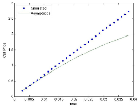
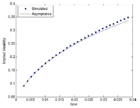
Figure 1: Call (left) and IV (right) with $\sigma=0.3$, $t\in[$1 day; 2 weeks$]$, $H=0.51$

We chose the extreme case $H=0.51$ because, as it turns out, the asymptotics’ accuracy increase as $H$ increases. We see from the above that the IV asymptotics are accurate at a roughly $5\%$-error level for more than 10 days, and remains fairly accurate up to 2 weeks, while the call asymptotics are only accurate at a $5\%$-error level for 2 days, and deteriorate significantly thereafter. Other values of $H$ show similar pictures. The choice to use IV over call prices for calibration purposes in small time is clear. This can of course be verified rigorously on our formulas since our coefficients can be computed numerically as well; this is omitted from our study. The four pictures in Figure 2 show the extremely sharp fit of IV asymptotics over two weeks as $H$ increases, as we mentioned.

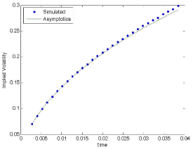
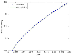
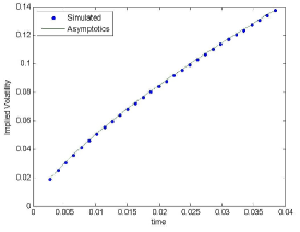
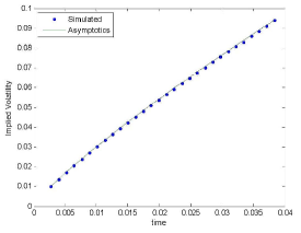
Figure 2: IV with $\sigma=0.3$, $t\in[$1 day; 2 weeks$]$, $H=0.55,0.60$ (top left and right), $H=0.75,0.85$ (bottom left and right).

Since liquidity decreases as time to maturity decreases, it is desirable to use the largest possible time $t_{0}$ such that the relative error in IV approximation does not exceed a given error level, say $1\%$ which would be a high level of accuracy. The table below give an idea of what this means in practice, by computing $t_{0}$ for a $1\%$ level in the above realistic cases: with

$$t_{0}=\max\left\{t:\frac{\text{simulated IV }\left(t\right)-\text{asymptotic IV }\left(t\right)}{\text{simulated IV }\left(t\right)}<0.01\right\}$$

we find :

t0 in days2.34.610.41414.fragments fragmentst0 in days2.34.610.41414\begin{tabular}[]{|l|l|l|l|l|l|}\hline\cr$H$&$0.51$&$0.55$&$0.60$&$0.75$&$0.85$\\ \hline\cr$t_{0}$ in days&$2.3$&$4.6$&$10.4$&$14$&$14$\\ \hline\cr\end{tabular}.

H0.510.550.600.750.85H0.510.550.600.750.85

These values of $t_{0}$ could be considered as rather conservative, due to the choice of $1\%$ accuracy; practitioners may decide to choose a slightly more liberal level. This is evident from the last tables below, in which we show the result of the calibration of $H$ from exact (simulated) option prices, via Theorem 11.

$$T =$$ 1 day

$$H$$ used in simulation

calibrated from IV via Theorem 11

$$T =$$ 2 days

$$H$$ used in simulation

calibrated from IV via Theorem 11

$$T =$$ 7 days

$$H$$ used in simulation

calibrated from IV via Theorem 11

$$T =$$ 14 days

$$H$$ used in simulation

calibrated from IV via Theorem 11

In all cases, even with a 14-day time to maturity, the error in $H$-calibration is no greater than one hundredth (less than $2\%$ relative error). The only difficulty we experience appears to be in differentiating between a model with Brownian scaling ($H=0.50$, no memory in the volatility) and a model with $H>0.50$, except for the very short times to maturity $t=1,2$ days. If liquidity at those levels is adequate, as it may be in heavily traded bond markets, then our calibration can be used with such short horizons. Otherwise a maturity of one week is preferable, particularly for self-similarity indices which are not too close to $0.50$. A maturity of two weeks will work in all cases for scenarios where one is satisfied with a possible error of one hundredth on $H$ calibration; this could be a realistic accuracy level for many users of stochastic volatiltiy models who are currently not using any self-similarity or long-memory assumptions.

References

• [1] M. Abramovitz and I. A. Stegun (Eds.), Handbook of Mathematical Functions, Applied Mathematics Series 55, National Bureau of Standards, Washngton, 1972.
• [2] A. Alexanderian, A brief note on the Karhunen-Loève expansion, technical note, available on users.ices.utexas.edu/$\sim$alen/articles/KL.pdf
• [3] E. Alòs, J. Léon, and J. Vives, On the short-time behavior of the implied volatility for jump-diffusion models with stochastic volatility, Finance Stoch. 11 (2007), 571-589.
• [4] J. Armstrong, M. Forde, M. Lorig, and H. Zhang, Small-time asymptotics under local-stochastic volatility with a jump-to-default: curvature and the heat kernel expansion, available at arXiv:1312.2281, 2013.
• [5] X. Bardina, Kh. Es-Sebaiy, An extension of bifractional Brownian motion, Communications on Stochastic Analysis 5 (2) (2011) 333-340.
• [6] C. Bayer, P. Friz, and J. Gatheral, Pricing under rough volatility, available at http://ssrn.com/abstract=2554754, 2015.
• [7] H. Berestycki, J. Busca, and I. Florent, Computing the implied volatility in stochastic volatility models, Comm. Pure App. Math. 57 (2004), 1352-1373.
• [8] T. Bojdecki, L. G. Gorostiza, and A. Talarczyk, Some extensions of fractional Brownian motion and sub-fractional Brownian motion related to particle systems, Elect. Comm. in Probab., 12 (2007), 161-172.
• [9] F. Caravenna and J. Corbetta, General smile asymptotics with bounded maturity, available at arXiv:1411.1624v1, 2014.
• [10] A. Chronopoulou and F. Viens, Stochastic volatility models with long-memory in discrete and continuous time, Quantitative Finance, 12 (2012), 635-649.
• [11] F. Comte and E. Renault, Long memory in continuous-time stochastic volatility models, Mathematical Finance, 8 (1998), 291-323.
• [12] F. Comte, L. Coutin, and E. Renault, Affine fractional stochastic volatility models, Ann. Finance 8 (2012), 337-378.
• [13] S. Corlay, Quelques aspects de la quantification optimale, et applications en finance (in English, with French summary), Ph.D. Thesis, Université Pierre et Marie Curie, 2011.
• [14] S. Corlay, The Nyström method for functional quantization with an application to the fractional Brownian motion, 2010, hal-00515488, version 1.
• [15] S. Corlay, Properties of the Ornstein-Uhlenbeck bridge, available at https://hal.archives-ouvertes.fr/hal-00875342v4, 2014.
• [16] S. Corlay and G. Pagès, Functional quantization-based stratified sampling methods, avaliable on https://hal.archives-ouvertes.fr/hal-00464088v3, 2014.
• [17] A. Daniluk and R. Muchorski, The approximation of bonds and swaptions prices in a Black-Karasinski model based on the Karhunen-Loève expansion. In: 6th General AMaMeF and Banach Center Conference, 2013.
• [18] P. Deheuvels and G. Martynov, A Karhunen-Loève decomposition of a Gaussian process generated by independent pairs of exponential random variables, J. Funct. Anal., 255 (2008), 23263-2394.
• [19] J.-D. Deuschel, P. K. Friz, A. Jacquier and S. Violante. Marginal density expansions for diffusions and stochastic volatility I: Theoretical foundations. Communications on Pure and Applied Mathematics 67 (2014), 40-82.
• [20] J.-D. Deuschel, P. K. Friz, A. Jacquier and S. Violante. Marginal density expansions for diffusions and stochastic volatility I: Applications. Communications on Pure and Applied Mathematics 67 (2014), 321-350.
• [21] P. Embrechts and M. Maejima, Selfsimilar Processes, Princeton University Press 2002.
• [22] J. Feng, M. Forde, and J.-P. Fouque, Short-maturity asymptotics for a fast mean-reverting Heston stochastic volatility model, SIAM J. Financial Math. 1 (2010), 126-141.
• [23] J. Feng, J.P. Fouque, and R. Kumar, Small-time asymptotics for fast mean-reverting stochastic volatility models, Ann. Appl. Probab. 22 (2012), 1541-1575.
• [24] J. E. Figueroa-López and Ch. Houdré, Small-time expansions for the transition distributions of Lévy processes, Stochastic Process. Appl. 119 (2009), 3862-3889.
• [25] J. E. Figueroa-López and M. Forde, The small-maturity smile for exponential Lévy models, SIAM J. Financial Math. 3 (2012), 33-65.
• [26] M. Forde and A. Jacquier, Small-time asymptotics for implied volatility under the Heston model, IJTAF, 12 (2009), 861-876.
• [27] M. Forde and A. Jacquier. Small-time asymptotics for an uncorrelated local-stochastic volatility model, Applied Mathematical Finance, 18 (2011), 517-535.
• [28] M. Forde and A. Jacquier, Small-time asymptotics for implied volatility under a general local-stochastic volatility model, Appl. Math. Finance 18 (2011), 517-535.
• [29] M. Forde, A. Jacquier, and R. Lee, The small-time smile and term structure of implied volatility under the Heston model, SIAM J. Finan. Math. 3 (2012), 690–708.
• [30] M. Forde, A. Jacquier, and A. Mijatović, Asymptotic formulae for implied volatility in the Heston model, Proc. R. Soc. A 466 (2010), 3593-3620.
• [31] M. Forde and H. Zhang, Asymptotics for rough stochastic volatility and Lévy models, 2015.
• [32] J.-P. Fouque, G. Papanicolaou, K. R. Sircar, Derivatives in Financial Markets with Stochastic Volatility, Cambridge U.P., 2000.
• [33] M. Fukasawa, Asymptotic analysis for stochastic volatility: martingale expansion, Finance Stoch. 15 (2011), 635-654.
• [34] M. Fukasawa, Short-time at-the-money skew and fractional rough volatility, available at arXiv:1501.06980v1, 2015.
• [35] K. Gao and R. Lee, Asymptotics of implied volatility to arbitrary order, to appear in Finance and Stochastics, 2015. Available at http://papers.ssrn.com/sol3/papers.cfm?abstract_id=1768383.
• [36] J. Gatheral (joint work with C. Bayer, P. Friz, T. Jaisson, A. Lesniewski, and M. Rosenbaum), Rough volatility, slides, National School of Development, Peking University, Tuesday November 4, 2014.
• [37] J. Gatheral (joint work with C. Bayer, P. Friz, T. Jaisson, A. Lesniewski, and M. Rosenbaum), Volatility is Rough, Part 2: Pricing, slides, Workshop on Stochastic and Quantitative Finance, Imperial College London, Saturday November 29, 2014.
• [38] J. Gatheral, T. Jaisson, and M. Rosenbaum, Volatility is rough, available at arXiv:1410.3394, 2014.
• [39] J. Gatheral, E. Hsu, P. Laurence, C. Ouyang, and T-H. Wang, Asymptotics of implied volatility in local volatility models, Mathematical Finance 22 (2012), 591-620.
• [40] H. Guennon, A. Jacquier, and P. Roome, Asymptotic behavior of the fractional Heston model, available at arXiv:1411.7653, 2014.
• [41] A. Gulisashvili. Analytically Tractable Stochastic Stock Price Models, Springer-Verlag Berlin Heidelberg 2012.
• [42] A. Gulisashvili, B. Horvath, and A. Jacquier, Mass at zero and small-strike implied volatility expansion in the SABR model, submitted for publication, available at arXiv:1502.03254v1, 2015, and at http://ssrn.com/abstract=2563510, 2015.
• [43] A. Gulisashvili and E. M. Stein, Asymptotic behavior of the stock price distribution density and implied volatility in stochastic volatility models, Applied Mathematics and Optimization 61 (2010), 287-315.
• [44] A. Gulisashvili, F. Viens, and X. Zhang, Extreme-strike asymptotics for general Gaussian stochastic volatility models, available at arXiv:1502.05442v1, 2015.
• [45] P. S. Hagan, D. Kumar, A. Lesniewski, and D. E. Woodward, Managing smile risk, Wilmott Magazine (2003).
• [46] P. S. Hagan, A. Lesniewski, D. Woodward, Probability Distribution in the SABR Model of Stochastic Volatility, in P. K. Friz, J. Gatheral, A. Gulisashvili, A. Jacquier, and J. Teichmann, Editors, Large Deviations and Asymptotic Methods in Finance, Springer International Publishing Switzerland 2015. pp. 1-36.
• [47] P. Henry-Labordère, Analysis, Geometry and Modeling in Finance: Advanced Methods in Option Pricing, Chapman & Hall/CRC, Financial Mathematics Series, 2008.
• [48] C. Houdré and J. Villa, An example of infinite-dimensional quasi-helix, Contemp. Math., Am. Math. Soc 336 (2003), 195-201.
• [49] R. Lee, The moment formula for implied volatility at extreme strikes, Math. Finance 14 (2004), 469-480.
• [50] S. C. Lim, Fractional Brownian motion and multifractional Brownian motion of Riemann-Liouville type, Journal of Physics A: Mathematical and General 34 (2001), 1301.
• [51] A. Medvedev and O. Scaillet, Approximation and calibration of short-term implied volatilities under jump-diffusion stochastic volatility, Rev. Financial Studies 20 (2007), 427–459.
• [52] R. Vilela Mendez, M. J. Olivejra, and A. M. Rodriguez, The fractional volatility model: No-arbitrage, leverage and completeness, available on arXiv:1205.2866v1, 2012.
• [53] P. Tankov and A. Mijatović, A new look at short-term implied volatility in asset price models with jumps, to appear in Mathematical Finance, available at arXiv:1207.0843, 2012.
• [54] J. Muhle-Karbe and M. Nutz, Small-time asymptotics of option prices and first absolute moments, Journal of Applied Probability, 48 (2011), 1003-1020.
• [55] I. Nourdin, Selected Aspects of Fractional Brownian Motion, Springer Verlag Italia 2012.
• [56] D. Nualart, Fractional Brownian motion: stochastic calculus and applications, Proceedings of the International Congress of Mathematicians, Madrid, Spain, European Mathematical Society, 2006, pp. 1541-1562.
• [57] L. Paulot, Asymptotic implied volatility at the second order with application to the SABR model, in P. K. Friz, J. Gatheral, A. Gulisashvili, A. Jacquier, and J. Teichmann, Editors, Large Deviations and Asymptotic Methods in Finance, Springer International Publishing Switzerland 2015.
• [58] E. Renault and N. Touzi, Option Hedging and Implicit Volatilities, Mathematical Finance 6 (1996), 279-302.
• [59] M. Roper and M. Rutkowski, On the relationship between the call price surface and the implied volatility surface close to expiry, International Journal of Theoretical and Applied Finance, 12(2009), 427-441.
• [60] M. Rosenbaum, Estimation of the volatility persistence in a discretely observed diffusion model, Stochastic Processes and their Applications 118 (2008), 1434-1462.
• [61] S. Rostek, Option Pricing in Fractional Brownian Markets, Springer-Verlag Berlin Heidelberg 2009.
• [62] E. Stein and J. Stein, Stock price distributions with stochastic volatility: an analytic approach, Rev. Financ. Stud. 4 (1991), 727-752.
• [63] S. Torres, C. A. Tudor, F. G. Viens, Quadratic variations for the fractional-colored stochastic heat equation, Electron. J. Probab. 19 (2014), 1-51.
• [64] C. A. Tudor, Analysis of Variations for Self-similar Processes, Springer International Publishing Switzerland 2013.
• [65] A. M. Yaglom, Correlation Theory of Stationary and Related Random Functions, Vol. I, Springer-Verlag New York 1987.