SPARSE AND ROBUST LINEAR REGRESSION:

AN OPTIMIZATION ALGORITHM AND

ITS STATISTICAL PROPERTIES

Shota Katayama and Hironori Fujisawa

Tokyo Institute of Technology and The Institute of Statistical Mathematics

Abstract: This paper studies sparse linear regression analysis with outliers in the responses. A parameter vector for modeling outliers is added to the standard linear regression model and then the sparse estimation problem for both coefficients and outliers is considered. The $\ell_{1}$ penalty is imposed for the coefficients, while various penalties including redescending type penalties are for the outliers. To solve the sparse estimation problem, we introduce an optimization algorithm. Under some conditions, we show the algorithmic and statistical convergence property for the coefficients obtained by the algorithm. Moreover, it is shown that the algorithm can recover the true support of the coefficients with probability going to one.

Key words and phrases: Sparse linear regression, robust estimation, algorithmic and statistical convergence, support recovery.

1. Introduction

Linear regression with a large number of covariates is a general and fundamental problem in recent data analysis. A standard method to overcome this problem is the least absolute shrinkage and selection operator (Lasso) proposed by Tibshirani (1996). For a large number of covariates, it is natural to assume the sparsity which means that many of the covariates are not relevant to the responses. The Lasso can draw relevant covariates automatically and simultaneously estimate the remaining coefficients to be zero. From the theoretical point of view, the Lasso has been largely studied. For instance, Bickel et al. (2009), Meinshausen and Yu (2009) and Wainwright (2009) gave the convergence rate under several norms and showed that the Lasso estimates can recover the true support of the coefficients. See also Efron et al. (2004), Zhao and Yu (2006), Zou (2006) and van de Geer and Bühlmann (2009).

Recent linear regression analysis requires some complex structures in addition to a large number of covariates. One of them is an outlier structure. This structure often appears in many applications such as signal detection, image and speech processing, communication network and so on. It is well known that the standard method which uses the $\ell_{2}$ loss outputs inaccurate estimates when outliers exist. The most popular way for robustifying against the outliers is to use the M-estimation procedure which replaces the $\ell_{2}$ loss by an other loss with a bounded influence function; e.g., the Huber’s, the skipped-mean and the Hampel’s robust loss (see, for instance, Huber and Ranchetti (2009) for more details). However, optimizing such a robust loss function with a sparse penalty requires much computational cost. The $\ell_{2}$ loss function is easier to deal with. Recently, She and Owen (2011) proposed a novel approach for robust parameter estimation, using an outlier model where a parameter vector for modeling outliers is added to the standard linear regression model. The corresponding $\ell_{2}$ loss function with a sparse penalty for the outlier parameter vector is optimized. The connection between sparse penalties and robust loss functions was also illustrated.

This paper studies sparse and robust linear regression based on their outlier model from a theoretical point of view, which was not treated in She and Owen (2011). Some theoretical analyses were discussed by Nguyen and Tran (2013), but only the $\ell_{1}$ penalty was used for the outlier parameters. Their results were derived from the fact that the resulting estimate is a global optimum. As She and Owen (2011) showed, many penalties having good robustness are non-convex and then the resulting estimate is often a local optimum. A general theory including non-convex penalties is thus of great interest.

Main contributions in this paper are the following. We consider a larger class of penalties for outlier parameters including non-convex penalties and then derive some statistical properties. To avoid the problem of local optima, we directly analyze estimated coefficients which an optimization algorithm outputs. We provide the upper bound of its $\ell_{2}$ error, which is divided by an algorithmic error and a statistical error. It is also shown that the algorithm can recover the true support of the coefficients. Thus, this paper bridges a gap between the statistical theory and the computation algorithm, which arises in using non-convex penalties.

The remainder of this paper is organized as follows. We introduce the model and the optimization algorithm in Section 2. In Section 3, theoretical analyses for the estimated coefficients which the algorithm outputs are provided. We report numerical performances in Section 4. All the proofs are in Section 5.

Throughout the paper, a bold symbol denotes a matrix or a vector and its element is written by the fine symbol, e.g., $\bm{A}=(a_{ij})$ for $\bm{A}\in\mathbb{R}^{m\times n}$ and $\bm{a}=(a_{1},\dots,a_{m})^{T}$ for $\bm{a}\in\mathbb{R}^{m}$. For any vector $\bm{a}\in\mathbb{R}^{m}$ and $1\leq q<\infty$, we define the $\ell_{q}$ norms as $\|\bm{a}\|_{q}=(\sum_{i=1}^{m}|a_{i}|^{q})^{1/q}$ and define the $\ell_{0}$ and $\ell_{\infty}$ norms as $\|\bm{a}\|_{0}=|\{i|\,a_{i}\neq 0\}|$ and $\|\bm{a}\|_{\infty}=\max_{1\leq i\leq m}|a_{i}|$, respectively. Given a set $S\subset\{1,\dots,m\}$, $\bm{a}_{S}$ denotes the sub-vector having the elements of $\bm{a}$ corresponding to the set $S$, that is, $\bm{a}_{S}=\{a_{i}|\;i\in S\}$. For any two vectors $\bm{a},\bm{b}\in\mathbb{R}^{m}$, $\langle\bm{a},\bm{b}\rangle$ denotes the standard inner product. We define the matrix $\ell_{1}$ norm as $\|\bm{A}\|_{\ell_{1}}=\max_{1\leq j\leq n}\sum_{i=1}^{m}|a_{ij}|$ and for any symmetric matrix $\bm{B}\in\mathbb{R}^{m\times m}$, we define its largest eigenvalue as $\xi_{max}(\bm{B})$. For two positive sequences $a_{n},b_{n}$ depending on $n$, the notation $a_{n}=O(b_{n})$ means that there exists a finite constant $C>0$ such that $a_{n}\leq Cb_{n}$ for a sufficiently large $n$, while $a_{n}=\Omega(b_{n})$ means that $a_{n}\geq Cb_{n}$. Also, the notation $a_{n}=o(b_{n})$ means that $a_{n}/b_{n}\to 0$ as $n$ goes to infinity.

2. Sparse and robust linear regression

2.1. Model and parameter estimation

Consider the linear regression model with outliers

$$\bm{y}=\bm{X}\bm{\beta^{*}}+\sqrt{n}\bm{\gamma^{*}}+\bm{\varepsilon},$$ (2.1)

where $\bm{y}=(y_{1},\dots,y_{n})^{T}$ is an $n$ dimensional response vector, $\bm{X}=(x_{ij})=(\bm{x}_{1},\dots,\bm{x}_{n})^{T}$ is an $n\times p$ covariate matrix, $\bm{\beta}^{*}$ is a $p$ dimensional unknown coefficient vector, $\bm{\gamma}^{*}$ is an $n$ dimensional unknown vector whose nonzero elements correspond to outliers and $\bm{\varepsilon}$ is an $n$ dimensional random error vector. In the model (2.1), we assume that the $\ell_{2}$ norm of columns of $\bm{X}$ is $\sqrt{n}$. Correspondingly, the coefficient of $\bm{\gamma}^{*}$ is assumed to be $\sqrt{n}$ to match its scale with the columns of $\bm{X}$. The model (2.1) can be found also in She and Owen (2011) and Nguyen and Tran (2013). Our purpose is to estimate $\bm{\beta}^{*}$ accurately even when the number of covariates is large. In this case, it is natural to assume that $\bm{\beta}^{*}$ has many zero elements (sparse). Moreover, we can assume that $\bm{\gamma}^{*}$ is also sparse since the number of outliers is usually not large. For this sparse structure, we introduce sparse penalties for both coefficients and outliers. The parameters are estimated by solving the optimization problem

$$\mathop{\rm argmin}\limits_{\bm{\beta}\in\mathbb{R}^{p},\bm{\gamma}\in\mathbb{R}^{n}}\frac{1}{2n}\|\bm{y}-\bm{X}\bm{\beta}-\sqrt{n}\bm{\gamma}\|_{2}+\lambda_{\beta}\sum_{j=1}^{p}w_{\beta,j}|\beta_{j}|+\lambda_{\gamma}\sum_{i=1}^{n}w_{\gamma,i}P(\gamma_{i}),$$ (2.2)

where $\lambda_{\beta}>0$ and $\lambda_{\gamma}>0$ are tuning parameters for $\bm{\beta}$ and $\bm{\gamma}$, respectively and $P(\cdot)$ is a penalty function that encourages sparsity. We often use a redescending type of $P(\cdot)$, since it can yield a small bias against strong outliers. We consider the adaptive Lasso (Zou (2006)) type optimization problem. In (2.2), $w_{\beta,i}$ and $w_{\gamma,j}$ are known weights. Suppose that we have the preliminary estimators $\tilde{\bm{\beta}}=(\tilde{\beta}_{1},\dots,\tilde{\beta}_{p})^{T}$ and $\tilde{\bm{\gamma}}=(\tilde{\gamma}_{1},\dots,\tilde{\gamma}_{n})^{T}$. The weights are typically defined as $w_{\beta,j}=1/|\tilde{\beta_{j}}|$ and $w_{\gamma,i}=1/|\tilde{\gamma}_{i}|$. For the details of the preliminary estimators used in this paper, see Section 3.3.

2.2. Optimization algorithm

Algorithm 1

  Step 1. Initialize $k\leftarrow 0$, $\bm{\beta}^{k}\leftarrow\bm{\beta}^{init}$ and $\bm{\gamma}^{k}\leftarrow{\rm argmin}_{\bm{\gamma}}L(\bm{\beta}^{0},\bm{\gamma})$.

  Step 2. Update $k\leftarrow k+1$,

$$\bm{\beta}^{k} \leftarrow{\rm argmin}_{\bm{\beta}}L(\bm{\beta},\bm{\gamma}^{k-1}),$$ (2.3)

$$\bm{\gamma}^{k} \leftarrow{\rm argmin}_{\bm{\gamma}}L(\bm{\beta}^{k},\bm{\gamma}).$$ (2.4)

  Step 3. If they converge, then output current $(\bm{\beta}^{k},\bm{\gamma}^{k})$ and stop the algorithm, otherwise return to Step 2.

Let $L(\bm{\beta},\bm{w})$ be the objective function in (2.2). To solve the optimization problem (2.2), we introduce Algorithm 1. This algorithm surely converges since it satisfies that

$$L(\bm{\beta}^{0},\bm{\gamma}^{0})\geq L(\bm{\beta}^{1},\bm{\gamma}^{0})\geq L(\bm{\beta}^{1},\bm{\gamma}^{1})\geq\cdots\geq 0$$

from its construction. We also note that the optimization problem in (2.3) can be solved by a typical way such as the coordinate descent algorithm (Friedman et al. (2010)). The optimization problem in (2.4) can be rewritten as

$$\mathop{\rm argmin}\limits_{\bm{\gamma}\in\mathbb{R}^{n}}\frac{1}{2n}\sum_{i=1}^{n}\big{\{}(y_{i}-\bm{x}_{i}^{T}\bm{\beta}^{k}-\sqrt{n}\gamma_{i})^{2}+\lambda_{\gamma}w_{\gamma,i}P(\gamma_{i})\big{\}}.$$

Suppose that the problem ${\rm argmin}_{x}(z-x)^{2}/2+\lambda P(x)$ has the explicit solution $\Theta(z;\lambda)$. Then, (2.4) can be written as

$$\gamma_{i}^{k}\leftarrow\frac{1}{\sqrt{n}}\Theta(y_{i}-\bm{x}_{i}^{T}\bm{\beta}^{k};\lambda_{\gamma}w_{\gamma,i}),\quad i=1,\dots,n,$$

where $\gamma_{i}^{k}$ is the $i$th element of $\bm{\gamma}^{k}$. Let this expression be denoted by $\bm{\gamma}^{k}\leftarrow h(\bm{\beta}^{k})$. Then, the step 2 can be expressed with only the update of $\bm{\beta}$ as

$$\bm{\beta}^{k}\leftarrow\mathop{\rm argmin}\limits_{\bm{\beta}\in\mathbb{R}^{p}}L\big{\{}\bm{\beta},h(\bm{\beta}^{k-1})\big{\}}.$$

The function $\Theta(z;\lambda)$ is often called as the thresholding function. As seen in Antoniadis and Fan (2001), many sparse penalties, including the $\ell_{1}$, $\ell_{0}$ and smoothly clipped absolute deviation (SCAD; Fan (1997)) penalties, have an explicit solution $\Theta(z;\lambda)$. The $\ell_{1}$ penalty leads to the soft thresholding function $\Theta(z;\lambda)={\rm sgn}(z)\max(|z|-\lambda,0)$ where ${\rm sgn}(\cdot)$ denotes the sign function, and the $\ell_{0}$ penalty leads to the hard thresholding function $\Theta(z;\lambda)=zI(|z|>\lambda)$, where $I(A)$ denotes the indicator function on the event $A$. For the SCAD penalty, the corresponding thresholding function is given by

$$\Theta(z;\lambda)=\begin{cases}{\rm sgn}(z)(|z|-\lambda)&{\rm if\ }|z|\leq 2\lambda\\ \frac{(a-1)z-a\lambda{\rm sgn}(z)}{a-2}&{\rm if\ }2\lambda<|z|\leq a\lambda\\ z&{\rm if\ }|z|>a\lambda,\end{cases}$$

where $a=3.7$ is recommended by Fan and Li (2001).

2.3. Connection to robust $M$-estimators

Similarly in She and Owen (2011), our procedure also has a close connection to robust $M$-estimators.

Proposition 1.

Let $\hat{\bm{\beta}}$ be the coefficient output of Algorithm 1 and let $\psi(z;\lambda)=z-\Theta(z;\lambda)$, where $\Theta(\cdot;\lambda)$ is a thresholding function yielded from a penalty function $P(\cdot)$. Then, for $j=1,\dots,p$, it follows that

$$\frac{1}{n}\sum_{i=1}^{n}x_{ij}\psi(y_{i}-\bm{x}_{i}^{T}\hat{\bm{\beta}};\lambda_{\gamma}w_{\gamma,i})+\lambda_{\beta}w_{\beta,j}\partial|\hat{\beta}_{j}|=0,$$ (2.5)

where $\partial|\hat{\beta}_{j}|$ is the subgradient of $|\hat{\beta}_{j}|$ which means that $\partial|\hat{\beta}_{j}|={\rm sgn}(\hat{\beta}_{j})$ if $\hat{\beta}_{j}\neq 0$, $\partial|\hat{\beta}_{j}|\in[-1,1]$ otherwise.

Proposition 1 shows that the output $\hat{\bm{\beta}}$ satisfies the estimating equations (2.5) with the $\psi$ function and the $\ell_{1}$ penalty. Thus, our algorithm is closely related to the optimization problem

$$\mathop{\rm argmin}\limits_{\bm{\beta}\in\mathbb{R}^{p}}\frac{1}{2n}\sum_{i=1}^{n}\Psi(y_{i}-\bm{x}_{i}^{T}\bm{\beta};\lambda_{\gamma}w_{\gamma,i})+\lambda_{\beta}\sum_{j=1}^{p}w_{\beta,j}|\beta_{j}|,$$ (2.6)

where $\frac{d}{dt}\Psi(t;\lambda)=\psi(t;\lambda)$. It may take much computational cost to directly solve (2.6), particularly when the function $\Psi(\cdot;\lambda)$ is non-convex. For the fast computation, we can use the first-order approximation of $\Psi(\cdot;\lambda)$, but it loses the information of the original function. For this reason, we use Algorithm 1 instead of solving (2.6).

The relationship between sparse penalties and robust loss functions are stated through the equation $\psi(z;\lambda)=z-\Theta(z;\lambda)$. For instance, the $\ell_{1}$ penalty corresponds to the Huber’s loss, the $\ell_{0}$ penalty to the skipped-mean loss and the SCAD penalty to the Hampel’s loss. She and Owen (2011) gave their illustrations and more details. One measure to characterize the robust loss function is the redescending property. It means that $\psi(z;\lambda)$ goes to $0$, equivalently $|z-\Theta(z;\lambda)|$ goes to $0$, as $|z|$ goes infinity. The soft thresholding function which corresponds to the $\ell_{1}$ penalty does not have the redescending property, but the hard and SCAD thresholding functions which correspond to the non-convex penalties have it. Some other non-convex penalties including the non-negative garrote penalty (Garrote; Gao (1998)) and the minimax concave penalty (MCP; Zhang (2010)) also lead to that property. Thus, penalties yielding good robustness are non-convex.

3. Theoretical Analysis

The optimization problem (2.2) with a non-convex penalty $P(\cdot)$ suffers from local minima. We may be able to give a theoretical analysis for a global minimum of (2.2), but it is unclear which optimization algorithm can actually output the global minimum. To avoid such a problem, we directly analyze the output of Algorithm 1. Some theoretical analyses for computable solutions in linear regression model without outliers were provided by Zhang and Zhang (2012), Fan and Lv (2013) and Fan and Lv (2014), but our analysis is essentially different from theirs. They first derived some properties for a global minimum and then showed that a computable solution shared those properties under additional conditions for the solution.

3.1. Notations

First, we prepare some notations. Let $S^{*}={\rm supp}(\bm{\beta}^{*})=\{i|\,\beta_{i}^{*}\neq 0\}\subset\{1,\dots,p\}$ and $G^{*}={\rm supp}(\bm{\gamma}^{*})\subset\{1,\dots,n\}$. These support sizes are written by $s^{*}=|S^{*}|$ and $g^{*}=|G^{*}|$. For the preliminary estimators, similarly let $\tilde{S}={\rm supp}(\tilde{\bm{\beta}})$ and $\tilde{G}={\rm supp}(\tilde{\bm{\gamma}})$ with sizes $\tilde{s}=|\tilde{S}|$ and $\tilde{g}=|\tilde{G}|$. We define the restricted smallest eigenvalue $\delta_{min}$ as

$$\delta_{min}(u)=\inf_{\|\bm{\delta}\|_{0}\leq u}\frac{\|\bm{X}\bm{\delta}\|_{2}^{2}}{n\|\bm{\delta}\|_{2}^{2}}$$ (3.1)

and the (doubly) restricted largest eigenvalue $\delta_{max}$ as

$$\delta_{max}(u,u^{\prime})=\sup_{\|\bm{\delta}\|_{0}\leq u}\sup_{|G|\leq u^{\prime}}\frac{\|\bm{X}_{(G)}\bm{\delta}\|_{2}^{2}}{n\|\bm{\delta}\|_{2}^{2}}$$ (3.2)

where $\bm{X}_{(G)}$ is the sub-matrix having the rows of $\bm{X}$ corresponding to the set $G$, that is, $\bm{X}_{(G)}=\{x_{ij}|\;i\in G,1\leq j\leq p\}$. The restricted eigenvalue is popular in the analysis of the Lasso (see, e.g., Bickel et al. (2009)), but our $\delta_{max}$ is slightly different from the existing one. The restriction is imposed on rows of $\bm{X}$ in addition to columns, corresponding to the outliers. We shall provide an asymptotic analysis as $n$ goes to infinity. In our theory, $p$, $s^{*}$ and $g^{*}$ may go to infinity depending on $n$. Notice that the restricted eigenvalues also depend on $n$.

3.2. Properties of Algorithm 1 output

To derive a convergence property of Algorithm 1, we require the following conditions for the random error vector $\bm{\varepsilon}=(\varepsilon_{1},\dots,\varepsilon_{n})^{T}$, the thresholding function $\Theta(\cdot;\lambda)$ and the preliminary estimator $(\tilde{\bm{\beta}},\tilde{\bm{\gamma}})$.

Condition 1.

The errors $\varepsilon_{1},\dots,\varepsilon_{n}$ are independently and identically distributed as the zero mean sub-Gaussian distribution with a parameter $\sigma>0$, that is, $\mathbb{E}(\varepsilon_{i})=0$ and $\mathbb{E}\{\exp(t\varepsilon_{i})\}\leq\exp(t^{2}\sigma^{2}/2)$ for all $t\in\mathbb{R}$.

Condition 2.

The thresholding function $\Theta(\cdot;\lambda)$ satisfies that $\Theta(x;\lambda)=0$ if $|x|\leq\lambda$ and $|\Theta(x;\lambda)-x|\leq\lambda$ for all $x\in\mathbb{R}$.

Condition 3.

There exist a sequence $a_{n,1}\to 0$ and a constant $\kappa>0$ such that $\|\tilde{\bm{\beta}}-\bm{\beta}^{*}\|_{2}+\|\tilde{\bm{\gamma}}-\bm{\gamma}^{*}\|_{2}\leq\tilde{C}a_{n,1}$ and $\delta_{min}(\tilde{s})\geq\kappa$ with probability going to one, where $\tilde{C}$ is some positive constant.

Condition 1 assumes that the errors in the model (2.1) belong to the sub-Gaussian distribution family. As seen in Vershynin (2012), this family covers the Gaussian, Bernoulli and any distributions with a bounded support. Condition 2 decides a class of thresholding functions (or equivalently penalties) which can be handled by our theory. For instance, this class includes the soft, hard, non-negative garrote, SCAD and MCP thresholding functions. The first half claim in Condition 3 implies consistent preliminary estimators at the rate $a_{n,1}$. Under this condition, we have $|\tilde{\beta}_{j}|\geq|\beta_{j}^{*}|-|\tilde{\beta}_{j}-\beta_{j}^{*}|\geq|\beta_{j}^{*}|-\tilde{C}a_{n,1}$ for $j\in S^{*}$ by the triangle inequality. Hence, if $\min_{j\in S^{*}}|\beta_{j}^{*}|>\tilde{C}a_{n,1}$, then $|\tilde{\beta}_{j}|>0$ for $j\in S^{*}$. Similarly, we can show that if $\min_{i\in G^{*}}|\gamma_{i}^{*}|>\tilde{C}a_{n,1}$ then $|\tilde{\gamma}_{i}|>0$ for $i\in G^{*}$. Thus, Condition 3 leads to the screening property that $S^{*}\subset\tilde{S}$ and $G^{*}\subset\tilde{G}$ if

$$\min\big{\{}\min_{j\in S^{*}}|\beta_{j}^{*}|,\min_{i\in G^{*}}|\gamma_{i}^{*}|\big{\}}>\tilde{C}a_{n,1}.$$ (3.3)

The second half claim in Condition 3 is well known as the sparse Riesz condition (Zhang and Huang (2008)) if $\tilde{s}$ is non-random. When we use a preliminary estimator which has a non-random upper bound $s_{u}$, it reduces to $\delta_{min}(s_{u})\geq\kappa$. In Section 3.3, we shall clarify the order of $a_{n,1}$ and the non-random upper bound of $\tilde{s}$ for some preliminary estimators. For a technical reason, we re-define the weights $w_{\beta,j}$ and $w_{\gamma,i}$ using a constant $R_{w}>0$ by

$$w_{\beta,j}=\max\bigg{(}\frac{1}{|\tilde{\beta}_{j}|},\frac{1}{R_{w}}\bigg{)},\quad w_{\gamma,i}=\min\bigg{(}\frac{1}{|\tilde{\gamma}_{i}|},R_{w}\bigg{)}$$ (3.4)

for $i\in\tilde{G}$ and $j\in\tilde{S}$. From these restrictions, it follows that $\min_{j\in\tilde{S}}w_{\beta,j}\geq R_{w}^{-1}$ and $\max_{i\in\tilde{G}}w_{\gamma,i}\leq R_{w}$. They are required to exclude the case where $w_{\beta,j}\to 0$ and $w_{\gamma,i}\to\infty$ as $n$ goes to infinity in our theory. Although these are the same as the originals if $R_{w}$ is large, it is convenient for deriving the following theories. Moreover, the same result holds if different constants $R_{w,\beta}$ and $R_{w,\gamma}$ are used in (3.4).

Under these conditions, we can show the algorithmic and statistical convergence property of Algorithm 1.

Theorem 1.

Assume Conditions 1–3 and (3.3). Let

$$\lambda_{\beta}\geq 2CR_{w}\sqrt{\frac{\sigma^{2}\log p}{n}},\quad\lambda_{\gamma}\leq\frac{Cn}{R_{w}\max_{j\in\tilde{S}}\sum_{i\in\tilde{G}}|x_{ij}|}\sqrt{\frac{\sigma^{2}\log p}{n}}$$

for a constant $C>\sqrt{2}$ and $R_{w}>0$ used in (3.4). Then, for any iteration $k\geq 1$ and any initial value $\bm{\beta}^{init}$ in Algorithm 1,

$$\|\bm{\beta}^{k}-\bm{\beta}^{*}\|_{2}\leq\rho^{k}\|\bm{\beta}^{init}-\bm{\beta}^{*}\|_{2}+2\kappa^{-1}\sqrt{s^{*}}\lambda_{\beta}\big{(}R_{w}^{-1}+\max_{j\in S^{*}}w_{\beta,j}\big{)}\sum_{i=0}^{k-1}\rho^{i},$$ (3.5)

with probability going to one, where $\rho=2\kappa^{-1}\delta_{max}(\tilde{s},\tilde{g})$.

The first term of the right hand side of (3.5) can be regarded as the algorithmic error. It represents the effect of an initial value $\bm{\beta}^{init}$ in Algorithm 1. This shows that if $\rho<1$ then the effect vanishes from the bound exponentially as the number of iterations increases. Since $|\xi_{max}(\bm{M})|\leq\|\bm{M}\|_{\ell_{1}}$ for any symmetric matrix $\bm{M}$, we have

$$\delta_{max}(\tilde{s},\tilde{g})\leq\max_{1\leq i\leq n;1\leq j\leq p}x_{ij}^{2}\frac{\tilde{s}\tilde{g}}{n}.$$ (3.6)

Thus, if $\max_{ij}x_{ij}^{2}a_{n,2}^{2}=o(n)$, we have $\rho<1$ for sufficiently large $n$ with probability going to one, where $a_{n,2}$ shall be defined later in Condition 4. The second term can be regarded as the statistical error. We notice that $\max_{j\in S^{*}}w_{\beta,j}=O(1)$ with probability going to one if $\min_{j\in S^{*}}|\beta_{j}^{*}|=\Omega(1)$. In this case, the second term has $O(\sqrt{s^{*}}\lambda_{\beta})$, which is equivalent to the order of the standard Lasso excluding the term $\sqrt{n}\bm{\gamma}^{*}$ from the model (2.1) in advance.

Theorem 1 shows only the convergence result for the output. Next, we shall show that the output can recover the true support. We need an extra condition and a corollary.

Condition 4.

There exist a constant $C>0$ and a sequence $a_{n,2}$, which may diverge, such that $\max(\tilde{s},\tilde{g})\leq Ca_{n,2}$ with probability going to one.

Corollary 1.

Assume Conditions 1–4, (3.3), $\max_{ij}|x_{ij}|=O(1)$, $\min_{j\in S^{*}}|\beta_{j}^{*}|=\Omega(1)$ and $a_{n,2}^{2}=o(n)$. Let $\lambda_{\beta}\geq C_{\beta}\{(\log p)/n)\}^{1/2}$ and $\lambda_{\gamma}\leq C_{\gamma}\frac{n}{a_{n,2}}\{(\log p)/n\}^{1/2}$ with some constants $C_{\beta}>0$ and $C_{\gamma}>0$. If there exist some $k_{0}\geq 1$ and $C_{0}>0$ such that $\mathbb{P}(\|\bm{\beta}^{init}-\bm{\beta}^{*}\|_{2}\leq C_{0}\rho^{-k_{0}}\sqrt{s^{*}}\lambda_{\beta})\to 1$, then it follows that $\mathbb{P}(\|\bm{\beta}^{k}-\bm{\beta}^{*}\|_{2}\leq C\sqrt{s^{*}}\lambda_{\beta})\to 1$ for any $k\geq k_{0}$ for some constant $C>0$.

When $\max_{i,j}|x_{ij}|=O(1)$ and $a_{n,2}^{2}=o(n)$, we have $\rho=o(1)$. Consequently, Corollary 1 can be immediately obtained from Theorem 1. The requirement $\mathbb{P}(\|\bm{\beta}^{init}-\bm{\beta}^{*}\|_{2}\leq C_{0}\rho^{-k_{0}}\sqrt{s^{*}}\lambda_{\beta})\to 1$ is not so restrictive since $\rho=o(1)$. If we use $\tilde{\bm{\beta}}$ for the initial value $\bm{\beta}^{init}$, then the condition $(a_{n,2}^{2}/n)^{k_{0}}a_{n,1}=O(\sqrt{s^{*}}\lambda_{\beta})$ is required. From Corollary 1, we can show a theorem about the support recovery. It should be noted that we only need to analyze the elements of $\bm{\beta}^{k}$ on $\tilde{S}\cap S^{*^{c}}$ since the screening property $S^{*}\subset\tilde{S}$ holds.

Theorem 2.

Assume the same conditions as in Corollary 1. If $\log p=O(\log n)$, $\sqrt{\log n}=o(\sqrt{n}\min_{i\in G^{*}}|\gamma_{i}^{*}|)$, $a_{n,2}s^{*}=o(n)$ and $a_{n,1}\max\big{(}\sqrt{a_{n,2}s^{*}},g^{*}/\sqrt{n}\big{)}=o(1)$, then we have $\mathbb{P}\big{(}\bm{\beta}^{k}_{\tilde{S}\cap S^{*^{c}}}=\bm{0}\big{)}\to 1$ for any $k\geq k_{0}+1$, where $k_{0}$ is defined in Corollary 1.

3.3. Preliminary estimator and its properties

In the previous section, some statistical properties are derived for general preliminary estimators. In this section, we introduce a concrete example and specify the orders $a_{n,1}$ and $a_{n,2}$ in Conditions 3 and 4. Let us consider the Lasso type preliminary estimators of $\tilde{\bm{\theta}}=(\tilde{\bm{\beta}}^{T},\tilde{\bm{\gamma}}^{T})^{T}$, given by

$$\tilde{\bm{\theta}}=\mathop{\rm argmin}\limits_{\bm{\theta}\in\mathbb{R}^{np}}\frac{1}{2n}\|\bm{y}-\bm{Z}\bm{\theta}\|_{2}^{2}+\lambda_{\theta}\|\bm{\theta}\|_{1},$$ (3.7)

where $\lambda_{\theta}>0$ is the tuning parameter and $\bm{Z}=(\bm{X},\sqrt{n}\bm{I}_{n})$. The estimator $\tilde{\bm{\theta}}$ is a simple variant of that proposed in Nguyen and Tran (2013). Using different tuning parameters for $\bm{\beta}$ and $\bm{\gamma}$ may improve the accuracy of estimates. However, even if the preliminary estimates do not have the high accuracy, we can improve its accuracy in calculating (2.2) with different tuning parameters. For this reason, it would be enough to use the single tuning parameter in (3.7).

Based on the well-known analysis for the Lasso (see, e.g., Bickel et al. (2009) and Wainwright (2009)), the following property can be shown.

Proposition 2.

Assume Condition 1 and there exists a constant $\tilde{\kappa}>0$ such that

$$\min_{\bm{\theta}\neq\bm{0};\|\bm{\theta}_{U^{*^{c}}}\|_{1}\leq 3\|\bm{\theta}_{U^{*}}\|_{1}}\frac{\|\bm{Z}\bm{\theta}\|_{2}^{2}}{n\|\bm{\theta}\|_{2}^{2}}\geq\tilde{\kappa},$$ (3.8)

where $U^{*}={\rm supp}(\bm{\theta}^{*})$ with $\bm{\theta}^{*}=(\bm{\beta}^{*T},\bm{\gamma}^{*T})^{T}$. Let $\lambda_{\theta}=C_{\theta}\{(\log\max(n,p))/n\}^{1/2}$ for sufficiently large $C_{\theta}>0$. Then, it follows that

$$\|\tilde{\bm{\theta}}-\bm{\theta}^{*}\|_{2}\leq C\sqrt{\frac{(s^{*}+g^{*})\log\max(n,p)}{n}},$$ (3.9)

$$|{\rm supp}(\tilde{\bm{\theta}})|\leq C\xi_{max}(\bm{Z}^{T}\bm{Z}/n)(s^{*}+g^{*}),$$ (3.10)

with probability going to one, where $C>0$ is some constant.

Note that the condition (3.8) is slightly different from that commonly used in the Lasso analysis. It is involved in the extended matrix $\bm{Z}$ not in $\bm{X}$. For more details, see Nguyen and Tran (2013). Remember Conditions 3 and 4. The bounds (3.9) and (3.10) will correspond to the orders $a_{n,1}$ and $a_{n,2}$, respectively. However, the term $\xi_{max}(\bm{Z}^{T}\bm{Z}/n)$ may become troublesome since it may diverge as $n$ or $p$ increases. To exclude it, after $\tilde{\bm{\theta}}$ is obtained with $\lambda_{\theta}$, we consider the threshold version of (3.7) with an additional tuning parameter $\tau_{\theta}>0$ as

$$\tilde{\theta}_{j}^{th}=\tilde{\theta}_{j}I(|\tilde{\theta}_{j}|>\tau_{\theta}\lambda_{\theta}),\quad j=1,\dots,n+p.$$ (3.11)

Now, let $\tilde{\bm{\theta}}^{th}=(\tilde{\theta}_{1}^{th},\dots,\tilde{\theta}_{n+p}^{th})^{T}$ and $a_{n,1}=\{(s^{*}+g^{*})\log\max(n,p)/n)\}^{1/2}$. Under the condition (3.3) in which $\tilde{C}$ is replaced by $2\tilde{C}$, we have $|\tilde{\theta}_{j}|>\tilde{C}a_{n,1}$ for any $j\in{\rm supp}(\bm{\theta}^{*})$. Thus, if we select $\tau_{\theta}$ such that $\tau_{\theta}\lambda_{\theta}\leq\tilde{C}a_{n,1}$, then $\tilde{\theta}_{j}^{th}=\tilde{\theta}_{j}$ for any $j\in{\rm supp}(\bm{\theta}^{*})$. Hence, the threshold version also holds the property (3.9) with the same order as the original. Meanwhile, note that

$$|{\rm supp}(\tilde{\bm{\theta}}^{th})\backslash{\rm supp}(\bm{\theta}^{*})| =\sum_{j\in{\rm supp}(\tilde{\bm{\theta}}^{th})\backslash{\rm supp}(\bm{\theta}^{*})}1\leq\sum_{j\not\in{\rm supp}(\bm{\theta}^{*})}\frac{\tilde{\theta}_{j}^{2}}{\tau_{\theta}^{2}\lambda_{\theta}^{2}}$$

$$\leq\frac{\|\tilde{\bm{\theta}}-\bm{\theta}^{*}\|_{2}^{2}}{\tau_{\theta}^{2}\lambda_{\theta}^{2}}\leq C(s^{*}+g^{*}),$$

if we select $\tau_{\theta}\geq C_{\tau}$ for sufficiently small $C_{\tau}>0$, which implies that $|{\rm supp}(\tilde{\bm{\theta}}^{th})|\leq(1+C)(s^{*}+g^{*})$. Here, the term $\xi_{max}(\bm{Z}^{T}\bm{Z}/n)$ is excluded. Note that the conditions $\tau_{\theta}\lambda_{\theta}\leq\tilde{C}a_{n,1}$ and $\tau_{\theta}\geq C_{\tau}$ are compatible since the order of $\lambda_{\theta}$ is smaller than or equal to that of $a_{n,1}$.

4. Numerical performance

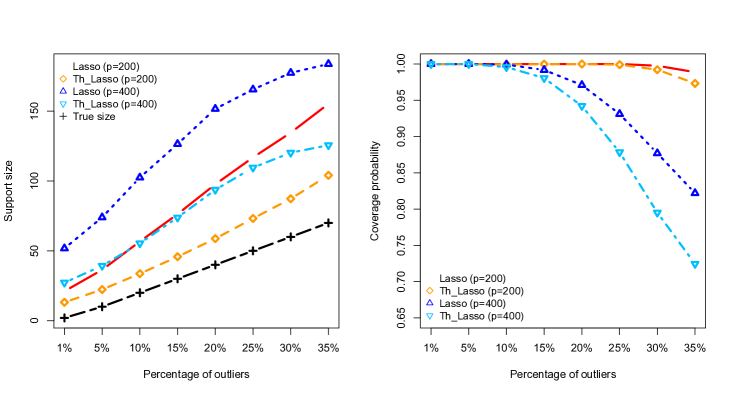
Figure 1: The support size (left) and the coverage probability (right) for the two preliminary estimators. “Lasso” means (3.7) and “Th_Lasso” means (3.11). Each point on the curve shows the mean based on 100 Monte Carlo simulations.

We examined numerical performances of our procedure based on 100 Monte Carlo simulations. All of the tuning parameters $\lambda_{\beta}$, $\lambda_{\gamma}$, $\lambda_{\theta}$ and $\tau_{\theta}$ were selected by the Bayesian information criteria (BIC; Schwarz (1978)). For instance, let us consider the selection of $(\lambda_{\beta},\lambda_{\gamma})$ by BIC. Let $\hat{\bm{\beta}}(\lambda_{\beta},\lambda_{\gamma})$ and $\hat{\bm{\gamma}}(\lambda_{\beta},\lambda_{\gamma})$ be the outputs of Algorithm 1 with the tuning parameters $(\lambda_{\beta},\lambda_{\gamma})$. Then, the optimal tuning parameters $(\hat{\lambda}_{\beta},\hat{\lambda}_{\gamma})$ are given by

$$(\hat{\lambda}_{\beta},\hat{\lambda}_{\gamma})=\mathop{\rm argmin}\limits_{\lambda_{\beta}>0;\lambda_{\gamma}>0} \frac{1}{2n}\|\bm{y}-\bm{X}\hat{\bm{\beta}}(\lambda_{\beta},\lambda_{\gamma})-\sqrt{n}\hat{\bm{\gamma}}(\lambda_{\beta},\lambda_{\gamma})\|_{2}^{2}$$

$$\qquad+\frac{\log n}{n}\big{\{}|{\rm supp}(\hat{\bm{\beta}}(\lambda_{\beta},\lambda_{\gamma}))|+|{\rm supp}(\hat{\bm{\gamma}}(\lambda_{\beta},\lambda_{\gamma}))|\big{\}}.$$

Practically, since it is impossible to search all possible tuning parameters, we searched them over some candidate values which were generated by the similar way to in Friedman et al. (2010).

The first two simulations were designed to see the impact of the number of outliers. The two scenarios $(n,p,s^{*})=(200,200,10)$ (moderate dimension) and $(n,p,s^{*})=(200,400,20)$ (high dimension) with various $g^{*}$ were considered. The covariates $\bm{x}_{i}$’s were independently drawn from $N_{p}(\bm{0},\bm{\Sigma})$ with $(\bm{\Sigma})_{ij}=0.3^{|i-j|}$, the true coefficients were given by $\beta_{j}^{*}={\rm sgn}(u_{j})$ and the true outliers were given by $\sqrt{n}\gamma_{i}^{*}=8$. The positions of the non-zero coefficients and outliers were uniformly drawn from $\{1,\dots,p\}$ and $\{1,\dots,n\}$, respectively. The $\varepsilon_{i}$’s and $u_{j}$’s were independently drawn from $N(0,1)$. Moreover, we used $R_{w}=100$ in (3.4) and Algorithm 1 stopped when $\|\bm{\beta}^{k}-\bm{\beta}^{k-1}\|_{1}/\tilde{s}\leq 10^{-3}$ was satisfied at the iteration $k$.

Pre.	Outlier	Criterion	Soft	Hard	SCAD	Garrote	Lasso	Oracle
(3.7)	5%	$\ell_{2}$-error	0.1036	0.1008	0.1026	0.1021	1.7400	0.3514
		FP	1.08	0.88	0.97	0.95	66.86	5.17
		TP	10.00	10.00	10.00	10.00	10.00	10.00
	10%	$\ell_{2}$-error	0.1059	0.1058	0.0992	0.1014	9.4954	-
		FP	1.27	1.09	1.07	1.11	124.53	-
		TP	10.00	10.00	10.00	10.00	9.97	-
	20%	$\ell_{2}$-error	0.1828	0.1436	0.1377	0.1485	32.0149	-
		FP	3.26	2.38	2.62	2.74	153.42	-
		TP	10.00	10.00	10.00	10.00	9.76	-
	30%	$\ell_{2}$-error	0.6788	0.4886	0.4683	0.5107	52.2651	-
		FP	6.77	5.04	5.33	5.68	157.06	-
		TP	9.87	9.89	9.89	9.89	9.53	-
(3.11)	5%	$\ell_{2}$-error	0.1067	0.1060	0.1059	0.1061	-	-
		FP	1.05	1.07	1.07	1.07	-	-
		TP	10.00	10.00	10.00	10.00	-	-
	10%	$\ell_{2}$-error	0.1097	0.1080	0.1084	0.1083	-	-
		FP	1.18	1.09	1.10	1.10	-	-
		TP	10.00	10.00	10.00	10.00	-	-
	20%	$\ell_{2}$-error	0.1654	0.1501	0.1487	0.1541	-	-
		FP	1.14	1.11	1.06	1.11	-	-
		TP	10.00	10.00	10.00	10.00	-	-
	30%	$\ell_{2}$-error	0.6583	0.5377	0.5502	0.5788	-	-
		FP	3.66	2.91	2.87	3.20	-	-
		TP	9.84	9.84	9.84	9.84	-	-

Table 1: Numerical performances of the proposed procedure for various outlier percentages when $(n,p,s^{*})=(200,200,10)$. Each value shows the mean based on 100 Monte Carlo simulations.

Figure 1 shows the support size $\tilde{s}+\tilde{g}$ (left) and the coverage probability $\mathbb{P}(S^{*}\subset\tilde{S},G^{*}\subset\tilde{G})$ (right) for the two preliminary estimators (3.7) and (3.11) when the percentage of outliers increases from 1% to 35%. It can be seen that the two preliminary estimators performed well if the percentage of outliers was lower than around 20%. The threshold version (3.11) had a smaller support size than (3.7), but its coverage probability was worse. We also notice that the coverage probability tended to be low as the percentage of outliers increased. It would come from the violation of the condition (3.3). As the number of outliers increases, the order $a_{n,1}$ increases.

Pre.	Outlier	Criterion	Soft	Hard	SCAD	Garrote	Lasso	Oracle
(3.7)	5%	$\ell_{2}$-error	0.2287	0.2139	0.2041	0.2087	3.8340	1.0337
		FP	2.32	2.05	2.04	2.09	97.95	21.69
		TP	20.00	20.00	20.00	20.00	19.98	20.00
	10%	$\ell_{2}$-error	0.3987	0.3096	0.3039	0.3218	8.5953	-
		FP	6.03	5.02	5.33	5.30	134.80	-
		TP	20.00	20.00	20.00	20.00	19.87	-
	20%	$\ell_{2}$-error	3.9041	3.5611	3.5540	3.6990	19.5640	-
		FP	21.51	18.74	19.77	20.44	158.11	-
		TP	19.01	18.99	19.00	19.09	18.79	-
	30%	$\ell_{2}$-error	13.7451	13.0448	13.7788	13.9348	30.6065	-
		FP	43.13	40.86	42.78	43.41	169.16	-
		TP	15.85	15.81	15.90	15.82	17.52	-
(3.11)	5%	$\ell_{2}$-error	0.2502	0.2280	0.2232	0.2293	-	-
		FP	2.17	2.06	1.98	2.10	-	-
		TP	20.00	20.00	20.00	20.00	-	-
	10%	$\ell_{2}$-error	0.4013	0.3253	0.3137	0.3345	-	-
		FP	2.91	2.43	2.57	2.56	-	-
		TP	19.99	19.99	19.99	19.99	-	-
	20%	$\ell_{2}$-error	4.1649	4.0372	3.9793	4.0969	-	-
		FP	19.78	19.04	18.81	19.04	-	-
		TP	18.99	19.01	19.00	19.00	-	-
	30%	$\ell_{2}$-error	13.2793	13.9873	13.7711	14.3158	-	-
		FP	41.10	41.02	41.00	41.39	-	-
		TP	16.02	16.03	15.99	16.00	-	-

Table 2: Numerical performances of the proposed procedure for various outlier percentages when $(n,p,s^{*})=(200,400,20)$.

Tables 1 and 2 show the squared $\ell_{2}$-error $\|\hat{\bm{\beta}}-\bm{\beta}^{*}\|_{2}^{2}$, the number of the false positives $|\{j|\beta_{j}^{*}=0,\hat{\beta}_{j}\neq 0\}|$ (FP) and the number of the true positives $|\{j|\beta_{j}^{*}\neq 0,\hat{\beta}_{j}\neq 0\}|$ (TP) for various penalties for outlier parameters. We used the preliminary estimator for $\bm{\beta}^{init}$ in Algorithm 1. We considered the “Soft”, “Hard”, “SCAD”, and “Garotte” thresholding functions. Only the Soft does not have the redescending property. The Garrote has a different behavior from the Hard and the SCAD, in fact, its $\psi(z;\lambda)$ function never vanishes if $z$ is finite. For the comparison, we also investigated the performances of the standard “Lasso” and its “Oracle” version where the true outliers are excluded in advance. The symbol “-” means that the standard Lasso does not depend on preliminary estimators and its oracle version does not so on outliers additionally.

As seen in Table 1, for the moderate dimension, our procedure provided quite good estimates and recovered the true support well. Interestingly, the performance was better than the Oracle. This would be because the error $\bm{\varepsilon}$ can yield extreme values in the simulation and the Oracle is not robust against these values. As seen in Table 2, however, for the high dimension and large outlier percentages, our procedure did not exhibit good performances. This result would come from the bad coverage probability of the preliminary estimators. Compared between the preliminary estimators, (3.11) performed better than (3.7) for the true support recovery, but the opposite was true for the $\ell_{2}$-error. It is also noted that the Soft performed worse than the other thresholding functions. This would be explained by the redescending property.

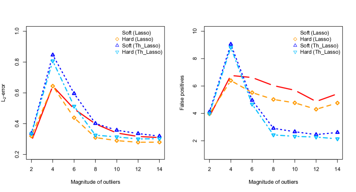
Figure 2: The squared $\ell_{2}$-error (left) and the false positives (right) for various magnitudes of outliers. Each point on the curve shows the mean based on 100 Monte Carlo simulations.

The final simulations are designed to investigate the impact of the magnitude of outliers. We used $(n,p,s^{*})=(200,400,20)$ with $g^{*}=20$ (10% outliers) and various magnitudes of $\sqrt{n}\bm{\gamma}^{*}$. We considered the situations $\sqrt{n}\bm{\gamma}^{*}=\gamma^{*}\bm{1}_{n}$ with $\gamma^{*}\in\{2,4,6,\dots,14\}$. The Monte Carlo samples were generated by the same way as above. In Figure 2, only the performances of the Soft and Hard are shown. The SCAD and Garotte performed similarly to the Hard. The true positives are also omitted since they were around 20 for all the cases considered. Our procedure performed well with low and high magnitudes, but it did not so with a moderate magnitude. This also would be come from the violation of the condition (3.3). For a low magnitude, the outliers would be hidden by the random errors. When $\bm{\varepsilon}$ is drawn from $N_{n}(\bm{0},\bm{I}_{n})$, the maximum magnitude of $\varepsilon_{i}$’s is less than $\sqrt{2\log n}$ (it is around 3.3 in this case). We also note that the performances tended to be stable as the magnitude increased.

5. Proofs

5.1. Proof of Proposition 1

Let $(\hat{\bm{\beta}},\hat{\bm{\gamma}})$ be the output of Algorithm 1. Then, from (2.3), we have for $j=1,\dots,p,$

$$\frac{1}{n}\sum_{i=1}^{n}x_{ij}(y_{i}-\bm{x}_{i}^{T}\hat{\bm{\beta}}-\sqrt{n}\hat{\gamma}_{i})+\lambda_{\beta,j}\partial|\hat{\beta}_{j}|=0.$$

Since $\psi(z;\lambda)=z-\Theta(z;\lambda)$, it follows from (2.4) that

$$\frac{1}{n}\sum_{i=1}^{n}x_{ij}(y_{i}-\bm{x}_{i}^{T}\hat{\bm{\beta}}-\sqrt{n}\hat{\gamma}_{i}) =\frac{1}{n}\sum_{i=1}^{n}x_{ij}(y_{i}-\bm{x}_{i}^{T}\hat{\bm{\beta}}-\Theta(y_{i}-\bm{x}_{i}^{T}\hat{\bm{\beta}};\lambda_{\gamma}w_{\gamma,i}))$$

$$=\frac{1}{n}\sum_{i=1}^{n}x_{ij}\psi(y_{i}-\bm{x}_{i}^{T}\hat{\bm{\beta}};\lambda_{\gamma}w_{\gamma,i}),$$

which ends the proof.

5.2. Proof of Theorem 1

To prove the theorem we prepare the next lemma.

Lemma 1.

Let $Z_{1},\dots,Z_{n}$ be independently identically distributed as the zero mean sub-Gaussian distribution with a parameter $\sigma>0$. Then, for any vector $\bm{a}\in\mathbb{R}^{n}$ and any $t\geq 0$,

$$\mathbb{P}\bigg{(}\bigg{|}\sum_{i=1}^{n}a_{i}Z_{i}\bigg{|}>t\bigg{)}\leq 2\exp\bigg{(}-\frac{t^{2}}{2\sigma^{2}\|\bm{a}\|_{2}^{2}}\bigg{)}.$$

Proof. Let $Z=\sum_{i=1}^{n}a_{i}Z_{i}$. From the Markov’s inequality, we have for $u>0$

$$\mathbb{P}\bigg{(}Z>t\bigg{)}=\mathbb{P}(e^{uZ}>e^{ut})\leq e^{-ut}\prod_{i=1}^{n}\mathbb{E}(e^{ua_{i}Z_{i}})\leq\exp\bigg{(}-ut+\frac{u^{2}\sigma^{2}\|\bm{a}\|_{2}^{2}}{2}\bigg{)}.$$

Note that $u=t/(\sigma^{2}\|\bm{a}\|_{2}^{2})$ minimizes $-ut+u^{2}\sigma^{2}\|\bm{a}\|_{2}^{2}/2$ over $u>0$. Thus, $\mathbb{P}(Z>t)\leq\exp\{-t^{2}/(2\sigma^{2}\|\bm{a}\|_{2}^{2})\}$. Similarly, $\mathbb{P}(Z<-t)\leq\exp\{-t^{2}/(2\sigma^{2}\|\bm{a}\|_{2}^{2})\}$ and then from $P(|Z|>t)\leq P(Z>t)+P(Z<-t)$ we obtain the lemma. ∎

Since we consider the adaptive Lasso type estimator and the screening property that $S^{*}\subset\tilde{S}$ and $G^{*}\subset\tilde{G}$ is satisfied under Condition 3 and (3.3), it suffices to focus only on the covariates selected by the preliminary estimator $\tilde{\bm{\beta}}$, that is, on the sub-matrix $\bm{X}_{\tilde{S}}=\{x_{ij}|\;1\leq i\leq n;j\in\tilde{S}\}$. Correspondingly, we only focus on the coefficients in the set $\tilde{S}$. In this section we omit the subscript $\tilde{S}$ for simplicity, therefore keep in mind that all of the following $\bm{X}$, $\bm{\beta}^{k}$ and $\bm{\beta}^{*}$ have the $\tilde{s}$ dimension.

We shall show the bound (3.5) on the event that Condition 3 is satisfied and on

$$E=\bigg{\{}\bigg{\|}\frac{1}{n}\bm{X}^{T}_{(\tilde{G}^{c})}\bm{\varepsilon}_{\tilde{G}^{c}}\bigg{\|}_{\infty}\leq C\sqrt{\frac{\sigma^{2}\log p}{n}}\bigg{\}}$$ (5.1)

both of which have probabilities going to one, where $\bm{X}_{(\tilde{G}^{c})}=\{x_{ij}|\;i\in\tilde{G}^{c},j\in\tilde{S}\}$, $\bm{\varepsilon}_{\tilde{G}^{c}}=\{\varepsilon_{i}|\;i\in\tilde{G}^{c}\}$ and $C>\sqrt{2}$. In fact, from Lemma 1 and Condition 1, we have for given the preliminary estimators $\tilde{\bm{\beta}}$ and $\tilde{\bm{\gamma}}$,

$$\mathbb{P}(E) =1-\mathbb{P}(E^{c})=1-\mathbb{P}\bigg{\{}\bigg{\|}\frac{1}{n}\bm{X}^{T}_{(\tilde{G}^{c})}\bm{\varepsilon}_{\tilde{G}^{c}}\bigg{\|}_{\infty}>C\sqrt{\frac{\sigma^{2}\log p}{n}}\bigg{\}}$$

$$\geq 1-\sum_{j\in\tilde{S}}\mathbb{P}\bigg{(}\bigg{|}\frac{1}{n}\sum_{i\in\tilde{G}^{c}}x_{ij}\varepsilon_{i}\bigg{|}>C\sqrt{\frac{\sigma^{2}\log p}{n}}\bigg{)}$$

$$\geq 1-2\sum_{j\in\tilde{S}}\exp(-2^{-1}C^{2}\log p)$$

$$\geq 1-2\exp(\log p-2^{-1}C^{2}\log p)=1-o(1).$$

Note that the lower bound does not depend on the preliminary estimators, and hence the probability of $E$ goes to one.

Since $\bm{\beta}^{k}={\rm argmin}_{\bm{\beta}}L(\bm{\beta},\bm{\gamma}^{k-1})$, it follows that $L(\bm{\beta}^{k},\bm{\gamma}^{k-1})\leq L(\bm{\beta}^{*},\bm{\gamma}^{k-1})$. Hence, we have

$$\frac{1}{2n}\|\bm{X}\bm{\Delta}^{k}\|_{2}^{2} \leq\frac{1}{n}\langle\bm{X}^{T}(\bm{y}-\bm{X}\bm{\beta}^{*}-\sqrt{n}\bm{\gamma}^{k-1}),\bm{\Delta}^{k}\rangle+\lambda_{\beta}\sum_{j\in\tilde{S}}w_{\beta,j}(|\beta_{j}^{*}|-|\beta_{j}^{k}|)$$

$$=A_{1}+A_{2},\quad{\rm say},$$

where $\bm{\Delta}^{k}=\bm{\beta}^{k}-\bm{\beta}^{*}$. First, we evaluate the term $A_{1}$. Since $\sqrt{n}\gamma_{i}^{k-1}=\Theta(y_{i}-\bm{x}_{i}^{T}\bm{\beta}^{k-1};\lambda_{\gamma}w_{\gamma,i})$ and $\sqrt{n}\gamma_{i}^{k-1}=0$ when $i\in\tilde{G}^{c}$, the $j$-th element of $\bm{X}^{T}(\bm{y}-\bm{X}\bm{\beta}^{*}-\sqrt{n}\bm{\gamma}^{k-1})$ is given by

$$\sum_{i\in\tilde{G}}x_{ij}\{y_{i}-\bm{x}_{i}^{T}\bm{\beta}^{*}-\Theta(y_{i}-\bm{x}_{i}^{T}\bm{\beta}^{k-1};\lambda_{\gamma}w_{\gamma,i})\}+\sum_{i\in\tilde{G}^{c}}x_{ij}(y_{i}-\bm{x}_{i}^{T}\bm{\beta}^{*})$$

$$\quad=\sum_{i\in\tilde{G}}x_{ij}\big{\{}\bm{x}_{i}^{T}\bm{\Delta}^{k-1}+(y_{i}-\bm{x}_{i}^{T}\bm{\beta}^{k-1})-\Theta(y_{i}-\bm{x}_{i}^{T}\bm{\beta}^{k-1};\lambda_{\gamma}w_{\gamma,i})\big{\}}$$

$$\qquad\qquad+\sum_{i\in\tilde{G}^{c}}x_{ij}(y_{i}-\bm{x}_{i}^{T}\bm{\beta}^{*}).$$

Thus, we obtain

$$A_{1} =\frac{1}{n}(\bm{X}_{(\tilde{G})}\bm{\Delta}^{k-1})^{T}(\bm{X}_{(\tilde{G})}\bm{\Delta}^{k})$$

$$\quad+\frac{1}{n}\sum_{j\in\tilde{S}}\Delta_{j}^{k}\sum_{i\in\tilde{G}}x_{ij}\{(y_{i}-\bm{x}_{i}^{T}\bm{\beta}^{k-1})-\Theta(y_{i}-\bm{x}_{i}^{T}\bm{\beta}^{k-1};\lambda_{\gamma}w_{\gamma,i})\}$$

$$\quad+\frac{1}{n}\sum_{j\in\tilde{S}}\Delta_{j}^{k}\sum_{i\in\tilde{G}^{c}}x_{ij}(y_{i}-\bm{x}_{i}^{T}\bm{\beta}^{*})=A_{11}+A_{12}+A_{13},\quad{\rm say}.$$

Since $\|\bm{\Delta}^{k}\|_{0}\leq\tilde{s}$ for any $k\geq 1$, the definition of the (doubly) restricted largest eigenvalue in (3.2) implies that

$$|A_{11}|\leq\frac{1}{n}\|\bm{X}_{(\tilde{G})}\bm{\Delta}^{k-1}\|_{2}\|\bm{X}_{(\tilde{G})}\bm{\Delta}^{k}\|_{2}\leq\delta_{max}(\tilde{s},\tilde{g})\|\bm{\Delta}^{k-1}\|_{2}\|\bm{\Delta}^{k}\|_{2}.$$ (5.2)

Note that $|\Theta(x;\lambda)-x|\leq\lambda$ under Condition 2. Then,

$$|A_{12}|\leq\frac{R_{w}\lambda_{\gamma}}{n}\|\bm{X}_{(\tilde{G})}\|_{\ell_{1}}\|\bm{\Delta}^{k}\|_{1}\leq C\sqrt{\frac{\sigma^{2}\log p}{n}}\|\bm{\Delta}^{k}\|_{1},$$ (5.3)

where $R_{w}>0$ is defined in (3.4). Since $G^{*}\subset\tilde{G}$, we have $\gamma_{i}^{*}=0$ for $i\in\tilde{G}^{c}$. Then, from (5.1), we have

$$|A_{13}|\leq\frac{1}{n}\|\bm{X}_{(\tilde{G}^{c})}\bm{\varepsilon}_{\tilde{G}^{c}}\|_{\infty}\|\bm{\Delta}^{k}\|_{1}\leq C\sqrt{\frac{\sigma^{2}\log p}{n}}\|\bm{\Delta}^{k}\|_{1}.$$ (5.4)

For the term $A_{2}$, since $S^{*}\subset\tilde{S}$,

$$A_{2} \leq\lambda_{\beta}\sum_{j\in S^{*}}w_{\beta,j}|\beta_{j}^{*}|-\lambda_{\beta}\sum_{j\in S^{*}}w_{\beta,j}|\beta_{j}^{*}+\Delta_{j}^{k}|-\lambda_{\beta}\sum_{j\in S^{*^{c}}}w_{\beta,j}|\beta_{j}^{*}+\Delta_{j}^{k}|$$

$$\leq\lambda_{\beta}\sum_{j\in S^{*}}w_{\beta,j}|\Delta_{j}^{k}|-\lambda_{\beta}\sum_{j\in S^{*^{c}}}w_{\beta,j}|\Delta_{j}^{k}|$$

$$\leq\lambda_{\beta}\max_{j\in S^{*}}w_{\beta,j}\|\bm{\Delta}_{S^{*}}^{k}\|_{1}-\frac{\lambda_{\beta}}{R_{w}}\|\bm{\Delta}_{S^{*^{c}}}^{k}\|_{1}$$

Combined with (5.2)–(5.4), it follows from $\|\bm{\Delta}^{k}\|_{1}=\|\bm{\Delta}_{S^{*}}^{k}\|_{1}+\|\bm{\Delta}_{S^{*c}}^{k}\|_{1}$ that

$$\frac{1}{2n}\|\bm{X}\bm{\Delta}^{k}\|_{2}^{2} \leq\delta_{max}(\tilde{s},\tilde{g})\|\bm{\Delta}^{k-1}\|_{2}\|\bm{\Delta}^{k}\|_{2}+2C\sqrt{\frac{\sigma^{2}\log p}{n}}\|\bm{\Delta}^{k}\|_{1}$$

$$\qquad+\lambda_{\beta}\max_{j\in S^{*}}w_{\beta,j}\|\bm{\Delta}_{S^{*}}^{k}\|_{1}-\frac{\lambda_{\beta}}{R_{w}}\|\bm{\Delta}_{S^{*c}}^{k}\|_{1}$$

$$=\delta_{max}(\tilde{s},\tilde{g})\|\bm{\Delta}^{k-1}\|_{2}\|\bm{\Delta}^{k}\|_{2}+\left(\lambda_{\beta}\max_{j\in S^{*}}w_{\beta,j}+2C\sqrt{\frac{\sigma^{2}\log p}{n}}\right)\|\bm{\Delta}^{k}_{S^{*}}\|_{1}$$

$$\qquad+\left(2C\sqrt{\frac{\sigma^{2}\log p}{n}}-\frac{\lambda_{\beta}}{R_{w}}\right)\|\bm{\Delta}_{S^{*c}}^{k}\|_{1}$$

$$\qquad\leq\delta_{max}(\tilde{s},\tilde{g})\|\bm{\Delta}^{k-1}\|_{2}\|\bm{\Delta}^{k}\|_{2}+\lambda_{\beta}\big{(}R_{w}^{-1}+\max_{j\in S^{*}}w_{\beta,j}\big{)}\sqrt{s^{*}}\|\bm{\Delta}^{k}\|_{2}.$$

From Condition 3 and (3.1), we have $\frac{1}{n}\|\bm{X}\bm{\Delta}^{k}\|_{2}^{2}\geq\kappa\|\bm{\Delta}^{k}\|_{2}^{2}$. Thus, for $k\geq 1$,

$$\|\bm{\Delta}^{k}\|_{2}\leq\rho\|\bm{\Delta}^{k-1}\|_{2}+2\kappa^{-1}\sqrt{s^{*}}\lambda_{\beta}\big{(}R_{w}^{-1}+\max_{j\in S^{*}}w_{\beta,j}\big{)}.$$

Let $\bm{\Delta}^{0}=\bm{\beta}^{init}-\bm{\beta}^{*}$. Then, the bound (3.5) is derived by solving the above recurrence relation for $k=1,2,\dots$, which ends the proof.

5.3. Proof of Theorem 2

Throughout this section we denote positive constants by $C_{i}\;(i\geq 1)$ which may be different from each other. Suppose that for some $\ell\in\tilde{S}\cap S^{*^{c}}$, $\beta_{\ell}^{k}\neq 0$. Without loss of generality, we can assume $\beta_{\ell}^{k}>0$. Then, from the first order condition for $\bm{\beta}^{k}$, the value

$$\frac{1}{n}\sum_{j\in\tilde{S}}\sum_{i=1}^{n}x_{ij}x_{i\ell}\beta_{j}^{k}-\frac{1}{n}\sum_{i=1}^{n}x_{i\ell}\bigg{\{}y_{i}-\Theta\big{(}y_{i}-\sum_{j\in\tilde{S}}x_{ij}\beta_{j}^{k-1};\lambda_{\gamma}w_{\gamma,i}\big{)}\bigg{\}}+\lambda_{\beta}w_{\beta,\ell}$$ (5.5)

should be zero. But, if we can show the first two terms are dominated by the third term $\lambda_{\beta}w_{\beta,\ell}$ for any $\ell\in\tilde{S}\cap S^{*^{c}}$, then the above value can never be zero, which leads to the contradiction.

First, we evaluate the middle term of (5.5). From the definition, the inside of $\Theta$ is represented as

$$y_{i}-\sum_{j\in\tilde{S}}x_{ij}\beta_{j}^{k-1}=\begin{cases}\sqrt{n}\gamma_{i}^{*}+\varepsilon_{i}-\sum_{j\in\tilde{S}}x_{ij}(\beta_{j}^{k-1}-\beta_{j}^{*}),&i\in G^{*}\cap\tilde{G}=G^{*}\\ \varepsilon_{i}-\sum_{j\in\tilde{S}}x_{ij}(\beta_{j}^{k-1}-\beta_{j}^{*}),&i\in G^{*^{c}}\cap\tilde{G}.\end{cases}$$

By Lemma 1, we can show that $\max_{1\leq i\leq n}|\varepsilon_{i}|\leq C_{1}\sqrt{\log n}$ with probability going to one. Let $\lambda_{\beta}=C_{2}\{(\log p)/n\}^{1/2}$, then it follows from Corollary 1 and $a_{n,2}s^{*}=o(n)$ that

$$\max_{1\leq i\leq n}\bigg{|}\varepsilon_{i}-\sum_{j\in\tilde{S}}x_{ij}(\beta_{j}^{k-1}-\beta_{j}^{*})\bigg{|} \leq\max_{1\leq i\leq n}|\varepsilon_{i}|+C_{3}\sqrt{\tilde{s}}\|\bm{\beta}^{k-1}-\bm{\beta}^{*}\|_{2}$$

$$\leq C_{4}\sqrt{\log n}(1+o(1)),$$

which implies that if $\lambda_{\gamma}\min_{i\in G^{*^{c}}\cap\tilde{G}}w_{\gamma,i}\geq C_{4}\sqrt{\log n}$, then $y_{i}-\sum_{j\in\tilde{S}}x_{ij}\beta_{j}^{k-1}=0$ for $i\in G^{*^{c}}\cap\tilde{G}$. Note that $\min_{i\in G^{*^{c}}\cap\tilde{G}}w_{\gamma,i}=R_{w}$ for sufficiently large $n$ since $\min_{i\in G^{*^{c}}\cap\tilde{G}}(1/|\tilde{\gamma}_{i}|)\geq 1/(Ca_{n,1})\to\infty$. Hence it suffices to put $\lambda_{\gamma}=C_{5}\sqrt{\log n}$ for a sufficiently large $C_{5}>0$. Such a $\lambda_{\gamma}$ satisfying the condition of Corollary 1 can be selected since $a_{n,2}^{2}=o(n)$. Meanwhile, since $\sqrt{\log n}=o(\sqrt{n}\min_{i\in G^{*}}|\gamma_{i}^{*}|)$, we have $y_{i}-\sum_{j\in\tilde{S}}x_{ij}\beta_{j}^{k-1}=\sqrt{n}\gamma_{i}^{*}(1+o(1))$ for $i\in G^{*}$. Thus, for sufficiently large $n$, it holds that $\min_{i\in G^{*}}|y_{i}-\sum_{j\in\tilde{S}}x_{ij}\beta_{j}^{k-1}|\geq\lambda_{\gamma}R_{w}\geq\lambda_{\gamma}\max_{i\in G^{*}}w_{\gamma,i}$. Therefore, under Condition 2,

$$\Theta\big{(}y_{i}-\sum_{j\in\tilde{S}}x_{ij}\beta_{j}^{k-1};\lambda_{\gamma}w_{\gamma,i}\big{)}=\begin{cases}y_{i}-\sum_{j\in\tilde{S}}x_{ij}\beta_{j}^{k-1}+O(\sqrt{\log n}),&i\in G^{*}\\ 0,&i\in G^{*^{c}}\cap\tilde{G}.\end{cases}$$

Then, it follows that

$$\sum_{i=1}^{n}x_{i\ell}\bigg{\{}y_{i}-\Theta\big{(}y_{i}-\sum_{j\in\tilde{S}}x_{ij}\beta_{j}^{k-1};\lambda_{\gamma}w_{\gamma,i}\big{)}\bigg{\}}$$

$$\qquad=\sum_{i\in\tilde{G}}x_{i\ell}\bigg{\{}y_{i}-\Theta\big{(}y_{i}-\sum_{j\in\tilde{S}}x_{ij}\beta_{j}^{k-1};\lambda_{\gamma}w_{\gamma,i}\big{)}\bigg{\}}+\sum_{i\in\tilde{G}^{c}}x_{i\ell}y_{i}$$

$$\qquad=\sum_{i\in G^{*}}x_{i\ell}\sum_{j\in\tilde{S}}x_{ij}\beta_{j}^{k-1}+O(\sqrt{\log n})\sum_{i\in G^{*}}x_{i\ell}+\sum_{i\in G^{*^{c}}\cap\tilde{G}}x_{i\ell}y_{i}+\sum_{i\in\tilde{G}^{c}}x_{i\ell}y_{i}$$

$$\qquad=\sum_{i\in G^{*}}x_{i\ell}\sum_{j\in\tilde{S}}x_{ij}\big{\{}\beta_{j}^{*}+(\beta_{j}^{k-1}-\beta_{j}^{*})\big{\}}+\sum_{i\in G^{*^{c}}}x_{i\ell}y_{i}+O(g^{*}\sqrt{\log n})$$

$$\qquad=\sum_{i=1}^{n}\sum_{j\in\tilde{S}}x_{i\ell}x_{ij}\beta_{j}^{*}+\sum_{i\in G^{*}}\sum_{j\in\tilde{S}}x_{i\ell}x_{ij}(\beta_{j}^{k-1}-\beta_{j}^{*})+\sum_{i\in G^{*^{c}}}x_{i\ell}\varepsilon_{i}+O(g^{*}\sqrt{\log n}).$$

Thus, (5.5) can be written as

$$\frac{1}{n}\sum_{i=1}^{n}\sum_{j\in\tilde{S}}x_{ij}x_{i\ell}(\beta_{j}^{k}-\beta_{j}^{*})-\frac{1}{n}\sum_{i\in G^{*}}\sum_{j\in\tilde{S}}x_{ij}x_{i\ell}(\beta_{j}^{k-1}-\beta_{j}^{*})$$

$$\qquad\qquad-\frac{1}{n}\sum_{i\in G^{*^{c}}}x_{i\ell}\varepsilon_{i}+O\bigg{(}\frac{g^{*}}{n}\sqrt{\log p}\bigg{)}+\lambda_{\beta}w_{\beta,\ell}.$$

Clearly the fist and second terms have the order $\sqrt{a_{n,2}s^{*}}\lambda_{\beta}$. From the proof of Theorem 1, the third term is of order $\{(\log p)/n\}^{1/2}$. By $a_{n,1}\max\big{(}\sqrt{a_{n,2}s^{*}},g^{*}/\sqrt{n}\big{)}=o(1)$, the first four terms of (5.5) are dominated by $\lambda_{\beta}\min_{j\in\tilde{S}\cap S^{*^{c}}}w_{\beta,j}$ since $\min_{j\in\tilde{S}\cap S^{*^{c}}}w_{\beta,j}\geq 1/(Ca_{n,1})$.

Acknowledgements

This work was supported by the System Genetics Project of the Research Organization of Information and Systems.

Tokyo Institute of Technology, Tokyo, Japan. E-mail: katayama.s.ad@m.titech.ac.jp

The Institute of Statistical Mathematics, Tokyo, Japan. E-mail: fujisawa@ism.ac.jp

References

• Antoniadis and Fan (2001) Antoniadis, A. and Fan, J. (2001). Regularization of wavelet approximations. Journal of the American Statistical Association 96, 939-967.
• Bickel et al. (2009) Bickel, P., Ritov, Y. and Tsybakov, A. (2009). Simultaneous analysis of lasso and dantzig selector. The Annals of Statistics 37, 1705-1732.
• Efron et al. (2004) Efron B., Hastie, T., Johnstone, I. and Tibshirani, R. (2004). Least angle regression (with Discussion). The Annals of Statistics 32, 407-499.
• Fan (1997) Fan, J. (1997). Comments on ‘wavelets in statistics: A review’ by A. Antoniadis. Journal of the American Statistical Association 6, 131-139.
• Fan and Li (2001) Fan, J. and Li, R. (2001). Variable selection via nonconcave penalized likelihood and its oracle properties. Journal of the American Statistical Association 96, 1348-1360.
• Fan and Lv (2013) Fan, Y. and Lv, J. (2013). Asymptotic equivalence of regularization methods in thresholded parameter space. Journal of the American Statistical Association 108, 1044-1061.
• Fan and Lv (2014) Fan, Y. and Lv, J. (2014). Asymptotic properties for combined $L_{1}$ and concave regularization. Biometrika 101, 57-70.
• Friedman et al. (2010) Friedman, J., Hastie, T. and Tibshirani, R. (2010). Regularization paths for generalized linear models via coordinate descent. Journal of Statistical Software 33, 1-22.
• Gao (1998) Gao, H. (1998). Wavelet shrinkage denoising using the non-negative garrote. Journal of Computational and Graphical Statistics 7, 469-488.
• Huber and Ranchetti (2009) Huber, P. and Ronchetti, E. (2009). Robust statistics, 2nd edition. Wiley, New York.
• Meinshausen and Yu (2009) Meinshausen, N. and Yu, B. (2009). Lasso-type recovery of sparse representations for high-dimensional data. The Annals of Statistics 37, 246-270.
• Nguyen and Tran (2013) Nguyen, N. and Tran, T. (2013). Robust lasso with missing and grossly corrupted observations. IEEE Transactions Information Theory 59, 2036-2058.
• Schwarz (1978) Schwarz, G. (1978). Estimating the dimension of a model. The Annals of Statistics 6, 461-464.
• She and Owen (2011) She, Y. and Owen, A. (2011). Outlier detection using nonconvex penalized regression. Journal of the American Statistical Association 106, 626-639.
• Tibshirani (1996) Tibshirani, R. (1996). Regression shrinkage and selection via the lasso. Journal of Royal Statistical Society B 58, 267-288.
• van de Geer and Bühlmann (2009) Van De Geer, S. and Bühlmann, P. (2009). On the conditions used to prove oracle results for the Lasso. Electronic Journal of Statistics 3, 1360-1392.
• Vershynin (2012) Vershynin, R. (2012). Introduction to the non-asymptotic analysis of random matrices. Compressed Sensing, Theory and Applications 5, 210-268.
• Wainwright (2009) Wainwright, M. (2009). Sharp thresholds for high-dimensional and noisy sparsity recovery using $\ell_{1}$-constrained quadratic programming (lasso). IEEE Transactions Information Theory 55, 2183-2202.
• Zhang (2010) Zhang, C. (2010). Nearly unbiased variable selection under minimax concave penalty. The Annals of Statistics 38, 894-942.
• Zhang and Huang (2008) Zhang, C. and Huang, J. (2008). The sparsity and bias of the LASSO selection in high-dimensional linear regression. The Annals of Statistics 36, 1567-1594.
• Zhang and Zhang (2012) Zhang, C. and Zhang, T. (2012). A general theory of concave regularization for high-dimensional sparse estimation problems. Statistical Science 27, 576-593.
• Zhao and Yu (2006) Zhao, P. and Yu, B. (2006). On model selection consistency of Lasso. Journal of Machine Learning Research 7, 2541-2563.
• Zou (2006) Zou, H. (2006). The adaptive Lasso and its oracle properties. Journal of the American Statistical Association 101, 1418-1429.