On equivariant quantum Schubert calculus for $G/P$

Abstract.

We show a $\mathbb{Z}^{2}$-filtered algebraic structure and a “quantum to classical” principle on the torus-equivariant quantum cohomology of a complete flag variety of general Lie type, generalizing earlier works of Leung and the second author. We also provide various applications on equivariant quantum Schubert calculus, including an equivariant quantum Pieri rule for partial flag variety $F\ell_{n_{1},\cdots,n_{k};n+1}$ of Lie type $A$.

1. Introduction

The complex Grassmannian $Gr(m,n+1)$ parameterizes $m$-dimensional complex vector subspaces of $\mathbb{C}^{n+1}$. The integral cohomology ring $H^{*}(Gr(m,n+1),\mathbb{Z})$ has an additive basis of Schubert classes $\sigma^{\nu}$, indexed by partitions $\nu=(\nu_{1},\cdots,\nu_{m})$ inside an $m\times(n+1-m)$ rectangle: $n+1-m\geq\nu_{1}\geq\cdots\geq\nu_{m}\geq 0$. The initial classical Schubert calculus, in modern language, refers to the study of the ring structure of $H^{*}(Gr(m,n+1),\mathbb{Z})$. The content includes

1. a Pieri rule, giving a combinatorial formula for the cup product by a set of generators of the cohomology ring, for instance by the special Schubert classes $\sigma^{1^{p}}$, $1\leq p\leq m$, where $1^{p}=(1,\cdots,1,0,\cdots,0)$ has precisely $p$ copies of 1;

2. more generally, a Littlewood-Richardson rule, giving a (manifestly positive) combinatorial formula of the structure constants $N_{\mu,\nu}^{\eta}$ in the cup product $\sigma^{\mu}\cup\sigma^{\nu}=\sum_{\eta}N_{\mu,\nu}^{\eta}\sigma^{\eta}$;

3. a ring presentation of $H^{*}(Gr(m,n+1),\mathbb{Z})$;

4. a Giambelli formula, expressing every $\sigma^{\nu}$ as a polynomial in special Schubert classes.

The complex Grassmannian $Gr(m,n+1)$ is a special case of homogeneous varieties $G/P$, where $G$ denotes the adjoint group of a complex simple Lie algebra of rank $n$, and $P$ denotes a parabolic subgroup of $G$. The classical Schubert calculus, in general, refers to the study of the classical cohomology ring $H^{*}(G/P)=H^{*}(G/P,\mathbb{Z})$.

There are various extensions of the classical Schubert calculus by replacing “classical” with “equivariant”, “quantum”, or “equivariant quantum”. The equivariant quantum Schubert calculus for $G/P$ refers to the study of the (integral) torus-equivariant quantum cohomology ring $QH^{*}_{T}(G/P)$, which is a deformation of the ring structure of the torus-equivariant cohomology $H^{*}_{T}(G/P)$ by incorporating genus zero, three-point equivariant Gromov-Witten invariants. In analogy with $H^{*}(Gr(m,n+1))$, the ring $QH^{*}_{T}(G/P)$ has a basis of Schubert classes $\sigma^{u}$ over $H^{*}_{T}(\mbox{pt})[q_{1},\cdots,q_{k}]$ where $k:=\dim H_{2}(G/P)$, indexed by elements in a subset $W^{P}$ of the Weyl group $W$ of $G$. The structure coefficients $N_{u,v}^{w,\mathbf{d}}$ of the equivariant quantum product

$$\sigma^{u}\star\sigma^{v}=\sum_{w\in W^{P},\mathbf{d}\in H_{2}(G/P,\mathbb{Z})}N_{u,v}^{w,\mathbf{d}}\sigma^{w}q^{\mathbf{d}}$$

are homogeneous polynomials in $H_{T}^{*}(\mbox{pt})=\mathbb{Z}[\alpha_{1},\cdots,\alpha_{n}]$ with variables $\alpha_{i}$ being simple roots of $G$. They contain all the information in the former kinds of Schubert calculus. For instance, the non-equivariant limit of $N_{u,v}^{w,\mathbf{d}}$, given by evaluating $(\alpha_{1},\cdots,\alpha_{n})=\mathbf{0}$, recovers an ordinary Gromov-Witten invariant, which counts the number of degree $\mathbf{d}$ rational curves in $G/P$ passing through three Schubert subvarieties associated to $u,v$, $w$.

When $G=PSL(n+1,\mathbb{C})$, the Weyl group $W$ is a permutation group $S_{n+1}$ generated by transpositions $s_{i}=(i,i+1)$. Every homogenous variety $PSL(n+1,\mathbb{C})/P$ is of the form $F\ell_{n_{1},\cdots,n_{k};n+1}:=\{V_{n_{1}}\leqslant\cdots\leqslant V_{n_{k}}\leqslant\mathbb{C}^{n+1}~{}|~{}\dim_{\mathbb{C}}V_{n_{j}}=n_{j},\,\,\forall 1\leq j\leq k\}$, parameterizing partial flags in $\mathbb{C}^{n+1}$. As an algebra over $H_{T}^{*}(\mbox{pt})[q_{1},\cdots,q_{k}]$, the equivariant quantum cohomology ring $QH^{*}_{T}(F\ell_{n_{1},\cdots,n_{k};n+1})$ is generated (see e.g. [AnCh, LaSh-QDSP]) by special Schubert classes

$$\sigma^{c[n_{i},p]},\quad\mbox{where}\quad c[n_{i},p]:=s_{n_{i}-p+1}\cdots s_{n_{i}-1}s_{n_{i}}.$$

One of the main results of our present paper is the following equivariant quantum Pieri rule. The non-equivariant limit of it recovers the quantum Pieri rule, which was first given by Ciocan-Fontanine [CFon], and was reproved by Buch [Buch-PartialFlag]. The classical limit (by evaluating $\mathbf{q}=\mathbf{0}$) is a slight improvement of Robinson’s equivariant Pieri rule [Robinson]. By evaluating all equivariant parameters $\alpha_{i}$ and all quantum parameters $q_{j}$ at 0, we have the classical Pieri rule due to Lascoux and Schützenberger [LasSch] and Sottile [Sottile].

Theorem 3.10. For any $1\leq i\leq k,1\leq p\leq n_{i}$ and any $u\in W^{P}$, we have

$$\sigma^{c[n_{i},p]}\star\sigma^{u}=\sum_{\mathbf{d}\in\scriptsize\mbox{Pie}_{i,p}(u)}\sum_{j=0}^{p-d_{i}}\sum_{w}\xi^{n_{i}-d_{i}-j,p-d_{i}-j}(\mu_{w\cdot\phi_{\mathbf{d}},u\cdot\tau_{\mathbf{d}},n_{i}-d_{i}})\sigma^{w}q^{\mathbf{d}}$$

with the last summation over those $w\in\mbox{Per}(\mathbf{d})$ satisfying $w\cdot\phi_{\mathbf{d}}\in S_{n_{i}-d_{i},j}(u\cdot\tau_{\mathbf{d}})$.

Here $\mbox{Pie}_{i,p}(u)$, etc., are combinatorial sets to be described in section 3.1; the element $\mu=\mu_{w\cdot\phi_{\mathbf{d}},u\cdot\tau_{\mathbf{d}},n_{i}-d_{i}}$ is a partition inside an $(n_{i}-d_{i}-j)\times(n+1-n_{i}+d_{i}+j)$ rectangle. Each structure coefficient $\xi^{n_{i}-d_{i}-j,p-d_{i}-j}(\mu)$ coincides with the coefficient of $\sigma^{\mu}$ in the equivariant product $\sigma^{c[n_{i},p]}\circ\sigma^{\mu}$ in $H^{*}_{T}(Gr(n_{i}-d_{i}-j,n+1))$. Geometrically, it is the restriction of the Grassmannian Schubert class $\sigma^{(1^{p-d_{i}-j})}$ of $H^{*}_{T}(Gr(n_{i}-d_{i}-j,n+1))$ (labeled by the special partition of $(p-d_{i}-j)$ copies of 1) to a $T$-fixed point labeled by the partition $\mu$. These restriction type structure coefficients can be easily computed in many ways [KoKu, Billey, BuRi, KnutTao, Laksov, GaSa, Kreiman, ThYo]. For completeness, we will include a known formula in Definition 3.4. We remark that our formula above is different from the one in [LaSh-affinePieri] by Lam and Shimozono, which concerns the multiplications by $\sigma^{s_{p}s_{p-1}\cdots s_{2}s_{1}s_{\theta}}$ in the ring $QH^{*}_{T}(F\ell_{1,2,\cdots,n;n+1})$. Here $\theta$ denotes the highest root, and a ring isomorphism [Peterson, LaSh-GoverPaffineGr, LeungLi-GWinv] between $QH^{*}_{T}(F\ell_{1,2,\cdots,n;n+1})$ and the equivariant homology $H_{*}^{T}(\Omega SU(n+1))$ of based loop groups after localization is involved.

In the special case of complex Grassmannians, $H_{2}(Gr(m,n+1),\mathbb{Z})=\mathbb{Z}$, so that there is only one quantum variable $q$. Let $\mathcal{P}_{m,n+1}$ denote the set of partitions inside an $m\times(n+1-m)$ rectangle. For $\nu=(\nu_{1},\cdots,\nu_{m})$ and $\eta=(\eta_{1},\cdots,\eta_{m})$ in $\mathcal{P}_{m,n+1}$ satisfying $\eta_{i}-\nu_{i}\in\{0,1\}$ for all $i$, we introduce an associated partition $\eta_{\nu}\in\mathcal{P}_{m-r,n+1}$,

$$\eta_{\nu}:=(\nu_{j_{1}}-j_{1}+r+1,\nu_{j_{2}}-j_{2}+r+2,\cdots,\nu_{j_{m-r}}-j_{m-r}+m),$$

where $j_{1}<j_{2}<\cdots<j_{m-r}$ denote all entries with $\eta_{j_{i}}=\nu_{j_{i}}$. In other words, the Young diagram of $\eta$ is obtained by adding a vertical strip to the Young diagram of $\nu$; the associated partition $\eta_{\nu}$ can also described with this flavor by using a simple join-and-cut operation (see Definition 3.15 and the figures therein for more details). A further simplification of the above theorem leads to the following equivariant quantum Pieri rule for complex Grassmannians.

Theorem 3.17. Let $1\leq p\leq m$ and $\nu=(\nu_{1},\cdots,\nu_{m})\in\mathcal{P}_{m,n+1}$. In $QH^{*}_{T}(Gr(m,n+1))$,

$$\sigma^{1^{p}}\star\sigma^{\nu}=\sum_{r=0}^{p}\sum_{\eta}\xi^{m-r,p-r}(\eta_{\nu})\sigma^{\eta}+\sum_{r=0}^{p-1}\sum_{\kappa}\xi^{m-1-r,p-1-r}(\kappa^{\prime}_{\nu^{\prime}})\sigma^{\kappa}q,$$

where the second sum is over partitions $\eta=(\eta_{1},\cdots,\eta_{m})\in\mathcal{P}_{m,n+1}$ satisfying $|\eta|=|\nu|+r$ and $\eta_{i}-\nu_{i}\in\{0,1\}$ for all $i$; the $q$-terms occur only if $\nu_{1}=n+1-m$, and when this holds, the last sum is over partitions $\kappa=(\kappa_{1},\cdots,\kappa_{m-1},0)$ such that $\kappa^{\prime}:=(\kappa_{1}+1,\cdots,\kappa_{m-1}+1)$ and $\nu^{\prime}:=(\nu_{2},\cdots,\nu_{m})$ satisfy $|\kappa^{\prime}|=|\nu^{\prime}|+r$ and $\kappa_{i}+1-\nu_{i+1}\in\{0,1\}$ for all $1\leq i\leq m-1$.

For instance in $QH^{*}_{T}(Gr(3,7))$, we have

$$\sigma^{(1,1,1)}\star\sigma^{(4,0,0)}=(\alpha_{1}+\cdots+\alpha_{6})\sigma^{(4,1,1)}+q.$$

The special case when $p=1$ has been given by Mihalcea [Miha-EQSC]. The full Pieri-type formula could have been obtained by combining the study of the equivariant quantum K-theory [BuMi-quantumKtheory] with an equivariant Pieri rule [Laksov, GaSa] using Grassmannian algebras. It might also be deduced by the results in [LaSh-GoverPaffineGr, LaSh-affinePieri]. However, an explicit statement, which is a very important component of the equivariant quantum Schubert calculus, has not been given anywhere else yet. Actually, the equivariant Pieri rule, which is read off from the classical part of Theorem 3.17, is different from the aforementioned known formulations. It has even inspired the second author and Ravikumar to find an equivariant Pieri rule for Grassmannians of all classical Lie types with a geometric approach in their recent work [LiRa]. On the other hand, Buch has recently shown a (manifestly positive) equivariant puzzle rule for two-step flag varieties [Buch-equivTwostep], generalizing the rules in [KnutTao, BKPT]. Therefore he obtains a Littlewood-Richardson rule for $QH^{*}_{T}(Gr(m,n+1))$, due to the equivariant “quantum to classical” principle [BuMi-quantumKtheory]. It will be interesting to study how we simplify Buch’s general rule in the special case of Pieri rule to obtain a more compact form as above.

In analogy with the contents (1),(2),(3),(4) of the classical Schubert calculus, there are the corresponding equivariant quantum extensions, say $(1)^{\prime},(2)^{\prime},(3)^{\prime}$ and $(4)^{\prime}$, in the equivariant quantum Schubert calculus. The problem $(2)^{\prime}$ of finding a manifestly positive formula of the structure constants for the equiavariant quantum cohomology remains open except for very few cases including complex Grassmannians [Buch-equivTwostep] (which is widely open even for the classical Schubert calculus). For $(3)^{\prime}$ and $(4)^{\prime}$, there have been a few developments (see [Kim-EquiQH] and [LaSh-QDSP, AnCh, IMN] respectively). For $QH^{*}_{T}(F\ell_{n_{1},\cdots,n_{k};n+1})$, we expect that our Theorem 3.10 leads to an alternative approach to the earlier studies on $(3)^{\prime}$ and $(4)^{\prime}$. Indeed, we will illustrate this for the special case of complex Grassmannians [Mihalcea-EQGiambelli], by using Theorem 3.17.

It is another one of the main results of the present paper that the “quantum to classical” principle holds among various equivariant Gromov-Witten invariants of $G/P$. Applying it for $G=PSL(n+1,\mathbb{C})$, we achieve the above theorems. In [LeungLi-functorialproperties, Li-functorial], Leung and the second author discovered a functorial relationship between the quantum cohomologies of complete and partial flag varieties, in terms of filtered algebraic structures on $QH^{*}(G/B)$. A “quantum to classical” principle among various Gromov-Witten invariants of $G/B$ was therefore obtained [LeungLi-QuantumToClassical] in a combinatorial way. Such a principle was also shown for some other cases [BKT-GWinv, CMP-I, ChPe] in a geometric way. It has led to nice applications in finding Pieri-type formulas, such as [BKT-Isotropic, LeungLi-QPR]. In the present paper, we generalize the work [LeungLi-functorialproperties] to the equivariant quantum cohomology $QH^{*}_{T}(G/B)$ in the following case.

Theorem 2.5. Let $P\supset B$ be a parabolic subgroup of $G$ such that $P/B$ is isomorphic to the complex projective line $\mathbb{P}^{1}$. With respect to the natural projection $G/B\to G/P$, there is a $\mathbb{Z}^{2}$-filtration $\mathcal{F}=\{F_{\mathbf{a}}\}$ on $QH^{*}_{T}(G/B)$ respecting the algebra structure: $F_{\mathbf{a}}\star F_{\mathbf{b}}\subset F_{\mathbf{a}+\mathbf{b}}$ for any $\mathbf{a},\mathbf{b}\in\mathbb{Z}^{2}$. Moreover, the associated graded algebra $Gr^{\mathcal{F}}(QH^{*}_{T}(G/B))$ is isomorphic to $QH^{*}(P/B)\otimes_{\mathbb{Z}}QH^{*}_{T}(G/P)$ as $\mathbb{Z}^{2}$-graded $\mathbb{Z}$-algebras, after localization.

Explicit construction of the $\mathbb{Z}^{2}$-filtration will be given in section 2.2. As a consequence, we obtain Theorem 2.7, giving identities among various equivariant Gromov-Witten invariants of $G/B$. This is an extension of Theorem 1.1 [LeungLi-QuantumToClassical] in exactly the same form. Together with an equivariant extension of Peterson-Woodward comparison formula (see Proposition 2.10), we expect that Theorem 2.7 leads to nice applications in the equivariant quantum Schubert calculus for various $G/P$. Indeed, for $G=PSL(n+1,\mathbb{C})$, we can reduce all the relevant equivariant Gromov-Witten invariants in Theorem 3.10 to Pieri-type structure coefficients for $H^{*}_{T}(F\ell_{1,2,\cdots,n;n+1})$, by applying Theorem 2.7 repeatedly. Combining such reductions with Robinson’s equivariant Pieri rule [Robinson], we obtain Theorem 3.10. It will be very interesting to explore a simpler and conceptually much cleaner proof by a kind of inductive argument based on Mihalcea’s characterization of the structure coefficients via the equivariant quantum Chevalley rule [Miha-EQCRandCri]. We can also find nice applications on the equivariant quantum Pieri rules for orthogonal isotropic Grassmannians, in a joint work in progress by the second author and Ravikumar.

This paper is organized as follows. In section 2, we introduce basic notations, and prove the main technical results for homogeneous varieties $G/P$ of general Lie type. In section 3, we show an equivariant quantum Pieri rule for $F\ell_{n_{1},\cdots,n_{k};n+1}$, and give a simplification in the special case of complex Grassmannians. Finally in the appendix, we give alternative proofs of a ring presentation of $QH^{*}_{T}(Gr(m,n+1))$ and the equivariant quantum Giambelli formula for $Gr(m,n+1)$.

Acknowledgements

The authors thank Leonardo Constantin Mihalcea for his generous helps. The authors also thank Anders Skovsted Buch, Ionut Ciocan-Fontanine, Thomas Lam, and Naichung Conan Leung for helpful conversations. The authors would like to thank the anonymous referees for their valuable comments on an earlier version of the manuscript. The second author is supported by IBS-R003-D1.

2. A $\mathbb{Z}^{2}$-filtration on $QH^{*}_{T}(G/B)$ and its consequences

In this section, we show a $\mathbb{Z}^{2}$-filtered algebraic structure on $QH^{*}_{T}(G/B)$, with respect to a choice of a simple root. We also obtain a number of identities among various equivariant Gromov-Witten invariants of $G/B$.

2.1. Preliminaries

We fix the notions here, following [Hump-LieAlg, Hump-AlgGroup, FuPa].

Let $\mathfrak{g}$ be a complex simple Lie algebra of rank $n$, $\mathfrak{h}$ be a Cartan subalgebra of $\mathfrak{g}$, and $\Delta=\{\alpha_{1},\cdots,\alpha_{n}\}\subset\mathfrak{h}^{*}$ be a basis of simple roots. Let $R$ denote the root system of $(\mathfrak{g},\mathfrak{h})$. We have $R=R^{+}\sqcup(-R^{+})$ with $R^{+}=R\cap\bigoplus_{i=1}^{n}{\mathbb{Z}_{\geq 0}}\alpha_{i}$ called the set of positive roots, and have the Cartan decomposition $\mathfrak{g}=\mathfrak{h}\bigoplus\big{(}\bigoplus_{\gamma\in R}\mathfrak{g}_{\gamma}\big{)}$. Let $G$ be the (connected) adjoint group of $\mathfrak{g}$, and $B\subset G$ be the Borel subgroup with $\mathfrak{b}:=\mbox{Lie}(B)=\mathfrak{h}\bigoplus(\bigoplus_{\gamma\in R^{+}}\mathfrak{g}_{\gamma}\big{)}$. Each subset $\Delta^{\prime}$ of $\Delta$ gives a root subsystem $R_{\Delta^{\prime}}=R^{+}_{\Delta}\sqcup(-R^{+}_{\Delta^{\prime}})$ where $R_{\Delta^{\prime}}^{+}=R^{+}\bigcap\big{(}\bigoplus_{\alpha\in\Delta^{\prime}}\mathbb{Z}\alpha\big{)}$, and defines a parabolic subalgebra by $\mathfrak{p}(\Delta^{\prime}):=\mathfrak{b}\bigoplus\big{(}\bigoplus_{\gamma\in-R^{+}_{\Delta^{\prime}}}\mathfrak{g}_{\gamma}\big{)}$. This gives rise to a one-to-one correspondence between the subsets $\Delta_{P}$ of $\Delta$ and the parabolic subgroups $P\subset G$ that contain $B$. In particular, we denote by $P_{\beta}$ the parabolic subgroup corresponding to a subset $\{\beta\}\subset\Delta$. We notice that $P_{\beta}$ is a minimal subgroup among those parabolic subgroups $P\supsetneq B$, and $P_{\beta}/B$ is isomorphic to the complex projective line $\mathbb{P}^{1}$.

Let $\{\alpha_{1}^{\vee},\cdots,\alpha_{n}^{\vee}\}\subset\mathfrak{h}$ be the simple coroots, $\{\chi_{1}^{\vee},\cdots,\chi_{n}^{\vee}\}\subset\mathfrak{h}$ be the fundamental coweights, $\{\chi_{1},\cdots,\chi_{n}\}\subset\mathfrak{h}^{*}$ be the fundamental weights, and $\rho:=\sum_{i=1}^{n}\chi_{i}$. Let $\langle\cdot,\cdot\rangle:\mathfrak{h}^{*}\times\mathfrak{h}\rightarrow\mathbb{C}$ denote the natural pairing. Every simple root $\alpha_{i}$ labels a simple reflection $s_{i}:=s_{\alpha_{i}}$, which maps $\lambda\in\mathfrak{h}$ and $\gamma\in\mathfrak{h}^{*}$ to $s_{i}(\lambda)=\lambda-\langle\alpha_{i},\lambda\rangle\alpha_{i}^{\vee}$ and $s_{i}(\gamma)=\gamma-\langle\gamma,\alpha_{i}^{\vee}\rangle\alpha_{i}$ respectively. Let $W$ denote the Weyl group generated by all the simple reflections, and $W_{P}$ denote the subgroup of $W$ generated by $\{s_{\alpha}~{}|~{}\alpha\in\Delta_{P}\}$. Let $\ell:W\rightarrow\mathbb{Z}_{\geq 0}$ denote the standard length function, $\omega$ (resp. $\omega_{P}$) denote the longest element in $W$ (resp. $W_{P}$), and $W^{P}$ denote the subset of $W$ that consists of minimal length representatives of the cosets in $W/W_{P}$. Denote $Q^{\vee}:=\bigoplus_{i=1}^{n}\mathbb{Z}\alpha_{i}^{\vee}$ and $Q^{\vee}_{P}:=\bigoplus_{\alpha_{i}\in\Delta_{P}}\mathbb{Z}\alpha_{i}^{\vee}$. Every $\gamma\in R$ is given by $\gamma=w(\alpha_{i})$ for some $(w,\alpha_{i})\in W\times\Delta$, then the coroot $\gamma^{\vee}:=w(\alpha_{i}^{\vee})\in Q^{\vee}$ and the reflection $s_{\gamma}:=ws_{i}w^{-1}\in W$ are both independent of the expressions of $\gamma$.

Let $T$ be the maximal complex torus of $G$ with $\mathfrak{h}=\mbox{Lie}(T)$, and $N(T)$ denote the normalizer of $T$ in $G$. There is a canonical isomorphism $W\overset{\cong}{\rightarrow}N(T)/T$ by $w\mapsto\dot{w}T$. We then have a Bruhat decomposition of the homogeneous variety $G/P$, given by $G/P=\bigsqcup_{w\in W^{P}}B^{-}\dot{w}P/P$, where $B^{-}$ denotes the opposite Borel subgroup, and each cell $B^{-}\dot{w}P/P$ is isomorphic to $\mathbb{C}^{\dim_{\mathbb{C}}G/P-\ell(w)}$. As a consequence, the integral (co)homology of the homogeneous variety $G/P$ has an additive $\mathbb{Z}$-basis of Schubert (co)homology classes $\sigma_{w}$ (resp. $\sigma^{w}$) of (co)homology degree $2\ell(w)$, indexed by $w\in W^{P}$. Here $\sigma^{w}=\mbox{P.D.}([X^{w}])$ is the Poincaré dual of the fundamental class of the Schubert subvariety $X^{w}:=\overline{B^{-}\dot{w}P/P}\subset G/P$, and $\sigma_{w}$ is the fundamental class of the Schubert subvariety $X_{w}:=\overline{B\dot{w}P/P}\subset G/P$.

We consider the integral $T$-equivariant cohomology $H^{*}_{T}(G/P)$ with respect to the natural (left) $T$-action on $G/P$. Every Schubert subvariety $X^{w}$ is $T$-invariant and of complex codimension $\ell(w)$, and hence determines an equivariant cohomology class in $H^{2\ell(w)}_{T}(X)$, which we still denote as $\sigma^{w}$ by abuse of notations. The equivariant cohomology $H^{*}_{T}(G/P)$ is an $H^{*}_{T}(\mbox{pt})$-module with an $H^{*}_{T}(\mbox{pt})$-basis of the equivariant Schubert classes $\sigma^{w}$. Here $H^{*}_{T}(\mbox{pt})$, denoting the $T$-equivariant cohomology of a point equipped with the trivial $T$-action, is isomorphic to the symmetric algebra of the character group of $T$. Since $G$ is adjoint, we have $S:=H^{*}_{T}(\mbox{pt})=\mathbb{Z}[\alpha_{1},\cdots,\alpha_{n}]$.

The second integral homology $H_{2}(G/P,\mathbb{Z})$ has a basis of Schubert curve classes $\{\sigma_{s_{\alpha}}\}_{\alpha\in\Delta\setminus\Delta_{P}}$. Therefore, it can be identified with $Q^{\vee}/Q^{\vee}_{P}$, by $\sum\limits_{\alpha_{j}\in\Delta\setminus\Delta_{P}}a_{j}\sigma_{s_{\alpha_{j}}}\mapsto\lambda_{P}=\sum\limits_{\alpha_{j}\in\Delta\setminus\Delta_{P}}a_{j}\alpha_{j}^{\vee}+Q^{\vee}_{P}$. We call $\lambda_{P}$ effective, if all $a_{j}$ are nonnegative integers, i.e., if the associated function $q_{\lambda_{P}}:=\prod\limits_{\alpha_{j}\in\Delta\setminus\Delta_{P}}q_{\alpha_{j}^{\vee}+Q^{\vee}_{P}}^{a_{j}}$ is a monomial in the polynomial ring $\mathbb{Z}[\mathbf{q}]$ of indeterminate variables $q_{\alpha_{j}^{\vee}+Q^{\vee}_{P}}$. The integral (small) quantum cohomology ring $QH^{*}(G/P)=(H^{*}(G/P)\otimes\mathbb{Z}[\mathbf{q}],\bullet_{P})$ of $G/P$ is a deformation of the ring structure of $H^{*}(G/P)$. The quantum multiplication is defined by incorporating genus zero, three-point Gromov-Witten invariants, i.e., intersection numbers on the moduli spaces of stable maps $\overline{\mathcal{M}}_{0,3}(G/P,\mathbf{d})$, with respect to three classes pull-back from $H^{*}(G/P)$ via the natural evaluation maps. The moduli space $\overline{\mathcal{M}}_{0,3}(G/P,\mathbf{d})$ admits a natural $T$-action induced from the one on the target space $G/P$, and the evaluation maps are all $T$-equivariant. The so-called $T$-equivariant Gromov-Witten invariants are polynomials in $S$, defined by pulling back classes in $H^{*}_{T}(G/P)$ to $H^{*}_{T}\big{(}\overline{\mathcal{M}}_{0,3}(G/P,\mathbf{d})\big{)}$ and taking integration over the moduli space with the equivariant Gysin push forward map [Kim-EquiQH]. The Schubert classes $\sigma^{u}$ form an $S[\mathbf{q}]$-basis of the commutative $T$-equivariant quantum cohomology ring $QH^{*}_{T}(G/P)$. The structure coefficients $N_{u,v}^{w,\lambda_{P}}$ in the equivariant quantum product,

$$\sigma^{u}\star_{P}\sigma^{v}=\sum_{w\in W^{P},\lambda_{P}\in Q^{\vee}/Q^{\vee}_{P}}N_{u,v}^{w,\lambda_{P}}\sigma^{w}q_{\lambda_{P}},$$

are homogenous polynomials in $S$. The classical limit $N_{u,v}^{w,\mathbf{0}}$ coincides with the coefficient of $\sigma^{w}$ in the equivariant product $\sigma^{u}\circ\sigma^{v}$ in $H_{T}^{*}(G/P)$. The non-equivariant limit $N_{u,v}^{w,\lambda_{P}}\big{|}_{\alpha_{1}=\cdots=\alpha_{n}=0}$ is a Gromov-Witten invariant, coinciding with the coefficient of $\sigma^{w}q_{\lambda_{P}}$ in the quantum product $\sigma^{u}\bullet_{P}\sigma^{v}$ in $QH^{*}(G/P)$.

There is an equivariant quantum Chevalley formula stated by Peterson [Peterson] and proved by Mihalcea [Miha-EQCRandCri], which concerns the multiplication by Schubert divisor classes in $QH^{*}_{T}(G/P)$. We review the special case of it when $P=B$ as follows. In this case, we notice that $Q^{\vee}_{B}=0$, $W_{B}=\{1\}$ and $W^{B}=W$. Hence we will simply denote $\lambda:=\lambda_{B}$ and $q_{j}:=q_{\alpha_{j}^{\vee}}$, whenever there is no confusion.

Proposition 2.1 (Equivariant quantum Chevalley formula for $G/B$).

For any simple reflection $s_{i}$ and any $u$ in $W$, in $QH_{T}^{*}(G/B)$, we have

$$\sigma^{s_{i}}\star\sigma^{u}=(\chi_{i}-u(\chi_{i}))\sigma^{u}+\sum\langle\chi_{i},\gamma^{\vee}\rangle\sigma^{us_{\gamma}}+\sum\langle\chi_{i},\gamma^{\vee}\rangle q_{\gamma^{\vee}}\sigma^{us_{\gamma}},$$

the first summation over those $\gamma\in R^{+}$ satisfying $\ell(us_{\gamma})=\ell(u)+1$, and the second summation over those $\gamma\in R^{+}$ satisfying $\ell(us_{\gamma})=\ell(u)+1-\langle 2\rho,\gamma^{\vee}\rangle$.

Despite of the lack of geometric meaning, the structure coefficients $N_{u,v}^{w,\lambda_{P}}$ for $QH^{*}_{T}(G/P)$ enjoy a positivity property [Miha-positivity]. Here is a precise statement for $P=B$.

Proposition 2.2 (Positivity).

Let $u,v,w\in W$, $\lambda\in Q^{\vee}$, and $d:=\ell(u)+\ell(v)-\ell(w)-\langle 2\rho,\lambda\rangle$. The structure coefficient $N_{u,v}^{w,\lambda}$ for $QH^{*}_{T}(G/B)$ is a homogeneous polynomial of degree $d$ in $\mathbb{Z}_{\geq 0}[\alpha_{1},\cdots,\alpha_{n}]$, provided that $\lambda$ is effective and $d\geq 0$, and zero otherwise.

We remark that the structure coefficients for equivariant (quantum) product of the equivariant (quantum) Schubert classes determined by the $T$-invariant Schubert varieties $X_{\omega_{0}w}$ enjoy the Graham-positivity [Grah, Miha-positivity], i.e., they take values in $\mathbb{Z}_{\geq 0}[-\alpha_{1},\cdots,-\alpha_{n}]$ instead.

2.2. Main results

Let $\beta\in\Delta$. The natural projection $G/B\rightarrow G/P_{\beta}$ is a bundle with fiber $P_{\beta}/B\cong\mathbb{P}^{1}$. As in [LeungLi-QuantumToClassical], we define a map $\mbox{sgn}_{\beta}:W\rightarrow\{0,1\}$ by $\mbox{sgn}_{\beta}(w)=1$ if $w(\beta)\in-R^{+}$, or 0 otherwise. In other words, we have

$$\mbox{sgn}_{\beta}(w)=\begin{cases}1,&\mbox{if }\ell(w)-\ell(ws_{\beta})>0\\ 0,&\mbox{if }\ell(w)-\ell(ws_{\beta})\leq 0\end{cases}.$$

For $I=(i_{1},\cdots,i_{n})\in\mathbb{Z}^{n}$, we denote $|I|:=i_{1}+\cdots+i_{n}$ and $\alpha^{I}:=\alpha_{1}^{i_{1}}\cdots\alpha_{n}^{i_{n}}$

Definition 2.3.

With respect to $\beta\in\Delta$, we define a map $gr_{\beta}:W\times\mathbb{Z}^{n}\times Q^{\vee}\longrightarrow\mathbb{Z}^{2},$

$$\,gr_{\beta}(w,I,\lambda):=(\mbox{sgn}_{\beta}(w)+\langle\beta,\lambda\rangle,\ell(w)+|I|+\langle 2\rho,\lambda\rangle-\mbox{sgn}_{\beta}(w)-\langle\beta,\lambda\rangle).$$

The equivariant quantum cohomology ring $QH^{*}_{T}(G/B)$ admits a $\mathbb{Z}$-basis $\sigma^{w}\alpha^{I}q_{\lambda}$, with $w\in W$ and $\alpha^{I}q_{\lambda}\in\mathbb{Z}[\mathbf{\alpha},\mathbf{q}]$. Naturally, we define the grading of $\sigma^{w}\alpha^{I}q_{\lambda}$ to be $gr_{\beta}(w,I,\lambda)$. Therefore, we obtain a family of $\mathbb{Z}$-vector subspaces of $QH^{*}_{T}(G/B)$ by

$$\mathcal{F}:=\{F_{\mathbf{a}}\}_{\mathbf{a}\in\mathbb{Z}^{2}}\quad\mbox{ with }\quad F_{\mathbf{a}}:=\bigoplus\limits_{gr_{\beta}({w},I,\lambda)\leq\mathbf{a}}\mathbb{Z}\sigma^{w}\alpha^{I}q_{\lambda}\subset QH^{*}_{T}(G/B).$$

Here we are considering the lexicographical order on $\mathbb{Z}^{2}$. That is, $(a_{1},a_{2})<(b_{1},b_{2})$ if and only if either $a_{1}<b_{1}$ or $(a_{1}=b_{1}$ and $a_{2}<b_{2})$. The associated $\mathbb{Z}^{2}$-graded vector space with respect to $\mathcal{F}$ is then given by

$$Gr^{\mathcal{F}}(QH^{*}_{T}(G/B))=\bigoplus_{\mathbf{a}\in\mathbb{Z}^{2}}Gr_{\mathbf{a}}^{\mathcal{F}}\quad\mbox{ where }\quad Gr_{\mathbf{a}}^{\mathcal{F}}:=F_{\mathbf{a}}\big{/}\cup_{\mathbf{b}<\mathbf{a}}F_{\mathbf{b}}.$$

Lemma/Definition 2.4 (Lemma 1 of [Woodward]).

Let $\lambda_{P}\in Q^{\vee}/Q_{P}^{\vee}$. Then there is a unique $\lambda_{B}\in Q^{\vee}$ such that $\lambda_{P}=\lambda_{B}+Q_{P}^{\vee}$ and $\langle\gamma,\lambda_{B}\rangle\in\{0,-1\}$ for all $\gamma\in R^{+}_{P}$. We call $\lambda_{B}$ the Peterson-Woodward lifting of $\lambda_{P}$.

Thanks to the above lemma, we obtain an injective morphism of ${S}$-modules

$$\psi_{\Delta,\Delta_{P}}:QH^{*}_{T}(G/P)\longrightarrow QH^{*}_{T}(G/B)$$

defined by $\sigma_{P}^{w}q_{\lambda_{P}}\mapsto\sigma_{B}^{w\omega_{P}\omega_{P^{\prime}}}q_{\lambda_{B}}$. Here $\omega_{P^{\prime}}$ denotes the longest element in the Weyl subgroup generated by the simple reflections $\{s_{\alpha}~{}|~{}\alpha\in\Delta_{P},\langle\alpha,\lambda_{B}\rangle=0\}$, and the subscript “$P$” in the Schubert classes $\sigma^{w}_{P}$ for $G/P$ is used in order to distinguish them from those Schubert classes for $G/B$. In the special case when $P=P_{\beta}$, we simply denote $\psi_{\beta}:=\psi_{\Delta,\{\beta\}}.$

Our first main result is the next theorem, giving an equivariant generalization of the special case of Theorems 1.2 and 1.4 of [LeungLi-functorialproperties] when $P=P_{\beta}$. We take an isomorphism $QH^{*}(\mathbb{P}^{1})\cong{\mathbb{Z}[x,t]\over\langle x^{2}-t\rangle}$ of algebras.

Theorem 2.5.

The filtration $\mathcal{F}$ gives a $\mathbb{Z}^{2}$-filtered algebraic structure on $QH^{*}_{T}(G/B)$. That is, we have $F_{\mathbf{a}}\star F_{\mathbf{b}}\subset F_{\mathbf{a}+\mathbf{b}}$ for any $\mathbf{a},\mathbf{b}\in\mathbb{Z}^{2}$.

$$\begin{array}[]{cr}\mbox{{The map}}\quad\Psi_{\scriptsize\mbox{ver}}^{\beta}:&QH^{*}(\mathbb{P}^{1})\longrightarrow Gr_{\scriptsize\mbox{ver}}^{\mathcal{F}}:=\bigoplus\limits_{i\in\mathbb{Z}}Gr_{(i,0)}^{\mathcal{F}}\subset Gr^{\mathcal{F}}(QH^{*}_{T}(G/B)),{}\end{array}$$

defined by $x\mapsto\overline{\sigma^{s_{\beta}}}$ and $t\mapsto\overline{q_{\beta^{\vee}}}$, is an isomorphism of $\mathbb{Z}$-algebras.

$$\mbox{{The map}}\quad\Psi_{\scriptsize\mbox{hor}}^{\beta}:QH^{*}_{T}(G/P_{\beta})\longrightarrow Gr_{\scriptsize\mbox{hor}}^{\mathcal{F}}:=\bigoplus\limits_{j\in\mathbb{Z}}Gr_{(0,j)}^{\mathcal{F}}\subset Gr^{\mathcal{F}}(QH^{*}_{T}(G/B)),$$

defined by $\sigma^{w}\alpha^{I}q_{\lambda_{P_{\beta}}}\mapsto\overline{\psi_{\beta}(\sigma^{w}\alpha^{I}q_{\lambda_{P_{\beta}}})}$, is an isomorphism of $S$-algebras.

Remark 2.6.

There is a $\mathbb{Z}^{2}$-filtration $\mathcal{F}^{\prime}$ on $QH^{*}_{T}(G/B)[q_{\beta^{\vee}}^{-1}]$, naturally extended from $\mathcal{F}$. The above $\Psi_{\scriptsize\mbox{ver}}^{\beta}$, $\Psi_{\scriptsize\mbox{hor}}^{\beta}$ induce an isomorphism of $\mathbb{Z}^{2}$-graded $\mathbb{Z}$-algebras:

$$\Psi_{\scriptsize\mbox{ver}}^{\beta}\otimes\Psi_{\scriptsize\mbox{hor}}^{\beta}:\,\,Gr^{\mathcal{F}^{\prime}}\big{(}QH^{*}_{T}(G/B)[q_{\beta^{\vee}}^{-1}]\big{)}\overset{\cong}{\longrightarrow}QH^{*}(\mathbb{P}^{1})[t^{-1}]\otimes_{\mathbb{Z}}QH^{*}_{T}(G/P).$$

Our second main result is the next generalization of [LeungLi-QuantumToClassical, Theorem 1.1] to $QH^{*}_{T}(G/B)$, with the statements exactly of the same form. We simply denote $\mbox{sgn}_{i}:=\mbox{sgn}_{\alpha_{i}}$.

Theorem 2.7.

Let $u,v,w\in W$ and $\lambda\in Q^{\vee}$. The coefficient $N_{u,v}^{w,\lambda}$ of $\sigma^{w}q_{\lambda}$ in the equivariant quantum product $\sigma^{u}\star\sigma^{v}$ in $QH^{*}_{T}(G/B)$ satisfies the following.

1. $N_{u,v}^{w,\lambda}=0$ unless $\mbox{sgn}_{i}(w)+\langle\alpha_{i},\lambda\rangle\leq\mbox{sgn}_{i}(u)+\mbox{sgn}_{i}(v)$ for all $1\leq i\leq n.$

2. If $\mbox{sgn}_{k}(w)+\langle\alpha_{k},\lambda\rangle=\mbox{sgn}_{k}(u)+\mbox{sgn}_{k}(v)=2$ for some $1\leq k\leq n$, then

   $$N_{u,v}^{w,\lambda}=N_{us_{k},vs_{k}}^{w,\lambda-\alpha^{\vee}_{k}}=\begin{cases}N_{u,vs_{k}}^{ws_{k},\lambda-\alpha^{\vee}_{k}},&i\!f\mbox{ sgn}_{k}(w)=0\\ \vspace{-0.3cm}&\\ N_{u,vs_{k}}^{ws_{k},\lambda},&i\!f\mbox{ sgn}_{k}(w)=1\,\,{}_{\displaystyle.}\end{cases}$$

Corollary 2.8.

Let $u,v,w\in W$, $\alpha\in\Delta$ and $\lambda\in Q^{\vee}$.

1. If $\langle\alpha,\lambda\rangle\!=\mbox{sgn}_{\alpha}(u)=0$​ and $\mbox{sgn}_{\alpha}(w)=\mbox{sgn}_{\alpha}(v)=1$, then $N_{u,v}^{w,\lambda}=N_{u,vs_{\alpha}}^{ws_{\alpha},\lambda}.$

2. If $\langle\alpha,\lambda\rangle\!=\mbox{sgn}_{\alpha}(u)=1$ ​and $\mbox{sgn}_{\alpha}(w)=\mbox{sgn}_{\alpha}(v)=0$, then $N_{u,v}^{w,\lambda}=N_{us_{\alpha},v}^{ws_{\alpha},\lambda-\alpha^{\vee}}\!.$

Proof.

For part (1), we note $\langle\alpha,\lambda+\alpha^{\vee}\rangle=2,\mbox{sgn}_{\alpha}(ws_{\alpha})=0,\mbox{sgn}_{\alpha}(us_{\alpha})=\mbox{sgn}_{\alpha}(v)=1$. Applying “$(u,v,w,\lambda,\alpha_{k})$” in Theorem 2.7 (2) to $(v,us_{\alpha},ws_{\alpha},\lambda+\alpha^{\vee},\alpha)$, we have $N_{v,us_{\alpha}}^{ws_{\alpha},\lambda+\alpha^{\vee}}=N_{vs_{\alpha},us_{\alpha}s_{\alpha}}^{ws_{\alpha},\lambda+\alpha^{\vee}-\alpha^{\vee}}=N_{v,us_{\alpha}s_{\alpha}}^{ws_{\alpha}s_{\alpha},\lambda+\alpha^{\vee}-\alpha^{\vee}}$. That is, $N_{vs_{\alpha},u}^{ws_{\alpha},\lambda}=N_{v,u}^{w,\lambda}$. Similarly, we conclude (2), by applying “$(u,v,w,\lambda,\alpha_{k})$” to $(u,vs_{\alpha},ws_{\alpha},\lambda,\alpha)$. ∎

Remark 2.9.

When $\lambda=0$, Corollary 2.8 (1) was also known as the “descent-cycling” condition for $H^{*}_{T}(G/B)$ in [knutson:noncomplex].

2.3. Equivariant Peterson-Woodward comparison formula

There is a comparison formula, originally stated by Peterson [Peterson] and proved by Woodward [Woodward]. It tells that every genus zero, three-point Gromov-Witten invariant of $G/P$ coincides with a corresponding Gromov-Witten invariant of $G/B$. It has played an important role in the earlier works [LeungLi-functorialproperties, LeungLi-QuantumToClassical, Li-functorial]. In order to prove our main results, we need the equivariant extension of the comparison formula as follows. Our readers may skip this subsection first, by assuming the following proposition.

Proposition 2.10 (Equivariant Peterson-Woodward comparison formula).

For any $u,v,w\in W^{P}$ and $\lambda_{P}\in Q^{\vee}/Q^{\vee}_{P}$, we have

$$N_{u,v}^{w,\lambda_{P}}=N_{u,v}^{w\omega_{P}\omega_{P^{\prime}},\lambda_{B}},$$

where $\lambda_{B}$ denotes the Peterson-Woodward lifting of $\lambda_{P}$, and $\omega_{P^{\prime}}$ denotes the longest element in the Weyl subgroup generated by $\{s_{\alpha}~{}|~{}\alpha\in\Delta_{P},\langle\alpha,\lambda_{B}\rangle=0\}$.

That is, the coefficient of $\sigma^{w}_{P}q_{\lambda_{P}}$ in the equivariant quantum product $\sigma^{u}_{P}\star_{P}\sigma^{v}_{P}$ in $QH^{*}_{T}(G/P)$ coincides with the coefficient of $\sigma_{B}^{w\omega_{P}\omega_{P^{\prime}}}q_{\lambda_{B}}$ in $\sigma^{u}_{B}\star_{B}\sigma^{v}_{B}$ in $QH^{*}_{T}(G/B)$.

Remark 2.11.

The above statement is exactly of the same as Theorem 10.15 (2) of [LaSh-GoverPaffineGr], which is an equivalent version of the non-equivariant Peterson-Woodward comparison formula in terms of Gromov-Witten invariants in [Woodward].

The geometric method in [Woodward] might also be valid in the equivariant setting, while a rigorous argument is missing. In this subsection, we will devote to a proof of Proposition 2.10, by a direct translation of Corollary 10.22 of [LaSh-GoverPaffineGr] by Lam and Shimozono. We will have to introduce some notations on the affine Kac-Moody algebras, which, however, will be used in the rest of this subsection only.

The affine Weyl group of $G$ is the semi-direct product $W_{\scriptsize\mbox{af}}:=W\ltimes Q^{\vee}$, in which the image of $\lambda\in Q^{\vee}$ in $W_{\scriptsize\mbox{af}}$ is a translation, denoted as $t_{\lambda}$. We have $t_{w(\lambda)}=wt_{\lambda}w^{-1}$ and $t_{\lambda}t_{\lambda^{\prime}}=t_{\lambda+\lambda^{\prime}}$ for all $w\in W$ and $\lambda,\lambda^{\prime}\in Q^{\vee}$. Let $\tilde{Q}^{\vee}$ denote the set of anti-dominant elements in $Q^{\vee}$, i.e., $\tilde{Q}^{\vee}=\{\lambda\in Q^{\vee}~{}|~{}\langle\alpha,\lambda\rangle\leq 0\mbox{ for all }\alpha\in\Delta\}$. Denote $W_{\scriptsize\mbox{af}}^{-}:=\{wt_{\lambda}~{}|~{}\lambda\in\tilde{Q}^{\vee},\mbox{ and if }\alpha\in\Delta\mbox{ satisfies }\langle\alpha,\lambda\rangle=0\mbox{ then }w(\alpha)\in R^{+}\}$, which consists of the minimal length representatives of the cosets $W_{\scriptsize\mbox{af}}/W$. The (level zero) action of $W_{\scriptsize\mbox{af}}$ on the affine root system $R_{\scriptsize\mbox{af}}=R_{\scriptsize\mbox{af}}^{+}\bigsqcup(-R_{\scriptsize\mbox{af}}^{+})$ is given by $wt_{\lambda}(\gamma+m\delta)=w(\gamma)+(m-\langle\gamma,\lambda\rangle)\delta$, in which $\delta$ denotes the null root and $R_{\scriptsize\mbox{af}}^{+}:=\{\gamma+m\delta~{}|~{}m\in\mathbb{Z}^{+}\mbox{ or }(m=0\mbox{ and }\gamma\in R^{+})\}$. Denote the subgroup $(W_{P})_{\scriptsize\mbox{af}}:=W_{P}\ltimes Q^{\vee}_{P}$ and the subset $(W^{P})_{\scriptsize\mbox{af}}:=\{x\in W_{\scriptsize\mbox{af}}~{}|~{}x(\gamma+m\delta)\in R_{\scriptsize\mbox{af}}^{+}\mbox{ for all }\gamma+m\delta\in R_{\scriptsize\mbox{af}}^{+}\mbox{ with }\gamma\in R_{P}\}$.

Lemma 2.12 (See e.g. Lemma 10.6 and Proposition 10.10 of [LaSh-GoverPaffineGr]).

For every $x\in W_{\scriptsize\mbox{af}}$, there is a unique factorization $x=x_{1}x_{2}$ with $x_{1}\in(W^{P})_{\scriptsize\mbox{af}}$ and $x_{2}\in(W_{P})_{\scriptsize\mbox{af}}$. This defines a map $\phi_{P}:W_{\scriptsize\mbox{af}}\rightarrow(W^{P})_{\scriptsize\mbox{af}}$ by $x\mapsto x_{1}$. Then for any $w\in W^{P}$, we have $\phi_{P}(wx)=w\phi_{P}(x)$.

Proposition 2.13 (Corollaries 9.3 and 10.22 of [LaSh-GoverPaffineGr]).

Let $u,v,w\in W^{P}$ and $\lambda_{P}\in Q^{\vee}/Q^{\vee}_{P}$. Pick $\mu,\kappa,\eta\in\tilde{Q}^{\vee}$ such that $u\phi_{P}(t_{\mu})$, $v\phi_{P}(t_{\kappa})$ and $w\phi_{P}(t_{\eta})\in W_{\scriptsize\mbox{af}}^{-}\cap(W^{P})_{\scriptsize\mbox{af}}$ where $\lambda_{P}=\eta-\mu-\kappa+Q^{\vee}_{P}$. Write $u\phi_{P}(t_{\mu})=u^{\prime}t_{\mu^{\prime}},v\phi_{P}(t_{\kappa})=v^{\prime}t_{\kappa^{\prime}}$ and $w\phi_{P}(t_{\eta})=w^{\prime}t_{\eta^{\prime}}$, where $u^{\prime},v^{\prime},w^{\prime}\in W$ and $\mu^{\prime},\kappa^{\prime},\eta^{\prime}\in Q^{\vee}$. Then we have

$$N_{u,v}^{w,\lambda_{P}}=N_{u^{\prime},v^{\prime}}^{w^{\prime},\eta^{\prime}-\mu^{\prime}-\kappa^{\prime}},$$

in which the left-hand (resp. right-hand) side is a structure coefficient of the equivariant quantum product $\sigma^{u}_{P}\star_{P}\sigma^{v}_{P}\in QH^{*}_{T}(G/P)$ (resp. $\sigma^{u^{\prime}}_{B}\star_{B}\sigma^{v^{\prime}}_{B}\in QH^{*}_{T}(G/B)$).

Proof of Proposition 2.10.

Let $\mu=-12(n+1)M\sum\nolimits_{\alpha\in\Delta\setminus\Delta_{P}}\chi_{\alpha}^{\vee}$ and $\eta=2\mu+\lambda_{B}$, where $M:=\max\{|\langle\alpha,\lambda_{B}\rangle|+1~{}|~{}\alpha\in\Delta\}$. Then $\mu,\eta$ are both in $Q^{\vee}$ (since the determinant of the Cartan matrix $\big{(}\langle\alpha_{i},\alpha_{j}^{\vee}\rangle\big{)}$ is equal to $1,2,3,4$ or $n+1$).

Clearly, for $\alpha\in\Delta\setminus\Delta_{P}$, we have $\langle\alpha,\mu\rangle<0$ and $\langle\alpha,\eta\rangle<0$. For $\gamma\in R_{P}^{+}$ (in particular for $\gamma\in\Delta_{P}$), we have $\langle\gamma,\mu\rangle=0$ and $\langle\gamma,\eta\rangle=\langle\gamma,\lambda_{B}\rangle\in\{0,-1\}$. Hence, $\mu,\eta$ are both in $\tilde{Q}^{\vee}$, and $ut_{\mu},w\omega_{P}\omega_{P^{\prime}}t_{\eta}$ are both in $W_{\scriptsize\mbox{af}}^{-}$ by noting $u\in W^{P}$ and $w\omega_{P}\omega_{P^{\prime}}\in W^{P^{\prime}}$.

Let $\gamma+m\delta\in R_{\scriptsize\mbox{af}}^{+}$ with $\gamma\in R_{P}$. Since $t_{\mu}(\gamma+m\delta)=\gamma+(m-\langle\gamma,\mu\rangle)\delta=\gamma+m\delta\in R_{\scriptsize\mbox{af}}^{+}$, $t_{\mu}$ is in $(W^{P})_{\scriptsize\mbox{af}}$. Note $\omega_{P}\omega_{P^{\prime}}t_{\eta}(\gamma+m\delta)=\omega_{P}\omega_{P^{\prime}}(\gamma)+(m-\langle\gamma,\lambda_{B}\rangle)\delta$. Clearly, $\langle\gamma,\lambda_{B}\rangle$ is in $\{0,1,-1\}$, and it vanishes if and only if $\gamma\in R_{P^{\prime}}$. Note $\omega_{P}\omega_{P^{\prime}}(R_{P^{\prime}}^{+})\subset R^{+}$ and $\omega_{P}\omega_{P^{\prime}}(R_{P}^{+}\setminus R_{P^{\prime}}^{+})\subset-R^{+}$. As a consequence, we have

1. if $m>2$ or ($m=1$ and $\gamma\in R^{+}_{P}$), then $m-\langle\gamma,\lambda_{B}\rangle>0$;

2. if $m=1$ and $\gamma\in-R_{P^{\prime}}^{+}$, then $m-\langle\gamma,\lambda_{B}\rangle=1>0$;

3. if $m=1$ and $\gamma\in(-R^{+}_{P})\setminus(-R^{+}_{P^{\prime}})$, then $m-\langle\gamma,\lambda_{B}\rangle=0$, and we note $\omega_{P}\omega_{P^{\prime}}(\gamma)\in R^{+}$ in this case;

4. if $m=0$, then $\gamma\in R^{+}_{P}$. Further, if $\gamma\in R^{+}_{P}\setminus R^{+}_{P^{\prime}}$, then $m-\langle\gamma,\lambda_{B}\rangle=1>0$; if $\gamma\in R^{+}_{P^{\prime}}$, then $m-\langle\gamma,\lambda_{B}\rangle=0$, and we note $\omega_{P}\omega_{P^{\prime}}(\gamma)\in R^{+}$.

Hence, $\omega_{P}\omega_{P^{\prime}}t_{\eta}$ is also in $(W^{P})_{\scriptsize\mbox{af}}$. Since $\omega_{P}\omega_{P^{\prime}}\in W_{P}$, $\eta-\omega_{P}\omega_{P^{\prime}}(\eta)\in Q^{\vee}_{P}$. Thus we have the factorizations $t_{\mu}=t_{\mu}\cdot\mbox{id}$ and $t_{\eta}=(\omega_{P}\omega_{P^{\prime}}t_{\eta})\cdot\big{(}(\omega_{P}\omega_{P^{\prime}})^{-1}t_{\eta-\omega_{P}\omega_{P^{\prime}}(\eta)}\big{)}$. Hence, we have $\phi_{P}(t_{\mu})=t_{\mu}$ and $\phi_{P}(t_{\eta})=\omega_{P}\omega_{P^{\prime}}t_{\eta}$ due to the uniqueness of the factorization. Hence, $ut_{\mu},w\omega_{P}\omega_{P^{\prime}}t_{\eta}$ are in $(W^{P})_{\scriptsize\mbox{af}}$, by noting $u,w\in W^{P}$ and using Lemma 2.12.

Now we set $\kappa:=\mu$ and use the same notation as in Proposition 2.13. It follows immediately from the above arguments that $\mu,\kappa,\eta$ satisfy all the hypotheses of Proposition 2.13, for which we have $u^{\prime}=u,v^{\prime}=v,w^{\prime}=w\omega_{P}\omega_{P^{\prime}}$, $\mu^{\prime}=\mu$, $\kappa^{\prime}=\kappa$, $\eta^{\prime}=\eta$ and $\eta^{\prime}-\mu^{\prime}-\kappa^{\prime}=\lambda_{B}$. Therefore the statement follows. ∎

2.4. Proof of theorems

The proofs of the theorems in section 2.2 are similar to the corresponding ones in the non-equivariant case in [LeungLi-functorialproperties, LeungLi-QuantumToClassical].

2.4.1. Preliminary propositions

We will need the next combinatorial fact.

Lemma 2.14 (Lemmas 3.8 and 3.9 of [LeungLi-functorialproperties]).

Let $u\in W$ and $\gamma\in R^{+}$ satisfy $\ell(us_{\gamma})=\ell(u)+1-\langle 2\rho,\gamma^{\vee}\rangle$. If $\langle\alpha,\gamma^{\vee}\rangle>0$ for some $\alpha\in\Delta$, then $\ell(u)-\ell(us_{\alpha})=\ell(us_{\gamma}s_{\alpha})-\ell(us_{\gamma})=1$. Furthermore if $\gamma\neq\alpha$, then $\langle\alpha,\gamma^{\vee}\rangle=1$.

The next proposition is the generalization of (a special case of) the Key Lemma and Proposition 3.23 of [LeungLi-functorialproperties] to the equivariant quantum cohomology $QH^{*}_{T}(G/B)$. We would like to remind our readers that a simple root $\beta$ has been fixed in prior.

Proposition 2.15.

For any $1\leq i\leq n$ and $u\in W$, we have $F_{\mathbf{a}}\star F_{\mathbf{b}}\subset F_{\mathbf{a}+\mathbf{b}}$, where $\mathbf{a}:=gr_{\beta}(s_{i},\mathbf{0},\mathbf{0})$ and $\mathbf{b}:=gr_{\beta}(u,\mathbf{0},\mathbf{0})$. Furthermore, we have $\overline{\sigma^{s_{i}}}\star\overline{\sigma^{u}}=\overline{\sigma^{us_{i}}}$ in $Gr^{\mathcal{F}}(QH^{*}_{T}(G/B))$, if the following hypotheses $(\diamond)$ hold: $s_{i}=s_{\beta}$ and $u\in W^{P_{\beta}}$ $(\diamond)$.

Proof.

Write $\sigma^{s_{i}}\star\sigma^{u}=\sum c_{w,I,\lambda}\sigma^{w}\alpha^{I}q_{\lambda}$, and denote $\mathbf{d}:=gr_{\beta}(w,I,\lambda)$. The statement to prove is equivalent to the following:

1. $\mathbf{d}\leq\mathbf{a}+\mathbf{b}$ whenever the coefficient $c_{w,I,\lambda}$ does not vanish;

2. under the additional hypotheses $(\diamond)$, $\mathbf{d}=\mathbf{a}+\mathbf{b}$ if and only if $\sigma^{w}\alpha^{I}q_{\lambda}=\sigma^{us_{i}}$.

Note $c_{w,I,\lambda}\neq 0$ only if $|\mathbf{d}|=\ell(w)+|I|+\langle 2\rho,\lambda\rangle=1+\ell(u)=|\mathbf{a}|+|\mathbf{b}|$. Thus for nonzero $c_{w,I,\lambda}$, $\mathbf{d}$ is less than (resp. equal to) $\mathbf{a}+\mathbf{b}$ if and only if $d_{1}$ is less than (reps. equal to) $a_{1}+b_{1}$, where $\mathbf{a}=(a_{1},a_{2})$, $\mathbf{b}=(b_{1},b_{2})$ and $\mathbf{d}=(d_{1},d_{2})$. Note $a_{1}+b_{1}=\mbox{sgn}_{\beta}(s_{i})+\mbox{sgn}_{\beta}(u)$ and $d_{1}=\mbox{sgn}_{\beta}(w)+\langle\beta,\lambda\rangle$. Due to Proposition 2.1, if $c_{w,I,\lambda}\neq 0$, then one of the following cases must hold.

1. $\sigma^{w}\alpha^{I}q_{\lambda}=\sigma^{u}\alpha_{j}$ for some $1\leq j\leq n$, which must come from $(\chi_{i}-u(\chi_{i}))\sigma^{u}$. Clearly, $d_{1}=\mbox{sgn}_{\beta}(u)=b_{1}\leq a_{1}+b_{1}$, and ‘$<$” holds if we assume $(\diamond)$.

2. $\sigma^{w}\alpha^{I}q_{\lambda}=\sigma^{us_{\gamma}}$ with $\ell(us_{\gamma})=\ell(u)+1$. If either of $a_{1},b_{1}$ is nonzero, then $d_{1}\leq 1\leq a_{1}+b_{1}$. Otherwise, we have $a_{1}=b_{1}=0$, i.e., $s_{i},u\in W^{P_{\beta}}$. Due to the canonical injective morphism $H^{*}(G/P_{\beta})\hookrightarrow H^{*}(G/B)$, $\sigma^{us_{\gamma}}$ occurs in $\sigma^{u}\cup\sigma^{v}\in H^{*}(G/B)\subset QH^{*}_{T}(G/B)$ only if $us_{\gamma}$ lies in $W^{P_{\beta}}$ as well, i.e., $d_{1}=0$. Thus $d_{1}\leq a_{1}+b_{1}$. Furthermore we assume $(\diamond)$, then $d_{1}=a_{1}+b_{1}$ only if $us_{\gamma}=vs_{i}$ with $\ell(v)=\ell(u)$; $c_{vs_{i},\mathbf{0},\mathbf{0}}\neq 0$ implies that $u\leq vs_{i}$ with respect to the Bruhat order, i.e., $u$ is obtained by deleting a simple reflection from a reduced expression of $vs_{i}$, which implies $u=v$. Thus if both $(\diamond)$ and $d_{1}=a_{1}+b_{1}$ hold, then $us_{\gamma}=us_{i}$ and $c_{us_{i},\mathbf{0},\mathbf{0}}=\langle\chi_{i},\alpha_{i}^{\vee}\rangle=1$.

3. $\sigma^{w}\alpha^{I}q_{\lambda}=\sigma^{us_{\gamma}}q_{\gamma^{\vee}}$ with $\ell(us_{\gamma})=\ell(u)+1-\langle 2\rho,\gamma^{\vee}\rangle$. Furthermore, we have $a_{1}=1$, assuming $(\diamond)$.

   1. If $\langle\beta,\gamma^{\vee}\rangle<0$, then $d_{1}\leq 0\leq a_{1}+b_{1}$, and “$<$” holds if we assume $(\diamond)$.

   2. If $\langle\beta,\gamma^{\vee}\rangle=0$, then $us_{\gamma}(\beta)=u(\beta)$, which implies $d_{1}=\mbox{sgn}_{\beta}(us_{\gamma})=\mbox{sgn}_{\beta}(u)=b_{1}\leq a_{1}+b_{1}$, and “$<$” holds if we assume $(\diamond)$.

   3. If $\langle\beta,\gamma^{\vee}\rangle>0$, then $\mbox{sgn}_{\beta}(u)=1$ and $\mbox{sgn}_{\beta}(us_{\gamma})=0$ by Lemma 2.14. If $\gamma\neq\beta$, then $d_{1}=\langle\beta,\gamma^{\vee}\rangle=1=b_{1}\leq a_{1}+b_{1}$, and ”$<$” holds if we assume $(\diamond)$. If $\gamma=\beta$, then $\langle\chi_{i},\gamma^{\vee}\rangle\neq 0$ implies that $\alpha_{i}=\beta$, and consequently $d_{1}=2=1+1=a_{1}+b_{1}$. Since $\mbox{sgn}_{\beta}(u)=1$, $u\not\in W^{P_{\beta}}$. Hence, the hypotheses $(\diamond)$ cannot hold in this case.

Hence, the statement follows. ∎

Remark 2.16.

The main body of [LeungLi-functorialproperties] is devoted to a complicated proof of the Key Lemma therein with respect to a general $P$. The above proposition can be obtained as an easy consequence. Nevertheless, we provide a detailed proof for $P=P_{\beta}$ for both the sake of completeness and the purpose of exposition of the Key Lemma.

2.4.2. Proof of Theorem 2.5

For the first statement, it suffices to show $\sigma^{w}\star\sigma^{u}\alpha^{I}q_{\lambda}\in F_{\mathbf{a}+\mathbf{b}}$, for any $\sigma^{w},\sigma^{u}\alpha^{I}q_{\lambda}\in QH^{*}_{T}(G/B)$ with $\mathbf{a}=gr_{\beta}(w,\mathbf{0},\mathbf{0})$ and $\mathbf{b}=gr_{\beta}(u,I,\lambda)$. Clearly, it holds when $\ell(w)=0$, for which $\sigma^{w}=\sigma^{\scriptsize\mbox{id}}$ is the unit in $QH^{*}_{T}(G/B)$. We use induction on $\ell(w)$. If $\ell(w)=1$, then $w=s_{i}$ and it is done by Proposition 2.15. Assume $\ell(w)>1$ now. Take $v\in W$ and $i\in\{1,\cdots,n\}$, such that $gr_{\beta}(w,\mathbf{0},\mathbf{0})=gr_{\beta}(v,\mathbf{0},\mathbf{0})+gr_{\beta}(s_{i},\mathbf{0},\mathbf{0})$ and that the coefficient of $\sigma^{w}$ in the cup product $\sigma^{v}\cup\sigma^{s_{i}}$ is nonzero. (Precisely, if $\mbox{sgn}_{\beta}(w)=1$, then we take $s_{i}=s_{\beta}$ and $v=ws_{\beta}$. If $\mbox{sgn}_{\beta}(w)=0$, then we write $w=s_{j}v\in W^{P_{\beta}}$ with $\ell(v)=\ell(w)-1$, and simply take $\alpha_{i}\in\Delta\setminus\{\beta\}$ such that $\langle\chi_{i},\gamma^{\vee}\rangle>0$, which exists by noting $\gamma:=v^{-1}(\alpha_{j})\neq\beta$.) By the induction hypothesis, we have

$$\sigma^{s_{i}}\star(\sigma^{v}\star\sigma^{u}\alpha^{I}q_{\lambda})\in\sigma^{s_{i}}\star F_{gr_{\beta}(v,\mathbf{0},\mathbf{0})+\mathbf{b}}\subset F_{\mathbf{a}+\mathbf{b}}.$$

On the other hand, we have

$$(\sigma^{s_{i}}\star\sigma^{v})\star\sigma^{u}\alpha^{I}q_{\lambda}=(\langle\chi_{i},\gamma^{\vee}\rangle\sigma^{w}+\sum c^{s_{i},v}_{w^{\prime},I^{\prime},\lambda^{\prime}}\sigma^{w^{\prime}}\alpha^{I^{\prime}}q_{\lambda^{\prime}})\star\sigma^{u}\alpha^{I}q_{\lambda}$$

with $\langle\chi_{i},\gamma^{\vee}\rangle>0$ and all the coefficients $c^{s_{i},v}_{w^{\prime},I^{\prime},\lambda^{\prime}}\geq 0$. There will be no cancelation, when we expand the product, due to the positivity (see Proposition 2.2). Hence, we conclude $\sigma^{w}\star\sigma^{u}\alpha^{I}q_{\lambda}\in F_{\mathbf{a}+\mathbf{b}}$.

It follows directly from Definition 2.3 that there is a unique term $\sigma^{u}\alpha^{I}q_{\lambda}$ of grading $(m,0)$ for every nonnegative integer $m$. It is given by $q_{\beta^{\vee}}^{m\over 2}$ if $m$ is even, or $\sigma^{s_{\beta}}q_{\beta^{\vee}}^{m-1\over 2}$ otherwise. By Proposition 2.1,

$$\sigma^{s_{\beta}}\star\sigma^{s_{\beta}}=q_{\beta^{\vee}}+\beta\sigma^{s_{\beta}}+\sum\langle\chi_{\beta},s_{\beta}(\alpha^{\vee})\rangle\sigma^{s_{\alpha}s_{\beta}},$$

the summation over those simple roots $\alpha$ adjacent to $\beta$ in the Dynkin diagram of $\Delta$. Thus we have $\overline{\sigma^{s_{\beta}}}\star\overline{\sigma^{s_{\beta}}}=\overline{q_{\beta^{\vee}}}$ in $Gr^{\mathcal{F}}(QH^{*}_{T}(G/B))$. That is $\Psi_{\scriptsize\mbox{ver}}^{\beta}$ is an isomorphism of (graded) algebras (with respect to the given gradings on both sides).

As remarked earlier, Lemma 2.4 implies that $\Psi_{\scriptsize\mbox{hor}}^{\beta}$ is an injective morphism of $S$-modules. For any $\sigma^{w^{\prime}}\alpha^{I}q_{\lambda}$ in $QH^{*}_{T}(G/B)$ of grading $(0,*)$, we have $\mbox{sgn}_{\beta}(w^{\prime})+\langle\beta,\lambda\rangle=0$. This implies that $w:=w^{\prime}\in W^{P_{\beta}}$ if $\langle\beta,\lambda\rangle=0$, or $w:=w^{\prime}s_{\beta}\in W^{P_{\beta}}$ and $\langle\beta,\lambda\rangle=-1$ otherwise. Denote $\lambda_{P}:=\lambda+\mathbb{Z}\beta^{\vee}\in Q^{\vee}/Q^{\vee}_{P_{\beta}}$. Then $\sigma^{w^{\prime}}\alpha^{I}q_{\lambda}=\psi_{\beta}(\sigma^{w}\alpha^{I}q_{\lambda_{P}})$. Thus $\Psi_{\scriptsize\mbox{hor}}^{\beta}$ is a bijection. Let $u,v\in W^{P_{\beta}}$. Consequently, we have $\Psi_{\scriptsize\mbox{hor}}^{\beta}(\sigma^{u}\star_{P_{\beta}}\sigma^{v})=\Psi_{\scriptsize\mbox{hor}}^{\beta}(\sigma^{u})\star\Psi_{\scriptsize\mbox{hor}}^{\beta}(\sigma^{v})$, by Proposition 2.10. For any $\mu_{P}\in Q^{\vee}/Q^{\vee}_{P_{\beta}}$, $\Psi_{\scriptsize\mbox{hor}}^{\beta}(q_{\mu_{P}})$ equals $q_{\mu_{B}}$ if $\langle\beta,\mu_{B}\rangle=0$, or $\sigma^{s_{\beta}}q_{\mu_{B}}$ otherwise. Thus $\Psi_{\scriptsize\mbox{hor}}^{\beta}(q_{\lambda_{P}}\star_{P_{\beta}}q_{\mu_{P}})=\Psi_{\scriptsize\mbox{hor}}^{\beta}(q_{\lambda_{P}})\star\Psi_{\scriptsize\mbox{hor}}^{\beta}(q_{\mu_{P}})$. By Proposition 2.15, $\Psi_{\scriptsize\mbox{hor}}^{\beta}(q_{\mu_{P}}\star_{P_{\beta}}\sigma^{v})=\Psi_{\scriptsize\mbox{hor}}^{\beta}(q_{\mu_{P}})\star\Psi_{\scriptsize\mbox{hor}}^{\beta}(\sigma^{v})$. Hence, $\Psi_{\scriptsize\mbox{hor}}^{\beta}$ is an isomorphism of $S$-algebras.

2.4.3. Proof of Theorem 2.7

The first half is a direct consequence of Theorem 2.5.

Now we assume the hypothesis in the second half of the statement, and consider the $\mathbb{Z}^{2}$-filtration $\mathcal{F}$ on $QH^{*}_{T}(G/B)$ with respect to $\beta:=\alpha_{k}$. Write

$$\sigma^{u}\star\sigma^{v}=\sum_{w,\lambda}N_{u,v}^{w,\lambda}\sigma^{w}q_{\lambda}=\sum_{w,I,\lambda}c_{w,I,\lambda}\sigma^{w}\alpha^{I}q_{\lambda}$$

where $N_{u,v}^{w,\lambda}=\sum_{I}c_{w,I,\lambda}\alpha^{I}$ is nonzero only if $|I|=\ell(u)+\ell(v)-\ell(w)-\langle 2\rho,\lambda\rangle\geq 0$. Thus in $Gr^{\mathcal{F}}(QH^{*}_{T}(G/B))$, we have

$$\overline{\sigma^{u}}\star\overline{\sigma^{v}}=\sum c_{w,I,\lambda}\overline{\sigma^{w}\alpha^{I}q_{\lambda}}$$

with $\mbox{sgn}_{\beta}(w)+\langle\beta,\lambda\rangle=\mbox{sgn}_{\beta}(u)+\mbox{sgn}_{\beta}(v)=2$. Since $\mbox{sgn}_{\beta}(W)=\{0,1\}$, $\mbox{sgn}_{\beta}(u)=\mbox{sgn}_{\beta}(v)=1$. Thus $u^{\prime}:=us_{\beta}$, $v^{\prime}:=vs_{\beta}$ are both in $W^{P_{\beta}}$. By Proposition 2.15,

$$\overline{\sigma^{u^{\prime}}\star\sigma^{s_{\beta}}}=\overline{\sigma^{u}}\in Gr^{\mathcal{F}}_{gr_{\beta}(u,\mathbf{0},\mathbf{0})}\quad\mbox{and}\quad\overline{\sigma^{v^{\prime}}\star\sigma^{s_{\beta}}}=\overline{\sigma^{v}}\in Gr^{\mathcal{F}}_{gr_{\beta}(v,\mathbf{0},\mathbf{0})}.$$

Since the graded algebra $Gr^{\mathcal{F}}(QH^{*}_{T}(G/B))$ is associative and commutative,

$$\overline{\sigma^{u}}\star\overline{\sigma^{v}}=\big{(}\overline{\sigma^{u^{\prime}}}\star\overline{\sigma^{v^{\prime}}}\big{)}\star\big{(}\overline{\sigma^{s_{\beta}}}\star\overline{\sigma^{s_{\beta}}}\big{)}=\Psi_{\scriptsize\mbox{hor}}^{\beta}(\sigma^{u^{\prime}}\star_{P_{\beta}}\sigma^{v^{\prime}})\star\,\overline{q_{\beta^{\vee}}},$$

following from Theorem 2.5. In $QH^{*}_{T}(G/P_{\beta})$, we write

$$\sigma^{u^{\prime}}\star_{P_{\beta}}\sigma^{v^{\prime}}=\sum_{w^{\prime},\lambda_{P_{\beta}}}N_{u^{\prime},v^{\prime}}^{w^{\prime},\lambda_{P_{\beta}}}\sigma^{w^{\prime}}q_{\lambda_{P_{\beta}}}=\sum_{w^{\prime},I^{\prime},\lambda_{\beta}}\tilde{c}_{w^{\prime},I^{\prime},\lambda_{P_{\beta}}}\sigma^{w^{\prime}}\alpha^{I^{\prime}}q_{\lambda_{P_{\beta}}}.$$

Then we have

$$\overline{\sigma^{u}}\star\overline{\sigma^{v}}=\sum\tilde{c}_{w^{\prime},I^{\prime},\lambda_{P_{\beta}}}\overline{\psi_{\beta}(\sigma^{w^{\prime}}q_{\lambda_{P_{\beta}}})\alpha^{I^{\prime}}q_{\beta^{\vee}}}$$

Hence, the second half of the statement follows, by comparing coefficients of both expressions of $\overline{\sigma^{u}}\star\overline{\sigma^{v}}$.

Indeed, we note $\langle\beta,\lambda-\beta^{\vee}\rangle=-\mbox{sgn}_{\beta}(w)\in\{0,-1\}$. It follows that the Peterson-Woodward lifting of $\lambda_{P_{\beta}}:=\lambda+Q^{\vee}_{P_{\beta}}$ is given by $\lambda_{B}=\lambda-\beta^{\vee}$. Set $w^{\prime}:=w$ if $\mbox{sgn}_{\beta}(w)=0$, or $ws_{\beta}$ if $\mbox{sgn}_{\beta}(w)=1$. Then $\psi_{\beta}(\sigma^{w^{\prime}}q_{\lambda_{P_{\beta}}})q_{\beta^{\vee}}=\sigma^{w}q_{\lambda}$, and consequently $c_{w,I,\lambda}=\tilde{c}_{w^{\prime},I,\lambda_{P_{\beta}}}$ for all $I$. Hence, by Proposition 2.10,

$$N_{u,v}^{w,\lambda}=\sum_{I}c_{w,I,\lambda}\alpha^{I}=\sum_{I}\tilde{c}_{w^{\prime},I,\lambda_{P_{\beta}}}\alpha^{I}=N_{u^{\prime},v^{\prime}}^{w^{\prime},\lambda_{P_{\beta}}}=N_{u^{\prime},v^{\prime}}^{w,\lambda-\beta^{\vee}}.$$

To show the remaining identities, we consider the expansion

$$\overline{\sigma^{u}}\star\overline{\sigma^{v}}=(\overline{\sigma^{u}}\star\overline{\sigma^{v^{\prime}}})\star\overline{\sigma^{s_{\beta}}} =\overline{\sum N_{u,v^{\prime}}^{\hat{w},\hat{\lambda}}q_{\hat{\lambda}}\sigma^{\hat{w}}}\star\overline{\sigma^{s_{\beta}}}$$

$$=\sum\hat{c}_{\hat{w},I,\hat{\lambda}}\overline{\sigma^{\hat{w}s_{\beta}}\alpha^{I}q_{\hat{\lambda}}}+\sum\hat{c}_{\hat{w},I,\hat{\lambda}}\overline{\sigma^{\hat{w}s_{\beta}}\alpha^{I}q_{\hat{\lambda}+\beta^{\vee}}},$$

where $\mbox{sgn}_{\beta}(\hat{w})+\langle\beta,\hat{\lambda}\rangle=1$ and $\mbox{sgn}_{\beta}(\hat{w})=0$ (resp. $1$) hold in the former (resp. latter) summation. Hence, if $\mbox{sgn}_{\beta}(w)=0$, then for every $I$ we have $c_{w,I,\lambda}\overline{\sigma^{w}\alpha^{I}q_{\lambda}}=\hat{c}_{\hat{w},I,\hat{\lambda}}\overline{\sigma^{\hat{w}s_{\beta}}\alpha^{I}q_{\hat{\lambda}+\beta^{\vee}}}$ for a unique term in the latter summation, i.e., for $(\hat{w},I,\hat{\lambda})=(ws_{\beta},I,\lambda-\beta^{\vee})$. Thus $N_{u,v}^{w,\lambda}=\sum_{I}c_{w,I,\lambda}\alpha^{I}=\sum_{I}\hat{c}_{ws_{\beta},I,\lambda-\beta^{\vee}}\alpha^{I}=N_{u,vs_{\beta}}^{ws_{\beta},\lambda-\beta^{\vee}}$. If $\mbox{sgn}_{\beta}(w)=1$, then for every $I$ we have $c_{w,I,\lambda}\overline{\sigma^{w}\alpha^{I}q_{\lambda}}=\hat{c}_{\hat{w},I,\hat{\lambda}}\overline{\sigma^{\hat{w}s_{\beta}}\alpha^{I}q_{\hat{\lambda}}}$ for a unique term in the former summation, i.e., for $(\hat{w},I,\hat{\lambda})=(ws_{\beta},I,\lambda)$. In this case, $N_{u,v}^{w,\lambda}=\sum_{I}c_{w,I,\lambda}\alpha^{I}=\sum_{I}\hat{c}_{ws_{\beta},I,\lambda}\alpha^{I}=N_{u,vs_{\beta}}^{ws_{\beta},\lambda}$.

3. Application: an equivariant quantum Pieri rule for $F\ell_{n_{1},\cdots,n_{k};n+1}$

Throughout the rest of the present paper, we let $G=PSL(n+1,\mathbb{C})$, which is the quotient group of $\tilde{G}=SL(n+1,\mathbb{C})$ by its center $Z(\tilde{G})$. We make the Dynkin diagram of $\Delta$ in the standard way: $\!\;\!\!\circ\!\!\;\!\!-\!\!\!-\!\!\;\!\!\circ\cdots\,\!\;\!\!\circ\!\!\;\!\!-\!\!\!-\!\!\!\!\;\circ$ ${\scriptstyle{\alpha_{1}}\hskip 8.5359pt\alpha_{2}\hskip 22.76228pt\alpha_{n}}$ ​ . The standard Borel subgroup $B$ of $G$ is the quotient of the subgroup of upper triangular matrices in $\tilde{G}$ by $Z(\tilde{G})$. Each proper parabolic subgroup $P\supset B$ is in one-to-one correspondence with a proper subset

$$\Delta_{P}=\Delta\setminus\{\alpha_{n_{1}},\cdots,\alpha_{n_{k}}\},\quad\mbox{where}\quad n_{0}:=0<n_{1}<n_{2}<\cdots<n_{k}<n+1=:n_{k+1}.$$

Then $F\ell_{n_{1},\cdots,n_{k};n+1}:=PSL(n+1,\mathbb{C})/P$ parameterizes partial flags in $\mathbb{C}^{n+1}$:

$$F\ell_{n_{1},\cdots,n_{k};n+1}=\{V_{n_{1}}\leqslant\cdots\leqslant V_{n_{k}}\leqslant\mathbb{C}^{n+1}~{}|~{}\dim_{\mathbb{C}}V_{n_{i}}=n_{i},i=1,\cdots,k\}.$$

For each $i$, we denote by $\pi_{i}:F\ell_{n_{1},\cdots,n_{k};n+1}\rightarrow Gr(n_{i},n+1)$ the natural projection. The equivariant quantum cohomology ring $QH^{*}_{T}(F\ell_{n_{1},\cdots,n_{k};n+1})$ is generated (see e.g. [AnCh, LaSh-QDSP]) by special Schubert classes $\sigma^{c[n_{i},p]}$ where

$$c[n_{i},p]:=s_{n_{i}-p+1}\cdots s_{n_{i}-1}s_{n_{i}}.$$

In this section, we will show an equivariant quantum Pieri rule for $F\ell_{n_{1},\cdots,n_{k};n+1}$, giving the equivariant quantum multiplication by $\sigma^{c[n_{i},p]}$.

3.1. Equivariant quantum Pieri rule

In order to state the formula, we need to introduce some notions, mainly following [Robinson, Buch-PartialFlag, CFon].

The Weyl group $W$ for $PSL(n+1,\mathbb{C})$ is isomorphic to the permutation group $S_{n+1}$, by mapping each simple reflection $s_{i}$ to the transposition $(i(i+1))$. In particular, each reflection $s_{\gamma}$ from a positive root $\gamma=\alpha_{i}+\alpha_{i+1}+\cdots+\alpha_{j}$ is sent to the transposition $(i(j+1))$, where $1\leq i\leq j\leq n$. Furthermore, Schubert classes $\sigma^{w}$ in $QH^{*}_{T}(F\ell_{n_{1},\cdots,n_{k};n+1})$ are indexed by $w\in W^{P}$ with

$$W^{P}=\{w\in S_{n+1}~{}|~{}w(n_{i-1}+1)<w(n_{i-1}+2)<\cdots<w(n_{i}),i=1,\cdots,k+1\}.$$

For $Gr(m,n+1)=F\ell_{m;n+1}$, we have a bijection $\varphi_{m}:W^{P}\overset{\simeq}{\longrightarrow}\mathcal{P}_{m,n+1}$ to the partitions

$$\mathcal{P}_{m,n+1}:=\{(a_{1},\cdots,a_{m})\in\mathbb{Z}^{m}~{}|~{}n+1-m\geq a_{1}\geq a_{2}\geq\cdots\geq a_{m}\geq 0\},$$

(3.1) $$w\mapsto\varphi_{m}(w)=(w(m)-m,\cdots,w(2)-2,w(1)-1).$$

We simply call such $w$ an $m$-th Grassmannian permutation, whenever $n+1$ is well understood. Set $\mathcal{P}_{0,n+1}:=\{(0)\}$. Review that the length of $u\in W=S_{n+1}$ is given by

$$\ell(u)=|\{(i,j)~{}|~{}1\leq i<j\leq n+1\mbox{ and }u(i)>u(j)\}|.$$

Definition 3.1.

Let $\zeta=(ri_{p}\cdots i_{2}i_{1})$ be a $(p+1)$-cycle in $W$. For any $u\in W$, we say that $u\zeta$ is special $j$-superior to $u$ of degree $p$ if all the following hold:

$$(1)\,\,i_{1},\cdots,i_{p}\leq j<r,\quad(2)\,\,u(r)>u(i_{1})>\cdots>u(i_{p}),\quad(3)\,\,\ell(u\zeta)=\ell(u)+p.$$

More generally, if $\zeta_{1},\cdots,\zeta_{d}$ are pairwise disjoint cycles such that each $u\zeta_{s}$ is special $j$-superior to $u$ of degree $p_{s}$ and $\sum_{s=1}^{d}p_{s}=p=\ell(u\zeta_{1}\cdots\zeta_{d})-\ell(u)$, then we say that $u\zeta_{1}\cdots\zeta_{d}$ is special $j$-superior to $u$ of degree $p$, and denote

$$S_{j,p}(u):=\{w\in W~{}|~{}w\mbox{ is special }j\mbox{-superior to }u\mbox{ of degree }p\}.$$

Furthermore for $w=u\zeta_{1}\cdots\zeta_{d}\in S_{j,p}(u)$ above, we sort the values

$$\{u(1),\cdots,u(j)\}\setminus\{u(i)~{}|~{}i\mbox{ occurs in some }\xi_{s}\}$$

to get a decreasing sequence $[\mu_{1}+{j-p},\cdots,\mu_{j-p-1}+2,\mu_{j-p}+1]$, and then obtain an associated partition

$$\mu_{w,u,j}:=(\mu_{1},\mu_{2},\cdots,\mu_{j-p})\in\mathcal{P}_{j-p,n+1}.$$

We denote the set of such associated partitions as

$$\mathcal{P}S_{j,p}(u):=\{\mu_{w,u,j}~{}|~{}w\in S_{j,p}(u)\}\subset\mathcal{P}_{j-p,n+1}.$$

Remark 3.2.

If $p=j$, then $\mu_{w,u,j}=(0)$ is the zero partition.

Example 3.3.

For $PSL(7,\mathbb{C})/P=Fl_{2,4;7}$, we take the same $u=[3715246]\in W^{P}$ in one-line notation as in Example 2 of [Buch-PartialFlag]. Since $w:=[4725136]=u(35)(16)$ is in $S_{4,2}(u)$, $1,3,5,6$ are the indices occurring in $u^{-1}w$. Sorting $\{u(1),\cdots,u(4)\}~{}\setminus~{}$ $\{u(1),u(3),u(5),u(6)\}$, we obtain a decreasing sequence $[7,5]$. Hence, the associated partition is given by $\mu_{w,u,4}=(7-2,5-1)=(5,4)\in\mathcal{P}_{2,7}$, which corresponds to the $2$nd Grassmannian permutation $[5712346]$ for $Gr(2,7)$.

So far there have been no manifestly positive formulas for general structure coefficients $N_{u,v}^{w,0}$ of an equivariant product $\sigma^{u}\circ\sigma^{v}$ of $H^{*}_{T}(G/P)$ except for the case of complex Grasssmannians and two-step flag varieties. However, there does be one for the special case $N_{w,v}^{w,0}$ (i.e., when $u=w$) in terms of a linear combination of products of positive roots [KoKu, Billey] (for $G$ of general Lie type). Geometrically, $G/P$ has finitely many $T$-fixed points parameterized by the minimal length representatives in $W^{P}$. We let $\iota_{w}:\mbox{pt}\to G/P$ denote the natural inclusion of the $T$-fixed point labeled by $w$ into $G/P$. Then we have $N_{w,v}^{w,0}=\iota_{w}^{*}(\sigma^{v})\in H^{*}_{T}(\mbox{pt})$, localizing the equivariant Schubert class $\sigma^{v}$ at such $T$-fixed point. We will reduce all the relevant coefficients in our equivariant quantum Pieri rule to such kind of coefficients for $G/P=Gr(m,n+1)$ with $v=1^{p}$ being a special partition, for which there are much more manifestly positive formulas. With the partitions in $\mathcal{P}_{m,n+1}$, we give a precise description of $\xi^{m,p}(\mathbf{a}):=N_{\mathbf{a},1^{p}}^{\mathbf{a},0}$ following [KoKu, Billey].

Proposition/Definition 3.4.

Let $0\leq m\leq n$ and $\mathbf{a}=(a_{1},\cdots,a_{m})\in\mathcal{P}_{m,n+1}$. Denote by $\mathbf{a}^{T}=(a_{1}^{T},\cdots,a_{n+1-m}^{T})\in\mathcal{P}_{n+1-m,n+1}$ the transpose of the partition $\mathbf{a}$. Then $s_{i_{1}}s_{i_{2}}\cdots s_{i_{|\mathbf{a}|}}$ gives a reduced expression of $\varphi_{m}^{-1}(\mathbf{a})\in W$, where $|\mathbf{a}|=\sum_{s=1}^{m}a_{s}$ and

$$[i_{1},\cdots,i_{|\mathbf{a}|}]: =[n-a_{n+1-m}^{T}+1,n-a_{n+1-m}^{T}+2,\cdots,n;$$

$$\quad\,\,\,(n-1)-a_{n-m}^{T}+1,(n-1)-a_{n-m}^{T}+2,\cdots,n-1;$$

$$\quad\,\,\,\cdots;$$

$$\quad\,\,\,m-a_{1}^{T}+1,m-a_{1}^{T}+2,\cdots,m].$$

Consequently, $\gamma_{b}:=s_{i_{1}}\cdots s_{i_{b-1}}(\alpha_{i_{b}})$ is a positive root for any $1\leq b\leq|\mathbf{a}|$. Furthermore, we have $\xi^{m,0}(\mathbf{a})=1$; for $1\leq p\leq m$, the structure coefficient $\xi^{m,p}(\mathbf{a})=N_{\mathbf{a},1^{p}}^{\mathbf{a},0}$ is a homogeneous polynomial of degree $p$ in $\mathbb{Z}_{\geq 0}[\alpha_{1},\cdots,\alpha_{n}]$ given by

$$\xi^{m,p}(\mathbf{a})=\sum\gamma_{j_{1}}\cdots\gamma_{j_{p}},$$

where the sum is over all subsequences $1\leq j_{1}<\cdots<j_{p}\leq|\mathbf{a}|$ that satisfy $[i_{j_{1}},\cdots,i_{j_{p}}]=[m-p+1,m-p+2,\cdots,m]$.

Remark 3.5.

If $p>a_{1}^{T}$, then $\xi^{m,p}(\mathbf{a})=0$, for which there does not exist $[j_{1},\cdots,j_{p}]$ satisfying the constraint.

Example 3.6.

Let $n=6$. For $\mathbf{a}:=(5,4)\in\mathcal{P}_{2,7}$, we have $\mathbf{a}^{T}=(2,2,2,2,1)\in\mathcal{P}_{5,7}$ and $[i_{1},\cdots,i_{|\mathbf{a}|}]=[6,4,5,3,4,2,3,1,2]$. Hence,

$$\xi^{2,1}(\mathbf{a}) =s_{6}s_{4}s_{5}s_{3}s_{4}(\alpha_{2})+s_{6}s_{4}s_{5}s_{3}s_{4}s_{2}s_{3}s_{1}(\alpha_{2})=\alpha_{1}+2\alpha_{2}+2\alpha_{3}+2\alpha_{4}+\alpha_{5}+\alpha_{6},$$

$$\xi^{2,2}(\mathbf{a}) =s_{6}s_{4}s_{5}s_{3}s_{4}s_{2}s_{3}(\alpha_{1})\cdot s_{6}s_{4}s_{5}s_{3}s_{4}s_{2}s_{3}s_{1}(\alpha_{2})=(\alpha_{1}+\cdots+\alpha_{4})(\alpha_{1}+\cdots+\alpha_{6}).$$

Definition 3.7.

Let $u\in W^{P}$, $1\leq i\leq k$ and $1\leq p\leq n_{i}$. We denote by $\mbox{Pie}_{i,p}(u)$ the set of elements $\mathbf{d}=(d_{1},\cdots,d_{k})$ with $[d_{0},d_{1},\cdots,d_{k},d_{k+1}]$ being of the form

$$[\underbrace{0,\cdots,0},\underbrace{1,\cdots,1},\underbrace{2,\cdots,2},\cdots,\underbrace{m,\cdots m},\cdots,\underbrace{2,\cdots,2},\underbrace{1,\cdots,1},\underbrace{0,\cdots,0}]$$

that satisfy both $d_{i}=m\leq p$ and the next property

$$(*):\quad u(n_{h_{j}})>\max\{u(r)~{}|~{}n_{h_{j}}+1\leq r\leq n_{l_{j}+1}\}\mbox{ {for all} }1\leq j\leq m.$$

Here $1\leq h_{1}<\cdots<h_{m}\leq l_{m}<\cdots<l_{1}\leq k$ denote all the jumps, namely $d_{h_{j}}=d_{l_{j}}=j$ and $d_{h_{j}-1}=d_{l_{j}+1}=j-1$ for all $1\leq j\leq m$. (Note $d_{0}=d_{k+1}=0$.)

Given the above $\mathbf{d}$, we denote by $\tau_{\mathbf{d}}\in S_{n+1}$ the unique permutation defined by

$$\tau_{\mathbf{d}}(n_{l_{j}+1}-j+1)=n_{h_{j}},\,\,\,j=1,\cdots,m,$$

together with the property that the restriction of $\tau_{\mathbf{d}}$ on the remaining elements $\{1,\cdots,n+1\}\setminus\{n_{l_{j}+1}-j+1~{}|~{}1\leq j\leq m\}$ preserves the usual order. Similarly, we denote by $\phi_{\mathbf{d}}\in S_{n+1}$ the unique permutation given by

$$\phi_{\mathbf{d}}(n_{l_{j}}-j+1)=n_{h_{j}-1}+1,\,\,\,\,j=1,\cdots,m,$$

together with the property that $\phi_{\mathbf{d}}\big{|}_{\{1,\cdots,n+1\}\setminus\{n_{l_{j}}-j+1~{}|~{}1\leq j\leq m\}}$ preserves the usual order. In addition, we denote

$$\mbox{Per}(\mathbf{d}):=\{w\in W^{P}~{}|~{}w(n_{h_{j}-1}+1)<\min\{w(r)~{}|~{}n_{h_{j}-1}+2\leq r\leq n_{l_{j}}+1\},\,\,\forall\,j\}.$$

The permutations $\tau_{\mathbf{d}}$ and $\phi_{\mathbf{d}}$ can be expressed in terms of products of simple reflections ([Buch-PartialFlag, CFon]): $\tau_{\mathbf{d}}=\tau^{(m)}\cdots\tau^{(1)}$ and $\phi_{\mathbf{d}}=\phi^{(m)}\cdots\phi^{(1)}$, where

$$\tau^{(j)}=s_{n_{h_{j}}}\cdots s_{n_{l_{j}+1}-2}s_{n_{l_{j}+1}-1},\qquad\phi^{(j)}=s_{n_{h_{j}-1}+1}\cdots s_{n_{l_{j}}-2}s_{n_{l_{j}}-1},$$

for each $1\leq j\leq m$. Moreover, the above expressions are reduced, implying

$$\ell(\tau_{\mathbf{d}})=\sum_{j=1}^{m}(n_{l_{j}+1}-n_{h_{j}})\quad\mbox{and}\quad\ell(\phi_{\mathbf{d}})=-m+\sum_{j=1}^{m}(n_{l_{j}}-n_{h_{j}-1}).$$

Remark 3.8.

For $\mathbf{d}\in\mbox{Pie}_{i,p}(u)$, $d_{i}=m<{k\over 2}+1$. When $m=0$, we have $\mathbf{d}=\mathbf{0}\in\mbox{Pie}_{i,p}(u)$, $\tau_{\mathbf{0}}=\phi_{\mathbf{0}}=\mbox{id}\in S_{n+1}$ and $\mbox{Per}(\mathbf{0})=W^{P}$.

Example 3.9.

Let $PSL(7,\mathbb{C})/P=Fl_{2,4;7}$. Take $u=[3715246]\in W^{P}$, $i=2$, $p=3$. Then $\mathbf{d}\in\mbox{Pie}_{2,3}(u)$ only if $\mathbf{d}=(0,0),(0,1)$ or $(1,1)$. For $(0,1)$, the jumps are given by $h=l=2$. Since $\max\{u(5),u(6),u(7)\}=6>5=u(n_{2})$, $(*)$ is not satisfied. For $(1,1)$, we have $d_{2}=m=\max\{d_{1},d_{2}\}=1<3=p$ and $1=h<l=2$. Clearly, $u(n_{1})=u(2)=7>\max\{u(3),\cdots,u(7)\}$. Thus, $\mbox{Pie}_{2,3}(u)=\{(0,0),(1,1)\}.$

For $F\ell_{n_{1},\cdots,n_{k};n+1}$, there are $k$ quantum variables $q_{\alpha_{n_{i}}^{\vee}+Q^{\vee}_{P}}$, $1\leq i\leq k$, which we simply denote as $\bar{q}_{i}$ respectively.

Theorem 3.10 (Equivariant quantum Pieri rule for $F\ell_{n_{1},\cdots,n_{k};n+1}$).

For any $1\leq i\leq k,1\leq p\leq n_{i}$ and any $u\in W^{P}$, we have

$$\sigma^{c[n_{i},p]}\star\sigma^{u}=\sum_{(d_{1},\cdots,d_{k})\in\scriptsize\mbox{Pie}_{i,p}(u)}\sum_{j=0}^{p-d_{i}}\sum_{w}\xi^{n_{i}-d_{i}-j,p-d_{i}-j}(\mu_{w\cdot\phi_{\mathbf{d}},u\cdot\tau_{\mathbf{d}},n_{i}-d_{i}})\sigma^{w}\bar{q}_{1}^{d_{1}}\cdots\bar{q}_{k}^{d_{k}},$$

where the last sum is over all $w\in\mbox{Per}(\mathbf{d})$ satisfying $w\cdot\phi_{\mathbf{d}}\in S_{n_{i}-d_{i},j}(u\cdot\tau_{\mathbf{d}})$.

Let us say a few words on the constraints in the theorem. Given $\mathbf{d}=(d_{1},\cdots,d_{k})$ of the form in Definition 3.7 with $d_{i}=\max\{d_{1},\cdots,d_{k}\}\leq p$, we have (see [Buch-PartialFlag, CFon]).

$$\mathbf{d}\in\mbox{Pie}_{i,p}(u) \Longleftrightarrow\ell(u\cdot\tau_{\mathbf{d}})=\ell(u)-\ell(\tau_{\mathbf{d}});$$

$$w\in\mbox{Per}(\mathbf{d}) \Longleftrightarrow\ell(w\cdot\phi_{\mathbf{d}})=\ell(w)+\ell(\phi_{\mathbf{d}}).$$

Remark 3.11.

The above formula is different from the one given in [LaSh-affinePieri] by Lam and Shimozono, who worked on the side of equivariant homology of affine Grassmannians. In [LaSh-affinePieri], special Schubert classes are of the form $\sigma^{s_{p}s_{p-1}\cdots s_{2}s_{1}s_{\theta}}$ where $\theta$ denotes the highest root, and they generate $QH^{*}_{T}(F\ell_{1,\cdots,n;n+1})$ as well. These special classes, in general, are not pullback from $H^{*}(F\ell_{n_{1},\cdots,n_{k};n+1})$, and therefore do not induce equivariant quantum Pieri rules for $F\ell_{n_{1},\cdots,n_{k};n+1}$ immediately.

Example 3.9 (Continued). Note $\tau_{(1,1)}=(234567)$, $\phi_{(1,1)}=(1234)$, $u\cdot\tau_{(0,0)}=u=[3715246]$ and $u\cdot\tau_{(1,1)}=[3152467]$. Write $w\cdot\phi_{\mathbf{d}}=(u\cdot\tau_{\mathbf{d}})\cdot\zeta$ for $w\in\mbox{Per}(\mathbf{d})\bigcap\big{(}S_{4-d_{2},j}(u\cdot\tau_{\mathbf{d}})\big{)}\cdot(\phi_{\mathbf{d}})^{-1}$. Denote $\mathbf{a}:=\mu_{w\cdot\phi_{\mathbf{d}},u\cdot\tau_{\mathbf{d}},4-d_{2}}$. Precisely, we have

$\mathbf{d}$	$j$	$w\cdot\phi_{\mathbf{d}}$	$\zeta$	$\mathbf{a}$	$[i_{1},\cdots,i_{|\mathbf{a}|}]$	$w$
	$0$	$[3715246]$	id	$(3,2,1,0)$	$[6,4,5,2,3,4]$
		$[4715236]$	$(16)$	$(4,3,0)$	$[6,4,5,3,4,2,3]$
	$1$	$[3725146]$	$(35)$	$(4,3,2)$	$[6,4,5,2,3,4,1,2,3]$
		$[3716245]$	$(47)$	$(4,1,0)$	$[6,5,4,2,3]$	Coincide
$(0,0)$		$[4725136]$	$(16)(35)$	$(5,4)$	$[6,4,5,3,4,2,3,1,2]$	with
	$2$	$[4716235]$	$(16)(47)$	$(5,0)$	$[6,5,4,3,2]$	$w\cdot\phi_{\mathbf{d}}$
		$[3726145]$	$(35)(47)$	$(5,2)$	$[6,5,4,2,3,1,2]$
	$3$	$[4726135]$	$(16)(35)(47)$	$(6)$	$[6,5,4,3,2,1]$
	$1$	$[3251467]$	$(24)$	$(3,2)$	$[4,2,3,1,2]$	$[1325467]$
$(1,1)$		$[4251367]$	$(15)(24)$	$(4)$	$[4,3,2,1]$	$[1425367]$
	$2$	$[3261457]$	$(24)(36)$	$(2)$	$[2,1]$	$[1326457]$

By Definition 3.4, we can write down $\xi^{4-d_{i}-j,3-d_{i}-j}(\mathbf{a})$ immediately. By abuse of notation, we simply denote each Schubert class $\sigma^{v}$ as $v$. In conclusion, we have

$$\quad{c[4,3]}\star[3715246]$$

$$=\alpha_{2}(\alpha_{2}+\alpha_{3}+\alpha_{4})(\alpha_{2}+\cdots+\alpha_{6})[3715246]$$

$$\quad+\alpha_{2}(\alpha_{2}+\cdots+\alpha_{6})[3716245]+(\alpha_{2}+\alpha_{3}+\alpha_{4})(\alpha_{2}+\cdots+\alpha_{6})[4715236]$$

$$\quad+\big{(}\alpha_{2}(\alpha_{2}+\alpha_{3}+\alpha_{4})+\alpha_{2}(\alpha_{1}+\cdots+\alpha_{6})+(\alpha_{1}+\cdots+\alpha_{4})(\alpha_{1}+\cdots+\alpha_{6})\big{)}[3725146]$$

$$\quad+(\alpha_{1}+2\alpha_{2}+\alpha_{3}+\alpha_{4}+\alpha_{5}+\alpha_{6})[3726145]+(\alpha_{2}+\cdots+\alpha_{6})[4716235]$$

$$\quad+(\alpha_{1}+2\alpha_{2}+2\alpha_{3}+2\alpha_{4}+\alpha_{5}+\alpha_{6})[4725136]$$

$$\quad+[4726135]+\bar{q}_{1}\bar{q}_{2}[1326457]+\bar{q}_{1}\bar{q}_{2}[1425367]$$

$$\quad+(\alpha_{1}+2\alpha_{2}+\alpha_{3}+\alpha_{4})\bar{q}_{1}\bar{q}_{2}[1325467]$$

3.2. Proof of the equivariant quantum Pieri rule for $F\ell_{n_{1},\cdots,n_{k};n+1}$

This subsection is devoted to a proof of Theorem 3.10. We will show it by reducing all the relevant structure coefficients to certain structure coefficients of degree zero using Theorem 2.7, so that we can apply Robinson’s equivariant Pieri rule [Robinson].

3.2.1. Robinson’s equivariant Pieri rule

For $u\in W$ and $w\in S_{r,j}(u)$ where $0\leq j\leq r\leq n$, we denote by $\{i_{1}<i_{2}<\cdots<i_{j}\}$ the set of indices $i_{s}$ such that $i_{s}<r$ and $i_{s}$ occurs in a cycle decomposition of $u^{-1}w$. Here we mean the empty set if $j=0$. In [Robinson], Robinson introduced an associated element $v_{[w,u,r]}=[v(1)\cdots v(n+1)]$ that is obtained from $u$ by moving the entries $u(i_{1}),\cdots,u(i_{j})$ to positions $r-j+1,r-j+2,\cdots,r$, respectively, and preserving the relative positions of all other entries. That is, $v_{[w,u,r]}$ is of the form $[*\cdots*u(i_{1})u(i_{2})\cdots u(i_{j})u(r+1)\cdots u(n+1)]$. The next equivariant Pieri rule for $F\ell_{n+1}:=F\ell_{1,2,\cdots,n;n+1}$ is due to Robinson.

Proposition 3.12 (Theorem A of [Robinson]).

Let $u\in W$ and $1\leq p\leq r\leq n$. We have

$$\sigma^{c[r,p]}\circ\sigma^{u}=\sum_{j=0}^{p}\sum_{w\in S_{r,j}(u)}N_{c[r-j,p-j],v_{[w,u,r]}}^{v_{[w,u,r]},0}\sigma^{w}\quad\mbox{in }H^{*}_{T}(F\ell_{n+1}).$$

In the following, we further reduce the structure coefficients in the above equivariant Pieri rule to a more special type for complex Grassmannians.

Corollary 3.13.

Let $1\leq i\leq k$, $1\leq p\leq n_{i}$ and $u\in W^{P}$. In $H^{*}_{T}(F\ell_{n_{1},\cdots,n_{k};n+1})$,

$$\sigma^{c[n_{i},p]}\circ\sigma^{u}=\sum_{j=0}^{p}\sum_{w\in S_{n_{i},j}(u)}\xi^{n_{i}-j,p-j}(\mu_{w,u,n_{i}})\sigma^{w}.$$

Furthermore, a coefficient $\xi^{n_{i}-j,p-j}(\mu_{w,u,n_{i}})$ vanishes if and only if $p-j$ is larger than the first entry $\mu_{1}^{T}$ of the transposed partition $\mu_{w,u,n_{i}}^{T}=(\mu_{1}^{T},\cdots)\in\mathcal{P}_{n+1-n_{i}+j,n+1}$.

Proof.

We let $\tilde{v}\in S_{n+1}$ be the $(n_{i}-j)$-th Grassmannian permutation (which has at most a descent at the $(n_{i}-j)$-th position) determined by the property that $[\tilde{v}(1)\cdots\tilde{v}(n_{i}-j)]$ is an increasing sequence obtained from $u$ by sorting the values

$$\{u(1),\cdots,u(n_{i})\}\setminus\{u(d)~{}|~{}d\leq n_{i},d\mbox{ occurs in a cycle decomposition of }u^{-1}w\}.$$

Then by definition, $\mu_{w,u,n_{i}}=\varphi_{n_{i}-j}(\tilde{v})$ is a partition in $\mathcal{P}_{n_{i}-j,n+1}$. Moreover, $x:=\tilde{v}^{-1}v_{[w,u,n_{i}]}$ is in the Weyl subgroup generated by $\{s_{\alpha}~{}|~{}\alpha\neq{\alpha_{n_{i}-j}},\alpha\in\Delta\}$, and $\ell(v_{[w,u,n_{i}]})=\ell(\tilde{v})+\ell(x)$. We notice that $\mbox{sgn}_{\alpha}(c[n_{i}-j,p-j])$ for any $\alpha\neq\alpha_{n_{i}-j}$. It follows immediately from Corollary 2.8 (1) that

$$N_{c[n_{i}-j,p-j],v_{[w,u,n_{i}]}}^{v_{[w,u,n_{i}]},0}=N_{c[n_{i}-j,p-j],\tilde{v}x}^{\tilde{v}x,0}=N_{c[n_{i}-j,p-j],\tilde{v}}^{\tilde{v},0}=\xi^{n_{i}-j,p-j}(\mu_{w,u,n_{i}}).$$

Write the transpose of $\mu_{w,u,n_{i}}$ as $(\mu_{1}^{T},\mu_{2}^{T},\cdots,\mu_{n+1-n_{i}+j}^{T})$. It follows directly from Proposition 3.4 that $\xi^{n_{i}-j,p-j}(\mu_{w,u,n_{i}})\neq 0$ if and only if $p-j\leq\mu_{1}^{T}$. ∎

3.2.2. Proof of Theorem 3.10 for $F\ell_{n+1}$

In this subsection, we will prove the theorem for the case $k=n$:

$$F\ell_{n_{1},\cdots,n_{k};n+1}=F\ell_{1,2,\cdots,n;n+1}=F\ell_{n+1}.$$

This will be done by a combination of a number of claims. Our readers can first focus on the statements themselves without referring to the technical arguments, in order to get an outline of the proof of our Pieri rule.

For $F\ell_{n+1}$, there are $n$ quantum variables $q_{1},\cdots,q_{n}$, and $n_{i}=i$ for $i=1,\cdots,n$. The statement to prove concerns the equivariant quantum multiplication by Schubert classes $\sigma^{c[n_{i},p]}$ with

$$c[n_{i},p]=s_{n_{i}-p+1}\cdots s_{n_{i}-1}s_{n_{i}}.$$

We notice that $\mbox{sgn}_{r}(c[n_{i},p])$ is equal to $1$ if $r=n_{i}$, or $0$ otherwise. On the other hand, for any nonzero effective coroot $\lambda\in Q^{\vee}$, there always exists a simple root $\alpha$ such that $\langle\alpha,\lambda\rangle>0$. In many cases, we can find $\alpha\neq\alpha_{n_{i}}$ with $\langle\alpha,\lambda\rangle>1$, implying that $q_{\lambda}$ never occurs in the corresponding multiplication by Theorem 2.7 (1). Therefore, $q_{\lambda}$ occurs in $\sigma^{c[n_{i},p]}\star\sigma^{u}$ only if $\lambda$ is of particular type. Precisely,

Claim A: Assume $N_{c[n_{i},p],u}^{w,\lambda}\neq 0$, where $\lambda=d_{1}\alpha_{1}^{\vee}+\cdots+d_{n}\alpha_{n}^{\vee}$. Then we have

$$(1)\,\,d_{i}\leq p;\quad(2)\,\,0\leq d_{1}\leq\cdots\leq d_{i};\quad(3)\,\,d_{i}\geq\cdots\geq d_{n}\geq 0.$$

Proof.

Clearly, $\sigma^{c[n_{i},p]}$ occurs in $(\sigma^{s_{n_{i}}})^{p}$. Since $N_{c[n_{i},p],u}^{w,\lambda}\neq 0$, $q_{\lambda}$ occurs in the product $(\sigma^{s_{n_{i}}})^{p}\star\sigma^{u}$ by the positivity property. By Proposition 2.1, there is $0\leq m\leq p$ such that $\lambda=\sum_{j=1}^{m}(\alpha_{k_{j}}^{\vee}+\alpha_{k_{j}+1}^{\vee}+\cdots+\alpha_{k_{j}^{\prime}}^{\vee})$ where $k_{j}\leq n_{i}\leq k_{j}^{\prime}$ for each $j$. Thus $d_{i}=m=\max\{d_{1},\cdots,d_{n}\}\leq p$. This proves (1).

If (2) did not hold, then $\{{j}~{}|~{}j<i,d_{j}>d_{j+1}\}$ is non-empty, so that we can take the minimum $b$ of it. Then $1\leq b<i-1$ and $d_{b-1}\leq d_{b}$.

If $d_{b-1}<d_{b}$, then we have the following inequalities by noting $\mbox{sgn}_{b}(c[n_{i},p])=0$:

$$\mbox{sgn}_{b}(w)+\langle\alpha_{b},\lambda\rangle=\mbox{sgn}_{b}(w)+(2d_{b}-d_{b-1}-d_{b+1})\geq 2>\mbox{sgn}_{b}(c[n_{i},p])+\mbox{sgn}_{b}(u).$$

This would imply $N_{c[n_{i},p],u}^{w,\lambda}=0$ by Theorem 2.7 (1), which makes a contradiction.

If $d_{b-1}=d_{b}$, then for $a:=\min\{j~{}|~{}d_{j}=d_{b}\}\leq b-1$, we have $d_{a-1}<d_{a}$. If $d_{a}-d_{a-1}\geq 2$, we conclude $N_{c[n_{i},p],u}^{w,0}=0$ again by using $\mbox{sgn}_{a}$. If $d_{a}-d_{a-1}=1$, then by using Corollary 2.8 (2) repeatedly, we have $N_{c[n_{i},p],us_{a}s_{a+1}\cdots s_{b-1}}^{ws_{a}s_{a+1}\cdots s_{b-1},\lambda^{\prime}}=N_{c[n_{i},p],u}^{w,\lambda}\neq 0$, where $\lambda^{\prime}=\lambda-\alpha_{a}^{\vee}-\cdots-\alpha_{b-1}^{\vee}$. Note $\langle\alpha_{b},\lambda^{\prime}\rangle=\langle\alpha_{b},(d_{b}-1)\alpha_{b-1}^{\vee}+d_{b}\alpha^{\vee}_{b}+d_{b+1}\alpha^{\vee}_{b+1}\rangle\geq 2$. It would follow that $N_{c[n_{i},p],us_{a}s_{a+1}\cdots s_{b-1}}^{ws_{a}s_{a+1}\cdots s_{b-1},\lambda^{\prime}}=0$, which makes a contradiction again.

Hence, $0\leq d_{1}\leq\cdots\leq d_{i}$. Similarly, we can show $d_{i}\geq\cdots\geq d_{n}\geq 0$. ∎

Thanks to the above claim, we have $m:=\max\{d_{1},\cdots,d_{n}\}=d_{i}$ if $N_{c[n_{i},p],u}^{w,\lambda}\neq 0$. Moreover, we can denote by

$$1\leq h_{r_{1}}<\cdots<h_{m-1}<h_{m}\leq l_{m}<l_{m-1}<\cdots<l_{r_{2}}\leq n$$

all the jumps among $d_{r}$’s, namely $d_{h_{j}-1}<d_{h_{j}}$ for $r_{1}\leq j\leq m$, and $d_{l_{j}}>d_{l_{j}+1}$ for $m\geq j\geq r_{2}$. As we will show in Claim C, there are exactly $m$ increasing (decreasing) jumps (i.e., $r_{1}=r_{2}=1$), together with lots of constraints on $u$ and $w$. To make this conclusion, we denote

$$\varpi_{j}:=s_{h_{j}}\cdots s_{i-2}s_{i-1}\cdot s_{l_{j}}\cdots s_{i+2}s_{i+1},$$

$$\begin{array}[]{rlcrl}\qquad\hat{\tau}^{(j)}:=&\!\!\!\!s_{h_{j}}s_{h_{j}+1}\cdots s_{l_{j}},\quad\mbox{and}&&\hat{\phi}^{(j)}:=&\!\!\!\!s_{h_{j}}s_{h_{j}+1}\cdots s_{l_{j}-1}\\ \end{array}$$

for any $\max\{r_{1},r_{2}\}\leq j\leq m$. Define $\lambda^{(j-1)}$ inductively by

$$\lambda^{(m)}:=\lambda=d_{1}\alpha_{1}^{\vee}+\cdots+d_{n}\alpha_{n}^{\vee}\quad\mbox{and}\quad\lambda^{(j-1)}:=\lambda^{(j)}-\sum_{r=h_{j}}^{l_{j}}{\alpha_{r}}^{\vee}.$$

We will prove the conclusion by induction on $\lambda^{(j)}$. Here is the first step of the induction, which we prove by applying Corollary 2.8 repeatedly.

Claim B: $N_{c[n_{i},p],u}^{w,\lambda^{(m)}}\neq 0$ if and only if all the following hold:

1. $d_{h_{m}-1}=d_{l_{m}+1}=m-1$;

2. $\ell(u\hat{\tau}^{(m)})=\ell(u)-\ell(\hat{\tau}^{(m)})$ and $\ell(w\hat{\phi}^{(m)})=\ell(w)+\ell(\hat{\phi}^{(m)})$;

3. $N_{c[n_{i}-1,p-1],u\hat{\tau}^{(m)}}^{w\hat{\phi}^{(m)},\lambda^{(m-1)}}\neq 0$;

4. $N_{c[n_{i}-1,p-1],u\hat{\tau}^{(m)}}^{w\hat{\phi}^{(m)},\lambda^{(m-1)}}=N_{c[n_{i},p],u}^{w,\lambda^{(m)}};\qquad(5)\,\,\ell(u\varpi_{m}s_{i})=\ell(u)-\ell(\varpi_{m}s_{i})$.

Proof.

We first assume $N_{c[n_{i},p],u}^{w,\lambda^{(m)}}\neq 0$ and discuss all the possibilities as follows.

i) Assume $h_{m}=l_{m}=i$ (i.e., both an increasing jump and a decreasing jump happen at the $(i=n_{i})$-th position). If (1) did not hold, then $\langle\alpha_{i},\lambda\rangle=(m-d_{i-1})+(m-d_{i+1})>2$. This would imply $N_{c[n_{i},p],u}^{w,\lambda}=0$, making a contradiction. Hence, (1) holds, and $\langle\alpha_{i},\lambda\rangle=2$. In this case, $\hat{\tau}^{(m)}=\hat{\phi}^{(m)}=s_{i}$ and $\varpi_{m}=\mbox{id}$. Hence, all (2), (3), (4), (5) follow immediately from Theorem 2.7.

ii) Assume $h_{m}<i$ and $l_{m}=i$. Since $N_{c[n_{i},p],u}^{w,\lambda}\neq 0$, it follows that

$$1\geq\mbox{sgn}_{h_{m}}(u)=\mbox{sgn}_{h_{m}}(c[n_{i},p])+\mbox{sgn}_{h_{m}}(u)\geq\mbox{sgn}_{h_{m}}(w)+\langle\alpha_{h_{m}},\lambda\rangle\geq m-d_{h_{m}-1}\geq 1.$$

Hence, all the inequalities are in fact equalities. Thus we have $d_{h_{m}-1}=m-1$, $\ell(us_{h_{m}})=\ell(u)-1$, $\ell(ws_{h_{m}})=\ell(w)+1$, and consequently $N_{c[n_{i},p],us_{h_{m}}}^{ws_{h_{m}},\lambda-\alpha_{h_{m}}^{\vee}}=N_{c[n_{i},p],u}^{w,\lambda}\neq 0$ by Corollary 2.8 (2). For $h_{m}<a<n_{i}=l_{m}$, we note $\mbox{sgn}_{a}(c[n_{i},p])=0$ and $\langle\alpha_{a},\lambda-\alpha_{h_{m}}^{\vee}-\cdots-\alpha_{a-2}^{\vee}-\alpha_{a-1}^{\vee}\rangle=1$. Using Corollary 2.8 (2) repeatedly, we conclude $\ell(us_{h_{m}}s_{h_{m}+1}\cdots s_{i-1})=\ell(u)-(i-h_{m})$, $\ell(ws_{h_{m}}s_{h_{m}+1}\cdots s_{i-1})=\ell(w)+(i-h_{m})$, and $N_{c[n_{i},p],us_{h_{m}}s_{h_{m}+1}\cdots s_{i-1}}^{ws_{h_{m}}s_{h_{m}+1}\cdots s_{i-1},\lambda-\alpha_{h_{m}}^{\vee}-\cdots-\alpha_{i-2}^{\vee}-\alpha_{i-1}^{\vee}}=N_{c[n_{i},p],u}^{w,\lambda}\neq 0$. Since the reduced structure coefficient is nonzero,

$$2\geq\langle\alpha_{i},\lambda-\alpha_{h_{m}}^{\vee}-\cdots-\alpha_{i-2}^{\vee}-\alpha_{i-1}^{\vee}\rangle=1+m-d_{i+1}\geq 2.$$

Hence, $d_{l_{m}+1}=d_{i+1}=m-1$, and consequently and

$$N_{c[n_{i}-1,p-1],u\hat{\tau}^{(m)}}^{w\hat{\phi}^{(m)},\lambda^{(m-1)}}=N_{c[n_{i},p],us_{h_{m}}s_{h_{m}+1}\cdots s_{i-1}}^{ws_{h_{m}}s_{h_{m}+1}\cdots s_{i-1},\lambda-\alpha_{h_{m}}^{\vee}-\cdots-\alpha_{i-2}^{\vee}-\alpha_{i-1}^{\vee}}\neq 0$$

by Theorem 2.7 (2). That is, the statements (1), (3), (4) hold. It is easy to see that (2) and (5) hold as well.

iii) Assume $h_{m}=i$ and $l_{m}>i$. The claim holds by similar arguments to ii).

iv) Assume $h_{m}<i$ and $l_{m}>i$. Again by similar arguments to ii), we conclude $d_{h_{m}-1}=d_{l_{m}+1}=m-1$, $\ell(u\varpi_{m}s_{i})=\ell(u)-\ell(\varpi_{m}s_{i})$, $\ell(w\varpi_{m})=\ell(w)+\ell(\varpi_{m})$,

$$\mbox{and}\hskip 56.9055pt0\neq N_{c[n_{i},p],u}^{w,\lambda}=N_{c[n_{i},p],u\varpi_{m}}^{w\varpi_{m},\lambda^{(m-1)}+\alpha_{i}^{\vee}}=N_{c[n_{i}-1,p-1],u\varpi_{m}s_{i}}^{w\varpi_{m},\lambda^{(m-1)}}.\hskip 142.26378pt{}$$

For every $i+1\leq a\leq l_{m}$, we have $\mbox{sgn}_{a}(c[n_{i}-1,p-1])=0$, $\langle\alpha_{a},\lambda^{(m-1)}\rangle=0$ and

$$\ell(ws_{h_{m}}\cdots s_{i-2}s_{i-1}\cdot s_{l_{m}}\cdots s_{a+1}s_{a})=\ell(ws_{h_{m}}\cdots s_{i-2}s_{i-1}\cdot s_{l_{m}}\cdots s_{a+2}s_{a+1})+1.$$

By Corollary 2.8 (1), we conclude

$$N_{c[n_{i}-1,p-1],u\varpi_{m}s_{i}}^{w\varpi_{m},\lambda^{(m-1)}}=N_{c[n_{i}-1,p-1],u\varpi_{m}s_{i}s_{i+1}\cdots s_{l_{m}}}^{ws_{h_{m}}\cdots s_{i-2}s_{i-1},\lambda^{(m-1)}}\!\!\mbox{ and }\,\,\ell(u\varpi_{m}s_{i}s_{i+1}\cdots s_{l_{m}})=\ell(u\varpi_{m}s_{i})-l_{m}+i.$$

Note $\varpi_{m}s_{i}s_{i+1}\cdots s_{l_{m}}=\hat{\tau}^{(m)}s_{l_{m}-1}\cdots s_{i+1}s_{i}$. It follows that

$$\ell(u\hat{\tau}^{(m)}s_{l_{m}-1}\cdots s_{i+1}s_{i})=\ell(u)-(l_{m}-h_{m}+1)-l_{m}+i=\ell(u)-\ell(\hat{\tau}^{(m)})-l_{m}+i.$$

As a consequence, we have $\ell(u\hat{\tau}^{(m)})=\ell(u)-\ell(\hat{\tau}^{(m)})$, and $\ell(u\hat{\tau}^{(m)}s_{l_{m}-1}\cdots s_{b+1}s_{b})=\ell(u\hat{\tau}^{(m)}s_{l_{m}-1}\cdots s_{b})+1$ for all $i\leq b\leq l_{m}-1$. Hence, by Corollary 2.8 (1), we have

$$N_{c[n_{i}-1,p-1],u\hat{\tau}^{(m)}s_{l_{m}-1}\cdots s_{i+1}s_{i}}^{ws_{h_{m}}\cdots s_{i-2}s_{i-1},\lambda^{(m-1)}}=N_{c[n_{i}-1,p-1],u\hat{\tau}^{(m)}}^{w\hat{\phi}^{(m)},\lambda^{(m-1)}}$$

$$\mbox{and}\hskip 28.45274pt\ell(w\hat{\phi}^{(m)})=\ell(ws_{h_{m}}\cdots s_{i-2}s_{i-1})+l_{m}-i=\ell(w)+\ell(\hat{\phi}^{(m)}).\hskip 56.9055pt{}$$

In a summary, all (1)–(5) hold.

The other direction is obvious. (In fact, $(4)$ is a consequence of the hypotheses (1), (2) and (3).) ∎

By using claims A and B, the next claim follows immediately by induction on $\lambda^{(j)}$.

Claim C: $N_{c[n_{i},p],u}^{w,\lambda}\neq 0$ only if all the following hold:

1. $r_{1}=r_{2}=1$, namely there are exactly $2m$ jumps among $[0,d_{1},\cdots,d_{n},0]$.

2. $\ell(u\cdot\hat{\tau}^{(m)}\cdots\hat{\tau}^{(1)})=\ell(u)-\ell(\hat{\tau}^{(m)}\cdots\hat{\tau}^{(1)})$ and
   $\ell(w\cdot\hat{\phi}^{(m)}\cdots\hat{\phi}^{(1)})=\ell(w)+\ell(\hat{\phi}^{(m)}\cdots\hat{\phi}^{(1)})$.

3. $\ell(u\varpi_{m}s_{i}\varpi_{m-1}s_{i-1}\cdots\varpi_{1}s_{i-m+1})=\ell(u)-\sum_{j=1}^{m}\ell(\varpi_{j}s_{i-m+j})$.

Whenever both (a) and (b) hold, we have

$$N_{c[n_{i}-m,p-m],u\cdot\hat{\tau}^{(m)}\cdots\hat{\tau}^{(1)}}^{w\cdot\hat{\phi}^{(m)}\cdots\hat{\phi}^{(1)},0}=N_{c[n_{i},p],u}^{w,\lambda}.$$

Since $n_{i}=i$ in the case of $F\ell_{n+1}$, we have $\hat{\tau}^{(j)}=\tau^{(j)}$ and $\hat{\phi}^{(j)}=\phi^{(j)}$ for all $j$. Therefore we have $\hat{\tau}^{(m)}\cdots\hat{\tau}^{(1)}=\tau_{\mathbf{d}}$ and $\hat{\phi}^{(m)}\cdots\hat{\phi}^{(1)}=\phi_{\mathbf{d}}$. Hence, we finish the proof of Theorem 3.10 for $F\ell_{n+1}$, by using Corollary 3.13 together with the fact that the hypotheses (a), (b) in Claim C are equivalent to the hypotheses $\mathbf{d}\in\mbox{Pie}_{i,p}(u)$ and $w\in\mbox{Per}(\mathbf{d})$.

In order to show the general case in next subsection, we make one more claim.

Claim D: Let $1\leq p\leq r\leq n$ and $u\in W$. Suppose $q_{1}^{d_{1}}\cdots q_{n}^{d_{n}}$ occurs in the product $\sigma^{c[r,p]}\star\sigma^{u}$ in $QH^{*}_{T}(F\ell_{n+1})$. If $j$ coincides with some jump $h_{b}$ or $l_{b}$ with $1\leq b<m$, then we have $\ell(us_{j})<\ell(u)$.

Proof.

By the hypothesis, there exists $w\in W$ such that $N_{c[r,p],u}^{w,\lambda}\neq 0$, where $\lambda=d_{1}\alpha_{1}^{\vee}+\cdots+d_{n}\alpha_{n}^{\vee}$. By Claim C (b), (c), we have $\ell(u\cdot\hat{\tau}^{(m)}\cdots\hat{\tau}^{(1)})=\ell(u)-\ell(\hat{\tau}^{(m)}\cdots\hat{\tau}^{(1)})$ and $\ell(u\varpi_{m}s_{r}\varpi_{m-1}s_{r-1}\cdots\varpi_{1}s_{r-m+1})=\ell(u)-\sum_{j=1}^{m}\ell(\varpi_{j}s_{r-m+j})$. Thus we have $\ell(us_{a})<\ell(u)$, whenever a reduced expression of $\hat{\tau}^{(m)}\cdots\hat{\tau}^{(1)}$ or $\varpi_{m}s_{r}\cdots\varpi_{1}s_{r-m+1}$ starts with $s_{a}$. Hence, we are done, due to the following:

$$(\hat{\tau}^{(m)}\cdots\hat{\tau}^{(1)})^{-1}(\alpha_{j})=\begin{cases}-(\alpha_{l_{b+1}-b+1}+\cdots\alpha_{l_{b}-b}+\alpha_{l_{b}-b+1})&\mbox{if }h_{b}=h_{b+1}-1\\ -(\alpha_{h_{b}-b+1}+\cdots\alpha_{l_{b}-b}+\alpha_{l_{b}-b+1})&\mbox{if }h_{b}<h_{b+1}-1\end{cases}.$$

Hence, $\hat{\tau}^{(m)}\cdots\hat{\tau}^{(1)}$ admits a reduced expression starting with $s_{h_{b}}$. Similarly, we conclude $(\varpi_{m}s_{r}\cdots\varpi_{1}s_{r-m+1})^{-1}(\alpha_{l_{b}})\not\in R^{+}$ by direct calculations. Consequently, $\varpi_{m}s_{r}\cdots\varpi_{1}s_{r-m+1}$ admits a reduced expression starting with $s_{l_{b}}$. ∎

3.2.3. Proof of Theorem 3.10 for $F\ell_{n_{1},\cdots,n_{k};n+1}$

In this subsection, we prove the theorem for general $F\ell_{n_{1},\cdots,n_{k};n+1}$ by reducing all the relevant structure coefficients to the case of $F\ell_{n+1}$, thanks to the equivariant Peterson-Woodward comparison formula. We will use $\,\,\bar{}\,\,$ to distinguish from the notations for $F\ell_{n+1}$. For instance, we denote by $\bar{q}_{j}=q_{\alpha_{n_{j}}^{\vee}+Q^{\vee}_{P}}$ the quantum variables in $QH^{*}_{T}(F\ell_{n_{1},\cdots,n_{k};n+1})$. For $\lambda_{P}=\sum_{j=1}^{k}\bar{d}_{j}\alpha_{n_{j}}^{\vee}+Q^{\vee}_{P}$ and $u,w\in W^{P}$, by Proposition 2.10 we have

$$N_{c[n_{i},p],u}^{w,\lambda_{P}}=N_{c[n_{i},p],u}^{w\omega_{P}\omega_{P^{\prime}},\lambda_{B}}$$

for a unique $\lambda_{B}=d_{1}\alpha_{1}^{\vee}+\cdots+d_{n}\alpha_{n}^{\vee}$.

We investigate all the nonzero $N_{c[n_{i},p],u}^{w,\lambda_{P}}$. By Claim C (a), we can denote all the jumps of the sequence $[0,d_{1},\cdots,d_{n},0]$ as $1\leq h_{1}<\cdots<h_{m}\leq l_{m}<\cdots<l_{1}\leq n$. Since $\lambda_{P}=\lambda_{B}+Q_{P}^{\vee}$, we have $d_{n_{j}}=\bar{d}_{j}$ for all $1\leq j\leq k$.

Claim E: Assume $N_{c[n_{i},p],u}^{w,\lambda_{P}}\neq 0$. Then there are $2m$ jumps in total among the sequence $[0,\bar{d}_{1},\cdots,\bar{d}_{k},0]$:

$$1\leq\bar{h}_{1}<\cdots<\bar{h}_{m}\leq\bar{l}_{m}<\cdots\bar{l}_{1}\leq k,$$

which are given by the jumps for $\lambda_{B}$. Precisely, for all $1\leq j\leq m$, we have

$$h_{j}=n_{\bar{h}_{j}},\quad l_{j}=n_{\bar{l}_{j}},\mbox{ and }\bar{d}_{\bar{h}_{j}}=d_{h_{j}}=d_{l_{j}}=\bar{d}_{\bar{l}_{j}}=j.$$

Proof.

It follows from Claim A and Claim B (1) that $d_{h_{m}}=m\geq d_{h_{m}+1}\geq m-1$ and $d_{h_{m}-1}=m-1$. Hence, $\langle\alpha_{h_{m}},\lambda_{B}\rangle\in\{1,2\}$. Since $\langle\alpha,\lambda_{B}\rangle\in\{0,-1\}$ for all $\alpha\in\Delta_{P}$, we have $\alpha_{h_{m}}\not\in\Delta_{P}$. Thus $h_{m}\in\{n_{1},\cdots,n_{k}\}$, i.e., $h_{m}=n_{\bar{h}_{m}}$ for some $1\leq\bar{h}_{m}\leq k$. Similarly, we conclude $d_{l_{m}}=m$, $l_{m}\in\{n_{1},\cdots,n_{k}\}$, and hence $l_{m}={n_{\bar{l}_{m}}}$. It follows that $\bar{d}_{i}=d_{n_{i}}=m=\max\{d_{1},\cdots,d_{n}\}=\max\{\bar{d}_{1},\cdots,\bar{d}_{k}\}$, and the first two jumps around $\bar{d}_{i}$ occur exactly on $\bar{h}_{m}\leq\bar{l}_{m}$.

By Claim D, we have $\ell(us_{a})<\ell(u)$ for all $a\in\{h_{1},\cdots,h_{m-1},l_{1},\cdots,l_{m-1}\}$. This implies $\alpha_{a}\not\in\Delta_{P}$, since $u\in W^{P}$. Thus $\{h_{1},\cdots,h_{m-1},l_{1},\cdots,l_{m-1}\}\subset\{n_{1},\cdots,n_{k}\}$. The statement becomes a direct consequence of Claim C (a). ∎

By Claim C, we have

$$N_{c[n_{i},p],u}^{w\omega_{P}\omega_{P^{\prime}},\lambda_{B}} =N_{c[n_{i}-m,p-m],u\hat{\tau}^{(m)}\cdots\hat{\tau}^{(1)}}^{w\omega_{P}\omega_{P^{\prime}}\hat{\phi}^{(m)}\cdots\hat{\phi}^{(1)},0};$$

$$\ell(u\hat{\tau}^{(m)}\cdots\hat{\tau}^{(1)}) =\ell(u)-\ell(\hat{\tau}^{(m)}\cdots\hat{\tau}^{(1)})$$

$$\mbox{and}\qquad\ell(w\omega_{P}\omega_{P^{\prime}}\hat{\phi}^{(m)}\cdots\hat{\phi}^{(1)}) =\ell(w\omega_{P}\omega_{P^{\prime}})+\ell(\hat{\phi}^{(m)}\cdots\hat{\phi}^{(1)}),\qquad\mbox{with}$$

$$\hat{\phi}^{(j)}=s_{h_{j}}\cdots s_{l_{j}-1}=s_{n_{\bar{h}_{j}}}s_{n_{\bar{h}_{j}}+1}\cdots s_{n_{\bar{l}_{j}}-1},\quad\hat{\tau}^{(j)}=s_{h_{j}}\cdots s_{l_{j}}=s_{n_{\bar{h}_{j}}}\cdots s_{n_{\bar{l}_{j}}}.$$

Note $\Delta_{P^{\prime}}=\{\alpha\in\Delta_{P}~{}|~{}\langle\alpha,\lambda_{B}\rangle=0\}=\Delta_{P}\setminus\{\alpha_{n_{h_{j}}-1},\alpha_{n_{l_{j}}+1}~{}|~{}j=1,\cdots,m\}$ where $\Delta_{P}=\Delta\setminus\{\alpha_{n_{1}},\cdots,\alpha_{n_{k}}\}$. It follows that $\omega_{P}\omega_{P^{\prime}}=u_{1}\cdots u_{m}v_{m}\cdots v_{1}$, with

$$u_{j}:=s_{n_{\bar{h}_{j}-1}+1}s_{n_{\bar{h}_{j}-1}+2}\cdots s_{n_{\bar{h}_{j}}-1}\quad\mbox{and}\quad v_{j}:=s_{n_{\bar{l}_{j}+1}-1}s_{n_{\bar{l}_{j}+1}-2}\cdots s_{n_{\bar{l}_{j}}+1}.$$

Clearly, $u_{1},\cdots,u_{m}$, $v_{1},\cdots,v_{m}$ are pairwise commutative. Denote

$$v_{j}^{\scriptstyle{[j-1]}}:=s_{n_{\bar{l}_{j}+1}-j}s_{n_{\bar{l}_{j}+1}-j-1}\cdots s_{n_{\bar{l}_{j}}-j+2},$$

which does not contain $s_{n_{i}-m}$. It follows that

$$\omega_{P}\omega_{P^{\prime}}\hat{\phi}^{(m)}\cdots\hat{\phi}^{(1)}=u_{m}\hat{\phi}^{(m)}\cdots u_{1}\hat{\phi}^{(1)}v_{1}^{\scriptstyle{[0]}}v_{2}^{\scriptstyle{[1]}}\cdots v_{m}^{\scriptstyle{[m-1]}}=\phi^{(m)}\cdots\phi^{(1)}v_{1}^{\scriptstyle{[0]}}v_{2}^{\scriptstyle{[1]}}\cdots v_{m}^{\scriptstyle{[m-1]}}.$$

For $\bar{\mathbf{d}}=(\bar{d}_{1},\cdots,\bar{d}_{k})$, we recall $\phi_{\bar{\mathbf{d}}}=\phi^{(m)}\cdots\phi^{(1)}$. Since $w\in W^{P}$, we have

$$\ell(w\omega_{P}\omega_{P^{\prime}}\hat{\phi}^{(m)}\cdots\hat{\phi}^{(1)})=\ell(w)+\ell(\phi_{\bar{\mathbf{d}}})+\ell(v_{1}^{\scriptstyle{[0]}}v_{2}^{\scriptstyle{[1]}}\cdots v_{m}^{\scriptstyle{[m-1]}}).$$

Hence, by Corollary 2.8(1), we have

$$N_{c[n_{i}-m,p-m],u\hat{\tau}^{(m)}\cdots\hat{\tau}^{(1)}}^{w\omega_{P}\omega_{P^{\prime}}\hat{\phi}^{(m)}\cdots\hat{\phi}^{(1)},0} =N_{c[n_{i}-m,p-m],u\hat{\tau}^{(m)}\cdots\hat{\tau}^{(1)}}^{w\phi_{\bar{\mathbf{d}}}v_{1}^{\scriptstyle{[0]}}v_{2}^{\scriptstyle{[1]}}\cdots v_{m}^{\scriptstyle{[m-1]}},0}$$

$$=N_{c[n_{i}-m,p-m],u\hat{\tau}^{(m)}\cdots\hat{\tau}^{(1)}\cdot(v_{1}^{\scriptstyle{[0]}}v_{2}^{\scriptstyle{[1]}}\cdots v_{m}^{\scriptstyle{[m-1]}})^{-1}}^{\phi_{\bar{\mathbf{d}}},0}$$

$$=N_{c[n_{i}-m,p-m],u\cdot\tau_{\bar{\mathbf{d}}}}^{w\cdot\phi_{\bar{\mathbf{d}}},0}$$

$$\mbox{and}\quad\ell(u\cdot\tau_{\bar{\mathbf{d}}})=\ell(u)-\ell(\hat{\tau}^{(m)}\cdots\hat{\tau}^{(1)})-\ell((v_{1}^{\scriptstyle{[0]}}v_{2}^{\scriptstyle{[1]}}\cdots v_{m}^{\scriptstyle{[m-1]}})^{-1})=\ell(u)-\ell(\tau_{\bar{\mathbf{d}}}).\qquad{}$$

Hence,

$$N_{c[n_{i},p],u}^{w,\lambda_{P}}=N_{c[n_{i},p],u}^{w\omega_{P}\omega_{P^{\prime}},\lambda_{B}}=N_{c[n_{i}-m,p-m],u\cdot\tau_{\bar{\mathbf{d}}}}^{w\cdot\phi_{\bar{\mathbf{d}}},0}\quad.$$

Then we are done by Corollary 3.13.

3.3. Specialization to complex Grassmannians

In this subsection, we will further simplify our equivariant quantum Pieri rule for the special case $Gr(m,n+1)=F\ell_{m;n+1}$. The bijection map $\varphi_{m}:W^{P}\overset{\simeq}{\rightarrow}\mathcal{P}_{m,n+1}$ sends

$$c[m,p]=s_{m-p+1}\cdots s_{m-1}s_{m}\quad\mbox{to}\quad 1^{p}:=(1,\cdots,1,0,\cdots,0)\in\mathcal{P}_{m,n+1}\quad(p\mbox{ copies of }1).$$

Therefore we will also denote the special Schubert classes $\sigma^{c[m,p]}$ as $\sigma^{1^{p}}$. We remark that $\sigma^{1^{p}}$ is related with (but different from) the $p$-th equivariant Chern class $c_{p}^{T}(\mathcal{S}^{*})$ of the dual of the tautological subbundle (see e.g. [Mihalcea-EQGiambelli, §5.1]).

The equivariant quantum multiplication by $\sigma^{1}$ was given by Mihalcea [Miha-EQSC]. Here we will give a neat formula of the multiplication by all $\sigma^{1^{p}}$ by simplifying Theorem 3.10. We remark that the classical part of our formula, i.e., the equivariant Pieri rule, is different from those known rules in [Laksov, GaSa]. It is obtained by simplifying Robinson’s Pieri rule in a purely combinatorial way. Nevertheless, our formulation has inspired the second author and Ravikumar to find an equivariant Pieri rule for Grassmannians of all classical Lie types [LiRa] in a geometric way.

Definition 3.14.

Let $\nu=(\nu_{1},\cdots,\nu_{m})$ and $\eta=(\eta_{1},\cdots,\eta_{m})$ be partitions in $\mathcal{P}_{m,n+1}$ with $\eta_{i}-\nu_{i}\in\{0,1\}$ for all $1\leq i\leq m$. Denote by $j_{1}<j_{2}<\cdots<j_{m-r}$ all those $\eta_{j_{i}}=\nu_{j_{i}}$. We define a partition $\eta_{\nu}$ in $\mathcal{P}_{m-r,n+1}$ associated to $(\eta,\nu)$ by

$$\eta_{\nu}:=(\nu_{j_{1}}-j_{1}+r+1,\nu_{j_{2}}-j_{2}+r+2,\cdots,\nu_{j_{m-r}}-j_{m-r}+m).$$

The above definition can be alternatively described by the language of Young diagrams as follows. We also provide an example illustrated by Figures 1 and 2.

Definition/Example 3.15.

Let $\nu,\eta$ be partitions in $\mathcal{P}_{m,n+1}$ such that the Young diagram of $\eta$ is obtained by adding a vertical strip to the Young diagram of $\nu$. Denote by $r$ the number of boxes in the strip $\eta/\nu$. We define an associated partition $\eta_{\nu}$ in $\mathcal{P}_{m-r,n+1}$ by a simple join-and-cut operation as follows.

1. Whenever a row of the Young diagram of $\eta$ inside the $m\times(n+1-m)$ rectangle does not contain a box in the strip $\eta/\nu$, we add $A$ boxes, where $A$ counts the remaining rows of the rectangle below the given one. We then move them to an $(m-r)\times(n+1-m+r)$ rectangle preserving the relative positions, which could be beyond the boundary of the rectangle on the right.

2. For each row in the $(m-r)\times(n+1-m+r)$ rectangle, we remove $B$ boxes, where $B$ counts the remaining rows of the rectangle below the given one.

As a result, we obtain a partition in $\mathcal{P}_{m-r,n+1}$, denoted as $\eta_{\nu}$. In particular if $\eta=\nu$, then $r=0$ and $\eta_{\nu}=\nu$.

Figure 1 illustrates the case of $\nu=(6,3,2,2,0,0)$ and $\eta=(6,3,3,2,1,1)$ in $\mathcal{P}_{6,13}$, for which we have $r=3$. Then the associated partition in $\mathcal{P}_{3,13}$ is given by $\eta_{\nu}=(9,6,4)$ as illustrated by Figure 2.

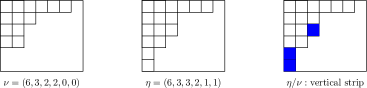
Figure 1. Young diagrams of partitions $\eta,\nu$

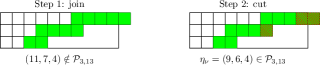
Figure 2. Associated parition $\eta_{\nu}$ by a join-and-cut operation

Lemma 3.16.

Let $1\leq p\leq m$ and $v,w\in W^{P}$. Denote $\nu:=\varphi_{m}(v)$ and $\eta:=\varphi_{m}(w)$. Then $w\in S_{m,p}(v)$ if and only if both of the following hold:

$$\mbox{(i)}\,\,|\eta|=|\nu|+p;\qquad\mbox{(ii)}\,\,\eta_{j}-\nu_{j}\in\{0,1\}\quad\mbox{ for all }1\leq j\leq m.$$

Furthermore when this holds, we have $\mu_{w,v,m}=\eta_{\nu}$.

Proof.

We assume $w\in S_{m,p}(v)$ first. Write $w=v\zeta_{1}\cdots\zeta_{d}$ where $\zeta_{1},\cdots,\zeta_{d}$ are pairwise disjoint cycles. Since $v,w\in W^{P}$, it follows that $v\zeta_{1}\cdots\zeta_{k}\in W^{P}$ for all $1\leq k\leq d$. Denote $p_{k}:=\ell(v\zeta_{1}\cdots\zeta_{k})-\ell(v\zeta_{1}\cdots\zeta_{k-1})$. Then $v\zeta_{1}\cdots\zeta_{k}\in S_{m,p_{k}}(v\zeta_{1}\cdots\zeta_{s-1})$ follows from the definition. In particular, write $\zeta_{1}=(ri_{p_{1}}\cdots i_{2}i_{1})$, then we have

$$(1)\,\,i_{1},\cdots,i_{p_{1}}\leq m<r;\qquad(2)\,\,v(r)>v(i_{1})>\cdots>v(i_{p_{1}}).$$

Claim F: Denote $i_{0}:=r$. We have

$$(a)[i_{p_{1}},\cdots,i_{2},i_{1}]=[i_{1}-p+1,\cdots,i_{1}-1,i_{1}];\quad(b)\,\,v(i_{j})=v(i_{j+1})+1,0\leq j\leq p_{1}-1.$$

Assuming the above claim first, we write $\varphi_{m}(v\zeta_{1})=(\eta^{(1)}_{1},\cdots,\eta^{(1)}_{m})=:\eta^{(1)}$. For any $1\leq s\leq m$ distinct from those $m+1-i_{j}$, we have

$$\eta^{(1)}_{s}=v\zeta_{1}(m+1-s)-(m+1-s)=v(m+1-s)-(m+1-s)=\eta_{s}.$$

By Claim F (b), we have

$$\eta_{m+1-i_{j}}^{(1)}=v\zeta_{1}(i_{j})-i_{j}=v(i_{j-1})-i_{j}=v(i_{j})+1-i_{j}=\eta_{m+1-i_{j}}+1.$$

Together with Claim F (a), we obtain

$$(**):\quad\eta^{(1)}=(\nu_{1},\cdots,\nu_{m-i_{1}},\nu_{m-i_{1}+1}+1,\cdots,\nu_{m-i_{1}+p_{1}}+1,\nu_{m-i_{1}+p_{1}+2},\cdots,\nu_{m}),$$

where $p_{1}\leq i_{1}\leq m$. Thus if $d=1$, then we are done.

Now we assume $d\geq 2$. Write $\zeta_{2}=(r^{\prime}i_{p_{2}}^{\prime}\cdots i_{2}^{\prime}i_{1}^{\prime})$. Since $\zeta_{1},\zeta_{2}$ are disjoint cycles, $m+1-i_{j}\not\in\{m+1-i_{1}^{\prime},\cdots,m+1-i^{\prime}_{p_{2}}\}$. Write $\varphi_{m}(v\zeta_{1}\zeta_{2})=\eta^{(2)}=(\eta_{1}^{(2)},\cdots,\eta^{(2)}_{m})$. Then $\eta_{s}^{(2)}=\eta^{(1)}_{s}$ whenever $s\in\{m+1-i_{1},\cdots,m+1-i_{p_{1}}\}$. Using the same arguments as above, we conclude $\eta_{s}^{(2)}-\eta_{s}^{(1)}\in\{0,1\}$ for all $s\in\{1,\cdots,m\}\setminus\{m+1-i_{1},\cdots,m+1-i_{p_{1}}\}$. Thus we have $\eta_{s}^{(2)}-\nu_{s}\in\{0,1\}$ for all $1\leq s\leq m$. Hence, both (i) and (ii) hold by induction on $k$.

As a direct consequence of the above arguments, we observe that $1\leq a\leq m$ occurs in some cycle $\zeta_{s}$ if and only if $\eta_{m+1-a}-\nu_{m+1-a}=1$. Hence, $[v(m+1-j_{1}),v(m+1-j_{2}),\cdots,,v(m+1-j_{m-p})]$ is the decreasing sequence obtained by sorting $\{v(1),\cdots,v(m)\}\setminus\{v(a)~{}|~{}a\mbox{ occurs in }\zeta_{s}\mbox{ for some }$ $1\leq s\leq d\}$. Hence, the partition $\mu_{w,v,m}=(\mu_{1},\cdots,\mu_{m-p})$ in $\mathcal{P}_{m-p,n+1}$ coincides with $\eta_{\nu}$, by noting

$$\mu_{i}=v(m+1-j_{i})-(m-p+1-i)=v(m+1-j_{i})-(m+1-j_{i})+p+i-j_{i}=\nu_{j_{i}}+p+i-j_{i}.$$

On the other hand, we assume the hypotheses (i) and (ii) both hold now. If $\varphi_{m}(w)=\eta$ is given by $(**)$, we define $i_{j}:=i_{1}-j+1$ for every $1\leq j\leq p_{1}$ and define $r$ to be the element satisfying $v(r)=v(i_{1})+1$. It is easy to check $r>m$. Consequently, we have $w=v(ri_{p_{1}}\cdots i_{2}i_{1})\in S_{m,p_{1}}(v)$ with $p_{1}=\ell(w)-\ell(v)=p$. In general, there are $d$ nests of consecutive $1$, for which we can construct pairwise disjoint cycles $\zeta_{1},\cdots,\zeta_{d}$ by induction, such that $w=v\zeta_{1}\cdots\zeta_{d}\in S_{m,p}(v)$.

It remains to show Claim F. It follows from $v\in W^{P}$ and properties (1), (2) that $m\geq i_{1}>i_{2}>\cdots>i_{p_{1}}$. If (a) did not hold, then $i_{j}>i_{j+1}+1$ for some $1\leq j\leq p_{1}-1$, and we would deduce a contradiction:

$$v(i_{j})=v\zeta_{1}(i_{j+1})<v\zeta_{1}(i_{j+1}+1)=v(i_{j+1}+1)<v(i_{j}).$$

Hence, (a) holds. If (b) did not hold, then $v(i_{j})>v(i_{j+1})+1$ for some $0\leq j\leq p_{1}-1$. If $j>0$, then $i_{j+1}+1=i_{j}$ by Claim F (a), and consequently $v(r)>v(i_{j+1})+1=v(a)$ for some $m+1<a<r$. In this case, we deduce a contradiction:

$$v(a)=v\zeta_{1}(a)<v\zeta_{1}(r)=v(i_{p_{1}})\leq v(i_{j+1})=v(a)-1.$$

If $j=0$, then $v(r)>v(i_{1})+1=v(b)$ for some $b<r$. If $b>m$, then we would have $v(b)=v\zeta_{1}(b)<v\zeta_{1}(r)=v(i_{p_{1}})\leq v(i_{1})=v(b)-1$. If $b\leq m$, then $b>i_{1}$ and consequently we have $v(r)=v\zeta_{1}(i_{1})<v\zeta_{1}(b)=v(b)<v(r)$. Either cases deduces a contradiction again. ∎

Using the above lemma, we can simplify Theorem 3.10 for the special case of complex Grassmannians, and therefore obtain the following. The proof is essentially the same as Corollary 3.3 of [CFon]. There is only one quantum variable in $QH^{*}_{T}(Gr(m,n+1))$, which we simply denote as $q$.

Theorem 3.17 (Equivariant quantum Pieri rule for complex Grassmannians).

Let $1\leq p\leq m$ and $\nu=(\nu_{1},\cdots,\nu_{m})\in\mathcal{P}_{m,n+1}$. In $QH^{*}_{T}(Gr(m,n+1))$, we have

$$\sigma^{1^{p}}\star\sigma^{\nu}=\sum_{r=0}^{p}\sum_{\eta}\xi^{m-r,p-r}(\eta_{\nu})\sigma^{\eta}+\sum_{r=0}^{p-1}\sum_{\kappa}\xi^{m-1-r,p-1-r}(\kappa^{\prime}_{\nu^{\prime}})\sigma^{\kappa}q,$$

where the second sum is over those $\eta=(\eta_{1},\cdots,\eta_{m})\in\mathcal{P}_{m,n+1}$ satisfying $|\eta|=|\nu|+r$ and $\eta_{i}-\nu_{i}\in\{0,1\}$ for all $1\leq i\leq m$; the $q$-terms occur only if $\nu_{1}=n+1-m$, and when this holds, the last sum is over those $\kappa=(\kappa_{1},\cdots,\kappa_{m-1},0)\in\mathcal{P}_{m,n+1}$ such that $\kappa^{\prime}:=(\kappa_{1}+1,\cdots,\kappa_{m-1}+1)$ and $\nu^{\prime}:=(\nu_{2},\cdots,\nu_{m})$ satisfy $|\kappa^{\prime}|=|\nu^{\prime}|+r$ and $\kappa_{i}+1-\nu_{i+1}\in\{0,1\}$ for all $1\leq i\leq m-1$.

Proof.

Denote $v=\varphi_{m}^{-1}(\nu)$. Using the same notations as in Theorem 3.10, we have $k=1$, and hence $\mbox{Pie}_{1,p}\subset\{(0),(1)\}$. By Theorem 3.10, we have

$$\sigma^{1^{p}}\star\sigma^{\nu}=\sum_{j=0}^{p}\sum_{w\in S_{m,j}}\xi^{m-j,p-j}(\mu_{w,v,m})\sigma^{w}+\epsilon\sum_{j=0}^{p-1}\sum_{w}\xi^{m-1-j,p-1-j}(\mu_{w\cdot\phi_{(1)},v\cdot\tau_{(1)},m-1})\sigma^{w}q,$$

where $\epsilon=1$ if $\ell(v\cdot\tau_{(1)})=\ell(v)-\ell(\tau_{(1)})$, or $0$ otherwise; the last sum is over those $w\in\mbox{Pie}((1))$ satisfying $w\cdot\phi_{(1)}\in S_{m-1,j}(v\cdot\tau_{(1)})$.

The classical part of the formula to prove is referred to as the equivariant Pieri rule. It follows from the canonical injective morphism $H_{T}^{*}(Gr(m,n+1))\hookrightarrow H^{*}_{T}(F\ell_{n+1})$ that $\xi^{m-j,p-j}(\mu_{w,v,m})\neq 0$ only if $w\in W^{P}$. Hence, the equivariant Pieri rule follows directly from Lemma 3.16.

When $\mathbf{d}=(1)$, we have $\tau_{\mathbf{d}}=s_{m}s_{m+1}\cdots s_{n}$ and $\phi_{\mathbf{d}}=s_{1}s_{2}\cdots s_{m-1}$. Note $v(m)=\max\{v(1),\cdots,v(m)\}$ and $v(n+1)=\max\{v(m+1),\cdots,v(n+1)\}$. As a consequence, the following are all equivalent:

$$\mbox{i) }\ell(v\cdot\tau_{(1)})=\ell(v)-\ell(\tau_{(1)});\mbox{ ii) }v\tau_{\mathbf{d}}(\alpha_{n})\in R^{+};\mbox{ iii) }v(m)>v(n+1);\mbox{ iv) }v(m)=n+1.$$

Hence, we have $\epsilon=1$ if and only if $\nu_{1}=v(m)-m=n+1-m$. Furthermore when this holds, $v\cdot\tau_{(1)}$ is a Grassmannian permutation for $Gr(m-1,n+1)$, which corresponds to the partition $\varphi_{m-1}(v\cdot\tau_{(1)})=(\nu_{2},\cdots,\nu_{m-1})=:\nu^{\prime}$ in $\mathcal{P}_{m-1,n+1}$ (by noting $v\tau_{\mathbf{d}}(j)=v(j)$ for $1\leq j\leq m-1$).

Write $\varphi_{m}(w)=(\kappa_{1},\cdots,\kappa_{m})=:\kappa$. Then the following are equivalent:

$$(1)\,\,w\in\mbox{Pie}((1));\quad(2)\,\,\ell(w\cdot\phi_{(1)})=\ell(w)+\ell(\phi_{(1)});\quad(3)\kappa_{m}=0.$$

It follows that $w\cdot\phi_{(1)}$ is a Grassmannian permutation for $Gr(m-1,n+1)$, which corresponds to the partition $\varphi_{m-1}(w\cdot\phi_{(1)})=(\kappa_{1}+1,\cdots,\kappa_{m-1}+1)=:\kappa^{\prime}$.

Hence, the $q$-part also becomes a direct consequence of Lemma 3.16. ∎

Remark 3.18.

The non-equivariant quantum Pieri rule [Bertram] can be obtained by using Proposition 11.10 of [LaSh-GoverPaffineGr] and the Pieri-type formula of $H_{*}(\Omega SU(n+1))$ in [LLMS]. It will be very interesting to generalize this approach to the equivariant quantum cohomology of complex (or more generally, cominuscule) Grassmannians.

Example 3.19.

Among the product $\sigma^{(1,1,0)}\star\sigma^{(4,2,1)}$ in $H^{*}_{T}(Gr(3,7))$, two terms $q^{0}\sigma^{\eta}$ and $q^{1}\sigma^{\kappa}$ can be read off from the following figure:

By calculating the remaining terms in the product by Theorem 3.17, we have

$$\sigma^{(1,1,0)}\star\sigma^{(4,2,1)}$$

$$= (\alpha_{1}+\alpha_{2}+\alpha_{3})(\alpha_{1}+\cdots+\alpha_{6})\sigma^{(4,2,1)}+(\alpha_{1}+2\alpha_{2}+2\alpha_{3}+\alpha_{4}+\alpha_{5}+\alpha_{6})\sigma^{(4,2,2)}$$

$$+(\alpha_{1}+\cdots+\alpha_{6})\sigma^{(4,3,1)}+\sigma^{(4,3,2)}+q\sigma^{(1,1,0)}+q\sigma^{(2,0,0)}+(\alpha_{1}+\alpha_{2}+\alpha_{3})q\sigma^{(1,0,0)}$$

Corollary 3.20.

In $QH^{*}_{T}(Gr(m,n+1))$, we have

$$\sigma^{1^{p}}\star\sigma^{(n+1-m,0,\cdots,0)} =\sigma^{1^{p}}\circ\sigma^{(n+1-m,0,\cdots,0)},\quad\mbox{for }1\leq p<m;$$

$$\sigma^{1^{m}}\star\sigma^{(n+1-m,0,\cdots,0)} =(\alpha_{1}+\cdots+\alpha_{n})\sigma^{(n+1-m,1,\cdots,1)}+q.$$

Proof.

Let $1\leq p\leq m$ and $\nu=(n+1-m,0,\cdots,0)$. It follows directly from Theorem 3.17 that all possible partitions are given by $\eta^{(r)}:=(n+1-m,1,\cdots,1,0,\cdots,0)$ where $|\eta^{(r)}|=n+1-m+r$, $0\leq r\leq m-1$; and the $q$-terms occur only if there exists $\kappa$ satisfying $p-1\geq r=|\kappa^{\prime}|=m-1+|\kappa|\geq m-1$. Hence, if $p<m$, then $\sigma^{1^{p}}\star\sigma^{(n+1-m,0,\cdots,0)}$ involves no $q$-terms. If $p=m$, then $|\kappa|=0$, namely $(0,\cdots,0)$ is the only partition satisfying the required properties. Hence,

$$\sigma^{1^{m}}\star\sigma^{\nu}=\sum_{r=0}^{m-1}\xi^{m-r,m-r}(\eta^{(r)}_{\nu})\sigma^{\eta}+\xi^{m-1-(m-1),m-1-(m-1)}\big{(}(1,\cdots,1)_{(0,\cdots,0)}\big{)}\sigma^{\scriptsize\mbox{id}}q,$$

in which we note $\xi^{0,0}\big{(}(1,\cdots,1)_{(0,\cdots,0)}\big{)}=1$. By definition, we have $\eta^{(r)}_{\nu}=(n+1-m+r,0,\cdots,0)\in\mathcal{P}_{m-r,n+1}$. Hence, $\xi^{m-r,m-r}(\eta^{(r)}_{\nu})=0$ unless $r=m-1$. Furthermore when $r=m-1$, we have

$$\xi^{m-r,m-r}(\eta^{(r)}_{\nu})=\xi^{1,1}((n,0,\cdots,0))=s_{n}s_{n-1}\cdots s_{2}(\alpha_{1})=\alpha_{1}+\cdots+\alpha_{n}.$$

Hence, the statement follows. ∎

Appendix: Equivariant quantum Giambelli formula for complex Grassmannians

We expect out equivariant quantum Pieri rule to have further applications in the equivariant quantum Schubert calculus. To illustrate our expectation, we will reprove [Mihalcea-EQGiambelli, Theorem 3.22]. That is, we will study $QH^{*}_{T}(Gr(m,n+1))$, giving alternative proofs of the ring presentation and the equivariant quantum Giambelli formula. In our approach, we use the equivariant quantum Pieri rule as in Theorem 3.17, together with the equivariant Giambelli formula [Mihalcea-EQGiambelli, LaRaSa]. This is completely similar to the one given by Buch [Buch-Grassmannian] for the non-equivariant quantum cohomology $QH^{*}(Gr(m,n+1))$.

We follow [Mihalcea-EQGiambelli] for the next facts on equivariant cohomology $H^{*}_{T}(Gr(m,n+1))$. Treat $S=\mathbb{Z}[\alpha_{1},\cdots,\alpha_{n}]$ as a subring of $\mathbb{Z}[\mathbf{t}]=\mathbb{Q}[t_{1},\cdots,t_{n+1}]$ via

$$\alpha_{i}\mapsto t_{n+2-i}-t_{n+1-i},\quad i=1,\cdots,n.$$

By convention, we denote $t_{i}=0$ if $i\leq 0$ or $i\geq n+2$. Let $e_{i}=e_{i}(x_{1},\cdots,x_{m};\mathbf{t}),i=1,\cdots,m$ (resp. $h_{j}=h_{j}(x_{1},\cdots,x_{m};\mathbf{t}),j=1,\cdots,\cdots,{n+1-m}$) denote the elementary (resp. complete) homogeneous factorial Schur functions. By convention, we denote $e_{0}=h_{0}=1$, $e_{i}=0$ if $i<0$ or $i>m$, and $h_{j}=0$ if $j<0$ or $j>n+1-m$. Define $\tau^{s}$ inductively by $\tau^{0}e_{p}:=e_{p}\,\,\,\mbox{ and }\,\,\,\tau^{s}e_{p}:=\tau^{s-1}e_{p}+(t_{s}-t_{m-p+s+1})\tau^{s-1}e_{p-1}.$ Denote by $\lambda^{T}:=(\lambda_{1}^{T},\cdots,\lambda_{n+1-m}^{T})\in\mathcal{P}_{n+1-m,n+1}$ the transpose of a given partition $\lambda\in\mathcal{P}_{m,n+1}$. Let $H_{k}:=\det\big{(}\tau^{j-1}e_{1+j-i}\big{)}_{1\leq i,j\leq k}.$ We will need the next lemma, which follows directly from equation (2.10) of [Mihalcea-EQGiambelli]

Lemma 3.21.

For any $M\in\mathbb{Z}^{+}$, in $H_{T}^{*}(Gr(m,n+1))$, we have

$$\sum_{p=0}^{m}(-1)^{p}\sigma^{1^{p}}\circ\tau^{1-M}H_{M-p}=0$$

with $\tau^{0}H_{j}:=H_{j}$ and $\tau^{-s}H_{j}:=\tau^{1-s}H_{j}+(t_{j+m-s}-t_{1-s})\tau^{1-s}H_{j-1}.$

Theorem 3.22 (Equivariant quantum Giambelli formula; Theorem 4.2 of [Mihalcea-EQGiambelli]).

There is a canonical isomorphism of $S[q]$-algebras,

$$S[q][e_{1},\cdots,e_{m}]/\langle H_{n-m+2},\cdots,H_{n},H_{n+1}+(-1)^{m}q\rangle\longrightarrow QH^{*}_{T}(Gr(m,n+1)),$$

defined by $e_{p}\mapsto\sigma^{1^{p}}$. Under this isomorphism, $\sigma^{r}=H_{r}$ for $r\leq n+1-m$, and

$$\sigma^{\lambda}=\det\big{(}\tau^{j-1}e_{\lambda_{i}^{T}+j-i}\big{)}_{1\leq i,j\leq n+1-m}.$$

Proof.

It is sufficient (1) to calculate $H_{k}$ and $\det\big{(}\tau^{j-1}e_{\lambda_{i}^{T}+j-i}\big{)}$ with respect to the equivariant quantum product and (2) to subtract the quantum corrections, by an equivariant quantum extension of [FuPa, Proposition 11] (or [SiTi, Proposition 2.2]). The known ring presentation of $H_{T}^{*}(Gr(m,n+1))$ is read off from the first half of the statement by evaluating $q=0$, and the known equivariant Giambelli formula is exactly of the same form as in the second half. Thus for any $\lambda\in\mathcal{P}_{m,n+1}$, we have

$$\det\big{(}\tau^{j-1}e_{\lambda_{i}^{T}+j-i}\big{)}_{1\leq i,j\leq n+1-m}=\sigma^{\lambda}+q\cdot g_{\lambda}\,\,\mbox{ in }QH^{*}_{T}(Gr(m,n+1)),$$

for some element $g_{\lambda}\in QH^{*}_{T}(Gr(m,n+1))$. The determinant $\det\big{(}\tau^{j-1}e_{\lambda_{i}^{T}+j-i}\big{)}$ in $QH^{*}_{T}(Gr(m,n+1))\otimes_{S}\mathbb{Z}[\mathbf{t}]$ is a summation of the form

$$f(\mathbf{t})\sigma^{1^{i_{1}}}\star\sigma^{1^{i_{2}}}\star\cdots\star\sigma^{1^{i_{n+1-m}}}.$$

By Theorem 3.17 and induction, the expansion of $\sigma^{1^{i_{1}}}\star\sigma^{1^{i_{2}}}\star\cdots\star\sigma^{1^{i_{j}}}$ involves no $q$-terms, and all Schubert classes in the expansion are of the form $\sigma^{\mu}$, $\mu=(\mu_{1},\cdots,\mu_{m})$ with $\mu_{1}\leq j$. Hence, $g_{\lambda}=0$. That is, the second part of the statement holds, by noting that the determinant lies in $QH^{*}_{T}(Gr(m,n+1))$. In particular, we have $H_{r}=\sigma^{r}$ in $QH^{*}_{T}(Gr(m,n+1))$, for $r=0,1,\dots,n-m+1$.

Clearly, $\tau^{j-1}e_{1+j-i}$ is zero if $1+j<i$, or of degree $1+j-i$ otherwise. Hence, $\deg H_{r}=r$. Since $\deg q=\langle c_{1}(T_{Gr(m,n+1)}),\sigma_{s_{k}}\rangle=n+1$, it follows that no $q$-term is involved in the expansion of $H_{r}$ in $QH^{*}_{T}(Gr(m,n+1))$, whenever $r<n+1$.

In $H^{*}_{T}(Gr(m,n+1))$ it follows from Lemma 3.21 with respect to $M=n+1$ that

$$H_{n+1}=(-1)^{m-1}e_{m}H_{n+1-m}+\sum_{i=0}^{n}f_{i}(\mathbf{t})H_{i}+\sum_{j=0}^{n-m}g_{m,j}(\mathbf{t})e_{m}H_{j}+\sum_{p=1}^{m-1}\sum_{r=0}^{n-p}g_{p,j}(\mathbf{t})e_{p}H_{r}$$

for some $f_{i},g_{m,j},g_{p,r}\in\mathbb{Z}[\mathbf{t}]$. Now we compute the $q$-terms in the expansion of the right-hand side as multiplications in $QH^{*}_{T}(Gr(m,n+1))\otimes_{S}\mathbb{Z}[\mathbf{t}]$. With respect to the equivariant quantum multiplications, we have shown $H_{r}=0$ if $n-m+2\leq r\leq n$, and $H_{r}=\sigma^{r}$ if $0\leq r\leq n-m+1$. Hence, it follows from Theorem 3.17 (resp. Corollary 3.20) that $\sum_{j=0}^{n-m}g_{m,j}(\mathbf{t})\sigma^{1^{m}}\star\sigma^{p}$ (resp. $\sum_{p=1}^{m-1}\sum_{r=0}^{n-p}g_{p,j}(\mathbf{t})\sigma^{1^{p}}H_{r}$) involves no $q$-terms. Hence, the only $q$-term in the expansion of $H_{n+1}$ comes from

$$(-1)^{m-1}\sigma^{1^{m}}\sigma^{n-m+1}=(-1)^{m-1}((\alpha_{1}+\cdots+\alpha_{n})\sigma^{(n+1-m,1,\cdots,1)}+q),$$

by Corollary 3.20 again. Hence, $H_{n+1}=(-1)^{m-1}q$ in $QH^{*}_{T}(Gr(m,n+1))$. ∎