An examination of proton charge radius extractions from e-p scattering data

Abstract

A detailed examination of issues associated with proton radius extractions from elastic electron-proton scattering experiments is presented. Sources of systematic uncertainty and model dependence in the extractions are discussed, with an emphasis on how these may impact the proton charge and magnetic radii. A comparison of recent Mainz data to previous world data is presented, highlighting the difference in treatment of systematic uncertainties as well as tension between different data sets. We find several issues that suggest that larger uncertainties than previously quoted may be appropriate, but do not find any corrections which would resolve the proton radius puzzle.

I Introduction

Five years after the initial extraction of the proton radius from muonic hydrogen Pohl et al. (2010), the “proton radius puzzle” persists. Measurements based on muonic hydrogen transitions Antognini et al. (2013) and those based on electron transitions Mohr et al. (2012) or electron scattering measurements Zhan et al. (2011); Sick (2012); Bernauer et al. (2014) disagree at the 7$\sigma$ level, with muonic hydrogen results yielding a radius near 0.84 fm and electron-based measurements yielding $r_{E}\approx 0.88$fm, as summarized in Fig. 1. In light of this, a careful examination of the details of these extractions is clearly warranted. Here, we discuss several issues relevant to determining the proton radius from electron scattering data.

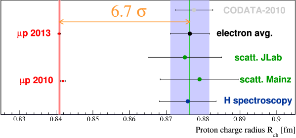
Figure 1: Extractions of the proton charge radius from muonic hydrogen measurements Pohl et al. (2010); Antognini et al. (2013), hydrogen spectroscopy Mohr et al. (2012), electron scattering measurements at Mainz Bernauer et al. (2014); unc , and a global analysis of earlier world data Zhan et al. (2011). The direct average shown is compared to the CODATA-2010 evaluation Mohr et al. (2012). Figure courtesy of Randolf Pohl.

In examining extractions from electron scattering data, we examine the Mainz data Bernauer et al. (2014) and global analyses Zhan et al. (2011); Sick (2012) of world data (excluding Mainz) separately. This is done because the Mainz data presents the uncertainties in the data in a significantly different way from most other experiments, making it difficult to perform a meaningful combined analysis. It is also beneficial to perform independent analyses to examine consistency between the Mainz data and other measurements at the cross sections level, which can be overlooked in a combined analysis. We also discuss some preliminary results from a detailed examination of both Mainz and world data Lee et al. (2015). There are several issues that suggest that larger uncertainties than quoted in previous works are warranted. While none of these appear likely to resolve to the discrepancy with muonic hydrogen measurements, some issues remain which deserve more detailed examination.

II General issues in the extraction of the radii

One obtains the charge and magnetic form factors, $G_{E}(Q^{2})$ and $G_{M}(Q^{2})$, from unpolarized cross section measurements by performing a Rosenbluth separation Rosenbluth (1950) which uses the angle-dependence at fixed $Q^{2}$ to separate the charge and magnetic contributions. The cross section at fixed $Q^{2}$ is proportional to the ’reduced’ cross section $\sigma_{R}=\tau G_{M}^{2}+\varepsilon G_{E}^{2}$, where $\tau=Q^{2}/(4M_{p}^{2})$ and $\varepsilon^{-1}=[1+2(1+\tau)\tan^{2}(\theta/2)]$. At low $Q^{2}$, the magnetic contribution is strongly suppressed except for very small $\varepsilon$ values, corresponding to large scattering angle. Because of the difficulties in making very large angle scattering measurements at low $Q^{2}$, a significant extrapolation to $\varepsilon=0$ is required and even sub-percent uncertainties on the cross sections can yield significant uncertainties on small contribution from $G_{M}(Q^{2})$.

Because one often combines data from many experiments, each of which has an uncertainty in its normalization uncertainty, the normalizations factors of the limited number of large-angle data sets have a great impact on the extraction of $G_{M}$. If these normalization factors are allowed to vary in the fit, which is the most common approach, then a small shift in normalization between large and small angle data sets can yield a significant shift of strength between $G_{E}$ and $G_{M}$ over a range in $Q^{2}$ values. Polarization observables are sensitive to the ratio $G_{E}/G_{M}$ Perdrisat et al. (2007); Arrington et al. (2007a) and can thus provide not only direct information on the form factors, but also improve the determination of the relative normalization of different measurements. Of particular interest are data sets at low $Q^{2}$ values Ron et al. (2007); Crawford et al. (2007); Zhan et al. (2011); Ron et al. (2011) which provide improved extractions of $G_{M}$ and additional constraints on the experimental normalizations.

Extraction of the charge radius from electron scattering requires parameterizing the cross sections to obtain the slope of the form factor at $Q^{2}=0$. Many naive extractions use fit functions which do not provide sufficient flexibility to accurately describe the low-$Q^{2}$ data, and often do not attempt to estimate the uncertainty associated with the choice of functional form used to fit the data. For example, several early extractions were based on linear fits to low $Q^{2}$ data. Such fits will always give an underestimate of the radius, based on the observed positive curvature of the form factors at low $Q^{2}$. One would have to have extremely precise data at very low $Q^{2}$ for a linear fit to be sufficient Sick (2003); Kraus et al. (2014).

Simply increasing the number of parameters in a simple Taylor expansion or similar fit function provides greater flexibility. However, it also leads to increased uncertainty in the extracted radius as correlations between different parameters in the expansion allow the impact of variations in one term of the expansion to be balanced by changes in other terms. This yields a rapid increase in the extracted radius uncertainty as the number of parameters is increased. This may lead to a situation where there is no region in which there are enough parameters to accurately reproduce the data while still yielding an uncertainty small enough to provide a useful radius extraction Lee et al. (2015). Such analyses must find a balance between fit flexibility and radius uncertainty and, ideally, attempt to estimate the error made when truncating the fit function. All of the extractions that we will review in detail Zhan et al. (2011); Sick (2012); Bernauer et al. (2014) examine the model dependence associated with the functional form used to parameterize the data and include at least some estimate of the associated uncertainty.

The factor $\tau$ suppresses the magnetic contribution as $Q^{2}\to 0$, causing the uncertainties on $G_{M}(Q^{2})$ to increase rapidly as seen in Fig. 2. Because the radius extraction is sensitive to the low-$Q^{2}$ behavior of $G_{M}$ and the most precise data are at higher $Q^{2}$ values, it is particularly difficult to reliably extract the magnetic radius. In the analyses of world data Zhan et al. (2011); Sick (2012), the fits exclude high-$Q^{2}$ data to prevent these data from influencing the extraction of the slope. For the analysis of the Mainz data Bernauer et al. (2014), the data set extends to $Q^{2}\approx 1$ GeV², but the bulk of the data below $Q^{2}=0.5$ GeV² and a more flexible fit function is used to provide greater flexibility to fit cross section measurements at both low and high $Q^{2}$.

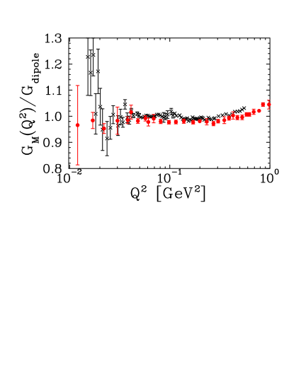
Figure 2: Extractions of $G_{M}$ and their uncertainties from direct Rosenbluth separations for the Mainz data Bernauer et al. (2014) (crosses) and from a global (pre-Mainz) analysis Arrington et al. (2007b) (circles).

Radiative corrections are another area requiring special attention. The largest contributions to the radiative corrections can be calculated in a model-independent way, although there are small variations between different prescriptions Mo and Tsai (1969); Maximon and Tjon (2000); Vanderhaeghen et al. (2000); Ent et al. (2001). Other terms, in particular the two-photon exchange (TPE) contributions Carlson and Vanderhaeghen (2007); Arrington et al. (2011), are model dependent as it is necessary to account for the possible hadronic states in between the two exchanged photons. The world data analyses Zhan et al. (2011); Sick (2012) include two-photon exchange corrections based on a calculation in a hadronic basis including only intermediate proton state Blunden et al. (2005), although estimates of excited states Kondratyuk et al. (2005); Kondratyuk and Blunden (2007) suggest that their contribution is very small at the relevant $Q^{2}$ values. The radiative correction uncertainties quoted by the experiments used in these global analyses were typically 1-1.5%, and are assumed to be sufficient after applying the calculate TPE corrections. We note that the data of Simon, et al. Simon et al. (1980, 1981) did not include any uncertainty for radiative corrections and thus tend to have an artificially enhanced impact on extractions of the form factors and radius. In the analysis of Ref. Zhan et al. (2011), and additional radiative correction uncertainty was applied to the Simon data.

The primary result from the Mainz experiment Bernauer et al. (2014) applies TPE corrections derived for a point target McKinley and Feshbach (1948) (the “Feshbach” correction). This correction is exact for $Q^{2}=0$ but has no $Q^{2}$ dependence. Because the radius is the $Q^{2}$ slope of the form factors at $Q^{2}=0$, it seems unlikely that a $Q^{2}$-independent correction will be sufficient. The model-dependent TPE calculations mentioned above agree with the Feshbach correction at $Q^{2}=0$, but as $Q^{2}$ increases they tend to decrease, going to zero before changing sign and growing in magnitude above $Q^{2}\approx 0.3$ GeV². There are several TPE calculations meant to be appropriate at low $Q^{2}$ Blunden et al. (2005); Borisyuk and Kobushkin (2006, 2008); Kondratyuk et al. (2005); Borisyuk and Kobushkin (2007, 2012, 2013), and they are all in good agreement at low $Q^{2}$ as shown in Ref. Arrington (2013). Very recently, this change of sign relative to the $Q^{2}=0$ limit was confirmed by comparisons of electron-proton and positron-proton scattering for $Q^{2}\approx 1$ and 1.5 GeV² Adikaram et al. (2015); Rachek et al. (2015). This supports the idea that the $Q^{2}=0$ calculation is not appropriate and a more complete TPE correction is required.

The question of TPE corrections in the Mainz data was first examined in Refs. Arrington (2011); Bernauer et al. (2011). Ref. Bernauer et al. (2011) shows a direct comparison of the extracted value of $\mu_{p}G_{E}/G_{M}$ with and without TPE corrections from Ref. Borisyuk and Kobushkin (2007), which are expected to be valid up to $Q^{2}\approx 0.1$ GeV². As noted in Bernauer et al. (2011), the correction on $\mu_{p}G_{E}/G_{M}$ is relatively small, below 1%. However, this correction is larger than the linear sum of the statistical, systematic, and model uncertainties. It is, therefore, a critical correction for an extraction aimed at such high precision, and clearly necessary for a precise extraction of the charge and magnetic radii. Ref. Bernauer et al. (2014) does not include any uncertainty associated with TPE corrections, but does include an extraction of the radius after applying hadronic corrections with the proton intermediate state Blunden et al. (2005). The change in the charge radius is 0.004 fm, roughly 1/3 of the total uncertainty unc , while the magnetic radius changes by 0.022 fm, more than the total quoted uncertainty.

III Examination of the Mainz analysis

As noted earlier, the extraction of the uncertainties as well as the breakdown of different types of uncertainties in the recent Mainz data set is significantly different from other experiments. We describe the approach used in Ref. Bernauer et al. (2014), and then discuss potential implications on the uncertainties of the extracted radii in the Mainz analysis, as well as independent fits to the Mainz cross section data.

III.1 Uncorrelated systematic uncertainty

The uncorrelated systematic uncertainties were determined by performing a fit to the full data set using only the pure counting statistics for uncertainties. The difference between the data and fit for each subset (each independent energy-spectrometer combination) was examined, and a scaling factor was determined for each data set which, when applied as a scale factor enhancement to the uncertainties from the counting statistics on every data point, yielded a scatter that was approximately consistent with the enhanced statistical uncertainty. The goal is to provide a reduced $\chi^{2}$ value closer to unity, with $\chi^{2}_{\nu}\approx 1.14$ for the final Mainz fit to the cross sections with the scaling factors applied. This procedure yields the minimal uncertainty necessary to account for the non-statistical scatter of the data, but is insensitive to any sources of error which may be correlated with the kinematics or operating conditions of the experiment, e.g. beam energy or spectrometer angle offsets, approximations in the radiative correction procedures, or subtraction of target cell wall contributions. In fact, because the final reduced chi-squared is still above one, the final uncorrelated systematic uncertainty is somewhat below the minimum necessary to account for the observed scatter.

This rescaling procedure is relatively unusual; nearly all other experiment made direct estimates of uncertainties or upper limits for various sources of uncertainty which may be treated as uncorrelated in the fit. This uncorrelated systematic is determined and added in quadrature to the statistical uncertainty. If we convert the Mainz scaling factors to independent systematic uncertainties using this standard approach, they correspond to uncertainties that average 0.25%, but vary from 0.02% to 2% with the smallest systematic uncertainties generally being applied to the data with smallest statistical uncertainties.

III.2 Correlated systematic uncertainty

Most experiments provide relatively small data sets, typically tens of cross section measurements covering a range of $Q^{2}$ and $\varepsilon$ values. For such data sets, correlated errors, e.g. associated with kinematic-dependent corrections, can be well represented by applying an additional uncorrelated uncertainty to each point. A modest 0.5% contribution to the uncertainty on each cross section provides flexibility to cover an arbitrary correlated uncertainty at the few tenths of a percent level. For the Mainz measurement there are 1422 cross sections, 10–50 times more than most experiments, so any limited kinematic region will have many more data points, reducing the impact of the uncorrelated uncertainty by the square root of the number of points. Thus, trying to represent small correlated effects as uncorrelated uncertainties would require much larger contributions.

This effect is made worse by the fact that of the 1422 data points, there are only 638 independent kinematic settings. In several cases, multiple repeated measurements were taken at the same kinematic setting, one after the other. For the given procedure - inflating the counting statistics by a scaling factor intended to yield a reasonable chi-squared for each data set - it doesn’t matter that there are multiple repeated measurements in the data set. However, using the more conventional approach of applying a fixed systematic uncertainty to each point, a set of $N$ repeated measurements would artificially reduce the impact of the systematic uncertainty by a factor of $\sqrt{N}$ for this kinematic setting. If the data are rebinned into their 638 independent points and a systematic applied that yields a reduced chi-squared value near unity, the uncertainties tend to increase more where the scaled uncertainties were very small, i.e. the very high statistics points or the kinematics with small scaling factors. This ends up increasing the low $Q^{2}$ data uncertainties more and yields a larger uncertainty on the extracted radius Lee et al. (2015).

Because of the limitations of including only uncorrelated systematic uncertainties on such a large data set, the A1 collaboration treated correlated systematic uncertainties independently. They separated the full data set into 18 subsets, each corresponding to a single spectrometer and fixed beam energy. They then simultaneously applied a correction factor, proportional to the scattering angle, to all points with each of these 18 subgroups and refit the data. The correction varied from 0% at the smallest angle to a setting-dependent maximum value at the largest angle for each setting. The size of this maximum correction, the parameter “$a$” from Ref. Bernauer et al. (2014), is shown for all 18 spectrometer/energy combinations in Fig. 3, with most settings having a value between 0.1% and 0.25%. In addition, that there is also a separate correlated systematic which accounts for variation of the cross section with the elastic tail cut, which is evaluated separately and then combined with correlated systematic mentioned above. As this is the smaller contribution, we focus here on the correction that is taken to be linear in $\theta$.

Note the in the supplemental material of Ref. Bernauer et al. (2014), the systematic correction does not go to zero for the smallest scattering angle of each subset, but goes to zero at $\theta=0$. If the normalization factors of the data subgroups are allowed to vary, the two procedures are equivalent. However, if the normalizations are not allowed to vary, applying the corrections factors as published will yield a much larger correlated error.

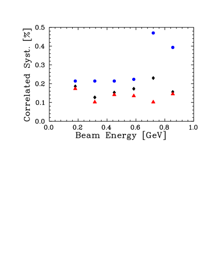
Figure 3: Size of the correlated systematic parameter $a$ for Spectrometer A (diamond), B (triangle), and C (circle) for each beam energy setting of Ref. Bernauer et al. (2014).

III.3 Normalization uncertainty

The combination of the uncorrelated and correlated uncertainties applied to the Mainz data are extremely small compared to other measurements and, by themselves, represent an incomplete estimate of the experimental uncertainty. The data are broken up into 34 subgroups, each of which has an independent, unconstrained normalization factor. Thus, the uncorrelated and correlated systematic uncertainties described above need only account for the variation of any corrections over the kinematics of the individual subgroups which consist of between 18 and 68 independent kinematics each (treating multiple runs at identical kinematics as single points), as the overall normalization factor will account for any average correction. Note, however, that there are 34 different normalization subgroups while the correlated systematic uncertainties are applied over the 18 independent beam energy-spectrometer combinations. It would seem more consistent for apply the correlated systematic over each of the 34 normalization subgroups, and the potential impact of this, as well as the choice of functional form for the correlated systematic, will be discussed in the following section.

III.4 Treatment of the uncertainties

Because the uncertainties of the measurement are separated into uncorrelated, correlated, and normalization uncertainties, a proper evaluation of the radius uncertainties must account for all of these. Fits which take the Mainz cross section data as quoted and do not allow the normalization factors to vary, e.g. as in Ref. Lorenz and Meißner (2014), will yield artificially small uncertainties in the radius extractions, as discussed in Ref. Lee et al. (2015).

In addition, questions have been raised about missing contributions to the uncertainties. No uncertainties associated with TPE corrections are included, and there are additional uncertainties associated with approximations made in radiative correction procedures. These are neglected in Bernauer et al. (2014), based on the assumption that these will be contained in the small correlated systematic uncertainties applied for other effects, but no argument is made to support these uncertainties being negligible compared to the typical 0.1-0.2% correlated systematic (Fig. 3). They also quote uncertainties on the knowledge of the beam energy and spectrometer scattering angles, but do not account for these in the cross section uncertainties. While the impact of these kinematic uncertainty on the cross sections is generally very small, the corrections for both energy and angle can be as large as 0.2%, mainly at low energy and small scattering angle, and are strongly kinematic dependent. Thus, it is not clear that they should be neglected in comparison to statistical uncertainties at the 0.2% level and correlated systematics which are as low as 0.1% for some settings.

It has also been noted Sick (2012) that the target cell wall contributions, subtracted from the data based on a calculated spectrum, don’t match the observed contribution. Based on the visible difference between the data and simulated spectrum in the region between the nuclear elastic and e-p elastic peaks (Fig. 8b of Ref. Bernauer et al. (2014)), it was estimated that this subtraction underestimates the cell contributions by 1.2% Sick (2012). This is a large effect, both compared to the quoted uncertainties of the measurement and to the size of the subtraction (below 4% for most settings Bernauer et al. (2011)). While this is the largest contribution to the correlated systematic uncertainty, it is still taken to be roughly 0.1-0.2% for nearly all settings. Any overall normalization error caused by an underestimate of the background subtraction will be removed in the fit, but with the subtraction varying from a few percent to nearly 10% for spectrometer B at forward angles Bernauer et al. (2011), it’s not clear that the kinematic variation over each of the data subsets can be constrained to be below the 0.1-0.2% level.

In addition to noting that the correlated systematic uncertainties applied are very small and may neglect important contributions, we also note that the impact of these uncertainties on the extracted form factors and radii are evaluated within a single model; a shift of the cross sections which is linear in $\theta$ over each of the 18 spectrometer-beam energy combinations. Taking the correction to scale with quantities other than $\theta$ can yield larger or smaller corrections, with an increase 50% or more in some models where the correction is not linear in angle Lee et al. (2015). Note that the procedure always yields a fixed correction between the smallest and largest angle settings of a given data subset, so it is only the form of the variation over this subset that is changed in these tests. The impact of the correlated systematic uncertainty is also significantly increased if it is taken as a correction to each data set with independent normalization, which seems a more consistent approach given the breakdown of uncertainties into uncorrelated, correlated, and normalization. Given the issues with the size of the correlated systematics noted above and the model dependence of converting these systematic effects into an uncertainty on the extracted radius, a conservative approach would appear to yield significantly larger radius uncertainties associated with the correlated systematics.

Note that the detailed comparisons in Ref. Lee et al. (2015) are performed for the rebinned version of the Mainz data. When examining the original analysis procedure Bernauer et al. (2014), the correlated systematic uncertainty on the extracted radii is more sensitive to both the functional form chosen to represent the correlated corrections and to the question of whether the correction is applied to each normalization subgroup or each beam-spectrometer combination.

IV Fitting with bounded $z$ expansion

As noted earlier, it is important that the fit function be flexible enough to adequately reproduce the data without being so flexible that it does not provide a meaningful constraint on the extracted radii. This is especially critical for the magnetic radius, where the precise high-$Q^{2}$ data can influence the fit more than the low-$Q^{2}$ data which are directly sensitive to the radius. Typically, a fit function is selected and the number of parameters is chosen to be as small as possible while still providing a reduced chi-squared that is close to the minimum value obtained for many parameters. In some cases, fit functions designed to help minimize the impact of the high-$Q^{2}$ data on the low-$Q^{2}$ fit are chosen, e.g. spline functions Bernauer et al. (2014) or continued fraction fits Sick (2003). However, it is still difficult to determine how many parameters are sufficient for a reliable fit. Figure 9.21 of Ref. Bernauer (2010) shows the extracted charge and magnetic radii vs. the number of parameters for a variety of different functional forms. For the charge radius, the extracted radii are relatively consistent for fits with 10-15 parameters, although there is a significant spread ($\approx 0.02$ fm) between the values using different fit functions. For more than 16 parameters, the spline fits yield much smaller radii, but this is presumably in the region where the uncertainties become very large and so the shift of the central value may not be outside of the fit uncertainty. For the magnetic radius, the situation is noticeably worse. There is a narrow window, 6-8 parameters, where the radii are relatively stable and then by 10 parameters the different functional forms yield radius values differing by nearly 0.2 fm. As noted in Ref. Sick and Trautmann (2014), some of this erratic behavior is associated with fits that have unphysical behavior, e.g. poles in the form factor and oscillatory behavior of the proton charge density, $\rho(r)$ at very large values of $r$.

One approach to this problem was presented in Refs. Sick (2012); Sick and Trautmann (2014), where a parameterization was chosen that constrains the large-$r$ behavior of the form factors. By including physical constraints on the behavior of the form factors, one can avoid the possibility that insufficiently flexible fit functions may yield a poor fit radius to better reproduce high-$Q^{2}$ data.

Another approach that can help address issues of over- or under-fitting data is the use of the bounded $z$ expansion Hill (2006). In this method, the form factors are parameterized as a polynomial in $z$ rather than $Q^{2}$, where

$$z(t,t_{\rm cut},t_{0})=\frac{\sqrt{t_{\rm cut}-t}-\sqrt{t_{\rm cut}-t_{0}}}{\sqrt{t_{\rm cut}-t}+\sqrt{t_{\rm cut}-t_{0}}}\,,$$ (1)

where $t_{\rm cut}=4m_{\pi}^{2}$ and $t_{0}$ is a free parameter. The true form factor is guaranteed to be in the space of this polynomial expansion for large enough number of parameters, and sum rules exist which limit the size of the coefficients in the expansion. The details of the $z$ expansion are discussed for the proton charge and magnetic form factors in Refs. Hill and Paz (2010); Epstein et al. (2014); Lorenz et al. (2015); Lee et al. (2015).

The constraints on the coefficients allow us to estimate bounds which can be applied to the individual fit coefficients. Applying such a bound to the fit prevents the uncertainties from growing out of control as more parameters are added, because it damps the oscillatory behavior that can occur if each term cancels the error from the previous term. The bounded $z$ expansion provides fits which are more stable in both the extracted radius and uncertainty as one increases the number of fit parameters Hill and Paz (2010); Epstein et al. (2014); Lee et al. (2015). This allows the number of parameters to be large enough that the fit is not limited by the truncation of the Taylor series, while still providing a meaningful, though perhaps larger, uncertainty on the radii. It also helps to decouple the parameters needed to fit the low $Q^{2}$ data from those important at high $Q^{2}$, making the fits somewhat more robust against potential error in measurements at larger $Q^{2}$ values where the form factor has little sensitivity to the radius. The estimate of the bounds, however, is model-dependent Hill and Paz (2010); Epstein et al. (2014); Lee et al. (2015), and if the bound applied it too tight, it can bias the extraction of the radius.

The ability to bound the fit coefficients and go to high order fits is particularly useful when comparing the analysis of Mainz data and the world data set, as it allows for the same functional form and number of parameters to be used in both cases. The charge radii extracted from the Mainz data Bernauer et al. (2014) and world data Zhan et al. (2011); Sick (2012) are in good agreement, but the magnetic radii are significantly different. The fact that these analyses use very different fit functions and have to select a range of parameters tailored to the size and precision of the data sets makes it difficult to determine the role of the model dependence of the fits. With the $z$ expansion, different data sets, as well as different $Q^{2}$ ranges of a single data set, can be examined in a way that minimizes model dependence associated with choosing different fit functions. A detailed analysis discussing the remaining model dependence associated with the $z$ expansion fits and comparing consistent analyses of Mainz and world data has been undertaken Lee et al. (2015). This comparison shows that the charge radius from both Mainz and world data are still inconsistent with muonic hydrogen results, and that the discrepancy in magnetic radii extracted from the Mainz and world data persists.

Other analyses have used functions with fewer parameters, requiring only that the number is sufficient to provide an approximate plateau in the chi-squared value of the fit and the extracted radii. This is done because the uncertainties grow significantly with the number of parameters, and so fits are generally taken with the minimum number of parameters required to reasonably fit the data. For the $z$ expansion, the results are independent of the number of parameters once this becomes large, and so the most reliable approach is to have several more parameters than is necessary to obtain a reasonable chi-squared value, to avoid under-fitting of the data. The fit uncertainties thus tend to be somewhat larger than quoted in previous results, especially when taking conservative estimates of the coefficient bounds. However, the fits should yield more robust estimates of the uncertainties as they avoid the large dependence of the uncertainty on the number of parameters used in the fit.

V Consistency between Mainz and world data

As noted earlier, there are significant tensions between the Mainz data set and world data. Figure 10 of Ref. Bernauer et al. (2014) compares the Mainz fit to previous world data, and shows a significant disagreement between the Mainz measurement and nearly all low-$Q^{2}$ extractions of $G_{M}$. The disagreement in $G_{M}$ is roughly 3-4%, corresponding to an 6-8% cross section difference if this were explained entirely by normalization factors, as suggested in Bernauer et al. (2014). However, while the Mainz analysis yields values of $G_{M}$ that are several percent above world data, the Mainz results for $G_{E}$ are systematically below world data for $0.2<Q^{2}<0.8$ GeV². Thus, a simple normalization correction cannot resolve the discrepancy. Note that the world data results do not have TPE corrections applied, but at these $Q^{2}$ values the corrections are relatively small and for a comparison to the Mainz result, the Feshbach correction should be used. Applying this correction to the world data would have a small effect that would decrease $G_{M}$ and increase $G_{E}$, further increasing the tension with the Mainz analysis. A recent analysis Qattan et al. (2015) examined both Mainz and world cross section data, and extracted the TPE contribution using a phenomenological approach. While the exact TPE extracted at these low $Q^{2}$ values may not be determined precisely, this procedure applies a consistent correction to both Mainz and world data and a significant tension is observed, in particular in the magnetic form factor.

One can also see the disagreement in Figure 19 of Bernauer et al. (2014), which shows the normalization factors applied to previous measurements as determined from a global fit. All of the world data sets shown require an increase in their normalization, with roughly half of these renormalized by 4% or more. This includes several data sets which are shifted by 2-3 times their quoted normalization uncertainties. As noted earlier, the difference in the way the uncertainties are separated in the Mainz data will lead to it receiving an artificially high weight in the fit, but this analysis provides a direct measure of the large relative renormalization factors required to improve consistency between Mainz and world data.

VI Conclusions

The large number of high-precision data points in the recent Mainz experiment by the A1 collaboration requires special treatment of the uncertainties. The release of the data includes uncorrelated uncertainties (statistical and systematic), correlated systematic uncertainties, and normalization factors for 34 different subsets of the data. This leads to two concerns with analyzing these data. First, it is extremely important to account for all of these uncertainties, in particular the normalization factors and correlated systematic uncertainties, in any extraction of the radius from these data, as done in Bernauer et al. (2014); Lee et al. (2015); Lorenz et al. (2015). Second, a simple global analysis of the Mainz data with other cross section or polarization observable measurements will give too much weight to the Mainz data, as the uncertainties given for each cross section point represent only a small fraction of the total uncertainty.

Given recent measurements supporting the importance of the hadron structure-dependent TPE corrections Adikaram et al. (2015); Rachek et al. (2015), it is clear that a $Q^{2}$-independent TPE correction is not sufficient and that an uncertainty associated with the model dependence of the TPE correction needs to be included. We note this and other contributions that are not included in the evaluation of the correlated systematic uncertainties, but which can have a significant impact on the uncertainty of the extracted radius. In addition, different assumptions about the kinematic dependence of these unknown systematic corrections can noticeably increase the impact of these corrections on the extracted radii. Between missing contributions to the total systematic uncertainties and the model dependence of evaluating the impact of these corrections, it appears that the systematic uncertainties associated with the radius extraction of Bernauer et al. (2014) are likely to be significant underestimates of the true uncertainty.

Evaluating the model dependence of such fits is important, and while one can select fit functions and ranges of parameters which appear to yield good fits to the data with reasonable uncertainties, it is difficult to cleanly determine if one is under-fitting or overfitting the data, either of which can significantly modify the extracted radius and uncertainties. We argue for the use of the bounded $z$ expansion, which allows a large number of parameters without concern about overfitting and without the dramatic loss of precision that comes with unbounded fits at high order. This procedure yields somewhat larger uncertainties, but yields a more reliable determination of the uncertainty in the extracted radius.

Initial results from bounded $z$ expansion fits to both the Mainz data and world data Lee et al. (2015) yield consistent charge radii which are still significantly higher than the muonic hydrogen results. However, there are clearly inconsistencies between the Mainz data and other world data, both at the cross section level and in the extraction of the magnetic radius, where the Mainz data set yields a much smaller magnetic radius. Without a better understanding of the origin of the tension between the different data sets, it is difficult to make a clear and rigorous statement about the present uncertainty on the proton’s charge radius as derived from elastic electron scattering. Based on the considerations presented here and other examinations of the model dependence of the radius extractions Sick (2012); Sick and Trautmann (2014), a recommendation for a radius and uncertainty based on published fits to electron scattering data Bernauer et al. (2014); Zhan et al. (2011); Sick (2012) is presented in Ref. Arrington and Sick .

This work was supported by the U.S. Department of Energy, Office of Science, Office of Nuclear Physics, under contract DE-AC-06CH11357

References

- Pohl et al. (2010) R. Pohl et al., Nature 466, 213 (2010).
- Antognini et al. (2013) A. Antognini et al., Science 339, 417 (2013).
- Mohr et al. (2012) P. J. Mohr, B. N. Taylor, and D. B. Newell, Rev. Mod. Phys. 84, 1527 (2012).
- Zhan et al. (2011) X. Zhan et al., Phys. Lett. B705, 59 (2011).
- Sick (2012) I. Sick, Prog. Part. Nucl. Phys. 67, 473 (2012).
- Bernauer et al. (2014) J. Bernauer et al. (A1 Collaboration), Phys. Rev. C90, 015206 (2014).
- (7) Most authors quoting the radius from Ref. Bernauer et al. (2014) results combine the quoted uncertainty contributions in quadrature, but Bernauer et al. (2014) uses the linear sum in all plots showing radii or form factors. A private communication from M. Distler indicates that the A1 collaboration recommends combining the first three contributions in quadrature, with the “model” contribution then added linearly. This yields fm, fm for their default fit.
- Lee et al. (2015) G. Lee, J. R. Arrington, and R. J. Hill (2015), eprint arXiv:1505.01489.
- Rosenbluth (1950) M. N. Rosenbluth, Phys. Rev. 79, 615 (1950).
- Perdrisat et al. (2007) C. F. Perdrisat, V. Punjabi, and M. Vanderhaeghen, Prog. Part. Nucl. Phys. 59, 694 (2007).
- Arrington et al. (2007a) J. Arrington, C. D. Roberts, and J. M. Zanotti, J. Phys. G34, S23 (2007a).
- Ron et al. (2007) G. Ron et al., Phys. Rev. Lett. 99, 202002 (2007).
- Crawford et al. (2007) C. Crawford et al., Phys. Rev. Lett. 98, 052301 (2007).
- Ron et al. (2011) G. Ron et al., Phys. Rev. C 84, 055204 (2011).
- Sick (2003) I. Sick, Phys.Lett. B576, 62 (2003).
- Kraus et al. (2014) E. Kraus, K. Mesick, A. White, R. Gilman, and S. Strauch, Phys. Rev. C90, 045206 (2014).
- Arrington et al. (2007b) J. Arrington, W. Melnitchouk, and J. A. Tjon, Phys. Rev. C 76, 035205 (2007b).
- Mo and Tsai (1969) L. W. Mo and Y.-S. Tsai, Rev.Mod.Phys. 41, 205 (1969).
- Maximon and Tjon (2000) L. Maximon and J. Tjon, Phys.Rev. C62, 054320 (2000).
- Vanderhaeghen et al. (2000) M. Vanderhaeghen et al., Phys.Rev. C62, 025501 (2000).
- Ent et al. (2001) R. Ent, B. Filippone, N. Makins, R. Milner, T. O’Neill, et al., Phys.Rev. C64, 054610 (2001).
- Carlson and Vanderhaeghen (2007) C. E. Carlson and M. Vanderhaeghen, Ann.Rev.Nucl.Part.Sci. 57, 171 (2007).
- Arrington et al. (2011) J. Arrington, P. Blunden, and W. Melnitchouk, Prog. Part. Nucl. Phys. 66, 782 (2011).
- Blunden et al. (2005) P. G. Blunden, W. Melnitchouk, and J. A. Tjon, Phys. Rev. C 72, 034612 (2005).
- Kondratyuk et al. (2005) S. Kondratyuk, P. Blunden, W. Melnitchouk, and J. Tjon, Phys. Rev. Lett. 95, 172503 (2005).
- Kondratyuk and Blunden (2007) S. Kondratyuk and P. Blunden, Phys. Rev. C75, 038201 (2007).
- Simon et al. (1980) G. G. Simon, C. Schmitt, F. Borkowski, and V. H. Walther, Nucl. Phys. A333, 381 (1980).
- Simon et al. (1981) G. G. Simon, C. Schmitt, and V. H. Walther, Nucl. Phys. A364, 285 (1981).
- McKinley and Feshbach (1948) W. A. McKinley and H. Feshbach, Phys. Rev. 74, 1759 (1948).
- Borisyuk and Kobushkin (2006) D. Borisyuk and A. Kobushkin, Phys. Rev. C 74, 065203 (2006).
- Borisyuk and Kobushkin (2008) D. Borisyuk and A. Kobushkin, Phys. Rev. C 78, 025208 (2008).
- Borisyuk and Kobushkin (2007) D. Borisyuk and A. Kobushkin, Phys. Rev. C 75, 038202 (2007).
- Borisyuk and Kobushkin (2012) D. Borisyuk and A. Kobushkin, Phys.Rev. C86, 055204 (2012).
- Borisyuk and Kobushkin (2013) D. Borisyuk and A. Kobushkin, arXiv:1306.4951 (2013).
- Arrington (2013) J. Arrington, J. Phys. G40, 115003 (2013).
- Adikaram et al. (2015) D. Adikaram et al. (CLAS Collaboration), Phys. Rev. Lett. 114, 062003 (2015).
- Rachek et al. (2015) I. Rachek et al., Phys. Rev. Lett. 114, 062005 (2015).
- Arrington (2011) J. Arrington, Phys. Rev. Lett. 107, 119101 (2011).
- Bernauer et al. (2011) J. Bernauer et al., Phys. Rev. Lett. 107, 119102 (2011).
- Lorenz and Meißner (2014) I. Lorenz and U.-G. Meißner, Phys.Lett. B737, 57 (2014).
- Bernauer (2010) J. C. Bernauer, Ph.D. thesis, Johannes Gutenberg Universität Mainz (2010).
- Sick and Trautmann (2014) I. Sick and D. Trautmann, Phys.Rev. C89, 012201 (2014).
- Hill (2006) R. J. Hill, eConf C060409, 027 (2006).
- Hill and Paz (2010) R. J. Hill and G. Paz, Phys.Rev. D82, 113005 (2010).
- Epstein et al. (2014) Z. Epstein, G. Paz, and J. Roy, Phys.Rev. D90, 074027 (2014).
- Lorenz et al. (2015) I. Lorenz, U.-G. Meißner, H.-W. Hammer, and Y. B. Dong, Phys.Rev. D91, 014023 (2015).
- Qattan et al. (2015) I. Qattan, J. Arrington, and A. Alsaad (2015), eprint 1502.02872.
- (48) J. Arrington and I. Sick, these proceedings, arXiv 1505.02680.