Reduced Basis Method for the Convected Helmholtz Equation

Abstract

We present a reduced basis approach to solve the convected Helmholtz equation with several physical parameters. Physical parameters characterize the aeroacoustic wave propagation in terms of the wave and Mach numbers. We compute solutions for various combinations of parameters and spend a lot of time to figure out the desired set of parameters. The reduced basis method saves the computational effort by using the Galerkin projection, a posteriori error estimator, and greedy algorithm. Here, we propose an efficient a posteriori error estimator based on the primal norm. Numerical experiments demonstrate the good performance and effectivity of the proposed error estimator.

1 Introduction

Many applications such as estimation of radar cross section [8], heat transfer phenomena with high Péclet number [18], propagation of wave acoustics, and so on in physics and engineering, are described by partial differential equations (PDEs) with proper boundary conditions,

$$\mathcal{L}u&=f,\quad\mbox{in }{\Omega},\\ {\mathcal{B}}u=g,\quad\mbox{on }\partial{\Omega},$$ (1)

where $\mathcal{L}$ and ${\mathcal{B}}$ are operators for functions on ${\Omega}$ and $\partial{\Omega}$, respectively, and ${\Omega}$ is the domain of the problem with a boundary $\partial{\Omega}$.

To reflect the physical and geometrical changes and evaluate their effect on the result, we introduce input parameters and outputs of interest which are just parameters and functional values of solutions. Input parameters are divided into physical and domain parameters. The change of physical parameters such as density, porosity, frequency, absorption coefficient, flow rate, etc. depending on the problem, corresponds to the change of the operators from $\mathcal{L}$, ${\mathcal{B}}$, $f$, $g$ to $\mathcal{L}_{\mu}$, ${\mathcal{B}}_{\mu}$, $f_{\mu}$, $g_{\mu}$, where the subscript $\mu$ denotes the parameter. The deformation of the geometrical configuration caused by varying of domain parameters [13] is also studied by the geometric parametric variation [23] of the domain and its boundary denoted by ${\Omega}_{\mu}$ and $\partial{\Omega}_{\mu}$. The dependence on parameters leads us into a parametrized partial differential equation (P²DE) from (1)

$$\mathcal{L}_{\mu}u_{\mu}&=f_{\mu},\quad\mbox{in }{\Omega}_{\mu},\\ {\mathcal{B}}_{\mu}u_{\mu}=g_{\mu},\quad\mbox{on }\partial{\Omega}_{\mu},$$ (2)

and a functional value $s_{\mu}=l(u_{\mu})$, where $l$ is a functional of interest, and $u_{\mu}$ denotes the solution depending on the parameter. The output can be statistical when the input is stochastic as treated in [4, 5, 11].

Among many aspects to view the P²DE, there are two main contexts, so called the real time and many query contexts [20, 23], to be considered crucial at least in computational engineering. The former is found in parameter estimation or control problem, interpreted as “deployed” or “in the field” or “embedded.” That is, the parameter must be estimated rapidly “on site”. Meanwhile, the latter is pursued in design optimization or multi-scale simulation. The state equations should be solved for many parameters [15, 17, 16] in the optimization problem, and many calculations of small scale problems are required to predict the macro scale properties in the multi-scale simulation. Following these contexts, the P²DE should be solved rapidly without severe loss of reliability, that is, while keeping the almost same order of approximation, the evaluation must be done as soon as possible.

According to [22, 23], we can regard the set of solutions generated by parameters in a parameter domain as a smooth low-dimensional manifold in the approximate space. The reduced basis method (RBM) is based on the low order approximation of the manifold owing to the low dimensionality of the solution manifold. Under some sufficient assumptions, the computational task of the P²DE is decomposed into the off-line and on-line stages. In the parameter independent off-line stage, a heavy computation is done to generate a reduced basis. In the on-line stage, the computation for new parameter is performed by the Galerkin projection into the reduced basis space. The marginal number of computations gets important since it says about the minimum number of computations by the usual method to exceed the total cost of the RBM due to the off-line stage. Because of the invention of a posteriori error estimators, rigorous error bounds [7] for outputs of interest, and effective sampling strategies, the RBM evaluates the reliable output for many combinations of parameters in high dimensional parameter space rapidly, which means that the marginal number of computation gets smaller. The reliability of the result by the RBM is guaranteed by theoretical results in [3, 6, 14].

One sufficient assumption to ensure the decomposition of the computational task is the affine dependence [22, 23] of the P²DE, i.e., the related forms are expressed by the linear combination of parameter independent forms with parameter dependent coefficients. Under this assumption, the error bound has many terms depending only on the dimension of the approximate space which are independent of the parameters, and computed during the off-line stage. This is good point, but there are two bottlenecks in the computational point of view. Firstly, the error bound formula is very sensitive to round-off errors, which may show a little bit large discrepancy between the a posteriori error bound and the on-line efficient formula. Secondly, the RBM is intrusive, which means that computation of the solutions requires intervening the matrices assembly routines of the code. To remove the intervention, one can use the empirical interpolation method [1, 9, 24] which separates the parameter and the space variable of the affine coefficients.

In this paper, we describe the propagation of acoustic waves in a subsonic uniform flow by the time harmonic linearized Euler equation and transform it to a convected Helmholtz equation for the pressure field in Section 2. The problem of the convected Helmholtz equation is well posed when appropriate boundary conditions are imposed, see [2] for details. We present a RBM for solving the convected Helmholtz equation with these two physical parameters. Physical parameters are the Mach and wave numbers, which are the ratio of the mean flow velocity and frequency to the sonic speed in the flow, respectively. The outline of the RBM is presented with the greedy algorithm in the pseudo code style in Section 3. We present numerical simulations by varying physical parameters in Section 4. Finally, several conclusions and future works are addressed on the convected Helmholtz equation with several parameters.

2 Convected Helmholtz Equations

2.1 Bounded domain

We consider compressible flows induced in a uniform subsonic flow in the direction of $x_{1}$ with Mach number $0\leq{{M}}<1$ for $(x_{1},x_{2})\in\mathbb{R}^{2}$. Assume that perturbations in the density $\rho$, the pressure $p$ and all components of the velocity vector $\mathbf{u}:=(u_{1},\,u_{2})$ are small, and all sources and initial disturbances bounded to the rectangular domain

$${\Omega}=[-a_{1},a_{1}]\times[-a_{2},a_{2}],\quad a_{1},a_{2}>0.$$

After nondimensionalizing appropriately, the flow is governed by the linearized Euler equation

$$D_{t}\mathbf{u}+\nabla p&=0,\\ D_{t}p+\nabla\cdot\mathbf{u}=0,\\ D_{t}\rho+\nabla\cdot\mathbf{u}=0,$$ (3)

where $D_{t}=\partial_{t}+{{M}}\partial_{x_{1}}$ is the convected derivative or the material derivative in the direction of $(M,0)$, see [12] for a detailed derivation of the equation. Applying $D_{t}$ to (3) and $\nabla\cdot\,$ to (3), and subtracting between them yields the convected wave equation

$$\left(\partial_{t}+{{M}}\,\partial_{x_{1}}\right)^{2}p=\Delta\,p.$$ (4)

The Fourier transform of $(\ref{eq:conv_wave_eq})$ with respect to time $t$ gives the convected Helmholtz equation

$$(1-{{M}}^{2})\frac{\partial^{2}\hat{p}}{\partial x_{1}^{2}}+\frac{\partial^{2}\hat{p}}{\partial x_{2}^{2}}+2i{k}{{M}}\frac{\partial\hat{p}}{\partial x_{1}}+{k}^{2}\hat{p}=0.$$ (5)

Usually, we impose a proper boundary condition to solve (5). For notational convenience, $p$ is used instead of $\hat{p}$, then after enforcing a general function $f$ on the right-hand side of (5), it takes the following divergence form

$${\nabla\cdot}{\left({{\mathcal{M}}{\nabla}p+{\mathcal{B}}p}\right)}+{k}^{2}p=f,$$ (6)

where

$${\mathcal{M}}={\left[{\begin{array}[]{cc}1-{{M}}^{2}&0\\ 0&1\end{array}}\right]},\quad{\mathcal{B}}={\left[{\begin{array}[]{c}2i{k}{{M}}\\ 0\end{array}}\right]}.$$

In one parameter problem of (6), the wave number ${k}$ changes under a fixed Mach number $M$. Both $M$ and $k$ varies in their domains of parameters in two parameters problem. In this paper, we consider ${k}$ or ${\left({{k},M}\right)}$ as a parameter ${{\mu}}$. The variational problem of the convected Helmholtz equation (6) is to find $p\in H^{1}({\Omega})$ such that for given $0\leq{{M}}<1$ and ${k}>0$,

$$\quad-\int_{\Omega}{\left({{\mathcal{M}}{\nabla}p+{\mathcal{B}}p}\right)}\cdot{\nabla}v\,dx+{k}^{2}\int_{\Omega}pv\,dx=\int_{\Omega}fv\,dx,\quad\mbox{for all }v\in H^{1}({\Omega}),$$ (7)

where ${\mathbf{n}}$ is the outer normal vector.

2.2 Unbounded domain

As in [19], we use the following notations

$${{\Omega}_{b}} = {\left\{{(x_{1},x_{2})\in\mathbb{R}^{2}:x_{-}<x_{1}<x_{+},\,-d<x_{2}<d}\right\}}\backslash B,$$

$${\Omega}_{L}^{\scriptsize{\mbox{PML}}} = {\left\{{(x_{1},x_{2})\in\mathbb{R}^{2}:x_{-}-L<x_{1}\leq x_{-},\,-d<x_{2}<d}\right\}}$$

$${\Omega}_{R}^{\scriptsize{\mbox{PML}}} = {\left\{{(x_{1},x_{2})\in\mathbb{R}^{2}:x_{+}\leq x_{1}<x_{+}+L,\,-d<x_{2}<d}\right\}},$$

where $B$ is an obstacle such as a circular or elliptical hole, $x_{\pm}\in\mathbb{R}$ and $L>0$. From [19], a PML formulation for the convected Helmholtz equation is

$${\left({1-{{M}}^{2}}\right)}{\left({{\alpha}(x_{1}){\left({\frac{\partial}{\partial x_{1}}+\frac{i{k}{{M}}}{1-{{M}}^{2}}}\right)}}\right)}^{2}p+\frac{\partial^{2}p}{\partial x_{2}^{2}}+\frac{{k}^{2}}{1-{{M}}^{2}}p=f,$$ (8)

in ${\tilde{\Omega}}={\Omega}_{b}\cup{\Omega}_{L}^{\scriptsize{\mbox{PML}}}\cup{\Omega}_{R}^{\scriptsize{\mbox{PML}}}$. Here, the damping function is of the form

$${\alpha}(x_{1}) = \frac{-i{\omega}}{-i{\omega}+\sigma(x_{1})},$$ (9)

$${\sigma(x_{1})} = {\sigma_{0}}{\left({(x_{1}-x_{-})^{2}\chi_{(x_{-}-L,x_{-})}(x_{1})+(x_{1}-x_{+})^{2}\chi_{(x_{+},x_{+}+L)}(x_{1})}\right)},$$ (10)

where $\sigma_{0}$ is a parameter for the magnitude of damping and $\chi_{A}(x)$ is the characteristic function on the set $A\subset\mathbb{R}$. See [12] for other type of the PML condition. The divergence form of (8) is

$${\nabla\cdot}{\left({{\mathcal{M}}_{\alpha}{\nabla}p+{\mathcal{B}}_{\alpha}p}\right)}+{\left({{k}_{\alpha}^{2}-ikM\frac{\partial{\alpha}}{\partial x_{1}}}\right)}p=f,\quad\mbox{in }{\tilde{\Omega}},$$ (11)

where

$${\mathcal{M}}_{\alpha}={\left[{\begin{array}[]{cc}{\left({1-{{M}}^{2}}\right)}{\alpha}&0\\ 0&{{\alpha}}^{-1}\end{array}}\right]},\,{\mathcal{B}}_{\alpha}={\left[{\begin{array}[]{c}2i{k}{{M}}{\alpha}\\ 0\end{array}}\right]},\,{k}_{\alpha}^{2}=\frac{{k}^{2}{\left({{{\alpha}}^{-1}-{\alpha}{{M}}^{2}}\right)}}{1-{{M}}^{2}}.$$

Note that (11) is the same as (6) in the region ${{\Omega}_{b}}$ from the definition of the damping function. And the variational form of (11) is

$$-\int_{{\tilde{\Omega}}}{\left({{\mathcal{M}}_{\alpha}{\nabla}p+{\mathcal{B}}_{\alpha}p}\right)}\cdot{\nabla}v\,dx-ikM\int_{{\tilde{\Omega}}}\frac{\partial{\alpha}}{\partial x_{1}}pv\,dx+{k}_{\alpha}^{2}\int_{{\tilde{\Omega}}}pv\,dx=\int_{{\tilde{\Omega}}}fv\,dx,$$ (12)

for all $v\in H^{1}({\tilde{\Omega}})$, see [19] for details. The equation (12) is also the same as (7) when the support of the test function $v$ is in ${{\Omega}_{b}}$.

3 Reduced Basis Method

In general, the RBM constructs the reduced basis using the greedy algorithm and precompute the parameter independent parts of matrices at the off-line stage. We assemble the matrices using the coefficients at new parameter, solve the system and compute the output at the on-line stage. In the whole process, we restrict the approximate space to the much smaller subspace chosen by the greedy algorithm and discard the unnecessary modes during the calculation of the basis. The a posteriori estimator measures errors of approximation and is the key to the model order reduction [1, 3, 6, 7, 9, 14, 22, 23, 24]. The former is given by the property of the approximate space and chosen under the proper assumption. The latter depends on the reduced basis subspace.

3.1 Primal and Dual Problems

Let $X$ be $H^{1}_{0}({\Omega})$ with the inner product ${\left({\cdot},{\cdot}\right)}_{X}$ and its associated norm ${\left\|{\cdot}\right\|}_{X}$. Let $\mu$ be a parameter selected from a certain parameter set $\mathcal{D}$. We solve the parametrized variational form for (2) such as

$${a\left({{{p}}(\mu),v;\mu}\right)}=f(v;\mu),\quad\mbox{for all }v\in X$$

where ${a\left({\cdot,\cdot;\mu}\right)}$ and $f(\cdot;\mu)$ are bilinear and linear forms depending on the parameter vector $\mu$, respectively. We evaluate the quantity of interest $s(\mu)$ as the value of a linear functional $l\in X^{\prime}$ at the solution ${{p}}(\mu)$

$$s(\mu)=l{\left({{{p}}(\mu);\mu}\right)}.$$

The finite dimensional approximation ${{p}}^{\mathcal{N}}(\mu)$ of ${{p}}(\mu)$ in a smaller function space $X^{\mathcal{N}}\subset X$ of dimension $\mathcal{N}$ satisfies

$${a\left({{{p}}^{\mathcal{N}}(\mu),v;\mu}\right)}=f(v;\mu),\quad\mbox{for all }v\in X^{\mathcal{N}},$$ (13)

and its quantity of interest $s^{\mathcal{N}}(\mu)$ is

$$s^{\mathcal{N}}(\mu)=l{\left({{{p}}^{\mathcal{N}}(\mu);\mu}\right)}.$$

The approximate solution ${{p}}^{\mathcal{N}}(\mu)$ of (13) is the truth approximation, which is accurate enough for all parameters $\mu\in\mathcal{D}$. To claim the accuracy, we must choose a very large $\mathcal{N}$ and thus need to solve a large sparse matrix system of algebraic equations.

In the RBM, we want to make a much smaller space $X_{N}$ than the approximate space $X^{\mathcal{N}}$. The space $X_{N}$ is called a reduced basis, spanned by the linearly independent approximate solutions ${\{{{{p}}^{\mathcal{N}}(\mu_{j})}\}}_{j=1}^{N}$, i.e., $X_{N}={{\mathrm{Span}}({{\{{{{p}}^{\mathcal{N}}(\mu_{j})}\}}_{j=1}^{N}})}$. For the user-chosen parameter $\mu\in\mathcal{D}$ , the reduced basis approximation ${{p}}_{N}(\mu)\in X_{N}$ is obtained by the Galerkin projection,

$${a\left({{{p}}_{N}(\mu),v;\mu}\right)}=f(v;\mu),\quad\mbox{for all }v\in X_{N},$$ (14)

and its quantity of interest $s_{N}(\mu)$ is

$$s_{N}(\mu)=l{\left({{{p}}_{N}(\mu);\mu}\right)}.$$

Note that the reduced basis space $X_{N}$ of dimension $N$ is much smaller than the finite approximate space $X^{\mathcal{N}}$ of dimension $\mathcal{N}$.

To improve the order of convergence of output, i.e., quantity of interest $s(\mu)$, we introduce the dual problem of the primal problem (13): find $w^{\mathcal{N}}(\mu)\in X^{\mathcal{N}}$ such that

$${a\left({v,w^{\mathcal{N}}(\mu);\mu}\right)}=-l{\left({v;\mu}\right)},\quad\mbox{for all }v\in X^{\mathcal{N}}.$$ (15)

Its reduced basis approximation $w_{N}(\mu)$ of $w^{\mathcal{N}}(\mu)$ is also defined by the Galerkin projection

$${a\left({v,w_{N}(\mu);\mu}\right)}=-l{\left({v;\mu}\right)},\quad\mbox{for all }v\in X_{N}.$$ (16)

Formally, the error and residual relations of the primal problem are written as

$$e^{\scriptsize\mbox{p}}(\mu) = {{p}}^{\mathcal{N}}(\mu)-{{p}}_{N}(\mu),$$

$$r^{\scriptsize\mbox{p}}{\left({v;\mu}\right)} = f(v;\mu)-{a\left({{{p}}_{N}(\mu),v;\mu}\right)}={a\left({{{p}}^{\mathcal{N}}(\mu),v;\mu}\right)}-{a\left({{{p}}_{N}(\mu),v;\mu}\right)}$$

$$= {a\left({e^{\scriptsize\mbox{p}}(\mu),v;\mu}\right)},\quad\mbox{for all }v\in X_{N},$$

and those of the dual problem are expressed by

$$e^{\scriptsize\mbox{d}}(\mu) = w^{\mathcal{N}}(\mu)-w_{N}(\mu),$$

$$r^{\scriptsize\mbox{d}}{\left({v;\mu}\right)} = -l(v;\mu)-{a\left({v,w_{N}(\mu);\mu}\right)}={a\left({v,w^{\mathcal{N}}(\mu);\mu}\right)}-{a\left({v,w_{N}(\mu);\mu}\right)}$$

$$= {a\left({v,e^{\scriptsize\mbox{d}}(\mu);\mu}\right)},\quad\mbox{for all }v\in X_{N}.$$

We call $e^{\scriptsize\mbox{p}}(\mu)$, $r^{\scriptsize\mbox{p}}(\cdot;\mu)$, $e^{\scriptsize\mbox{d}}(\mu)$ and $r^{\scriptsize\mbox{d}}(\cdot;\mu)$ the primal error, the primal residual, the dual error and the dual residual, respectively. As in [21, Section 2], the dual corrected output $s_{N}^{\scriptsize\mbox{pd}}(\mu)$ is defined by

$$s_{N}^{\scriptsize\mbox{pd}}(\mu)=l{\left({{{p}}_{N}(\mu);\mu}\right)}-r^{\scriptsize\mbox{p}}{\left({w_{N}(\mu);\mu}\right)}.$$ (17)

Then the error $s^{\mathcal{N}}(\mu)-s_{N}^{\scriptsize\mbox{pd}}(\mu)$ is expressed in terms of the dual residual of the primal error,

$$s^{\mathcal{N}}(\mu)-s_{N}^{\scriptsize\mbox{pd}}(\mu) = l{\left({{{p}}^{\mathcal{N}}(\mu);\mu}\right)}-l{\left({{{p}}_{N}(\mu);\mu}\right)}+r^{\scriptsize\mbox{p}}{\left({w_{N}(\mu);\mu}\right)}$$

$$= l{\left({e^{\scriptsize\mbox{p}}(\mu);\mu}\right)}+{a\left({e^{\scriptsize\mbox{p}}(\mu),w_{N}(\mu);\mu}\right)}$$

$$= -{a\left({e^{\scriptsize\mbox{p}}(\mu),w^{\mathcal{N}}(\mu);\mu}\right)}+{a\left({e^{\scriptsize\mbox{p}}(\mu),w_{N}(\mu);\mu}\right)}$$

$$= -{a\left({e^{\scriptsize\mbox{p}}(\mu),e^{\scriptsize\mbox{d}}(\mu);\mu}\right)}$$

$$= -r^{\scriptsize\mbox{d}}{\left({e^{\scriptsize\mbox{p}}(\mu);\mu}\right)},$$

and it is bounded by the norms of the primal error and the dual residual

$${\left|{s^{\mathcal{N}}(\mu)-s_{N}^{\scriptsize\mbox{pd}}(\mu)}\right|}\leq{\left\|{r^{\scriptsize\mbox{d}}{\left({\cdot;\mu}\right)}}\right\|}_{{X}^{\prime}}{\left\|{e^{\scriptsize\mbox{p}}(\mu)}\right\|}_{X},$$

where the dual norm ${\left\|{l}\right\|}_{{X}^{\prime}}$ of any linear functional $l\in X^{\prime}$ is defined in the usual sense:

$${\left\|{l}\right\|}_{{X}^{\prime}}=\sup_{v\in X}\frac{l{\left({v}\right)}}{{\left\|{v}\right\|}_{X}}.$$

Note that there is improvement in the convergence by the solution of a dual problem, see [23, Section 11] for more details. To treat the non-coercive problem, we may assume that the bilinear form of the system satisfies an inf-sup condition. The non-zero inf-sup stability constant $\beta(\mu)$ of ${a\left({\cdot,\cdot;\mu}\right)}$,

$$\beta(\mu)=\inf_{{{p}}\in X}\sup_{v\in X}\frac{{\left|{{a\left({{{p}},v;\mu}\right)}}\right|}}{{\left\|{u}\right\|}_{X}{\left\|{v}\right\|}_{X}}\neq 0$$

$$\iff {\left\|{{{p}}}\right\|}_{X}\leq\frac{1}{\beta(\mu)}\sup_{v\in X}\frac{{\left|{{a\left({{{p}},v;\mu}\right)}}\right|}}{{\left\|{v}\right\|}_{X}},\quad\mbox{for all }{{p}}\in X,$$

makes it possible to bound the norm of the primal error by the dual norm of the primal residual

$${\left\|{e^{\scriptsize\mbox{p}}(\mu)}\right\|}_{X}\leq\frac{1}{\beta(\mu)}\sup_{v\in X}\frac{{\left|{{a\left({e^{\scriptsize\mbox{p}}(\mu),v;\mu}\right)}}\right|}}{{\left\|{v}\right\|}_{X}}=\frac{1}{\beta(\mu)}\sup_{v\in X}\frac{{\left|{r^{\scriptsize\mbox{p}}{\left({v;\mu}\right)}}\right|}}{{\left\|{v}\right\|}_{X}}=\frac{1}{\beta(\mu)}{\left\|{r^{\scriptsize\mbox{p}}{\left({\cdot;\mu}\right)}}\right\|}_{X^{\prime}}.$$

We can also bound the primal output error by the norms of the output and the primal residual,

$${\left|{s^{\mathcal{N}}(\mu)-s_{N}(\mu)}\right|} = {\left|{l{\left({e^{\scriptsize\mbox{p}}(\mu);\mu}\right)}}\right|}\leq{\left\|{l{\left({\cdot;\mu}\right)}}\right\|}_{X^{\prime}}{\left\|{e^{\scriptsize\mbox{p}}(\mu)}\right\|}_{X}$$

$$\leq \frac{1}{\beta(\mu)}{\left\|{l{\left({\cdot;\mu}\right)}}\right\|}_{X^{\prime}}{\left\|{r^{\scriptsize\mbox{p}}{\left({\cdot;\mu}\right)}}\right\|}_{X^{\prime}},$$

and the dual corrected output error by the norms of the primal and dual residuals,

$${\left|{s^{\mathcal{N}}(\mu)-s_{N}^{\scriptsize\mbox{pd}}(\mu)}\right|}\leq\frac{1}{\beta(\mu)}{\left\|{r^{\scriptsize\mbox{d}}{\left({\cdot;\mu}\right)}}\right\|}_{{X}^{\prime}}{\left\|{r^{\scriptsize\mbox{p}}{\left({\cdot;\mu}\right)}}\right\|}_{X^{\prime}}.$$

The Riesz representation ${\hat{e}}^{\scriptsize\mbox{p}}(\mu)\in X$ of the primal residual $r^{\scriptsize\mbox{p}}{\left({\cdot;\mu}\right)}\in X^{\prime}$ such that

$${\left({{\hat{e}}^{\scriptsize\mbox{p}}(\mu)},{v}\right)}_{X}=r^{\scriptsize\mbox{p}}{\left({v;\mu}\right)},\quad\mbox{for all }v\in X,$$ (18)

is very useful for the computation of the error estimators of the off-line and on-line stages in the RBM. From the definition of the dual norm, we obtain that

$${\left\|{r^{\scriptsize\mbox{p}}{\left({\cdot;\mu}\right)}}\right\|}_{X^{\prime}}=\sup_{x\in X}\frac{r^{\scriptsize\mbox{p}}{\left({v;\mu}\right)}}{{\left\|{v}\right\|}_{X}}=\sup_{x\in X}\frac{{\left({{\hat{e}}^{\scriptsize\mbox{p}}(\mu)},{v}\right)}_{X}}{{\left\|{v}\right\|}_{X}}={\left\|{{\hat{e}}^{\scriptsize\mbox{p}}(\mu)}\right\|}_{X}.$$

3.2 Matrices and computational costs

Let ${\{{{\zeta}_{j}}\}}_{j=1}^{N}$ be the orthonomalized reduced basis for $X_{N}={{\mathrm{Span}}({{\{{{{p}}^{\mathcal{N}}{\left({\mu_{j}}\right)}}\}}_{j=1}^{N}})}$, where ${\{{\mu_{j}}\}}_{j=1}^{N}$ are parameters selected from some sampling strategy. Then we may expand the solution ${{p}}_{N}(\mu)$ for the parameter $\mu\in\mathcal{D}$ in terms of this reduced basis

$${{p}}_{N}(\mu)=\sum_{j=1}^{N}\xi_{j}(\mu){\zeta}_{j}.$$ (19)

Inserting this expansion into (14) and applying a test function ${\zeta}_{k}$ gives us the $k$-th row of the $N$-dimensional system of equations: for $k=1,\ldots,N$,

$$\sum_{j=1}^{N}\xi_{j}(\mu){a\left({{\zeta}_{j},{\zeta}_{k};\mu}\right)}=f{\left({{\zeta}_{k};\mu}\right)},$$ (20)

with the following output

$$s_{N}(\mu)=\sum_{j=1}^{N}\xi_{j}(\mu)l{\left({{\zeta}_{j};\mu}\right)}.$$ (21)

Denote by $\Phi$ the matrix consisting of the reduced basis ${\{{{\zeta}_{j}}\}}_{j=1}^{N}$ as its column vectors,

$$\Phi={\left[{{\zeta}_{1}\cdots{\zeta}_{N}}\right]}$$

then due to the orthonormal property of the reduced basis in $X$, it satisfies

$${\left({\Phi^{*}},{\Phi}\right)}_{X}={\mathbf{1}}_{N},$$

where $\Phi^{*}$ is the Hermitian of $\Phi$, and ${\mathbf{1}}_{N}$ is the identity matrix of order $N$. Note that the inner product of $X$ is extended to the matrices of order $N$. Using the coefficient vector $\xi(\mu)$ whose components are $\xi_{j}(\mu)$, we may rewrite (19), (20) and (21) as follows:

$${{p}}_{N}(\mu)=\Phi\xi(\mu),\quad\Phi^{*}A(\mu)\Phi\xi(\mu)=\Phi^{*}F(\mu),\quad s_{N}(\mu)=L(\mu)^{*}\Phi\xi(\mu),$$

where $A(\mu)$, $F(\mu)$ and $L(\mu)$ are the matrices representing ${a\left({\cdot,\cdot;\mu}\right)}$, $f{\left({\cdot;\mu}\right)}$ and $l{\left({\cdot;\mu}\right)}$. Here, the matrices satisfy the following properties: for any ${{p}}=\Phi\xi$, $v=\Phi\eta\in X_{N}$,

$${\left({\Phi\eta}\right)}^{*}A(\mu){\left({\Phi\xi}\right)}={a\left({{{p}},v;\mu}\right)},\quad{\left({\Phi\xi}\right)}^{*}F(\mu)=f{\left({{{p}};\mu}\right)},\quad L(\mu)^{*}\Phi\xi=l{\left({{{p}};\mu}\right)}.$$ (22)

We can define the Riesz representation ${\hat{e}}^{\scriptsize\mbox{p}}(\mu)$ of the primal residual in (18) explicitly,

$${\hat{e}}^{\scriptsize\mbox{p}}(\mu)={\mathbf{Z}}^{-1}{\left[{F(\mu)-A(\mu)\Phi\xi(\mu)}\right]},$$

where ${\mathbf{Z}}$ is the matrix due to the inner product such that

$${\left({\Phi\eta}\right)}^{*}{\mathbf{Z}}{\left({\Phi\xi}\right)}={\left({{{p}}},{v}\right)}_{X},\quad\mbox{for all }{{p}}=\Phi\xi,v=\Phi\eta\in X_{N},$$

and ${\mathbf{Z}}^{*}={\mathbf{Z}}$ from the property of the inner product in $X$. Then the square norm ${\|{{\hat{e}}^{\scriptsize\mbox{p}}(\mu)}\|}_{X}^{2}$ is

$${\left\|{{\hat{e}}^{\scriptsize\mbox{p}}(\mu)}\right\|}_{X}^{2} = F(\mu)^{*}{\mathbf{Z}}^{-1}F(\mu)-F(\mu)^{*}{\mathbf{Z}}^{-1}A(\mu)\Phi\xi(\mu)$$

$$-{\left({\Phi\xi(\mu)}\right)}^{*}A(\mu)^{*}{\mathbf{Z}}^{-1}F(\mu)+{\left({\Phi\xi(\mu)}\right)}^{*}A(\mu)^{*}{\mathbf{Z}}^{-1}A(\mu)\Phi\xi(\mu).$$

Similar to the primal problem, let ${\{{{\zeta}_{j}^{\scriptsize\mbox{d}}}\}}_{j=1}^{N}$ be the reduced basis from solutions $w^{\mathcal{N}}(\mu)$ of (15) for the same parameters ${\{{\mu_{j}}\}}_{j=1}^{N}$. Let $\Phi_{\scriptsize\mbox{d}}$ and $\xi_{\scriptsize\mbox{d}}(\mu)$ be the matrix for the reduced basis ${\{{{\zeta}_{j}^{\scriptsize\mbox{d}}}\}}_{j=1}^{N}$ and the coefficient vector for $w_{N}(\mu)$ of (16), then we can write

$$w_{N}(\mu)=\Phi_{\scriptsize\mbox{d}}\xi_{\scriptsize\mbox{d}}(\mu),\quad\Phi_{\scriptsize\mbox{d}}^{*}A(\mu)\Phi_{\scriptsize\mbox{d}}\xi_{\scriptsize\mbox{d}}(\mu)=-\Phi_{\scriptsize\mbox{d}}^{*}L(\mu).$$

Using (22), the dual corrected output (17) becomes

$$s_{N}^{\scriptsize\mbox{pd}}(\mu)=L(\mu)^{*}\Phi\xi(\mu)-{\left({\Phi_{\scriptsize\mbox{d}}\xi_{\scriptsize\mbox{d}}(\mu)}\right)}^{*}{\left({F(\mu)-A(\mu)\Phi\xi(\mu)}\right)}.$$

And let ${\hat{e}}^{\scriptsize\mbox{d}}(\mu)$ be the Riesz representation of the dual residual

$${\left({v},{{\hat{e}}^{\scriptsize\mbox{d}}(\mu)}\right)}_{X}=r^{\scriptsize\mbox{d}}{\left({v;\mu}\right)},\quad\mbox{for all }v\in X.$$

It is expressed as

$${\hat{e}}^{\scriptsize\mbox{d}}(\mu)={\mathbf{Z}}^{-1}{\left[{-L(\mu)-A(\mu)^{*}\Phi_{\scriptsize\mbox{d}}\xi_{\scriptsize\mbox{d}}(\mu)}\right]}.$$

with the square norm ${\|{{\hat{e}}^{\scriptsize\mbox{d}}(\mu)}\|}_{X}^{2}$ is

$${\left\|{{\hat{e}}^{\scriptsize\mbox{d}}(\mu)}\right\|}_{X}^{2} = L(\mu)^{*}{\mathbf{Z}}^{-1}L(\mu)+L(\mu)^{*}{\mathbf{Z}}^{-1}A(\mu)^{*}\Phi_{\scriptsize\mbox{d}}\xi_{\scriptsize\mbox{d}}(\mu)$$

$$+{\left({\Phi_{\scriptsize\mbox{d}}\xi_{\scriptsize\mbox{d}}(\mu)}\right)}^{*}A(\mu){\mathbf{Z}}^{-1}L(\mu)+{\left({\Phi_{\scriptsize\mbox{d}}\xi_{\scriptsize\mbox{d}}(\mu)}\right)}^{*}A(\mu){\mathbf{Z}}^{-1}A(\mu)^{*}\Phi_{\scriptsize\mbox{d}}\xi_{\scriptsize\mbox{d}}(\mu).$$

In the RBM, it is very crucial to assume that all the related forms may be expressed as the linear combinations of parameter independent forms with parameter dependent coefficients, or they may be affine in the parameter:

$$\left\{\begin{array}[]{l}{a\left({{{p}},v;\mu}\right)}=\sum_{m=1}^{M_{a}}{\Theta}_{a,m}(\mu){a_{m}\left({{{p}},v}\right)},\\ \\ \phantom{X}\,f(v;\mu)=\sum_{m=1}^{M_{f}}{\Theta}_{f,m}(\mu)f_{m}{(v)},\\ \\ \phantom{X}\,l({{p}};\mu)=\sum_{m=1}^{M_{l}}{\Theta}_{l,m}(\mu)l_{m}{({{p}})}.\end{array}\right.$$ (23)

Here, ${a_{m}\left({\cdot,\cdot}\right)}$, $f_{m}{(\cdot)}$ and $l_{m}{(\cdot)}$ are parameter independent forms. Clearly, ${\Theta}_{a,m}(\mu)$, ${\Theta}_{f,m}(\mu)$ and ${\Theta}_{l,m}(\mu)$ are parameter dependent coefficients. This assumption enables us to realize an efficient off-line and on-line splitting during the computational procedure. The above is expressed in matrices

$$A(\mu)=\sum_{m=1}^{M_{a}}{\Theta}_{a,m}(\mu)A_{m},\quad F(\mu)=\sum_{m=1}^{M_{f}}{\Theta}_{f,m}(\mu)F_{m},\quad L(\mu)=\sum_{m=1}^{M_{l}}{\Theta}_{l,m}(\mu)L_{m},$$

where $A_{m}$, $F_{m}$ and $L_{m}$ are the matrices representing ${a_{m}\left({\cdot,\cdot}\right)}$, $f_{m}{\left({\cdot}\right)}$ and $l_{m}{\left({\cdot}\right)}$. When the related forms are affine as in (23), the approximate system (20) becomes

$$\sum_{m=1}^{M_{a}}\sum_{j=1}^{N}{\Theta}_{a,m}(\mu)\xi_{j}(\mu){a_{m}\left({{\zeta}_{j},{\zeta}_{k}}\right)}=\sum_{m=1}^{M_{f}}{\Theta}_{f,m}(\mu)f_{m}{\left({{\zeta}_{k}}\right)}.$$

Let ${\hat{f}}_{m}$ and ${\hat{a}}_{m,j}$ be the Riesz representations of $f_{m}{\left({\cdot}\right)}$ and ${a_{m}\left({{\zeta}_{j},\cdot}\right)}$ such that

$${\left({{\hat{f}}_{m}},{v}\right)}_{X}=f_{m}(v),\quad{\left({{\hat{a}}_{m,j}},{v}\right)}_{X}={a_{m}\left({{\zeta}_{j},v}\right)},\quad\mbox{for all }v\in X.$$ (24)

Then we have the following representation of ${\hat{e}}^{\scriptsize\mbox{p}}(\mu)$,

$${\hat{e}}^{\scriptsize\mbox{p}}(\mu)=\sum_{m=1}^{M_{f}}{\Theta}_{f,m}(\mu){\hat{f}}_{m}-\sum_{m=1}^{M_{a}}\sum_{j=1}^{N}{\Theta}_{a,m}(\mu)\xi_{j}(\mu){\hat{a}}_{m,j},$$

and its norm may be expressed as

$${\left\|{{\hat{e}}^{\scriptsize\mbox{p}}(\mu)}\right\|}_{X}^{2} = \sum_{m,n=1}^{M_{f}}{\Theta}_{f,m}(\mu)\bar{\Theta}_{f,n}(\mu){\left({{\hat{f}}_{m}},{{\hat{f}}_{n}}\right)}_{X}$$

$$-\sum_{m=1}^{M_{f}}\sum_{n=1}^{M_{a}}\sum_{j=1}^{N}{\Theta}_{f,m}(\mu)\bar{\Theta}_{a,n}(\mu)\bar{\xi}_{j}(\mu){\left({{\hat{f}}_{m}},{{\hat{a}}_{n,j}}\right)}_{X}$$

$$-\sum_{n=1}^{M_{f}}\sum_{m=1}^{M_{a}}\sum_{j=1}^{N}\bar{\Theta}_{f,n}(\mu){\Theta}_{a,m}(\mu)\xi_{j}(\mu){\left({{\hat{a}}_{m,j}},{{\hat{f}}_{n}}\right)}_{X}$$

$$+\sum_{m,n=1}^{M_{a}}\sum_{j,k=1}^{N}{\Theta}_{a,m}(\mu)\bar{\Theta}_{a,n}(\mu)\xi_{j}(\mu)\bar{\xi}_{k}(\mu){\left({{\hat{a}}_{m,j}},{{\hat{a}}_{n,j}}\right)}_{X},$$

which is independent of $\mathcal{N}$ after off-line computations of the $\mathcal{N}$ dependent quantities ${\hat{f}}_{m}$ and ${\hat{a}}_{m,j}$ with the inner products ${({{\hat{f}}_{m}},{{\hat{f}}_{n}})}_{X}$, ${({{\hat{f}}_{m}},{{\hat{a}}_{n,j}})}_{X}$, ${({{\hat{a}}_{m,j}},{{\hat{f}}_{n}})}_{X}$ and ${({{\hat{a}}_{m,j}},{{\hat{a}}_{n,j}})}_{X}$. The number of operations to evaluate ${\left\|{{\hat{e}}^{\scriptsize\mbox{p}}(\mu)}\right\|}_{X}$, or the computational cost ${\mathcal{C}}{\left({{\left\|{{\hat{e}}^{\scriptsize\mbox{p}}(\mu)}\right\|}_{X}}\right)}$ is

$${\mathcal{C}}{\left({{\left\|{{\hat{e}}^{\scriptsize\mbox{p}}(\mu)}\right\|}_{X}}\right)} = 3M_{f}^{2}+8M_{f}M_{a}N+5M_{a}^{2}N^{2},$$

where the operational costs of addition, subtraction, multiplication and square root are assumed to be of the same order. The coefficients $\xi_{j}(\mu)$ of ${{p}}_{N}(\mu)$ are obtained after solving the reduced system (14) of dimension $N$, whose cost is denoted by ${\mathcal{C}}_{N}$. In many cases, ${\mathcal{C}}_{N}$ may not be of order $N^{2}$ due to the lack of the sparsity of the reduced system (14).

At the off-line stage, we solve approximate solutions satisfying (13) to form the reduced basis and orthonomalize them. Using the reduced basis ${\{{{\zeta}_{j}}\}}_{j=1}^{N}$, we need to compute the Riesz representations of $M_{f}+M_{a}N$ forms and the inner products of $M_{f}^{2}+2M_{f}M_{a}N+M_{a}^{2}N^{2}$ pairs. Thus the computational cost ${\mathcal{C}}_{\scriptsize\mbox{off}}$ at the off-line stage is

$${\mathcal{C}}_{\scriptsize\mbox{off}}=N{\mathcal{C}}_{\mathcal{N}}+{\mathcal{C}}_{\scriptsize\mbox{Q}}+{\left({M_{f}+M_{a}N}\right)}{\mathcal{C}}_{\scriptsize\mbox{R}}+{\left({M_{f}^{2}+2M_{f}M_{a}N+M_{a}^{2}N^{2}}\right)}(2\mathcal{N}-1),$$

where ${\mathcal{C}}_{\mathcal{N}}$, ${\mathcal{C}}_{\scriptsize\mbox{Q}}$, and ${\mathcal{C}}_{\scriptsize\mbox{R}}$ are the computational costs to solve the system (13) of dimension $\mathcal{N}$, orthonomalize $X_{N}$ including a posteriori error estimators, and compute the Riesz representation in (24), respectively. When the system (13) is sparse, ${\mathcal{C}}_{\mathcal{N}}$ is of order $\mathcal{N}^{2}$. If the Riesz representation is bounded in $X_{N}$, then ${\mathcal{C}}_{\scriptsize\mbox{R}}$ is of order $N$.

3.3 Error estimator and greedy algorithm

Examining the bounding formula of the primal error, we may define the following error estimator and its effectivity:

$${\Delta}(\mu)=\frac{1}{\beta(\mu)}{\left\|{{\hat{e}}^{\scriptsize\mbox{p}}{\left({\cdot;\mu}\right)}}\right\|}_{X}, {\eta}(\mu)=\frac{{\Delta}(\mu)}{{\left\|{{{p}}^{\mathcal{N}}(\mu)-{{p}}_{N}(\mu)}\right\|}_{X}},$$

where the effectivity ${\eta}(\mu)$ quantifies the performance of the error estimator ${\Delta}(\mu)$ for the reduced basis solution. The stability constant is assumed to be constant during the calculations, which causes slight loss of effectivity but still works. We judge the current reduced basis approximation is sufficiently accurate if all values of the selected error estimator are smaller than the given tolerance.

In Algorithm 1 (Greedy Algorithm) [6, 7, 9, 22, 24], it starts from the selection of the training sample set $\mathcal{D}_{\scriptsize\mbox{train}}$ from the parameter space $\mathcal{D}$, the tolerance ${\varepsilon}$ of the error estimator and the maximum dimension $N_{\max}$ of the reduced basis at lines 2–4. For the randomly chosen parameter $\mu$ in $\mathcal{D}_{\scriptsize\mbox{train}}$, we compute the solution of (13) and normalize it with respect to the inner product $(\cdot,\cdot)_{X}$ of $X$ at lines 7–10. Then we search the next parameter maximizing the error estimator among parameters in $\mathcal{D}_{\scriptsize\mbox{train}}$ at line 12. If the error estimator for the new parameter is smaller than the tolerance or the dimension of the basis system is over the maximum dimension, then the process stops at line 14. Otherwise, we compute the solution, orthonormalize the new basis including the previous ones, construct the error estimator, find the next parameter maximizing the error estimator, evaluate the error estimator for the new parameter, and examine the result to decide whether to stop the process at lines 15–19 and line 14. Using the final reduced basis, we can compute the solution and the residuum for new parameter at lines 24–27. Algorithm 1 shows these procedure for the problem (5) in the pseudo code style.

Algorithm 1 Greedy Algorithm

1:procedure Initialization:

2:     Construct the training sample set $\mathcal{D}_{{\scriptsize\mbox{train}}}$

3:     Specify a tolerance ${\varepsilon}$ as stopping criteria

4:     Choose the maximal dimension $N_{\max}$ of the reduced basis space

5:end procedure

6:procedure Offline procedure:

7:     Choose the first parameters ${{\mu}}_{1}$ randomly

8:     Compute the snapshot ${{\mathbf{p}}}({{\mu}}_{1})$ of (5)

9:     Set $X_{1}={{\left\{{{{\mathbf{p}}}({{\mu}}_{1})}\right\}}}$

10:     Orthonormalize $X_{1}$

11:     Construct the residuum $\Delta_{1}$

12:     $\displaystyle{{\mu}}_{2}=\arg\max_{{{\mu}}\in\mathcal{D}_{{\scriptsize\mbox{train}}}}\Delta_{1}({{\mu}})$

13:     $i=2$

14:     while $\Delta_{i-1}({{\mu}}_{i})\geq{\varepsilon}$ and $i\leq N_{\max}$ do

15:         Compute the snapshot ${{\mathbf{p}}}({{\mu}}_{i})$ of (5)

16:         Set $X_{i}=X_{i-1}\cup{{\left\{{{{\mathbf{p}}}({{\mu}}_{i})}\right\}}}$

17:         Orthonormalize $X_{i}$

18:         Construct the residuum $\Delta_{i}$

19:         $\displaystyle{{\mu}}_{i+1}=\arg\max_{{{\mu}}\in\mathcal{D}_{{\scriptsize\mbox{train}}}}\Delta_{i}({{\mu}})$

20:         $i=i+1$

21:     end while

22:end procedure

23:procedure Online procedure:

24:     Choose new parameter ${{\mu}}$

25:     Compute the coefficients of the reduced system

26:     Determine the solution using the reduced basis

27:     Compute the residuum of the solution

28:end procedure

4 Numerical Results

The fundamental solution of the convected Helmholtz equation generated from the point source at the origin is

$$\Phi(x_{1},x_{2})=\frac{i}{4\sqrt{1-{{M}}^{2}}}H^{(1)}_{0}{\left({\frac{{k}\sqrt{x_{1}^{2}+(1-{{M}}^{2})x_{2}^{2}}}{1-{{M}}^{2}}}\right)}\exp{\left({-i\frac{{k}{{M}}x_{1}}{{1-{{M}}^{2}}}}\right)},$$

where $H^{(1)}_{0}(z)$ is a Hankel function.

Let $K$ be a triangular element consisting of three vertices ${\left({x_{1},y_{1}}\right)}$, ${\left({x_{2},y_{2}}\right)}$ and ${\left({x_{3},y_{3}}\right)}$. Obviously, it belongs to the triangulation ${\mathcal{T}}$ of ${\Omega}$ and ${\left|{K}\right|}$ denotes its area. The affine transformation $T^{K}$ from the reference triangle ${\hat{K}}$ to the triangle $K$ is defined by

$$T^{K}:{\hat{x}}\mapsto T^{K}({\hat{x}})={\mathcal{B}}^{K}{\hat{x}}+{{\mathbf{b}}}^{K},$$

where

$${\mathcal{B}}^{K}=\begin{bmatrix}x_{2}-x_{1}&x_{3}-x_{1}\\ y_{2}-y_{1}&y_{3}-y_{1}\end{bmatrix},\quad{{\mathbf{b}}}^{K}=\begin{bmatrix}x_{1}\\ y_{1}\end{bmatrix}.$$

We use the P1 conforming finite element basis function. Then from (7), the local system at the element $K$ satisfies, for a local solution vector $p^{K}$,

$${\left({-{\mathcal{S}}^{K}+{\mathcal{M}}^{K}+{\mathcal{C}}^{K}}\right)}p^{K}={f}^{K},$$

where the stiffness ${\mathcal{S}}^{K}$, mass ${\mathcal{M}}^{K}$ and convection ${\mathcal{C}}^{K}$ matrices are

$${\mathcal{S}}^{K}=\sum_{l=1}^{3}\alpha_{l}^{K}(M){\mathcal{S}}_{l},\quad{\mathcal{M}}^{K}={k}^{2}\frac{{\left|{K}\right|}}{12}{\mathcal{M}},\quad{\mathcal{C}}^{K}=-i{k}{{M}}{\left({{\mathcal{B}}^{K}_{22}{\mathcal{C}}_{1}-{\mathcal{B}}^{K}_{21}{\mathcal{C}}_{2}}\right)},$$

where the parameter independent parts are

$${\mathcal{S}}_{1}=\begin{bmatrix}1&-1&0\\ -1&1&0\\ 0&0&0\end{bmatrix},\quad{\mathcal{S}}_{2}=\begin{bmatrix}2&-1&-1\\ -1&0&1\\ -1&1&0\end{bmatrix},\quad{\mathcal{S}}_{3}=\begin{bmatrix}1&0&-1\\ 0&0&0\\ -1&0&1\end{bmatrix},$$

$${\mathcal{M}}=\begin{bmatrix}2&1&1\\ 1&2&1\\ 1&1&2\end{bmatrix},\quad\quad\,\,\,{\mathcal{C}}_{1}=\begin{bmatrix}-1&-1&-1\\ 1&1&1\\ 0&0&0\end{bmatrix},\quad{\mathcal{C}}_{2}=\begin{bmatrix}-1&-1&-1\\ 0&0&0\\ 1&1&1\end{bmatrix},$$

with parameter dependent coefficients $\alpha_{l}^{K}$ ($l=1,2,3$)

$$\alpha_{l}^{K}(M)=\frac{1}{4{\left|{K}\right|}}\times\left\{\begin{array}[]{ll}{{\left({{\mathcal{B}}^{K}_{12}}\right)}^{2}+{\left({{\mathcal{B}}^{K}_{22}}\right)}^{2}-{{M}}^{2}{\left({{\mathcal{B}}^{K}_{22}}\right)}^{2}}&\mbox{ if }l=1,\\ \\ {-{\mathcal{B}}^{K}_{11}{\mathcal{B}}^{K}_{12}-{\mathcal{B}}^{K}_{21}{\mathcal{B}}^{K}_{22}+{{M}}^{2}{\mathcal{B}}^{K}_{21}{\mathcal{B}}^{K}_{22}}&\mbox{ if }l=2,\\ \\ {{\left({{\mathcal{B}}^{K}_{11}}\right)}^{2}{\left({{\mathcal{B}}^{K}_{21}}\right)}^{2}-{{M}}^{2}{\left({{\mathcal{B}}^{K}_{21}}\right)}^{2}}&\mbox{ if }l=3.\\ \end{array}\right.$$

Similarly, we can express the force vector ${f}^{K}$ after imposing appropriate boundary conditions for the boundary integrals in (7) such that simple Dirichlet condition. We assemble these local systems into the global system and solve the problem for the given parameter. For the PML case, we can also derive a similar affine system of the linear combination of parameter independent matrices and parameter dependent coefficients.

The computational cost for one realization of uncertain parameters in the problem by the Galerkin method is lower than the total computational cost including the off-line cost ${\mathcal{C}}_{\scriptsize\mbox{off}}$ and the on-line cost ${\mathcal{C}}_{\scriptsize\mbox{on}}$ by the RBM, but if we want to solve the problem with many different realizations of parameters, the reduced basis allows us to reduce the total computational cost. Let $n$ be the number of computations due to realization of parameters. Then the RBM is profitable when $n\,{\mathcal{C}}_{\scriptsize\mbox{G}}\geq{\mathcal{C}}_{\scriptsize\mbox{off}}+n\,{\mathcal{C}}_{\scriptsize\mbox{on}}$, where ${\mathcal{C}}_{\scriptsize\mbox{G}}$ is the computational cost of the Galerkin method. In short, the profit by the RBM occurs whenever

$$n\geq\frac{{\mathcal{C}}_{\scriptsize\mbox{off}}}{{\mathcal{C}}_{\scriptsize\mbox{G}}-{\mathcal{C}}_{\scriptsize\mbox{on}}}$$ (25)

holds. We call the smallest integer ${n^{*}}$ satisfying the inequality (25) as the marginal number of the RBM, which indicates the minimum number of computations to get the benefit of the RBM in the aspect of the total computational cost. Usually, the computational costs are measured in seconds.

4.1 Bounded Domain

Figure 1: Bounded domain ${\Omega}$ excluding a circular hole.

The bounded domain is a box $[-1,1]\times[-1,1]$ except a circular hole of radius $0.3$ and center at the origin as shown in Figure 1. We choose between $h=0.03$ and $h=0.025027$ as the maximum diameter of elements in the mesh, which is called by the mesh size. The first choice generates $4800$ vertices and $9250$ elements, while the latter does $10841$ vertices and $21157$ elements in the domain by Gmsh [10].

4.1.1 One Parameter of Wavenumber

We use the training sample set $\mathcal{D}_{\scriptsize\mbox{train}}={\left\{{{k}_{i}}\right\}}_{i=1}^{N_{1}}$ consisting of an $N_{1}$ terms of an arithmetic progression sequence from ${k}_{\min}$ to ${k}_{\max}$, where $N_{1}$, ${k}_{\min}$ and ${k}_{\max}$ are the number of samples, lower and upper bounds of ${k}$ in (5), respectively. We take $40$ samples ($N_{1}=40$) from the interval between ${k}_{\min}=2$ and ${k}_{\max}=5$. Numerical computations are done for ${{M}}=0.3$ and ${{M}}=0.4$ in the mesh of $h=0.03$.

For ${{M}}=0.3$, Figure 2 comes from the residuum columns of Table 1 and illustrates the evolution of the residuum as the dimension $N$ of the reduced basis space increases. It shows very fast decrease of residuum after the dimension exceeds 16. We report that the computational costs at the on-line stage are ${\mathcal{C}}_{\scriptsize\mbox{on}}=0.0348$ for ${{M}}=0.3$ and ${\mathcal{C}}_{\scriptsize\mbox{on}}=0.0408$ for ${{M}}=0.4$. Compared to the computational costs of one computation by the Galerkin method, those at the on-line stage are $180$ and $150$ times shorter for ${{M}}=0.3$ and ${{M}}=0.4$, respectively, which can be calculated by taking ratios of ${\mathcal{C}}_{\scriptsize\mbox{G}}$ in Table 1 to ${\mathcal{C}}_{\scriptsize\mbox{on}}$. The marginal number ${n^{*}}$ increases as the dimension of the reduced basis space does. For instance, the marginal numbers ${n^{*}}$ are 876 and 871 for ${{M}}=0.3$ and $0.4$, respectively, at the 28 dimensional reduced basis space.

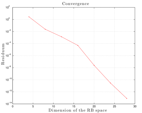
Figure 2: Convergence in function of the dimension of the reduced basis space for a parameter ${k}$ under ${{M}}=0.3$.

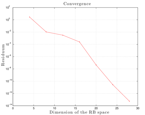
Figure 3: Convergence in function of the dimension of the reduced basis space for a parameter ${k}$ under ${{M}}=0.4$.

Table 1: Residuum, computational costs of the off-line stage and one Galerkin solution for ${{M}}=0.3$ and ${{M}}=0.4$ according to the dimension of the reduced basis space.

	${{M}}=0.3$			${{M}}=0.4$
Dimension	Residuum	${\mathcal{C}}_{\scriptsize\mbox{off}}$	${\mathcal{C}}_{\scriptsize\mbox{G}}$	Residuum	${\mathcal{C}}_{\scriptsize\mbox{off}}$	${\mathcal{C}}_{\scriptsize\mbox{G}}$
4	$2.7627$	789.4	6.37705	$2.8557$	793.9	6.42678
8	$2.3673\times 10^{-2}$	1581.1	6.36272	$1.0615\times 10^{-2}$	1590.0	6.41576
12	$1.3459\times 10^{-3}$	2370.7	6.37737	$3.1121\times 10^{-3}$	2384.2	6.37039
16	$4.9738\times 10^{-5}$	3163.7	6.37565	$2.4937\times 10^{-4}$	3181.8	6.38359
20	$2.4432\times 10^{-8}$	3958.1	6.38165	$4.4107\times 10^{-8}$	3979.2	6.42344
24	$2.9129\times 10^{-11}$	4750.5	6.38063	$2.6859\times 10^{-11}$	4778.2	6.43455
28	$8.0662\times 10^{-14}$	5542.6	6.37059	$5.4560\times 10^{-14}$	5575.4	6.44458

4.1.2 Two Parameters of Wave and Mach Numbers

Let $\mathcal{D}_{\scriptsize\mbox{train}}={\left\{{{k}_{i}}\right\}}_{i=1}^{N_{1}}\times{\left\{{{{M}}_{j}}\right\}}_{j=1}^{N_{2}}$ made of the product of an $N_{1}$ terms of an arithmetic progression sequence from ${k}_{\min}$ to ${k}_{\max}$, and an $N_{2}$ terms of an arithmetic progression sequence from ${{M}}_{\min}$ to ${{M}}_{\max}$. Here $N_{1}$, $N_{2}$, ${k}_{\min}$, ${k}_{\max}$, ${{M}}_{\min}$ and ${{M}}_{\max}$ are numbers of samples in wave number ${k}$ and Mach number $M$ in (5), lower bounds and upper bounds of them, respectively. We set $N_{1}=N_{2}=10$, ${k}_{\max}=12$, ${k}_{\min}=8$, ${{M}}_{\max}=0.4$ and ${{M}}_{\min}=0.2$ in the mesh of size $h=0.025$.

The computational costs at offline ${\mathcal{C}}_{\scriptsize\mbox{off}}$, online ${\mathcal{C}}_{\scriptsize\mbox{on}}$ and one full Galerkin method ${\mathcal{C}}_{\scriptsize\mbox{G}}$ are 23281, 0.1099 and 25.538, respectivley. We see that the computational benefit of the RBM occurs when the computations are more than or equal to the marginal number ${n^{*}}=916$. We also see that the computational cost at the on-line stage is $230$ times shorter than that of one computation by the Galerkin method, where the number of the speed up comes from the ratio of the Galerkin cost ${\mathcal{C}}_{\scriptsize\mbox{G}}$ to the on-line cost. This is very promising aspect of the RBM such that the speed up makes it possible to apply the RBM to the practical problems under many and fast computational loads.

Figure 4 shows the real part of the solution by the reduced basis of dimension $N=10$ and the absolute error between the RBM solution and the exact solution for fixed parameters ${{M}}=0.3$ and ${k}=10$. The errors between the RBM solution and the exact one are $0.0278$ in $L^{\infty}({\Omega})$, $0.0223$ in $L^{2}({\Omega})$, and $0.0320$ in $H^{1}({\Omega})$.

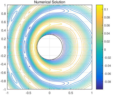
Figure 4: Real part of the numerical solution by the 10 dimensional RBM chosen from 100 samples among $[8,12]\times[0.2,0.4]$ when ${{M}}=0.3$ and ${k}=10$.

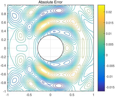
Figure 5: Absolute error of the numerical solution by the 10 dimensional RBM chosen from 100 samples among $[8,12]\times[0.2,0.4]$ when ${{M}}=0.3$ and ${k}=10$.

4.2 Unbounded Domain

The duct in Figure 6 has an elliptical hole whose major and minor axes are $a=0.3$ and $b=0.25$, and center is at the origin. We set $x_{-}=-1$, $x_{+}=1$, $L=1$ and $\sigma_{0}=15$ for the damping function ${\alpha}(x)$ in (9). We generate meshes for ${\tilde{\Omega}}$ of mesh size $h=0.0381$ by Gmsh, which has $16907$ nodes and $33262$ elements. We treat the wave and Mach numbers as parameters. We use 16 training samples among $[8,12]\times[0.2,0.4]$ and choose 10 basis from them. The computational costs at offline ${\mathcal{C}}_{\scriptsize\mbox{off}}$, online ${\mathcal{C}}_{\scriptsize\mbox{on}}$ and one full Galerkin method ${\mathcal{C}}_{\scriptsize\mbox{G}}$ are 4899, 0.15763 and 188.2764, respectivley. The marginal number is ${n^{*}}=27$ and the computational speed by the on-line stage is at least 1,100 faster than that by the usual Galerkin method.

Figure 6: Bounded domain ${{\Omega}_{b}}$ and PML domain ${\Omega}_{L}^{\scriptsize{\mbox{PML}}}\cup{\Omega}_{R}^{\scriptsize{\mbox{PML}}}$.

The errors between the 10 dimensional RBM solution and the exact one are $0.0682$ in $L^{\infty}({\Omega})$, $0.0248$ in $L^{2}({\Omega})$, and $0.4012$ in $H^{1}({\Omega})$. The $H^{1}({\Omega})$ error is higher than that for the bounded domain, which is caused by the small number of training samples.

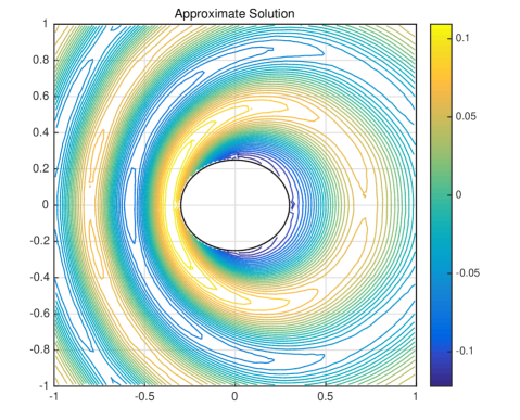
Figure 7: Real part of the numerical solution by the 10 dimensional RBM selected from 16 samples among $[8,12]\times[0.2,0.4]$ in ${\Omega}_{b}$ when ${{M}}=0.3$ and ${k}=10$.

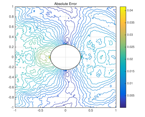
Figure 8: Absolute error of the numerical solution by the 10 dimensional RBM selected from 16 samples among $[8,12]\times[0.2,0.4]$ in ${\Omega}_{b}$ when ${{M}}=0.3$ and ${k}=10$.

5 Conclusion

We test the RBM for the convected Helmholtz equation. The physical parameters are expressed as coefficients of the equation. After these tests, we confirm that the RBM works well and gives us the benefit of fast computation at least 100 times than the usual computational method does. In the implementation, we use the error estimator based on the primal norm of the error.

References

- [1] M. Barrault, Y. Maday, N. C. Nguyen, and A. T. Patera, An ‘empirical interpolation’ method: application to efficient reduced-basis discretization of partial differential equations, C. R. Acad. Sci. Paris Ser. I 339(2004), no.9, 667–672.
- [2] E. Bécache, A.-S. Bonnet-Ben Dhia, and G. Legendre, Perfectly matched layers for the convected Helmholtz equation, SIAM J. Numer. Anal. 42(2004), no.1, 409–433.
- [3] P. Binev, A. Cohen, W. Dahmen, R. A. DeVore, G. Petrova, and Prz. Wojtaszczyk, Convergence rates for greedy algorithms in reduced basis methods, SIAM J. Math. Anal. 43(2011), no.3, 1457–1472.
- [4] S. Boyaval, C. Le Bris, T. Lelièvre, Y. Maday, N. C. Nguyen, and A. T. Patera, Reduced basis techniques for stochastic problems, Arch. Comput. Methods Eng. 17(2010), 435–454.
- [5] S. Boyaval, C. Le Bris, Y. Maday, N. C. Nguyen, and A. T. Patera,A reduced basis approach for variational problems with stochastic parameters: Application to heat conduction with variable Robin coefficient, Comput. Methods Appl. Mech. Engrg. 198(2009), 3187–3206.
- [6] A. Buffa, Y. Maday, A. T. Patera, Chr. Prud’Homme, and G. Turinici, A priori convergence of the greedy algorithm for the parametrized reduced basis method, ESAIM Math. Model. Numer. Anal. 46(2012), no.3, 595–603.
- [7] Y. Chen, J. S. Hesthaven, Y. Maday, and J. Rodríguez, Certified reduced basis methods and output bounds for the harmonic Maxwell’s equations, SIAM J. Sci. Comput. 32(2010), no.2, 970–996.
- [8] Y. Chen, J. S. Hesthaven, Y. Maday, J. Rodríguez, and X. Zhu, Certified reduced basis method for electromagnetic scattering and radar cross section estimation, Comput. Methods Appl. Mech. Engrg. 233-236(2012), 92–108, 2012.
- [9] M. Drohmann, B. Haasdonk, and M. Ohlberger, Reduced basis approximation for nonlinear parametrized evolution equations based on empirical operator interpolation, SIAM J. Sci. Comput. 34(2012), no.2, A973–A969.
- [10] C. Geuzaine and J. F. Remacle, Gmsh: a three-dimensional finite element mesh generator with built-in pre- and post-processing facilities, Int. J. Numer. Meth. Eng. 79(2009), no.11, 1309–1331.
- [11] B. Haasdonk, K. Urban, and B. Weiland, Reduced basis methods for parametrized partial differential with stochastic infulences using the Karhunen-Loève expansion, SIAM/ASA J. Uncertain. Quantif. 1(2013), 79–105.
- [12] F. Q. Hu, On absorbing boundary conditions for linearized Euler equations by a perfectly matched layer, J. Comput. Phys. 129(1996), 201–219.
- [13] Chr. Jäggli, L. Iapichino, and G. Rozza, An improvement on geometrical parameterizations by transfinite maps, C. R. Acad. Sci. Paris Ser. I, 352(2014), 263–268.
- [14] Y. Maday, A. T. Patera, and G. Turinici, A priori convergence theory for reduced-basis approximations of single-parametric elliptic partial differential equations, J. Sci. Comput. 17(2002), 437–446.
- [15] A. Manzoni, A. Cohen, and G. Rozza, Shape optimization for viscous flows by reduced basis methods and free-form deformation, Int. J. Numer. Meth. Fluids, 70(2012), 646–670.
- [16] F. Negri, A. Manzoni, and G. Rozza, Reduced basis approximation of parametrized optimal flow control problems for the stokes equations, Comput. Math. Appl. 69(2015), 319–336.
- [17] F. Negri, G. Rozza, A. Manzoni, and A. Quarteroni, Reduced basis method for parametrized elliptic optimal control problems, SIAM J. Sci. Comput. 35(2013), no.5, A2316–A2340.
- [18] P. Pacciarini and G. Rozza, Stabilized reduced basis method for parametrized advection-diffusion PDEs, Comput. Methods Appl. Mech. Engrg. 274(2014), 1–18, 2014.
- [19] S. Park and I. Sim, Analysis of PML method for stochastic convected Helmholtz equation, submitted.
- [20] A. T. Patera and G. Rozza, Reduced basis approximation and a posteriori error estimation for parametrized partial differential equations, Version 1.0, MIT Pappalardo Graduate Monographs in Mechanical Engineering, 2007.
- [21] J. Pomplun and F. Schmidt,Accelerated a posteriori error estimation for the reduced basis method with application to 3D electromagnetic scattering problems, SIAM J. Sci. Comput. 32(2010), no.2, 498–520.
- [22] A. Quarteroni, G. Rozza, and A. Manzoni. Certified reduced basis approximation for parametrized partial differential equations and applications, J. Math. Ind. 1(2011), Art. 3.
- [23] G. Rozza, D. B. P. Huynh, and A. T. Patera, Reduced basis approximation and a posteriori error estimation for affinely parametrized elliptic coercive partial differential equations, Arch. Comput. Methods Eng. 15(2008), no.3, 229–275.
- [24] D. Wirtz, D. C. Sorensen, and B. Haasdonk, A posteriori error estimation for DEIM reduced nonlinear dynamical systems, SIAM J. Sci. Comput. 36(2014), no.2, A311–A338.