Tree-Cut for Probabilistic Image Segmentation

Abstract

This paper presents a new probabilistic generative model for image segmentation, i.e. the task of partitioning an image into homogeneous regions. Our model is grounded on a mid-level image representation, called a region tree, in which regions are recursively split into subregions until superpixels are reached. Given the region tree, image segmentation is formalized as sampling cuts in the tree from the model. Inference for the cuts is exact, and formulated using dynamic programming. Our tree-cut model can be tuned to sample segmentations at a particular scale of interest out of many possible multiscale image segmentations. This generalizes the common notion that there should be only one correct segmentation per image. Also, it allows moving beyond the standard single-scale evaluation, where the segmentation result for an image is averaged against the corresponding set of coarse and fine human annotations, to conduct a scale-specific evaluation. Our quantitative results are comparable to those of the leading gPb-owt-ucm method, with the notable advantage that we additionally produce a distribution over all possible tree-consistent segmentations of the image.

The image segmentation problem can be formalized as partitioning an image into a set of non-overlapping regions so that each region is (in some sense) homogeneous. Mathematically, this can be expressed in terms of an objective function

$$J(R)=\sum_{i\in R}\ell(Y_{i})-c(R),$$ (1)

where $R$ denotes the set of regions, $\ell(Y_{i})$ is the log likelihood of the image data $Y_{i}$ that belongs to region $i$, and $c(R)$ is a penalty term that e.g. penalizes the number of regions used.

For input data with a one-dimensional ordering (e.g. a time series), this problem is referred to as a changepoint problem, and dynamic programming can be used to find the optimal segmentation, see e.g. [1]. However, such an approach is not tractable in 2-d for image regions of arbitrary shape. Instead, given a set of superpixels (i.e. an oversegmentation) of the image, we make use of a region tree with superpixels as leaves, and with regions being obtained as cuts in the tree. Given the region tree, we formalize image segmentation as sampling from the posterior over cuts in the tree from a generative model. In this way, our image segmentation amounts to selecting a segmentation from many possible multiscale segmentations encoded by the region tree. Due to the tree structure, MAP inference and sampling for the cuts is exact, and formulated using dynamic programming. An example of tree-cut in operation is shown in Figure 1, with tuning for coarse and fine segmentations. Some posterior samples are shown in Figure 2.

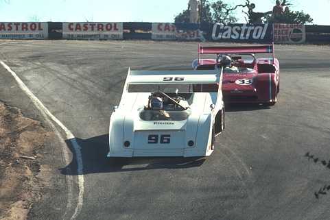
(a)

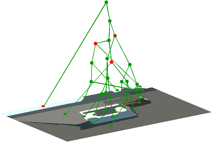
(c)

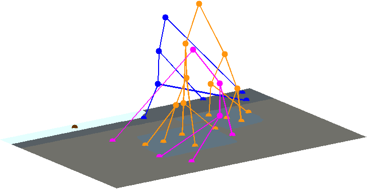
(e)

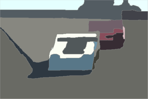
(b)

(d)

(f)

Figure 1: Illustration of tree-cut (best viewed in color). (a) The original image. (b) There are 18 superpixels corresponding to the leaves of the region tree. (c)-(d) The region trees showing the active nodes (highlighted as red) after tree-cutting with different parameters. (e)-(f) The resulting forests and segmentations. The nodes on the same subtree are rendered with the same color. The coarse segmentation (e) has 4 regions, and the fine segmentation (f) has 7 regions. These were obtained with $p=0.99$ and $p=0.90$ respectively, and $\lambda=2\times 10^{-4}$; the meaning of these parameters is explained in section 1.

The primary contribution of this paper is the formulation of a principled and efficient probabilistic hierarchical model for image segmentation. Our model is generative, and thus allows for probabilistic sampling of image segmentations at a particular scale of interest, where the scale (e.g., coarse or fine) can be defined in terms of a number of regions in the resulting segmentation. This can be efficiently done by training only one parameter of our model on ground-truth segmentations of a desired scale. Our second contribution is that we generalize the common notion that there should be only one correct segmentation result per image. This allows us to move beyond the evaluation methods of [3] which average their result over the set of human annotations for a given image. In contrast, we provide a more fine-grained evaluation, e.g. by tuning our model to provide coarser or finer segmentations as per user specifications during training.

The remainder of the paper is organized as follows: In section 1 we describe the model over tree-cuts, the likelihood for regions, and efficient computations for MAP inference and sampling from the posterior over segmentations. We also include a discussion of related work. In section 2 we describe experiments on the BSDS datasets, including an evaluation of tuning our method to provide coarser or finer segmentations. We conclude with a discussion and directions for future work.

1 The Model

We first describe the model over tree-cuts, and algorithms for MAP and sampling inference on the tree. We then discuss the model used for the likelihood of image regions, how parameters in the model can be set, and related work.

1.1 Probabilities over tree cuts

We start with a region tree $T$ whose leaves correspond to a superpixel decomposition of the image. A region is defined by activating a node in the tree—this means that all of the superpixels governed by that node are considered to form one region. An active node corresponds to a cut in the tree, in that it disconnects its subtree from the remainder of the tree. A valid segmentation is obtained by activating a set of nodes so that there is only one node active per path from leaf to root (see e.g. [4, sec 4.1]), which we refer to as the OONAPP constraint.

A convenient way of generating segmentations obeying the OONAPP constraint is in a top-down fashion. Starting at the root, we can either activate that node (making the whole image one region), or leave the root inactive and move down to consider its children, by removing the edges between them and the root. At each child we face the same question of whether to activate or not. If this process continues down and we reach a leaf node then it must be activated, otherwise that superpixel would not be accounted for in the image.

We can ascribe probabilities to each configuration in the following manner. Let each node $i$ have an activation probability $p_{i}$ and an associated binary variable $z_{i}$, with prior probability $p(z_{i}=1)=p_{i}$. The $z$ variables are collected into a vector $\mathbf{z}$. Let the set of active nodes in $T$ be denoted as $A_{T}$, the nodes lying above the active nodes as $A^{-}_{T}$, and those below $A_{T}$ as $A^{+}_{T}$. The $z$ variables are set to 1 for active nodes and those in $A^{+}_{T}$, and to 0 for nodes in $A^{-}_{T}$. Then we have that

$$p(\mathbf{z})=\prod_{i\in A^{-}_{T}}p(z_{i}=0)\prod_{j\in A_{T}}p(z_{j}=1)\prod_{k\in A^{+}_{T}}\delta(z_{k}=1).$$ (2)

Note that the nodes in $A^{+}_{T}$ are turned on with probability 1 given $A_{T}$. In relation to eq. (1), the penalty term $c(R)$ would be identified as $-\log p(\mathbf{z}|A_{T})$.

It is easy to show that this construction defines a valid probability distribution over tree-cuts. Consider the subtree rooted at node $i$, and assume that the distribution over configurations for the subtrees are valid probability distributions. With probability $p_{i}$ we have $z_{i}=1$ (and all of the $z$ variables below it are also turned on, as per eq. (2)). With probability $1-p_{i}$ we have $z_{i}=0$ and the probability is evaluated as the product over the configurations of the children. Let $\mathbf{z}^{i}$ denote $z_{i}$ and all of the $z$ variables below it in the tree. To check that $\sum_{\mathbf{z}^{i}}p(\mathbf{z}^{i})=1$, break this sum up into sums over $z_{i}$ and over the variables in each subtree. By summing over $z_{i}$ and letting $\mathbf{z}^{j}$ denote the $z$ variables in the subtree rooted at node $j$ (a child of node $i$), we obtain

$$\sum_{\mathbf{z}^{i}}p(\mathbf{z}^{i})=p_{i}+(1-p_{i})\prod_{j\in\mathrm{ch}(i)}\left(\sum_{\mathbf{z}^{j}}p(\mathbf{z}^{j})\right)=1$$ (3)

based on the induction hypothesis that the subtrees are valid probability distributions. The proposition in eq. (3) holds by the base case, i.e. that the leaf nodes have their $p$ variables set to 1.

1.2 Computing the total probability of the data summing over all configurations

Let the likelihood of a region $i$ with node $i$ being active be denoted as $p(Y_{\Delta i})$. At any non-leaf node we can explain the data governed by it either by making it the active node, or by passing the responsibility to its children. Thus the total probability $p(Y_{i})$ of explaining the data governed by node $i$ is given by the recursive formula

$$p(Y_{i})=\sum_{\mathbf{z}^{i}}p(\mathbf{z}^{i})p(Y_{i}|\mathbf{z}^{i})=p_{i}p(Y_{\Delta i})+(1-p_{i})\prod_{j\in\mathrm{ch}(i)}p(Y_{j}),$$ (4)

where as above we have decomposed the sum into terms over $z_{i}$ and the remaining $z$ variables. This recurison “bottoms out” for a leaf node $k$ with $p(Y_{k})=p(Y_{\Delta k})$, because $p_{k}=1$ for leaf nodes. Thus if $Y$ denotes all of the image data, we can compute $p(Y)$ at the root node by a bottom up pass through the tree.

1.3 Computing the MAP configuration, and sampling from $p(\mathbf{z}|Y)$

We now wish to find a valid OONAPP configuration $\mathbf{z}^{*}$ that maximizes $p(\mathbf{z}^{*}|Y)$. Note that

$$p(\mathbf{z}|Y)=\frac{1}{p(Y)}\;p(\mathbf{z})\prod_{j\in A_{T}(\mathbf{z})}p(Y_{\Delta_{j}}),$$ (5)

where $p(\mathbf{z})$ is defined as per eq. (2).

Let $p^{*}(Y_{i})$ denote the likelihood of the data governed by node $i$ under the optimal choice of $z$ variables at and below node $i$. At node $i$ we can either explain all of the data in the subtree with probability $p_{i}p(Y_{\Delta i})$ (the “direct” contribution), or make use of the children (the “indirect” contribution). Thus

$$p^{*}(Y_{i})=\max[p_{i}p(Y_{\Delta i}),\;(1-p_{i})\prod_{j\in\mathrm{ch}(i)}p^{*}(Y_{j})].$$ (6)

For leaf nodes $p^{*}(Y_{k})=p(Y_{\Delta k})$. Again we can compute $p^{*}(Y)$ by a bottom-up pass through the tree, and obtain the optimal MAP configuration by a top-down backtracking pass having stored the argmax decisions made at each node in the tree.

(a)

(b)

(c)

(d)

Figure 2: Sampling from $p(\mathbf{z}|Y)$. (a) The original images which have 548 and 1263 superpixels respectively. (b)-(d) Samples with 39, 32 and 44 cuts for the first image and with 64, 64 and 69 cuts for the second image. The colors are selected as the median colors of the regions.

Sampling from $p(\mathbf{z}|Y)$. At the root we have computed the direct contribution $p_{D}(Y_{r})=p_{r}p(Y_{\Delta r})$ and the indirect contribution $p_{I}(Y_{r})=(1-p_{r})\prod_{j\in\mathrm{ch}(r)}p(Y_{j})$. To sample over tree configurations we first sample the root with $p(z_{r}=1|Y_{r})=p_{D}(Y_{r})/[p_{D}(Y_{r})+p_{I}(Y_{r})]$. If $z_{r}$ is active we stop, alternatively we recurse into the subtrees, and sample there on the same basis. The variety of segmentations that can be obtained by sampling is illustrated in Figure 2.

It is also possible to compute other quantities via message passing on the tree, such as the marginals $p(z_{i}|Y)$.

1.4 Likelihoods

We need to define a likelihood model for data under a given node. The simplest assumption is to assume that all pixels in the region are drawn from a Gaussian distribution. Let there be pixels $\mathbf{y}^{1},\ldots,\mathbf{y}^{N}$. These are $D=3$ dimensional vectors as they are RGB values (other colour spaces are possible). The maximum likelihood solutions for the mean and covariance matrix of this data are the empirical mean $\hat{\boldsymbol{\mu}}=\frac{1}{N}\sum_{n=1}^{N}\mathbf{y}^{n}$ and $\hat{\Sigma}=\frac{1}{N}\sum_{n=1}^{N}(\mathbf{y}^{n}-\hat{\boldsymbol{\mu}})(\mathbf{y}^{n}-\hat{\boldsymbol{\mu}})^{T}$. The log likelihood of the data under this model is

$$L =-\frac{1}{2}\sum_{n=1}^{N}[D\log(2\pi)+\log|\hat{\Sigma}|+(\mathbf{y}^{n}-\hat{\boldsymbol{\mu}})^{T}\hat{\Sigma}^{-1}(\mathbf{y}^{n}-\hat{\boldsymbol{\mu}})]$$

$$=-\frac{N}{2}[D\log(2\pi)+\log|\hat{\Sigma}|]-\frac{1}{2}\mathrm{tr}[\hat{\Sigma}^{-1}\sum_{n}(\mathbf{y}^{n}-\hat{\boldsymbol{\mu}})(\mathbf{y}^{n}-\hat{\boldsymbol{\mu}})^{T}]$$

$$=-\frac{N}{2}[D\log(2\pi)+\log|\hat{\Sigma}|]-\frac{N}{2}\mathrm{tr}(I_{D})=-\frac{N}{2}[D\log(2\pi)+\log|\hat{\Sigma}|+D].$$

Instead of maximizing over $\boldsymbol{\mu}$ and $\Sigma$, it would be possible to integrate them out via a Bayesian analysis; a Normal-Wishart prior would be conjugate to the likelihood. More complex likelihoods involving spatial correlations between pixels are discussed in sec. 3.

In HMMs for speech recognition it is well-known [5] that it can be useful to adjust the relative scaling of the likelihood and structural terms, as the likelihood term arises from continuous observations, while the structural terms arise from discrete transition probabilities. In the recursive equations this is easily handled by simply multiplying the log likelihood by a factor $\lambda>0$.

In order to assess the effect of various likelihoods, we also devised a “ground-truth” (GT) likelihood term, taking account of the segment labels in the annotations. Let $n_{ij}$ denote the number of labels of type $j$ in region $i$, and let there be $m$ different labels. We can ascribe a probability $\pi_{ij}$ for label $j$ in region $i$, and the log-likelihood under this model is maximized by setting $\hat{\pi}_{ij}=n_{ij}/n_{i.}$ with $n_{i.}=\sum_{k}n_{ik}$. Thus we obtain a GT-likelihood of

$$L^{GT}_{i}=n_{i.}\sum_{j=1}^{m}\hat{\pi}_{ij}\log\hat{\pi}_{ij}.$$ (7)

Note that this “ground truth” likelihood still omits spatial correlations, so although it is very likely to be optimistic relative to the independent Gaussian model, it may not be an upper bound what can be achieved.

1.5 Setting the $p$ parameters

In the above formulation each internal node $i$ has an associated parameter $p_{i}$; the corresponding $p$ for the leaves must be set to 1. Note also that the region tree is different for each input image. Thus it is not possible to learn the $p_{i}$ parameters directly by accumulating information over images.

One simple approach is to set a unique $p$ globally for a set of images and segmentations, so as to optimize some measure of performance, such as the covering score (see eq. (8)). Note that maximization of the log likelihood $\log p(Y)$ wrt $p$ would lead to setting $p=0$, as one can always obtain a higher likelihood by having a specific model for each superpixel rather than merging them.

An interesting alternative would be to predict $p_{i}$ based on information in the tree, such as the UCM scores (explained in sec. 1.6 below) of a node, its children and its parent, and the fraction of nodes in the tree that are governed by it. A suitable predictor would be e.g. logistic regression. In this case the model would be a hierarchical conditional random field (CRF), as the $p$ parameters would be set on the basis of the image data. We leave this direction for future work.

1.6 Related Work

There are a vast number of papers on the topic of image segmentation, going back decades. For a summary see e.g. [6, ch. 5] and [7, ch. 14]. Generally these are based on: (a) Clustering of color and texture features with mixture models, (b) Distribution-mode finding, (c) Graph partitioning, or (d) Boundary detection and closing the boundaries.

The work by Arbelaez et al. [3] is a notable example of boundary-detection based methods. They first run the gPb boundary detector to produce a boundary response map. The detected boundaries are then closed using Oriented Watershed Transform (OWT), resulting in regions organized in an Ultrametric Contour Map (UCM). In the UCM each region is labelled with a weight value. By thresholding the UCM at a particular weight, usually denoted by $k$, one obtains a segmentation at scale $k$. Varying $k$ produces a strict hierarchy of regions, which can be organized in a region tree by their nesting properties. We refer to this work as the gPb-owt-ucm method.

It is worth noting that gPb-owt-ucm does not define a distribution over segmentations, unlike our model. A particular value of $k$ (as obtained e.g. from a training set) selects one segmentation in the tree. Other multiscale-segmentation approaches also use a single threshold to identify the “right” scale of segmentation (e.g. [8, 9, 10]).

In general, one should make a distinction between image segmentation, which is an unsupervised procedure, and semantic scene segmentation, where the aim is to label each (super)pixel with one of a discrete set of object class labels, e.g. sky, vegetation, vehicle etc. The “Pylon model” of [11] uses a notion of cuts in a region tree to define possible segment labellings, and then carries out inference in the tree to find the optimal cuts. Our cuts and the OONAPP constraint are similar to their work, but our task – image segmentation as opposed to semantic segmentation – is entirely different.

There has also been much prior work on using tree-structured models for tasks other than image segmentation. For example [12] used a quad-tree structured belief network to carry out a semantic segmentation task; a disadvantage of their approach is that the quad-tree structure does not depend on the input image structure, and so can lead to “blocky” artifacts. The Dynamic Trees work of [13] aimed to address this problem by using a prior distribution over many candidate trees. However, this meant that approximate variational inference had to be used; in contrast we can use exact inference in one data-driven tree. The Recursive Neural Network of [14] learns to merge agglomeratively a set of superpixels to produce a tree structure. However, note that the final segmentation depends only on the learned features applied on a superpixel-by-superpixel basis.

2 Experiments

Our experiments are carried out on the widely-used Berkeley Segmentation Dataset (BSDS) [3]. There are two versions, the BSDS300 dataset (which consists of 200 training and 100 test images), and the BSDS500, which has an additional 200 test images, with the BSDS300 being used as training/validation data. Each of the images was segmented by several human annotators.

To produce one segmentation for each image we carry out MAP inference, as described in sec. 1.3.

Evaluation metrics: There are a number of ways to evaluate the agreement between the output of a segmentation algorithm and the human annotations. Following [3] we consider the segmentation covering score (COV), the variation of information (VI) [15], and the Probabilistic Rand Index (PRI) [16]. Notice that VI and the Rand index were introduced for the evaluation of clusterings, i.e. they are not specialized to image segmentation (with its spatial aspects).

The intersection-over-union (IoU) score between two regions $R$ and $R^{\prime}$ is defined as $\mathrm{IoU}(R,R^{\prime})=|R\cap R^{\prime}|/|R\cup R^{\prime}|$. The covering score of a segmentation $S$ by a segmentation $S^{\prime}$ is then given by

$$COV(S\rightarrow S^{\prime})=\frac{1}{N}\sum_{R\in S}|R|\max_{R^{\prime}\in S^{\prime}}\mathrm{IoU}(R,R^{\prime}).$$ (8)

When evaluating segmentations, Arbelaez et al. [3] consider two situations, which they term optimal dataset scale (ODS) and optimal image scale (OIS). The difference is that their UCM scale parameter $k$ is set for the whole dataset in ODS, while it is optimized on a per image basis (while averaging over the different segmentations) for OIS.

We consider two experiments. In the first (sec. 2.1) we use the same evaluation criteria as in [3]. Secondly, in sec. 2.2 we show how the methods can be tuned on specific sets of segmentations so as to produce methods that can e.g. provide coarser or finer segmentations.

BSDS300     Covering PRI VI ODS OIS ODS OIS ODS OIS Human 0.73 0.73 0.87 0.87 1.16 1.16 gPb-owt-ucm 0.587 0.646 0.808 0.852 1.650 1.461 Tree-cut 0.583 0.651 0.793 0.853 1.646 1.437 Tree-cut (GT) 0.692 0.715 0.877 0.894 1.364 1.165

BSDS500     Covering PRI VI ODS OIS ODS OIS ODS OIS Human 0.72 0.72 0.88 0.88 1.17 1.17 gPb-owt-ucm 0.587 0.647 0.826 0.856 1.687 1.469 Tree-cut 0.592 0.650 0.810 0.857 1.633 1.448 Tree-cut (GT) 0.688 0.707 0.881 0.890 1.391 1.280

Table 1: Results for the BSDS300 and BSDS500 datasets. The Human and gPb-owt-ucm results are as in [3], except that for gPb-owt-ucm we have re-calculated them to 3 dec pl. Between gPb-owt-ucm and TC the best performing method is shown in bold; for covering and PRI higher numbers are better, while for VI lower is better. The tree-cut (GT) results use the ground-truth likelihood as described in sec. 1.4.

2.1 BSDS-style evaluation

The MAP results for the BSDS-style data evaluation are shown in Table 1, for both the BSDS300 and BSDS500 datasets. These are results on the respective test sets, for ODS cases the parameters were optimized on the training set. The results on covering, PRI and VI for gPb-owt-ucm and tree-cut (TC) are basically very similar, with the numbers lying within about 1% of each other. We also conducted experiments sampling 500 segmentations for a given image rather than computing the MAP; the mean scores for here were very similar to the MAP result. To give some idea of the variability, for the covering score the average standard deviation (wrt the 500 samples) was around 0.01.

As would be expected, using the “ground-truth” likelihood (as explained in sec. 1.4) does improve the performance of tree-cut markedly, which suggests that it could be beneficial to look for better likelihood models (see also the discussion in sec. 3). We observe that the OIS measures for tree-cut GT are very close to human performance, which makes sense given that it is making use of the information in the human-provided segmentations.

For interest we report the parameters for the gPb-owt-ucm and TC models that maximize the ODS covering score. For gPb-owt-ucm we searched over a grid of 100 equally-spaced $k$ values from $0.01$ to $1.00$. For our tree-cut method we considered scaling factors $\lambda$ for the likelihood (see sec. 1.4) from $10^{-4}$ to $10^{-3}$ in steps of $10^{-4}$. For $p$ we considered 100 values between 0.0001 and 0.9999, with denser gridpoints towards the higher values (nearer to 1). The optimal values for BSDS300 were $k=0.170$, $p=0.968$, $\lambda=0.0004$. For BSDS500 the optimal values were $k=0.170$, $p=0.971$, $\lambda=0.0005$.

gPb-owt-ucm

Model	Data source
trained on	Coarse	Medium	Fine
Coarse	0.620	0.562	0.539
Medium	0.589	0.572	0.564
Fine	0.559	0.568	0.569
All	0.589	0.572	0.564

Tree-cut

Model	Data source
trained on	Coarse	Medium	Fine
Coarse	0.645	0.574	0.512
Medium	0.606	0.585	0.551
Fine	0.540	0.561	0.561
All	0.617	0.583	0.545

Table 2: Covering scores for the coarse/medium/fine experiments.

2.2 Coarser and finer segmentations

The scores in section 2.1 are obtained by averaging over the set of segmentations available for a given image. However, it is natural to want to be able to control the level of detail obtained, and this can be done in our method by varying the $p$ parameter, and for gPb-owt-ucm by varying $k$.

To explore this aspect, we divided the BSDS500 images into three groups, which we refer to as coarse, medium and fine segmentations. Coarse images contain 1-8 segments, medium have 9-31, and fine images contain 32 or more segments. There are 168, 284 and 144 images in these classes respectively in the trainval set, and 99, 183 and 109 on the test set.

Models were trained (by grid search over the parameters as described above) to optimize the covering score on one of the groups of training data. The test-set covering scores reported in in Table 2 were evaluated on the 200 BSDS500 test images. For both the TC and gPb-owt-ucm models it is notable that the performance is better when training has taken place on the same type of data as is used for testing (as seen by the diagonal elements in the tables being higher than other ones in the same column). The performance differences inside the columns are generally larger for the TC method than for gPb-owt-ucm; for example for testing on coarse data, the TC difference is 0.105, while the gPb-owt-ucm difference is 0.061. This implies that the effect of tuning is stronger for TC than gPb-owt-ucm. Comparing with the last line in the tables where either method was trained on all of the data (as in sec. 2.1), we see that it never hurts performance to train on a specific subset of data (coarse/medium/fine) when testing on the same division.

For gPb-owt-ucm, the optimal $k$ values obtained were 0.25, 0.17 and 0.13 for coarse, medium and fine training respectively. These make sense in that coarser segmentations correspond to higher UCM values. For tree-cut for greater interpretability we have chosen to fix $\lambda=0.0009$; the corresponding values of $p$ are $0.9999$, $0.9963$ and $0.968$ resp. As would be expected coarser segmentations lead to $p$ values nearer to 1 (as this gives a higher probability of stopping at higher levels in the tree, see sec. 1.1)

3 Discussion

Our main contribution has been to introduce a principled and efficient hierarchical model for image segmentation, extending the ideas from 1-d changepoint analysis to images. The results in sec. 2.1 show that this produces very similar results to the gPb-owt-ucm method in terms of the standard BSDS evaluation scores using the MAP segmentation. A great advantage is that our method does not produce just one segmentation, but can sample over segmentations in order to reflect different possible interpretations.

Our second contribution is to delve deeper into the image segmentation task, addressing the fact the BSDS data contains multiple segmentations of a given image. We have shown in sec. 2.2 how the tree-cut and gPb-owt-ucm methods can be tuned to produce coarser or finer segmentations, and have evaluated how this affects the segmentation covering scores.

There are a number of directions in which this work can be extended. Firstly, our model is generative, defining a distribution $p(Y,\mathbf{z})$ given a tree. It would be possible to create a discriminative version that aims to optimize $p(\mathbf{z}|Y)$ based on training set segmentations, in the spirit of [4] (but note that their work primarily addresses the semantic segmentation problem, not image segmentation).

Secondly, the independent-pixel Gaussian likelihood used in sec. 1.4 is very simple, and richer models that take spatial correlations into account could be used. For example one could use a Gaussian Field of Experts model [17], a Gaussian process model with special features for modelling image textures [18], or a conditional autoregressive (CAR) model, where each pixel is predicted on the basis of some context (usually taken to be above and to the left). However, using such models would greatly increase the computational cost of model fitting.

Thirdly, setting $p$ values globally in the tree is very simple, and it would be very interesting to predict these values from information available in the tree, as discussed in sec. 1.5. This could also mean selecting different values of in different parts of the image, which would be useful for complex scenes with large variations in object sizes (e.g., due to large differences in their distances from the camera). Finally, our method and gPb-owt-ucm both use a single, data-driven tree. However, it is natural to consider a distribution over possible trees, see e.g. the work on Dynamic Trees in [13]. One way to incorporate this idea in the tree-cut model is to use a number of different trees $T_{1},\ldots,T_{m}$, and sample segmentations from each of them. Their relative weights could be obtained via the likelihood $p(Y|T_{i})$ as computed in sec. 1.2.

Acknowledgments

We thank Glencora Borradaile for helpful discussions. CW thanks Rich Zemel for a conversation about the importance of producing multiple image segmentations. CW is an Associate Fellow of the Neural Computation and Adaptive Perception program of the Canadian Institite for Advanced Research (CIFAR). This work was supported in part by grants NSF IIS 1302700 and NSF DEB 1208272.

References

- [1] R. Killick, P. Fearnhead, and I. A. Eckley. Optimal Detection of Changepoints With a Linear Computational Cost. J. Amercian Stat. Soc., 107(500):1590–1598, 2012.
- [2] W. Wang, I. Pollak, T.-S. Wong, C.A. Bouman, M.P. Harper, and J. M. Siskind. Hierarchical Stochastic Image Grammars for Classification and Segmentation. IEEE Transactions on Image Processing, 15(10):3033–52, 2006.
- [3] P. Arbelaez, M. Maire, C. Fowlkes, and J. Malik. Contour detection and hierarchical image segmentation. IEEE Trans. Pattern Anal. Mach. Intell., 33(5):898–916, 2011.
- [4] N. Silberman, D. Sontag, and R. Fergus. Instance Segmentation of Indoor Scenes using a Coverage Loss. In ECCV, 2014.
- [5] L. R. Bahl, R. Bakis, F. Jelinek, and R. L. Mercer. Language-Model/Acoustic-Channel-Model Balance Mechanism. IBM Technical Disclosure Bulletin, 23(7B):3464–3465, 1980.
- [6] R. Szeliski. Computer Vision: Algorithms and Applications. Springer, 2010.
- [7] D. A. Forsyth and J. Ponce. Computer Vision: A Modern Approach. Prentice Hall, Upper Saddle River, New Jersey, 2003.
- [8] Hossein Mobahi, Shankar R. Rao, Allen Y. Yang, Shankar S. Sastry, and Yi Ma. Segmentation of Natural Images by Texture and Boundary Compression. International Journal of Computer Vision, 95(1):86–98, 2011.
- [9] Jingdong Wang, Yangqing Jia, Xian-Sheng Hua, Changshui Zhang, and Long Quan. Normalized tree partitioning for image segmentation. In CVPR, 2008.
- [10] S.X. Yu. Segmentation induced by scale invariance. In CVPR, 2005.
- [11] V. Lempitsky, A. Vedaldi, and A. Zisserman. Pylon model for semantic segmentation. In J. Shawe-Taylor, R.S. Zemel, P. Bartlett, F.C.N. Pereira, and K.Q. Weinberger, editors, Advances in Neural Information Processing Systems 24, pages 1485–1493. 2011.
- [12] C. A. Bouman and M. Shapiro. A Multiscale Random Field Model for Bayesian Image Segmentation. IEEE Transactions on Image Processing, 3(2):162–177, 1994.
- [13] A. J. Storkey and C. K. I. Williams. Image Modelling with Position-Encoding Dynamic Trees. IEEE Trans Pattern Analysis and Machine Intelligence, 25(7):859–871, 2003.
- [14] R. Socher, C. C. Lin, A. Y. Ng, and C. D. Manning. Parsing Natural Scenes and Natural Language with Recursive Neural Netw orks. In Proceedings of the 26th International Conference on Machine Learning (ICML), 2011.
- [15] M. Meila. Comparing Clusterings: An Axiomatic View. In Proceedings of the 22nd International Conference on Machine Learning, 2005.
- [16] R. Unnikrishnan, C. Pantofaru, and M. Hebert. Toward Objective Evaluation of Image Segmentation Algorithms. IEEE Trans Pattern Analysis and Machine Intelligence, 29(6):929–944, 2007.
- [17] Y. Weiss and W. T. Freeman. What makes a good model of natural images ? In CVPR 2007, 2007.
- [18] A. G. Wilson, E. Gilboa, A. Nehorai, and J. P. Cunningham. Fast Kernel Learning for Multidimensional Pattern Extrapolation. In Advances in Neural Information Processing Systems. MIT Press, 2014.