Single bunch transverse instability in a circular accelerator
with chromaticity and space charge

Abstract

The transverse instability of a bunch in a circular accelerator is elaborated in this paper. A new tree-modes model is proposed and developed to describe the most unstable modes of the bunch. This simple and flexible model includes chromaticity and space charge, and can be used with any bunch and wake forms. The dispersion equation for the bunch eigentunes is obtained in form of a third-order algebraic equation. The known head-tail and TMCI modes appear as the limiting cases which are distinctly bounded at zero chromaticity only. It is shown that the instability parameters depend only slightly on the bunch model but they are rather sensitive to the wake shape. In particular, space charge effects are investigated in the paper and it is shown that their influence depends on sign of wake field enhancing the bunch stability if the wake is negative. The resistive wall wake is considered in detail including a comparison of single and collective effects. A comparison of the results with earlier publications is carried out.

—————————————————————– ————-

CONTENTS

I.     Introduction
II.    Basic equations and definitions
III.   Exact solution for hollow bunch
IV.   Integral equations for multipoles
V.    Tree-modes model with chromaticity
VI.   Realistic bunch with arbitrary wake
VIA. Short rectangular wake
VIB. Resistive wake
VII.  Space charge effects
VIIA. Discussion
VIII. Conclusion
References
Appendix
——————————————————————————

I Introduction

Two kinds of single bunch transverse instability in circular accelerators are distinguished at present: the head-tail one and the transverse mode coupling instability (TMCI). First of them has been studied first by Pellegrini PEL and Sands SAND who were treating the transverse bunch oscillations as a combination of uncoupled multipoles $\,\propto\exp(im\phi)\,$ with $\,\phi\,$ as synchrotron phase. Role of synchrotron amplitude has been investigated later by Sacherer who was introducing the conception of radial modes SAH . A lot of papers dealing with this were published later, including reviews and books (see e.g. CHAO ; NG ). The most important conclusion is that the head-tail instability is possible at non-zero chromaticity only and depends on its sign.

Other type of instability was observed in many electron machines regardless of chromaticity and being primary referred as “transverse turbulence”. Its first explanation has been proposed by Kohaupt who used a simple model of two particles propelling each other through the mediation of constant wake fields KOH . Later the theory has been evolved on the base of Vlasov equation treating the instability as a result of reciprocal influence of neighboring pairs of the head-tail modes which frequencies approach each other due to a wake field, whence the term TMCI appears ZOT ; CHIN ; CHAO ; NG . Chromaticity has been ignored in these investigations as a factor of secondary importance. Some space charge effects has been considered later for both head-tail and TMCI instabilities BL ; BU ; B1 . However, specific models like the hollow bunch in the square potential well have been used in BL , and only high space charge limit was investigated in Ref. BL ; BU ; B1 .

An important observation is that, in all considered cases, the lowest multipoles $m=0,\,\pm 1$ or their combinations are the most prone to instability and pose a major threat to the accelerator operation. It is shown in this paper that the general theory can be essentially simplified and unified being restricted by these cases.

General 3-modes model is developed for this, providing simple analytical formulae for all types of single bunch instability. The model is built on the base of exact solutions for hollow bunch which are obtained in the paper without any additional assumptions like truncated multipole expansion. The dangerous modes are separated and extended to realistic distributions with arbitrary wake, chromaticity and space charge included.

It is shown that the instability parameters depend only slightly on the bunch shape being rather sensitive to the wake function form. Resistive wall wake is investigated especially to assign which effect is more dangerous in specific cases: either TMCI or collective mode instability. Chromaticity is taken into account in all the cases demonstrating an absence of clearly defined boundary between the head-tail instability (separated multipoles) and TMCI (coalesced multipoles). Space charge effects are studied with arbitrary ratio of betatron tune shift to synchrotron tune. In contrast with earlier papers BL ; BU ; B1 , the investigation is not restricted by simplified bunch models or by limiting cases only. It is shown that the space charge effect can be either advantageous or not for the bunch stability, dependent on the wake sign.

II Basic equations and definitions B1

Linear synchrotron oscillations are considered in this paper being characterized by amplitude $\,A\,$ and phase $\,\phi$, or by corresponding Cartesian coordinates:

$$\theta=A\cos\phi,\qquad u=A\sin\phi.$$ (1)

Thus $\,\theta\,$ is azimuthal deviation of the particle from the bunch center in the rest frame whereas the variable $u$ is proportional to the momentum deviation with respect to the central bunch momentum (proportionality coefficient is not a factor in this paper). Steady state of a bunch will be described by the distribution function $\,F(A)\,$ and by corresponding linear density

$$\rho(\theta)=\int_{-\infty}^{\infty}F(\sqrt{\theta^{2}+u^{2}})\,du$$ (2)

with the normalization conditions

$$2\pi\int_{0}^{\infty}F(A)\,AdA=1,\qquad\int_{-\infty}^{\infty}\rho(\theta)\,d\theta=1.$$ (3)

It is convenient to present coherent transverse displacement of the bunch in the point of longitudinal phase space $(A,\phi)$ in the form B1

$$Y(A,\phi)\exp\big{[}-i(Q_{0}+\zeta)\,\theta-i\,(Q_{0}+\nu)\,\Omega_{0}t\,\big{]}$$ (4)

where $\,\Omega_{0}\,$ is the revolution frequency, $\,Q_{0}$ is the central betatron tune, $\,\nu\,$ is an addition due to a wake field, and $\,\zeta\,$ is the normalized chromaticity:

$$\zeta=\frac{\Omega_{0}Q^{\prime}_{p}}{\Omega^{\prime}_{p}}=\frac{\xi}{1/\gamma^{2}-\alpha},$$ (5)

with $\xi$ as usual chromaticity, and $\alpha$ as the momentum compaction factor. As it has been shown in Ref. B1 , the function $\,Y$ satisfies the equation

$$\nu Y+i\,Q_{s}\frac{\partial Y}{\partial\phi}+\Delta Q_{av}\biggl{(}\rho(\theta)Y(\theta,u)-\int_{-\infty}^{\infty}F(\theta,u)Y(\theta,u)du\biggr{)}$$

$$=2\int_{\theta}^{\infty}q(\theta^{\prime}-\theta)\exp\big{[}i(\zeta\!-\!\nu)(\theta\!-\!\theta^{\prime})\big{]}d\theta^{\prime}\int_{-\infty}^{\infty}F(A^{\prime})Y(A^{\prime},\phi^{\prime})\,du^{\prime}$$ (6)

where $\,Q_{s}\,$ is synchrotron tune, $\Delta Q_{av}$ is betatron space charge tune shift averaged on all variables, and $\,q(\theta)\,$ is the reduced wake function which is connected with usual wake field function $W_{1}(z)$ by the relation:

$$q(\theta)=\frac{r_{0}RNW_{1}(-R\theta)}{8\pi\beta\gamma Q_{0}}$$ (7)

with $\,r_{0}=e^{2}/mc^{2}\,$ as classic radius of the particle, $R$ as the accelerator radius, $N$ as the bunch population, $\,\beta\,$ and $\,\gamma\,$ as normalized velocity and energy. Definition of the wake function and numerous examples can be found in Ref. HAND . More often than not, this function is negative (resistive wall wake can be mentioned as the best known example). Just such a case was considered in the most of published papers. However, positive wakes are known as well, for example the field created by heavy positive ions in a proton beam HER . It will be shown in Sec.VII that the wake sign is especially important when space charge is included in the consideration. Alternating wakes are possible as well (resonator models HAND ) but this case is beyond the scope of the paper.

It is assumed in any case that $\,q(\theta)\,$ is rather short range function so that the wake field cannot reach subsequent bunches or turns. Constant wake $\,q=q_{0}\,$ will be used to start with, and more general cases will be considered in Sec. 6. Besides of these, space charge is not taken into account in 3 nearest sections. With this reservations, Eq. (6) obtains the simpler form

$$\nu Y+i\,Q_{s}\frac{\partial Y}{\partial\phi}=2q_{0}\exp(i\zeta_{\nu}\theta)\int_{\theta}^{\infty}\!\!\exp(-i\zeta_{\nu}\theta^{\prime})d\theta^{\prime}\int_{-\infty}^{\infty}F(A^{\prime})Y(A^{\prime},\phi^{\prime})\,du^{\prime}$$ (8)

where $\zeta_{\nu}=\zeta-\nu$. Note that, in most cases, the addition $\,\nu\,$ is rather small to identify $\zeta_{\nu}$ with normalized chromaticity given by Eq. (5).

III Exact solutions for hollow bunches

The hollow bunch model is characterized by the distribution functions

$$F(A)=\frac{\delta(A-A_{0})}{2\pi A_{0}},\qquad\rho(\theta)=\frac{1}{\pi\sqrt{\theta_{0}^{2}-\theta^{2}}}$$ (9)

where $\,A_{0}=\theta_{0}\,$ is synchrotron amplitude of any particle and, simultaneously, the bunch half-length. The model was repeatedly investigated among others in frames of separated or truncated multipole approximations (see e.g. D2 ). However, its special interest is just that the exact solution can be obtained without any similar assumptions. Therefore corresponding results will be substantially used in this paper to develop adequate approximate methods with more realistic distributions, and to control their accuracy.

The only amplitude $A=A_{0}$ is essential in this case. Therefore Eq. (8) with $\zeta_{\nu}=0$ can be reduced to the one-dimension equation for new function $Y(\phi)\equiv Y(A_{0},\phi)$:

$$\nu Y(\phi)+i\,Q_{s}Y^{\prime}(\phi)=\frac{q_{0}}{\pi}\int_{-[\phi]}^{[\phi]}Y(\phi^{\prime})\,d\phi^{\prime}$$ (10)

where $\,[\phi]\,$ is the periodic polygonal function of period $2\pi$ taking the value $\,[\phi]=|\phi|\,$ at $\,|\phi|<\pi$. It is convenient to separate even and odd parts of the function presenting it in the form $\;Y(\phi)=Y_{+}(\phi)+Y_{-}(\phi)\;\;{\rm with}\;\;Y_{+}(\phi)=Y_{+}(-\phi)\;\;{\rm and}\;\;Y_{-}(\phi)=-Y_{-}(-\phi).\;$ It is easy to see that the even part satisfies the equation

$$Q_{s}^{2}Y_{+}^{\prime\prime}(\phi)+\nu^{2}Y_{+}(\phi)=\frac{2q_{0}\nu}{\pi}\int_{0}^{[\phi]}Y_{+}(\phi^{\prime})d\phi^{\prime}$$ (11)

Restricting the consideration to the region $0<\phi<\pi$, one can transform it to ordinary third order differential equation

$$Y_{+}^{\prime\prime\prime}(\phi)+\frac{\nu^{2}}{Q_{s}^{2}}Y_{+}^{\prime}(\phi)=\frac{2q_{0}\nu}{\pi Q_{s}^{2}}Y_{+}(\phi)$$ (12)

with the boundary conditions

$$Y_{+}^{\prime}(0)=0,\qquad Q_{s}^{2}Y_{+}^{\prime\prime}(0)+\nu^{2}Y_{+}(0)=0,\qquad Y_{+}^{\prime}(\pi)=0.$$ (13)

Eq. (12)-(13) have been obtained first in Ref. D2 where graphical solution id displayed as well. The analytical solution is represented below in the standard form:

$$Y_{+}(\phi)=\sum_{j=1}^{3}C_{j}\exp\biggl{(}\frac{\nu\lambda_{j}}{Q_{s}}\biggr{)}$$ (14)

where $\lambda_{1-3}$ are the roots of the algebraic equation:

$$\lambda^{3}+\lambda=g,\qquad g=\frac{2q_{0}Q_{s}}{\pi\nu^{2}}.$$ (15)

The constants $C_{1-3}$ have to be determined trough the boundary conditions (13). The substitution provides a series of linear uniform equation for $C_{1-3}$ which is solvable if corresponding determinant is equal to zero. It results in the dispersion equation for the bunch eigentunes $\nu$:

$$\lambda_{1}(\lambda_{2}-\lambda_{3})(1-\lambda_{2}\lambda_{3})\exp(\pi\nu\lambda_{1}/Q_{s})\;+$$

$$\lambda_{2}(\lambda_{3}-\lambda_{1})(1-\lambda_{3}\lambda_{1})\exp(\pi\nu\lambda_{2}/Q_{s})\;+$$ (16)

$$\quad\lambda_{3}(\lambda_{1}-\lambda_{2})(1-\lambda_{1}\lambda_{2})\exp(\pi\nu\lambda_{3}/Q_{s})\;=\,0.$$

Thus, the following steps are evident for handling the problem: (i) to find the roots $\lambda_{1-3}$ of the first Eq. (15) with arbitrary chosen parameter $g$; (ii) to use them for the solution of Eq. (16); (iii) to substitute the found roots $\,\nu\,$ in second Eq. (15) obtaining dependence $\,\nu(q_{0})\,$ by exclusion of the parameter $\,g$.

Generally, this way is applicable for all roots including complex ones. However, in this section we will restrict our consideration to real roots only, postponing discussing of complex eigentunes to next parts where they will be analyzed with chromaticity taken into account.

Eq. (16) has infinite number of solutions some of which are plotted in Fig. 1. It is seen that $\,\nu\simeq mQ_{s}\,$ at small $\,q_{0}\,$ which case has to be treated as independent oscillations of different multipoles. Because these tunes are real numbers, instability is impossible at small wake and zero chromaticity. Complex roots appear for the first time at $\,|q_{0}|>0.567\,Q_{s}$ as a result of the coalescing of multipoles $m=0$ and $m=\pm 1$, dependent on sign of the wake. Presented inequality should be treated as the threshold of the lowest TMCI mode. Higher TMCI modes are possible too being caused by a coalescence of higher multipoles. They have essentially larger thresholds as it is shown in Table I (only positive wakes are considered in the Table because the picture is symmetric). No other coalescences and TMCI appearances have been observed at the calculations.

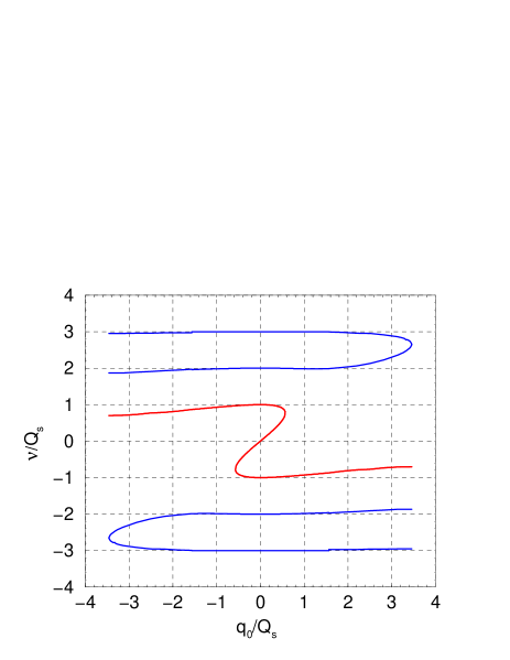
Figure 1: Real eigentunes of hollow bunch without chromaticity (exact solutions). There are complex roots at $|q_{0}|/Q_{s}>0.567$ (not shown).

Table 1: Threshold of different TMCI modes

Coalesced multipoles	(0-1)	(2-3)	(4-5)	(6-7)	(8-9)	(10-11)
$(q_{0})_{thresh}/Q_{s}$	0.5671	3.459	7.366	11.894	16.871	22.198

Hence the modes $|m|>1$ have a minor interest from point of view of the instability threshold. Therefore our goal should be an investigation of the lower modes presented by red line in Fig. 1, using realistic distributions and wake functions, with chromaticity and space charge taken into account.

IV Integral equations for multipoles

General solution of Eq. (8) can be presented as the Fourier series:

$$Y(A,\phi)=\sum_{m}Y_{m}(A)\exp(im\phi)$$ (17)

which is just expansion over the multipoles. Its substitution to Eq. (8) allows to get set of coupled integral equations for the functions $\,Y_{m}(A)$ SAH :

$$(\nu-mQ_{s})\,Y_{m}(A)=\;2\pi q_{0}\sum_{n}\int_{0}^{\infty}K_{m,n}(A,A^{\prime})Y_{n}(A^{\prime})\,F(A^{\prime})A^{\prime}\,dA^{\prime}$$ (18)

with the kernels

$$K_{m,n}(A,A^{\prime})=\frac{2}{\pi^{2}}\int_{-A}^{A}\exp(i\zeta_{\nu}\theta)\,\frac{T_{m}(\theta/A)\,d\theta}{\sqrt{A^{2}-\theta^{2}}}\int_{\theta_{A^{\prime}}}^{A^{\prime}}\!\exp(-i\zeta_{\nu}\theta^{\prime})\,\frac{T_{n}(\theta^{\prime}/A^{\prime})\,d\theta^{\prime}}{\sqrt{A^{\prime 2}-\theta^{\prime 2}}}$$ (19)

where $T_{m}(x)=\cos(m\arccos x)$ are Chebyshev polynomials,

$$\theta_{A^{\prime}}=\theta\;\;{\rm at}\;\,A^{{}^{\prime}2}>\theta^{2},\qquad{\rm and}\qquad\theta_{A^{\prime}}=A^{\prime}\times{\rm sign}(\theta)\;\;\,{\rm at}\;\;A^{{}^{\prime}2}<\theta^{2}.$$

The assumption $\zeta_{\nu}=0$ is used to start with but chromaticity will be added hereafter.

As it was established in previous section, the beam instability is governed mostly by the multipoles $m=0,\;\pm 1$, whereas other ones are of a minor importance. Corresponding kernels are:

$$K_{m,m}(A,A^{\prime})=K_{m,-m}(A,A^{\prime})=\delta_{m,0}$$ (20)

$$K_{0,\pm 1}(A,A^{\prime})=-K_{\pm 1,0}(A^{\prime},A)=\frac{2}{\pi^{2}A^{\prime}}\int_{-A}^{A}\sqrt{\frac{A^{\prime 2}-\theta_{A^{\prime}}^{2}}{A^{2}-\theta^{2}}}\,d\theta$$ (21)

(note that Eq. (20) is valid with any $m$ at $\zeta_{\nu}=0$). Therefore equations for three mentioned multipoles can be written in the form

$$\nu Y_{0}(A)=2\pi q_{0}\int_{0}^{\infty}\!\Big{\{}\,Y_{0}(A^{\prime})+K_{0,1}(A,A^{\prime})\big{[}Y_{-1}(A^{\prime})+Y_{1}(A^{\prime})\big{]}\Big{\}}F(A^{\prime})A^{\prime}\,dA^{\prime}$$ (22)

$$(\nu\mp Q_{s})Y_{\pm 1}(A)=\,-2\pi q_{0}\int_{0}^{\infty}K_{0,1}(A^{\prime},A)Y_{0}(A^{\prime})F(A^{\prime})A^{\prime}\,dA^{\prime}\;$$ (23)

Excluding $Y_{\pm 1}$ one can obtain the ordinary integral equation for the function $Y_{0}(A)$:

$$\nu Y_{0}(A)=2\pi q_{0}\int_{0}^{\infty}Y_{0}(A^{\prime})F(A^{\prime})A^{\prime}\,dA^{\prime}-\frac{8\pi^{2}q_{0}^{2}\nu}{\nu^{2}-Q_{s}^{2}}\int_{0}^{\infty}{\bf K}(A,A^{\prime})Y_{0}(A^{\prime})F(A^{\prime})A^{\prime}\,dA^{\prime}$$ (24)

with the kernel

$${\bf K}(A,A^{\prime})=\int_{0}^{\infty}\!\!K_{0,1}(A,X)K_{0,1}(A^{\prime},X)F(X)\,XdX$$ (25)

Multiplying Eq. (24) by $\,Y_{0}(A)F(A)A\,$ and integrating over $A$, one can get the simple equation for the eigentunes $\nu$

$$\frac{\nu-\bar{q}}{2}\biggl{(}\nu-\frac{Q_{s}^{2}}{\nu}\biggr{)}=-\alpha^{2}q_{0}^{2}$$ (26)

with the parameters which do not depend on $\,\nu$:

$$\bar{q}=\frac{2\pi q_{0}\,[\int_{0}^{\infty}Y_{0}(A)F(A)\,AdA]^{2}}{\int_{0}^{\infty}Y_{0}^{2}(A)F(A)A\,dA}$$ (27)

and

$$\alpha^{2}=\frac{4\pi^{2}\int_{0}^{\infty}\int_{0}^{\infty}{\bf K}(A,A^{\prime})\,Y_{0}(A)Y_{0}(A^{\prime})\,F(A)F(A^{\prime})\,AA^{\prime}\,dAdA^{\prime}}{\int_{0}^{\infty}Y_{0}^{2}(A)F(A)A\,dA}$$ (28)

These parameters are not too much sensitive to choice of the function $\,Y_{0}(A)$, so that some approximate solution of Eq. (24) can be used for the estimation. The function $\,Y_{0}=1\,$ is a simple and rather reasonable option because (i) it satisfies Eq. (24) without coupling presenting the lower radial mode at $q_{0}\ll 1$, (ii) and it is one of the exact solutions of Eq. (12) for hollow bunch with any $q_{0}$. True, higher radial modes are excluded from consideration by this choice. However, it does not matter in the case because it is known that these modes are much more stable SAH ; HAND .

With this choice, the relation $\,\bar{q}=q_{0}\,$ follows from Eq. (27), and Eq. (28) also obtains a compact form (see Appendix):

$$\alpha^{2}=\frac{8}{\pi}\int_{0}^{\infty}\!\!\!F(A)A^{3}\,dA\;\Big{[}\int_{0}^{\pi}\!\!\rho(A\cos\phi)\sin^{2}\phi\,d\phi\,\Big{]}^{2}$$ (29)

Table 2: Parameters $\,\alpha\,$ and TMCI threshold of different bunch shapes

	Hollow*	Hollow	Rectang	Parabol	Gauss
$\alpha$	N/A	0.4053	0.4082	0.4075	0.4020
$|q_{0}|_{\rm threshold}/Q_{s}$	0.5671	0.5689	0.5672	0.5676	0.5708

Results of calculated by this formula are collected in Table II for several distributions. Somewhat surprising fact is very slight dependence of the parameters on the bunch shape, even for so far apart models as the hollow and the Gaussian bunches. It is confirmed by Fig. 2 where solutions of Eq. (26) are plotted against the wake strength, and the images of different distributions are also indistinguishable. The data taken from Section III are also transferred in this graph being presented by the dark circles, and demonstrating absolute agreement of the results obtained by so different methods.

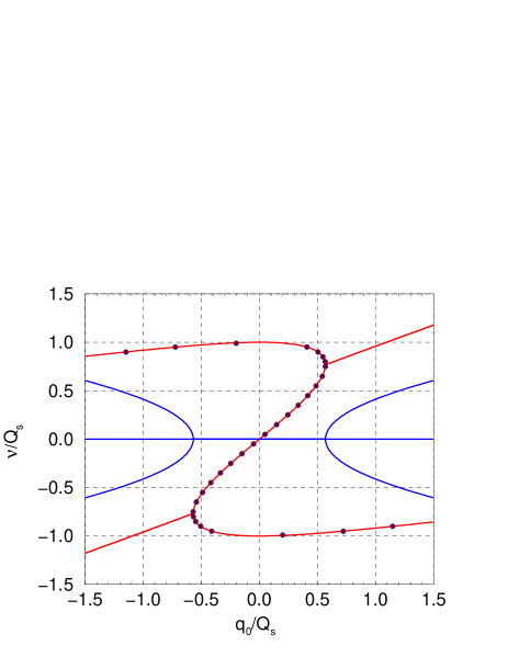
Figure 2: Eigentunes of hollow bunch without chromaticity (3-modes approximation). Red and blue curves present real and imaginary parts of the tune. Solid lines are obtained by solution of Eq. (25), and some data are transfered from Fig. 1 being presented by circles.

The eigentunes shown in Fig. 2 are real numbers at low wake. However, they obtain an imaginary addition (blue lines) at rather large $\,q_{0},$ which is the TMCI threshold in the case. Corresponding values are presented in the last line of Table II being about 0.57 in all the examples. In agreement with definition given by Eq. (7), it allows to represent the TMCI threshold in usual terms

$$\frac{r_{0}RN|W_{1}|}{8\beta\gamma Q_{0}Q_{s}}>0.57\pi\simeq 1.8$$ (30)

which expression almost does not depend the bunch shape. The result coincides very well with the known expressions KOH ; CHAO ; CHIN ; NG ; HAND .

V Three-mode model with chromaticity

As it has been shown in previous section, the function $\,Y_{0}=1\,$ is rather good approximation to describe the single bunch instability near threshold at zero chromaticity. Besides, the relation

$$Y_{\pm 1}(A)\propto A\int_{0}^{\pi}\rho(A\cos\phi)\sin^{2}\phi\,d\phi$$ (31)

follows from Eq. (21) and Eq. (23) in this approximation. Important thing is that the integral in this expression moderately depends on the amplitude at realistic distributions. For example, it does not depend at all for the rectangular bunch, and has a variation not more of 25% for the parabolic one. Therefore the approximation $Y_{\pm 1}\propto A$ looks rather reasonably for this case. It means that all above presented results could be obtained using the pattern solution

$$Y(A,\phi)=1+C_{\theta}\theta+C_{u}u$$ (32)

with indefinite constants $C_{\theta}$ and $C_{u}$. Confirmations of this statement will be furnished later. However, the main thing is that this model paves the way to extend the theory by including chromaticity, space charge, etc. Chromaticity is the fist point which will be applied in this section.

Substitution of Eq. (32) to Eq. (8) results in

$$\nu+(\nu C_{\theta}\!+\!iQ_{s}C_{u})\,\theta+(\nu C_{u}\!-\!iQ_{s}C_{\theta})\,u=2q_{0}\exp(i\zeta\theta)\int_{\theta}^{\infty}\!\!\!\!\rho(\theta^{\prime})(1\!+\!C_{\theta}\theta^{\prime})\exp(-i\zeta\theta^{\prime})\,d\theta^{\prime}\quad\;\;$$ (33)

The relation $\,C_{u}=iC_{\theta}Q_{s}/\nu\,$ follows from this immediately. Two more equations can be obtained by multiplication of Eq. (33) by $\rho(\theta)$ or $\rho(\theta)\theta$ with subsequent integration over $\;\theta$. Then, excluding parameter $C_{\theta}$, one can get required dispersion equation for the eigentunes $\nu$. It is represented below for the case $|\zeta\theta_{0}|<\sim 0.5$ which assumption allows to estimate effect of chromaticity without excessively bulky expressions:

$$\frac{\nu-q_{0}(1-i\alpha\chi)}{2}\left(\nu-\frac{Q_{s}^{2}}{\nu}-2i\beta q_{0}\chi\right)\simeq-q_{0}^{2}\left(\alpha-\frac{i\chi}{4}\right)^{2}$$ (34)

where $\chi=2\sqrt{2}\,\zeta_{\nu}\sigma_{\theta}$, and following designations are applied:

$$\sigma_{\theta}^{2}=\int_{-\infty}^{\infty}\rho(\theta)\,\theta^{2}d\theta,\;\hskip 88.20354pt$$ (35a)

$$\alpha=\frac{\sqrt{2}}{\sigma_{\theta}}\int_{-\infty}^{\infty}\rho(\theta)\,\theta d\theta\int_{0}^{\theta}\rho(\theta^{\prime})\,d\theta^{\prime},\quad\;$$ (35b)

$$\beta=\frac{1}{\sigma_{\theta}^{3}\sqrt{2}}\int_{-1}^{1}\rho(\theta)\,\theta d\theta\int_{0}^{\theta}\rho(\theta^{\prime})\,\theta^{\prime 2}d\theta^{\prime}$$ (35c)

Table 3: Dispersion equation parameters of different bunches

	Hollow	Boxcar	Parabolic	Gaussian
$\quad\sigma_{\theta}^{2}\quad$	$\qquad\theta_{0}^{2}/2\qquad$	$\quad\theta_{0}^{2}/3\qquad$	$\qquad\theta_{0}^{2}/5\qquad$	Any
$\alpha$	0.405	0.408	0.407	0.400
$\beta$	0.135	0.123	0.113	0.100

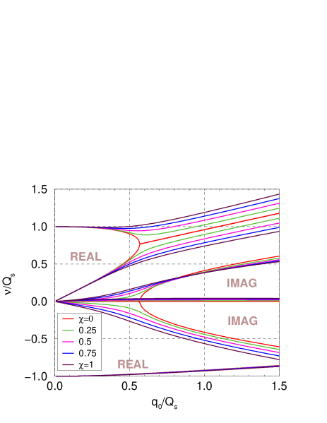
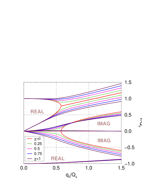
Figure 3: Eigentunes with chromaticity: left – hollow bunch, right – Gaussian distribution. All the curves are odd functions of the wake strength. Real parts do not depend on sign of chromaticity, imaginary parts change sign. Some curves are indistinguishable because the modes starting from the point $\nu=-Q_{s}$ almost do not depend on chromaticity.

Because $\sigma_{\theta}$ is rms bunch length, $\chi$ can be treated as betatron phase advance caused by chromaticity in the entire bunch (it is really true for the hollow bunch of length $\,2\theta_{0}\,$ when $\,\sigma_{\theta}=\theta_{0}/\sqrt{2}$). Other parameters are represented in Table III for several distributions. Comparison with Table II let us to conclude that Eq. (26) and (34) coincide not only formally but also actually at $\chi=0$, because the difference of coefficients $\alpha$ is negligible. It can be concluded as well that the dependence of the eigentunes on the bunch shape is very weak when the chromaticity is also included. The statement is confirmed by Fig. 3 where complex solutions of Eq. (34) are plotted against the wake strength at different chromaticity, for hollow and Gaussian bunches. Note that only positive wakes and chromaticities are presented in the graphs because all curves have following symmetry properties: (i) they are odd functions of $q_{0}/Q_{s}$; (ii) real parts of the tunes do not depend on sign of chromaticity; (iii) the imaginary additions reflect specularly with respect to the line $\nu=0$, when the chromaticity change sign. It is seen that the instability has no threshold with chromaticity, and TMCI appears against the head-tail background without a pronounced demarcation line. In particular, the head-tail and TMCI contributions are comparable at $\,|q_{0}|\simeq 0.7\,Q_{s}\,$ and $\,|\theta_{0}\zeta|\simeq 0.5$. It should be noted in addition that no sign of chromaticity can prevent instability of all bunch modes.

With accuracy of several percents, solutions of Eq. (34) at $\,q_{0}<Q_{s}\,$ can be presented in the form

$$\nu\;\simeq\;\frac{q_{0}+mQ_{s}-iq_{0}\chi(\alpha-\beta)}{2}\pm\sqrt{\biggl{(}\frac{q_{0}-mQ_{s}-iq_{0}\chi(\alpha+\beta)}{2}\biggr{)}^{2}-q_{0}^{2}\biggl{(}\alpha-\frac{i\chi}{4}\biggr{)}^{2}}$$ (36)

where $\,m=\pm 1$. In particular, it provides correct TMCI threshold without chromaticity, and leads to well known formulae for the head-tail modes at $\,q_{0}\ll Q_{s}$. In the last case the solutions for hollow bunch can be reduced to the form:

$$\nu_{m}=mQ_{s}+q_{0}\delta_{m,0}+\frac{8iq_{0}\theta_{0}\zeta_{\nu}}{\pi^{2}(4m^{2}-1)}$$ (37)

which expression is valid with any $\,m\,$ CHAO . Analyzing Table III, one can add that this result almost does not depend on the bunch shape, at least for lowest radial modes and multipoles.

VI Realistic bunch with arbitrary wake

It would be beyond reasons to treat rectangular wake as an exclusive case. On the contrary, Eq. (32) can be applied as an approximate solution of general Eq. (6) to look for the eigentunes of a bunch with arbitrary wake function. Subsequent transformations are described just after Eq. (32) and result in the dispersion equation like Eq. (34) or (26):

$$\frac{\nu-q_{ef}}{2}\left(\nu-\frac{Q_{s}^{2}}{\nu}-2\alpha_{2}q_{ef}\right)=-\alpha_{1}^{2}q_{ef}^{2}$$ (38)

with the coefficients

$$q_{ef}=2\int_{0}^{\infty}\tilde{q}(\theta)d\theta\;\int_{-\infty}^{\infty}\rho(\theta^{\prime}-\theta/2)\;\rho(\theta^{\prime}+\theta/2)\,d\theta^{\prime}\hskip 76.82243pt$$ (39a)

$$\alpha_{1}=\frac{1}{\sigma_{\theta}q_{ef}\sqrt{2}}\int_{0}^{\infty}\tilde{q}(\theta)\,\theta d\theta\times\int_{-\infty}^{\infty}\rho(\theta^{\prime}-\theta/2)\,\rho(\theta^{\prime}+\theta/2)\,d\theta^{\prime}\qquad$$ (39b)

$$\alpha_{2}=\frac{1}{\sigma_{\theta}^{2}q_{ef}}\int_{0}^{\infty}\tilde{q}(\theta)\,d\theta\int_{-\infty}^{\infty}\!\!\rho(\theta^{\prime}-\theta/2)\,\rho(\theta^{\prime}+\theta/2)\,(\theta^{\prime 2}-\theta^{2}/4)\,d\theta^{\prime}$$ (39c)

where $\sigma_{\theta}$ is rms bunch length given by Eq. (35a), and $\,\tilde{q}(\theta)=q(\theta)\exp(-i\zeta_{\nu}\theta)$. Approximate solutions of Eq. (38) can be presented in the form like Eq. (36):

$$\nu\simeq\frac{q_{ef}(1+\alpha_{2})+mQ_{s}}{2}\pm\sqrt{\biggl{[}\frac{q_{ef}(1-\alpha_{2})-mQ_{s}}{2}\biggr{]}^{2}\!\!\!-\alpha_{1}^{2}q_{ef}^{2}}$$ (40)

with $\,m=\pm 1$. Although parameter $\,\chi\,$ does not appear in the expression, chromaticity is still presented here being included in the functions $\,\tilde{q}(\theta)$ and $q_{\rm ef}$. However, next consideration will be restricted by the case of zero chromaticity: $\,\zeta_{\nu}=0,\;\tilde{q}(\theta)=q(\theta)$. Then $\alpha_{1,2}$ are real numbers, and the instability can appear only in the TMCI form with the threshold:

$$|q_{ef}|_{thresh}=\frac{Q_{s}}{1+2\alpha},\qquad\alpha=\alpha_{1}-\frac{\alpha_{2}}{2}$$ (41)

For Gaussian bunch with dispersion $\sigma_{\theta}$, used parameters obtain the forms

$$q_{ef}=\frac{1}{\sigma_{\theta}\sqrt{\pi}}\int_{0}^{\infty}\exp\biggl{(}-\frac{\theta^{2}}{4\sigma_{\theta}^{2}}\biggr{)}\,q(\theta)\,d\theta\hskip 79.66771pt$$ (42a)

$$\alpha_{1}=\frac{1}{2\sqrt{2\pi}\,\sigma_{\theta}^{2}q_{ef}}\int_{0}^{\infty}\exp\biggl{(}-\frac{\theta^{2}}{4\sigma_{\theta}^{2}}\biggr{)}\,q(\theta)\,\theta d\theta\hskip 45.5244pt$$ (42b)

$$\alpha_{2}=\frac{1}{4\sqrt{\pi}\,\sigma_{\theta}q_{ef}}\int_{0}^{\infty}\biggl{(}1-\frac{\theta^{2}}{2\sigma_{\theta}^{2}}\biggr{)}\exp\biggl{(}-\frac{\theta^{2}}{4\sigma_{\theta}^{2}}\biggr{)}\,q(\theta)\,d\theta$$ (42c)

Note that $\,q_{ef}=q_{0},\,\alpha_{1}=\alpha,\,\alpha_{2}=0\,$ at constant wake $\,q=q_{0}$. Two more examples are considered below.

VI.1 Short rectangular wake

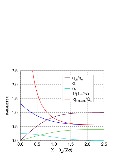
Figure 4: Parameters of Gaussian bunch with short rectangular wake. Brown line describes an effective weakening of the wake in a short bunch, red line represents TMCI threshold.

Gaussian bunch with a rectangular wake of restricted length $\theta_{w}$ is considered in this subsection as first example (similar wake can be created e.g. by a pair of strip-line BPM HAND ). Eq. (42) gives in this case

$$q_{ef}=q_{0}\,{\rm erf}(x),\qquad\alpha_{1}=\frac{1-\exp(-x^{2})}{\sqrt{2\pi}\,{\rm erf}\,(x)},\qquad\alpha_{2}=\frac{x\exp(-x^{2})}{2\sqrt{\pi}\,{\rm erf}\,(x)}$$ (43)

where $x=\theta_{w}/(2\sigma_{\theta})$. These functions are plotted in Fig. 4. Threshold value of $\,q_{0}\,$ is shown as well being determined with help of the expression

$$\frac{|q_{0}|_{thresh}}{Q_{s}}=\frac{1}{[1+2\alpha(x)]\,{\rm erf}\,(x)}$$ (44)

It is seen that a shortening of the wake results in a rise of the threshold which becomes especially noticeable at $\,\theta_{w}<\sim 2\sigma\,$.

VI.2 Resistive wake

Resistive wall impedance is the most general and important source of transverse instabilities in circular accelerators. Corresponding normalized wake function is

$$q(\theta)=\frac{q_{rw}}{\sqrt{\theta}},\qquad\quad{q_{rw}}=-\frac{r_{0}R^{2}N}{2\pi\beta\gamma Q_{0}b^{3}}\sqrt{\frac{c}{R\sigma_{c}}}$$ (45)

where $b$ is the beam pipe radius, and $\sigma_{c}$ is the pipe wall conductivity (see e.g. HAND ). With this wake, integrals in Eq. (42) are representable in terms of gamma functions:

$$q_{ef}=\frac{q_{rw}\,\Gamma(1/4)}{\sqrt{2\pi\sigma_{\theta}}}=\frac{1.4464\,q_{rw}}{\sqrt{\sigma_{\theta}}},\qquad\alpha_{1}=\frac{\Gamma(3/4)}{\sqrt{2}\,\Gamma(1/4)}=0.2390,\qquad\alpha_{2}=\frac{1}{8}$$ (46)

Threshold value of the effective and usual wakes can be found then with help of Eq. (41): $\;|q_{ef}|_{thresh}=0.739\,Q_{s},\;\;|q_{rw}|_{thresh}=0.511\,Q_{s}\sqrt{\sigma}_{\theta}.\;$ Therefore the resistive wall TMCI threshold in usual terms is

$$\frac{r_{0}R^{2}N_{thresh}}{2\pi\beta\gamma Q_{0}Q_{s}b^{3}}\sqrt{\frac{c}{\sigma_{c}\sigma_{z}}}=0.51$$ (47)

where standard rms bunch length $\,\sigma_{z}=\sigma_{\theta}R\,$ is used. However, it is necessary to take into account that Eq. (45) is valid only at $R\theta>\sim b/\gamma$ when the wake reaches a maximum. Therefore sufficient condition of applicability of Eq. (47) is $\sigma_{z}\gg b/\gamma$.

Another restriction comes from the fact that the resistive wake has a long and slowly decaying tail. Therefore it can impact not only next bunches but also itself by the succeeding turns. These multibunch/multiturn collective effects should be included in a comprehensive investigation of resistive wall instability. However, this point is beyond the scope of the paper where only single bunch effects are examined. Nevertheless it can be noted that presented results give a possibility to estimate a relative danger of the effects by a comparison of the contributed tune shifts. Indeed, TMCI of a single bunch appears at $\,|\nu|_{\rm TMCI}\simeq 0.77\,Q_{s}\,$ as it follows from Fig. 1-3, and corresponding bunch population is determined by Eq. (47). The collective modes i.e. long term tune shift with this intensity is B2

$$|\nu|_{\rm LONG}\simeq 0.51\,Q_{s}\sqrt{\frac{2\beta\sigma_{z}}{2\pi R|k-Q_{0}|}}\biggr{(}h-\frac{(2|k-Q_{0}|)^{3/2}}{h^{1/2}}\biggr{)}$$ (48)

where $h$ is number of bunches, and $k$ is the collective mode number (the mode can be unstable at $k>Q_{0}$). Taking $\,|k-Q_{0}|=0.25\,$ and $\,\beta=1\,$ as a typical example, we can compare these long term and TMCI effects as the ratio of corresponding tune shifts:

$$\biggl{|}\frac{\nu_{\rm LONG}}{\nu_{TMCI}}\biggr{|}\sim 2\,\biggr{(}h-\frac{0.35}{\sqrt{h}}\biggr{)}\sqrt{\frac{\sigma_{z}}{2\pi R}}$$ (49)

With great probability this value is $\,<1\,$ or even $\,\ll 1\,$ at $\,h=1$, that is the multiturn effect of a single bunch is typically small or even negligible in comparison with TMCI or head-tail instability. However, the collective effects are more dangerous in a multibunch machine with $\,h\gg 1,\;h\sigma_{z}\sim R$. Of course, more detailed analysis is required at intermediate cases.

VII Space charge effects

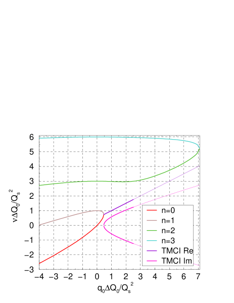
Figure 5: Eigentunes of a rectangular (“boxcar”) bunch with ultimate space charge $\Delta Q_{0}\gg Q_{s}$. The graph is taken from B1 ; $n=m(m+1)/2$.

Bunched beam instability with extremely large space charge $(\Delta Q\gg Q_{s})$ was considered in works BU ; B1 ; B2 . The most remarkable phenomenon is a pronounced asymmetry of the curves with respect to the wake sign which effect has been first shown in Ref. B1 . It is illustrated by Fig. 5 taken from the quoted article where a rectangular (“boxcar”) bunch with constant wake was explored at space charge betatron tune shift $\Delta Q_{0}\gg Q_{s}$. It is seen that TMCI appears only with the positive wake satisfying the instability condition

$$(q_{0})_{thresh}\simeq\frac{0.5\,Q_{s}^{2}}{\Delta Q_{0}}$$ (50)

which drastically differs from the conditions presented by Fig. 1-3, and Eq. (30) of this paper. It is needless to say that investigation of the effect at $\Delta Q_{0}\sim Q_{s}$ is the only way to resolve the problem by a joining of these conflicting pictures. It turns out that the 3-modes model described by Eq. (32) bridges these ultimate cases providing a general form of the lowers eigenmodes over a wide range of parameters.

It is easy to verify that substitution of Eq. (32) to general Eq. (6) results in

$$\nu+(\nu C_{\theta}\!+\!iQ_{s}C_{u})\,\theta+\big{\{}\big{[}\,(\Delta Q_{av}\rho(\theta)+\nu\big{]}C_{u}\!-\!iQ_{s}C_{\theta}]\big{\}}\,u$$

$$=\>2q_{0}\exp(i\zeta\theta)\int_{\theta}^{\infty}\rho(\theta^{\prime})(1+C_{\theta}\theta^{\prime})\exp(-i\zeta\theta^{\prime})\,d\theta^{\prime}$$ (51)

The only distinction of this expression from Eq. (33) without space charge is the addition proportional to $\Delta Q_{av}\rho(\theta)$. We consider in this section a rectangular bunch which density does not depend on longitudinal coordinate so that $Q_{av}\rho$ is the constant value $\,\Delta Q_{0}\,$ which coincides with incoherent space charge tune shift averaged over all transverse coordinates B2 . Therefore relation between coefficients of Eq. (51) obtains the form $\,C_{u}=iC_{\theta}Q_{s}/(\nu+\Delta Q_{0})\,$ instead of $\,C_{u}=iC_{\theta}Q_{s}/\nu$. As a result, all subsequent relations hold true with the replacement of $\,Q_{s}^{2}/\nu\,$ on $\,Q_{s}^{2}/(\nu+\Delta Q_{0})$. In particular, Eq. (34) with constant wake function and chromaticity obtains the form

$$\frac{\nu-q_{0}(1-i\alpha\chi)}{2}\left(\nu-\frac{Q_{s}^{2}}{\nu+\Delta Q_{0}}-2i\beta q_{0}\chi\right)\simeq-q_{0}^{2}\left(\alpha-\frac{i\chi}{4}\right)^{2}$$ (52)

In the “head-tail” limit, that is at $\,|q_{0}|\ll Q_{s}\,$, approximate solutions of the equation are

$$\nu_{0}=q_{0}(1-i\alpha\chi),\qquad\nu_{\pm 1}\simeq\pm\sqrt{Q_{s}^{2}+\frac{\Delta Q_{0}^{2}}{4}}-\frac{\Delta Q_{0}}{2}+i\beta q_{0}\chi$$ (53)

Thus space charge does not affect zero mode at all and does not change growth rate of the modes $\,m=\pm 1\,$ in this “head-tail” approximation.

Another situation arises at $\,q_{0}\sim Q_{s}\,$ or $\,q_{0}>Q_{s}\,$ where TMCI can arise. This case is illustrated by Fig. 6 where the eigentunes are plotted against the wake strength at different space charge, but without chromaticity. Effect of the wake sign is seen very clearly in this graph: space charge propels the TMCI threshold to the centerline at $q_{0}>0$, and away from it at $q_{0}<0$. Corresponding dependence is shown quantitatively in Fig. 7 where the thresholds are presented separately for positive and negative wakes and supplemented by appropriate analytical formulae. There is very good agreement of these results with Fig. 5. For example, TMCI threshold of positive wake is

$$(q_{0})_{thresh}\simeq\frac{0.57\,Q_{s}^{2}}{Q_{s}+\Delta Q_{0}}\rightarrow\frac{0.57\,Q_{s}^{2}}{\Delta Q_{0}}$$ (54)

what is very close to the estimation given by Fig. 5 and Eq. (50).

However, space charge tune shift raises the TMCI threshold of negative wakes. For example, Eq. (47) for resistive wall TMCI threshold obtains the form:

$$\frac{r_{0}R^{2}N_{thresh}}{2\pi\beta\gamma Q_{0}Q_{s}b^{3}}\sqrt{\frac{\Omega_{0}R}{\sigma_{c}\sigma_{z}}}\simeq 0.51\biggl{(}1+\frac{0.7\Delta Q_{0}}{Q_{s}}+\frac{0.3\Delta Q_{0}^{2}}{Q_{s}^{2}}\biggr{)}$$ (55)

Joint effect of space charge and chromaticity is illustrated by Fig. 8 where dependence of the eigentunes of rectangular bunch on the wake strength is presented at $\Delta Q_{0}=Q_{s}$ and various chromaticity.

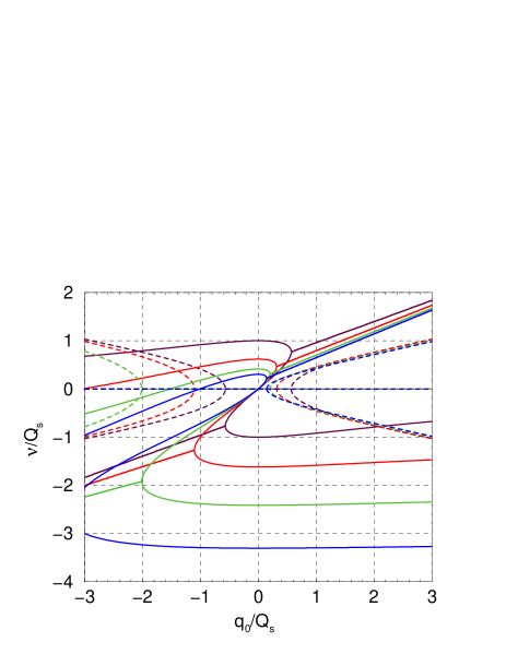
Figure 6: Eigentunes of rectangular bunch with space charge (chromaticity is turned off). Used ratios $\,\Delta Q_{0}/Q_{s}\,$ are: 0 (maroon), 1 (red), 2 (green), and 3 (blue). Solid/dashed lines represent real/imaginary parts of the tune.

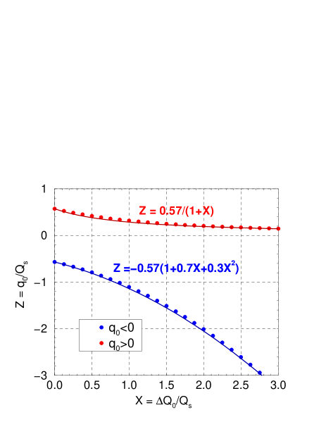
Figure 7: TMCI threshold of the rectangular bunch against the space charge tune shift. Positive and negative wakes are presented separately, no chromaticity.

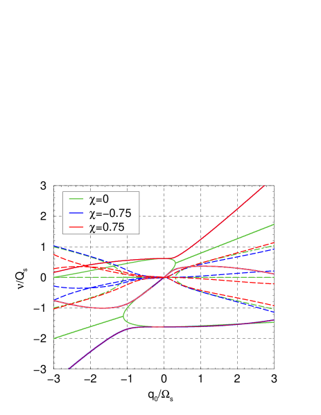
Figure 8: Eigentunes of rectangular bunch with $\Delta Q_{0}=Q_{s}$ and chromaticity. Solid/dashed lines represent real/imaginary parts of the tune. Some red and blue solid lines coalesce because real part of the tune is even function of chromaticity.

VII.1 Discussion

The most unstable TMCI mode with space charge was considered in Ref. BL where expansion of eigenfunctions in terms of azimuthal and radial modes has been applied. Fig. 1 of the paper gives an example of negative wake which is twice the size needed to produce instability without space charge: $W/|W_{\rm thresh}(0)|=-2$. The results depend on number of the basis modes which is characterized by the number $m_{\rm max}$. According them, the instability disappears at rather large $\Delta Q_{\rm sc}/Q_{s}$, and threshold values of this parameters are: 0.85 at $m_{\rm max}=1$ (3 multipoles), 0.5 at $m_{\rm max}=5$ or 10 (21 multipoles and up to 5 radial modes in the last case). My Eq. (52) provide reasonably close parameters of the threshold: $\Delta Q_{0}/Q_{s}=1$ at $q_{0}/Q_{s}=-1.14$ (point $X=1,\,Y=-1.14$ in Fig. 7).

However, there is a profound disagreement at the larger space charge tune shift. A monotonous behavior of the threshold follows from my paper, and this statement does not contradict Fig. 1 with $m_{\rm max}=1$ and 5. However, new region of instability at $\Delta Q>2.2$ is predicted by the figure with $m_{\rm max}=10$. This problem is pointed but not explained in BL (end of Sec.II).

Analytical and numerical investigation of the model with hollow bunch in square potential well is also performed in Ref. BL . Being compared with Fig. 1, the results agree with option $m_{\rm max}=1$ better than with multi-modes approach. At least, Fig. 13 obtained by numerical solution of differential equation demonstrates a monotonous behavior of the threshold, without additional instability regions at higher $\Delta Q_{0}$. However, analytical expression for $\Delta Q_{x}$ in page 10 gives a way of head-tail instability even without chromaticity and space charge. I guess this statement is in a conflict with commonly accepted point of view CHAO ; NG ; HAND . My Eq. (53) has another appearance and does not suffer from this shortcoming.

My results correlate well with the multi-particle simulations presented in Ref. BLA . For example, Fig. 1 of this paper resembles my Fig. 6 and allows to find TMCI thresholds of square bunch at $\Delta Q_{0}/Q_{s}=4$. According it, the relative wake strength is: $W_{\rm thresh}/|W_{0}|\simeq-9$ for negative wake, and 0.2 – 0.3 for positive one where $W_{0}$ is the threshold value for no space charge (it is difficult to get more exact numbers from the plot). In terms of my paper $W_{\rm thresh}/|W_{0}|=(q_{0})_{\rm thresh}/(0.57Q_{s})$ which value should be $-8.6$ or 0.2, according to my Fig. 7. Another example is provided by Fig. 3 BLA where threshold value of the wake is presented as a function of $\Delta Q/Q_{s}$. The curves for square bunch coincide with my Fig. 7 not only in shape but also quantitatively. Indeed, it follows from Fig. 3 that $W_{\rm thresh}/|W_{0}|\simeq-6$ at $\Delta Q_{0}/Q_{s}=3$. In terms of my paper, it means $q_{\rm thresh}/Q_{s}=-6\times 0.57\simeq-3.4$ while the value -3.3 follows from Fig.7. Positive wake thresholds are in a good consent as well being presented in these figures. However, the agreement is not so close for smooth bunch. According to Fig. 3 BLA , thresholds of the smooth and square bunches have a similar behavior at $\Delta Q_{\rm sc}/Q_{s}<3$. The similarity is especially obvious if the averaged across the bunch value is used as the argument ($\Delta Q_{0}=0.43\Delta Q_{\rm sc}$ for this distribution). However, the results come apart at larger tune shift because non-monotonous behavior of the smooth bunch is shown in Ref. BLA .

VIII Conclusion

The theory of a single bunch transverse instability is advanced in the paper by development of 3-modes model for the most unstable bunch modes. The dispersion equation is presented in form of 3rd order algebraic equation which includes chromaticity and space charge, and can be used with any bunch shape and wake field form.

The known TMCI and head-tail instability appear in the theory as the limiting cases. It is shown that a distinct boundary between them exists only at zero chromaticity representing the TMCI threshold in the case. Generally, the TMCI appears more or less smoothly against the head-tail background without a pronounced demarcation line.

The results depend very slightly on the bunch shape so that simple bunch models can be successfully used to analyze the stability limits. For example, difference of the TMCI thresholds is less of 1% for so far models as hollow and Gaussian bunches, if they have the same rms length and space charge is negligible.

In contrast with this, the tunes essentially depend on the wake form. Several cases are investigated in the paper including arbitrary rectangular and resistive wall wakes. Comparison of the single bunch and multibunch/multiturn effects is realized in the last case.

Space charge tune shift is included in the consideration at arbitrary relation of the shift to the synchrotron tune. It is shown that the space charge effect depends on the wake sign: it increases the instability threshold if the wake is negative, and decreases it at positive wakes. Simple analytical formulae are presented for the instability threshold and growth rate. They coincide well with the known expressions in the limiting cases though generally there are some divergences which are discussed in the paper.

IX Appendix: Derivation of Eq. (29)

It follows from Eq. (25) and (28) at $Y_{0}=1$,

$$\alpha^{2}=8\pi^{3}\int_{0}^{\infty}F(A)\,AdA\,\biggl{[}\int_{0}^{\infty}K_{0,1}(A^{\prime},A)F(A^{\prime})A^{\prime}\,dA^{\prime}\,\biggr{]}^{2}$$

The substitution of $K_{0,1}$ from Eq. (21) results in

$$\alpha^{2}=\frac{128}{\pi}\int_{0}^{\infty}F(A)\,\frac{dA}{A}\biggl{[}\,\int_{0}^{\infty}F(A^{\prime})A^{\prime}dA^{\prime}\int_{0}^{A^{\prime}}\sqrt{\frac{A^{2}-\theta_{A}^{2}}{A^{\prime 2}-\theta^{2}}}\,d\theta\,\biggr{]}^{2}$$

where $\,\theta_{A}={\rm min}\{\theta,A$}. Changing sequence of the integrals obtain

$$\alpha^{2}=\frac{128}{\pi}\int_{0}^{\infty}F(A)\,\frac{dA}{A}\biggl{[}\,\int_{0}^{A}\sqrt{A^{2}-\theta^{2}}\,d\theta\int_{\theta}^{\infty}\frac{F(A^{\prime})A^{\prime}\,dA^{\prime}}{\sqrt{A^{\prime 2}-\theta^{2}}}\,\biggr{]}^{2}$$

The last integral is $\rho(\theta)/2$ so the expression is reducible in the form

$$\alpha^{2}=\frac{8}{\pi}\int_{0}^{\infty}F(A)A^{3}\,dA\biggl{[}\,\int_{-1}^{1}\rho(A\xi)\sqrt{1-\xi^{2}}\,d\xi\,\biggr{]}^{2}$$

which can be transformed in Eq. (29) by the substitution $\xi=\cos\phi$.

References

- (1) C. Pellegrini, Nuovo Cimento A64, 447 (1969).
- (2) M. Sands, SLAC TN-69-8 (1969).
- (3) F. Sacherer, CERN-SI-BR-72-5 (1972).
- (4) R. Kohaupt, in Proceeding of the XI International Conference on High Energy Accelerators, p. 562, Geneva (1980).
- (5) G. Besnier, D. Brandt, and B. Zotter, CERN/LEP-TH/84-11 (1984) Part. Accel. 17, 51-77 (1985)
- (6) Y. H. Chin, CERN/SPS/85-2, (1985).
- (7) A. W. Chao “Physics of Collective Beam Instabilities in High Energy Accelerators”, Wiley, 1993.
- (8) K. Y. Ng “Physics of Intensity Dependent Beam Instabilities”, Fermilab-FN-07-13 (2002).
- (9) M. Blaskiewicz, Phys. Rev. ST Accel. Beams 1,044201 (1998).
- (10) A. Burov, Phys. Rev. ST Accel. Beams 12,044202 (2009).
- (11) V. Balbekov, Phys. Rev. ST Accel. Beams 14,094401 (2011).
- (12) V. Balbekov, Phys. Rev. ST Accel. Beams 15,054403 (2012).
- (13) V.V.Danilov and E.A.Perevedentsev, in Proceeding of the 15 International Conference on High Energy Accelerators, p. 1163, Hamburg. CERN SL/92-57 (1992).
- (14) “Handbook of Accelerator Physics and Engineering”, edited by A.Chao and M. Tigner, World Scientific (1998), p. 204-208.
- (15) H. G. Hereward, CERN MPS/Int. DL-64-8 (1964).
-
(16)
M. Blaskiewicz, Proc. of IPAC2012, p. 3165 New Orleans, 2012.
http://accelconf.web.cern.ch/accelconf/ipac2012/papers/weppr097.pdf