Bayesian Budget Feasibility with Posted Pricing

Abstract

We consider the problem of budget feasible mechanism design proposed by Singer, (2010), but in a Bayesian setting. A principal has a public value for hiring a subset of the agents and a budget, while the agents have private costs for being hired. We consider both additive and submodular value functions of the principal. We show that there are simple, practical, ex post budget balanced posted pricing mechanisms that approximate the value obtained by the Bayesian optimal mechanism that is budget balanced only in expectation. A main motivating application for this work is crowdsourcing, e.g., on Mechanical Turk, where workers are drawn from a large population and posted pricing is standard. Our analysis methods relate to contention resolution schemes in submodular optimization of Vondrák et al., (2011) and the correlation gap analysis of Yan, (2011).

1 Introduction

Consider the problem of hiring workers to complete complex tasks on crowdsourcing platforms such as Mechanical Turk. A principal must select a set of participants, henceforth agents, whose contributions will be aggregated to complete the task. The principal’s value for the task is a function of the set of participants selected and the principal’s budget limits the total payments to participants. We assume that the principal’s value is submodular, i.e., it exhibits diminishing returns to recruiting additional participants. The participants have a private cost for participating and will choose to participate strategically to optimize their payments received relative to this cost. The principal seeks a budget feasible mechanism for selecting participants so as to maximize the value of the completed task.

The literature on budget feasible mechanism design initiated by Singer, (2010) studies this problem; however, it primarily considers sealed-bid mechanisms which do not tend to be seen on crowdsourcing platforms like Mechanical Turk. Instead, these platforms use posted pricing mechanisms. We follow a traditional economics approach to this problem where agents’ costs are drawn from a common prior distribution and a mechanism is sought to optimize the principal’s value function in expectation. Note that this approach is especially relevant to the principal’s problem as the workers on crowdsourcing platforms are drawn from a large population of available workers. We show that posted pricing mechanisms give a good approximation to the optimal sealed-bid mechanism. Additionally, we give efficient algorithms for calculating the appropriate prices. In comparison to other work in optimization of prices in crowdsourcing, our work focuses on the use of prices to control participation and not the level of effort of participants. Controlling the level of effort of participants was studied in online behavioral experiments by Ho et al., (2015), theoretically for crowdsourcing contests by Chawla et al., (2012), and for user generated content by Immorlica et al., (2015).

Overview of Approach.

Our approach follows similarly to that of Alaei, (2014) and Yan, (2011). The starting point for our analysis is an upper bound on the performance of the optimal sealed bid mechanism that relaxes the ex post budget constraint on the mechanism to hold ex ante, i.e., in expectation over the private costs of the agents. Via this ex ante relaxation and the Myerson, (1981) theory of virtual values, we construct a posted price mechanism that is budget feasible in expectation and a $1-1/e$ approximation to the optimal ex ante mechanism when the principal’s value function exhibits decreasing returns, i.e., is submodular. For the special case where the principal’s value function is additive, this posted pricing is optimal (for the ex ante relaxation).

We then consider posting the prices from the solution to the ex ante relaxation until the budget runs out. The resulting mechanism is ex post budget feasible, but suffers a loss in performance because the budget may run out early. The main technical contribution of this work is to show that the performance of such a price posting mechanism compares favorably to the optimal sealed-bid mechanism. Previous work in mechanism design gives techniques which are now well understood to satisfy ex post allocation constraints. Ex post payment constraints require different techniques and our analyses follow two basic approaches that combine optimization and mechanism design concepts. To analyze the performance of the posted pricing under any arrival order of the agents, we solve the ex ante relaxation with a slightly smaller budget and then, using results from the Vondrák et al., (2011) analysis of contention resolution schemes, show that it is unlikely for the original ex post budget constraint to bind. Alternatively, we obtain better bounds for additive value functions and when the order of agent arrivals can be specified by the mechanism via the correlation gap approach of Yan, (2011). As a corollary, we obtain new correlation gap results for integral and fractional knapsack set functions. Moreover, when the environment is symmetric (both in distribution of agent costs and the principal’s value function), the submodular case can be reduced to the additive case.

The prices identified above can be computed or approximately computed in polynomial time. In particular, for submodular value functions, we reduce the problem of finding the prices to the well-known greedy algorithm for submodular optimization. The identified prices approximate the optimal prices with relative loss in the value function that is within a factor of $1-1/e$. For additive value functions, the optimization problem simplifies to a monopoly pricing problem of classic microeconomics. Similarly to the Myerson and Satterthwaite, (1983) treatment of welfare maximization subject to budget balance in a buyer–seller exchange, optimization in this context is based on Lagrangian virtual surplus. These optimal prices can be approximated arbitrarily precisely by solving this problem on a discretized instance.

Related work.

The prior literature on budget feasibility primarily considers a worst-case design and analysis framework that compares the performance of the designed mechanism to the first-best outcome, i.e., the one that could be obtained if the agents’ costs were public. See Singer, (2010), Bei et al., (2012), Badanidiyuru et al., (2012), and Anari et al., (2014). Our analysis compares the designed mechanism, in expectation for the known prior distribution, to the second-best outcome, i.e., the one obtained by the Bayesian optimal mechanism.

The following results are for prior-free mechanisms in comparison to the first-best outcome. Singer, (2010) obtained a randomized truthful budget feasible mechanism with a constant factor approximation for submodular value functions, Chen et al., (2011) then improved the analysis of this mechanism to a 0.13 approximation. In the Bayesian setting, Bei et al., (2012) obtained a constant approximation for subadditive functions. More recently, Anari et al., (2014) obtained better bounds by considering large markets, which we also consider in this paper. Finally, Badanidiyuru et al., (2012) also considered posted pricing mechanisms but when the agents arrive online. They obtained a constant approximation for the class of symmetric submodular functions. They also obtained a $O(\log n)$ mechanism for the case of submodular functions. In comparison to this last paper, we give much better bounds when the prior distribution on costs is known.

The starting point for our analysis is the solution to the relaxed problem of budget balance in expectation, i.e., ex ante. In the additive case, this problem was recently studied by Ensthaler and Giebe, (2014). They show that posted pricing mechanisms solve the relaxed problem and remark that the same performance can be obtained with ex post budget balance, but at the expense of relaxing ex post individual rationality (for the bidders) and not with a posted pricing. This latter observation follows, for example, by applying a general construction of Esö and Futo, (1999). Our analysis of the relaxed problem gives a much simpler proof of their main theorem.

Budget feasibility has also been studied in the context of crowdsourcing. Among that line of work, the model considered in Anari et al., (2014) is the closest to ours, and will be compared in detail below. Singla and Krause, (2013) and Singer and Mittal, (2013) consider the special case of our model where the principal’s value function is the number of tasks performed. The former studies posted pricing for agents with i.i.d. costs from an unknown distribution, while the latter studies sealed bid mechanisms without a prior.

Our results.

Value Function	Mechanism Family	Ex Post Constraint Approach	General Result	Large Markets
Additive	Sequential Posted Pricing	Correlation Gap	$(1-\frac{1}{\sqrt{2\pi k}})(1-\frac{1}{k})$	$1$
Symmetric Submodular	Oblivious Posted Pricing	Correlation Gap	$(1-\frac{1}{\sqrt{2\pi k}})(1-\frac{1}{k})$	$1$
Submodular (computational)	Oblivious Posted Pricing	Contention Resolution	$(1-\frac{1}{e})^{2}(1-\epsilon)(1-e^{-\epsilon^{2}(1-\epsilon)k/12})$	$(1-\frac{1}{e})^{2}\approx 0.40$
Submodular (non-computational)	Oblivious Posted Pricing	Contention Resolution	$(1-\frac{1}{e})(1-\epsilon)(1-e^{-\epsilon^{2}(1-\epsilon)k/12})$	$1-\frac{1}{e}\approx 0.63$

Figure 1: Our results are approximations to the Bayesian optimal mechanism. Bounds are parameterized by the market size $k$, a lower bound on the number of agents that can be simultaneously selected with the given budget (see Definition 4). In large markets, $k$ grows large. The given results with the contention resolution approach require $k\geq 4$ and $\epsilon\in(2/k,1/2)$, a result for $k<4$ is mentioned in Section 4.. For the symmetric submodular results, we also assume symmetric distributions on costs. Our computational results also have an additional $o(1)$ loss due to discretization.

Our results are summarized in Figure 1. We consider two main classes of valuation functions, additive and submodular. We use two different methods to satisfy the ex post payment constraint, one is based on contention resolution schemes and the other on correlation gap. Contention resolution schemes give an oblivious posted price mechanism, i.e., one that obtains its proven bound under any arrival order of the agents. The correlation gap approach, for the case where the principal has an additive value function, gives a sequential posted price mechanism. Such a mechanism is specified by an ordering on agents and take-it-or-leave-it prices to offer each agent. As a special case, we consider symmetric environments where both the value function and the distribution is symmetric.

Our results can most directly be compared to those of Anari et al., (2014), but with the following caveats. Their results are for sealed bid mechanisms while ours are for posted pricings; their mechanism is prior-free while ours is parameterized by the prior distribution on agent costs; their results compare performance to the first-best outcome, i.e., without incentive constraints, while ours compare to the second-best outcome, i.e., that of the Bayesian optimal mechanism (with incentive constraints). They obtain approximation ratios of $1-1/e$, $1/3$ and $1/2$ in large markets respectively for additive, submodular (computational), and submodular (non-computational) value functions. Moreover, they show that no truthful mechanism can achieve an approximation ratio better than $1-1/e$ with respect to the first-best outcome for additive value functions.

Discussion about posted pricing mechanisms and benchmarks.

Following a line of literature in mechanism design that was initiated by Chawla et al., (2010), the goal of this work is to show that there exists simple posted pricing mechanisms that approximate the optimal sealed-bid mechanism. Two quantities of interest therefore need to be separated. The first is the cost of incentive compatibility in budget feasible settings, i.e., the gap between the first-best and second-best benchmarks. The second is the cost of simplicity, i.e., the loss of a posted pricing mechanism compared to the Bayesian optimal mechanism. Prior work with comparisons to a first-best benchmark has approximations that are a combination of both of these quantities. Our comparison to the second-best outcome isolates the loss from a simple decentralized pricing over the optimal centralized mechanism as the quantity of interest.

Paper Organization.

We start with preliminaries in Section 2 to introduce the model and different concepts used in this paper. We then describe posted price mechanisms for the ex ante relaxation, where the budget holds in expectation, in Section 3. We explain how to go from an ex ante posted price mechanism to an ex post posted price mechanism using two different methods, one inspired by contention resolution schemes in Section 4 and another based on a correlation gap analysis in Section 5. We tackle the computation issues of finding a good ex ante mechanism in Section 6. In Section 7, we study symmetric environments. Up to Section 7, cost distributions are assumed to be regular and Section 8 considers the case where some distributions might be irregular. Throughout the paper, we assume that the principal’s valuation function is monotone and submodular.

2 Preliminaries

There are $n$ agents $N=\{1,\ldots,n\}$. Agent $i$ has a private cost $c_{i}$ for providing a service that is drawn from a distribution $F_{i}$ (denoting the cumulative distribution function) with density $f_{i}$. Indicator variable $x_{i}$ denotes whether or not $i$ provides service and $p_{i}$ denotes the payment $i$ receives. Agent $i$ aims to optimize her utility given by $p_{i}-c_{i}x_{i}$. The cost profile is denoted $\boldsymbol{c}=(c_{1},\ldots,c_{n})$; the joint distribution on costs is the product distribution $\boldsymbol{F}=F_{1}\times\cdots\times F_{n}$; the payment profile is denoted $\boldsymbol{p}=(p_{1},\ldots,p_{n})$; and the allocation profile is denoted $\boldsymbol{x}=(x_{1},\ldots,x_{n})$.

The principal has a value function $v:\{0,1\}^{n}\to{\mathbb{R}}_{+}$. For allocation profile $\boldsymbol{x}\in\{0,1\}^{n}$ or set of agents $S=\{i:x_{i}=1\}$ who provide service, the value to the principal is $v(\boldsymbol{x})=v(S)$. The principal has a budget $B$ and requires the payments to the agents not to exceed the budget, i.e., $\sum_{i}p_{i}\leq B$. The following mathematical program captures the principal’s objective.

$$\max_{\boldsymbol{x},\boldsymbol{p}}\ \text{\bf E}_{\boldsymbol{c}}\!\left[v(\boldsymbol{x}(\boldsymbol{c}))\right]$$ (1)

s.t. $$\sum\nolimits_{i}p_{i}(\boldsymbol{c})\leq B\hskip 14.22636pt\forall\boldsymbol{c},$$

$$\boldsymbol{x}(\cdot) \boldsymbol{p}(\cdot)$$ and are incentive compatible.

We consider only mechanisms that are incentive compatible. A mechanism is incentive compatible (IC), if truthful reporting of the agents is a dominant strategy equilibrium. We will consider the budget constraint both ex ante, i.e., in expectation over realizations of agents’ costs and random choices of the mechanism, and ex post, i.e., the payments to the agents never exceed the budget. The main goal of this paper is to approximate the optimal ex ante budget feasible mechanism with an ex post budget feasible posted pricing mechanism. Posted pricing mechanisms are trivially incentive compatible.

Definition 1.

The posted pricing $(\hat{\boldsymbol{c}},\boldsymbol{\sigma})$, for prices $\hat{\boldsymbol{c}}$ and ordering on agents $\boldsymbol{\sigma}$, is:

1. The remaining budget is initially $B$.

2. The agents arrive in order $\boldsymbol{\sigma}$.

3. If agent $i$ arrives with cost $c_{i}$ below her offered price $\hat{c}_{i}$ which is below the remaining budget, then select this agent for service, pay her $\hat{c}_{i}$, and deduct $\hat{c}_{i}$ from the remaining budget. Otherwise, discard this agent.

For (implicit) distribution on costs $\boldsymbol{F}$, we can equivalently specify a posted pricing $(\hat{\boldsymbol{c}},\boldsymbol{\sigma})$ as $(\hat{\boldsymbol{q}},\boldsymbol{\sigma})$ where $\hat{q}_{i}=F_{i}(\hat{c}_{i})$ is the marginal probability that agent $i$ with cost $c_{i}\sim F_{i}$ would accept the price $\hat{c}_{i}$.

Note that the prices $\hat{\boldsymbol{c}}$ are non-adaptive, i.e., fixed before the agents arrive. We consider posted pricing mechanisms under two different models for agent arrival. In the sequential posted pricing model, the ordering $\boldsymbol{\sigma}$ can be fixed in advance by the mechanism and, without computational considerations, our analysis is for the best case ordering of the prices. In the oblivious posted pricing model, the ordering $\boldsymbol{\sigma}$ is unconstrained and our analysis is worst case with respect to this ordering. An oblivious posted pricing is denoted $\hat{\boldsymbol{c}}$. We compare our mechanisms to an ex ante posted pricing $\hat{\boldsymbol{c}}$ where the budget constraint holds in expectation, i.e., $\sum_{i}\hat{c}_{i}\,\hat{q}_{i}\leq B$. The value of an ex ante posted pricing is $\text{\bf E}_{S\sim\hat{\boldsymbol{q}}}\!\left[v(S)\right]$ where $S\sim\hat{\boldsymbol{q}}$ adds each agent $i$ to $S$ independently with probability $\hat{q}_{i}$.

The paper focuses on value functions that are monotone and submodular (Definition 2). An important special case, which we will treat separately, is that of additive value functions where each agent has a value $v_{i}$ and the value function is $v(S)=\sum_{i\in S}v_{i}$.

Definition 2.

A set function $v:\{0,1\}^{n}\to{\mathbb{R}}_{+}$ is monotone submodular if

• (monotonicity) $v(T)\leq v(S)$ for all $T\subset S$, and

• (submodularity) for all $T\subset S$ the marginal contribution of $i\not\in S$ to $T$ is at least its marginal contribution to $S$. In other words,

  $$v(T\cup\{i\})-v(T)\geq v(S\cup\{i\})-v(S).$$

Our analysis is based on the relationship between a set function and two standard extensions of a set functions from the domain $\{0,1\}^{n}$ to the domain $[0,1]^{n}$. For submodular set functions, these extensions were studied by Calinescu et al., (2007) and Agrawal et al., (2010).

Definition 3.

Given a set function $v:\{0,1\}^{n}\to{\mathbb{R}}_{+}$,

• its concave closure $V^{+}(\cdot)$ (a.k.a., correlated value) is the smallest concave function that upper bounds the set function. Alternatively, $V^{+}(\hat{\boldsymbol{q}})=\max_{{\cal D}}\text{\bf E}_{S\sim{\cal D}}\!\left[v(S)\right]$ with the maximization taken over all distributions ${\cal D}$ with marginal probabilities $\hat{\boldsymbol{q}}=(\hat{q}_{1},\ldots,\hat{q}_{n})$; and

• its multilinear extension $V(\cdot)$ (a.k.a., independent value) is the expected value of the set function when each element $i$ is drawn independently with marginal probability $\hat{q}_{i}$. In other words, $V(\hat{\boldsymbol{q}})=\text{\bf E}_{S\sim\hat{\boldsymbol{q}}}\!\left[v(S)\right]$.

For any set function, the concave closure is clearly an upper bound on the multilinear extension. For submodular functions the inequality approximately holds in the opposite direction as well. By the interpretation of the multilinear extension as the expected value of the set function for independent distribution and the concave closure as the expected value of the set function for correlated distributions, their worst case ratio over marginal probabilities $\hat{\boldsymbol{q}}$ is known as the correlation gap (Agrawal et al.,, 2010).

Theorem 1 (Calinescu et al.,, 2007, Agrawal et al.,, 2010).

For monotone submodular set function $v(\cdot)$, the correlation gap is

$$\min_{\hat{\boldsymbol{q}}}\frac{V(\hat{\boldsymbol{q}})}{V^{+}(\hat{\boldsymbol{q}})}\leq 1-1/e.$$

Theorem 2 (Yan,, 2011).

For a $k$-highest-value-elements set function $v(\cdot)$, which is additive with value $v_{i}$ for element $i$ up to a capacity of at most $k$ elements, the correlation gap is

$$\min_{\hat{\boldsymbol{q}}}\frac{V(\hat{\boldsymbol{q}})}{V^{+}(\hat{\boldsymbol{q}})}\leq 1-1/\sqrt{2\pi k}.$$

Our analysis is parameterized by a measure of the size of the market. This notion of market size is standard in the literature, e.g., see Bei et al., (2012) and Anari et al., (2014). A large market analysis considers the market size in the limit. Although large markets are described as an assumption by Anari et al., (2014), the market size $k$ is a parameter in our analysis and we obtain results for any market size.

Definition 4.

A market is $k$-large for prices $\hat{\boldsymbol{c}}$ and budget $B$ if $B/\hat{c}_{i}\geq k$ for all agents $i$.

Note that the market size depends on prices and therefore on the mechanism, which is inherent to our analysis. These prices can trivially be upper bounded by the maximum cost that can be drawn from the distributions.

3 The Ex Ante Budget Feasible and Concave Closure Relaxations

In this section we relax the objective function and the budget constraint to make the problem more amenable to optimization. We first relax the budget constraint so that it only holds in expectation, making it an ex ante feasibility constraint. We then upper bound the value function by its concave closure. With an ex ante feasibility constraint, the objective is to optimize the following ex ante program over allocation rule $\boldsymbol{x}(\cdot)$ and payment rule $\boldsymbol{p}(\cdot)$ with $\boldsymbol{c}\sim\boldsymbol{F}$.

$$\max_{\boldsymbol{x},\boldsymbol{p}}\ \text{\bf E}_{\boldsymbol{c}}\!\left[v(\boldsymbol{x}(\boldsymbol{c}))\right]$$ (2)

s.t. $$\sum\nolimits_{i}\text{\bf E}_{\boldsymbol{c}}\!\left[p_{i}(\boldsymbol{c})\right]\leq B,$$

$$\boldsymbol{x}(\cdot) \boldsymbol{p}(\cdot)$$ and are IC.

When payments are part of the principal’s objective or constraints, the Bayesian mechanism design problem will typically rely on the Myerson, (1981) theory of virtual values or, in our case where the agents are sellers, virtual costs. The virtual cost of agent $i$ with cost $c_{i}$ drawn from distribution $F_{i}$ is $\phi_{i}(c_{i})=c_{i}+\frac{F_{i}(c_{i})}{f_{i}(c_{i})}$. The virtual surplus of an agent $i$ with virtual cost $\phi_{i}(c_{i})$ and allocation indicator $x_{i}$ is $\phi_{i}(c_{i})\,x_{i}$.

Lemma (Myerson and Satterthwaite,, 1983).

In any incentive compatible mechanism, any agent $i$’s expected payment is equal to her expected virtual surplus, i.e., for $\boldsymbol{c}\sim\boldsymbol{F}$,

$$\text{\bf E}_{\boldsymbol{c}}\!\left[p_{i}(\boldsymbol{c})\right]=\text{\bf E}_{\boldsymbol{c}}\!\left[\phi_{i}(\boldsymbol{c})\,x_{i}(\boldsymbol{c})\right].$$

The definition of virtual costs and Lemma 3 allows the ex ante program (2) to be rewritten in terms of the allocation rule only. To do so, we invoke the following characterization of incentive compatible mechanisms of Myerson, (1981).

Lemma (Myerson,, 1981).

There exists an incentive compatible mechanism with allocation rule $\boldsymbol{x}(\cdot)$ if and only if $\boldsymbol{x}(\cdot)$ is monotone in the cost of any agent.

We now rewrite the optimization program (2) by substituting in virtual costs for payments to obtain the following virtual surplus program,

$$\max_{\boldsymbol{x}}\ \text{\bf E}_{\boldsymbol{c}}\!\left[v(\boldsymbol{x}(\boldsymbol{c}))\right]$$ (3)

s.t. $$\sum\nolimits_{i}\text{\bf E}_{\boldsymbol{c}}\!\left[\phi_{i}(\boldsymbol{c})\,x_{i}(\boldsymbol{c})\right]\leq B,$$

$$\boldsymbol{x}(\cdot)\text{ is monotone in the cost of any agent.}$$

For the general case of submodular value functions, the expected value of the set function $v(\cdot)$ is upper bounded by its concave closure (Definition 3) as follows. The allocation rule $\boldsymbol{x}(\cdot)$ that optimizes this virtual surplus program induces, for $\boldsymbol{c}\sim\boldsymbol{F}$, a distribution over sets of winning agents. Denote this distribution by ${\cal D}$ and denote by $\hat{\boldsymbol{q}}$ the profile of marginal probabilities, i.e., with $\hat{q}_{i}=\text{\bf Pr}_{S\sim{\cal D}}\!\left[i\in S\right]$. By the definition of the concave closure of the set function $v(\cdot)$, $\text{\bf E}_{\boldsymbol{c}}\!\left[v(\boldsymbol{x}(\boldsymbol{c}))\right]=\text{\bf E}_{S\sim{\cal D}}\!\left[v(S)\right]\leq V^{+}(\hat{\boldsymbol{q}})$.

The payment to an agent is lower bounded by the payment from price posting. As above, the optimal mechanism selects agent $i$ with probability $\hat{q}_{i}$. When virtual costs are monotonically increasing, i.e., in the case of regular distributions, the expected payment to an agent $i$ selected with probability $\hat{q}_{i}$ is minimized if agent $i$ is served if and only if $c_{i}\leq F_{i}^{-1}(\hat{q}_{i})$ by Lemma 3 since these costs minimize $\phi_{i}(\boldsymbol{c})$. Thus, the mechanism that minimizes expected payments and serves each agent $i$ with probability $\hat{q}_{i}$ is the mechanism that posts price $\hat{c}_{i}=F_{i}^{-1}(\hat{q}_{i})$ to each agent $i$.

Lemma .

For any agent with cost drawn from regular distribution $F_{i}$ and any incentive compatible mechanism that selects agent $i$ with probability $\hat{q}_{i}$, the expected payment of agent $i$ is at least $\hat{q}_{i}\hat{c}_{i}$ where $\hat{c}_{i}=F_{i}^{-1}(\hat{q}_{i})$.

Combining the relaxation of the value function and the relaxation of the payments we obtain the following concave closure program,

$$\max_{\boldsymbol{q}}\ V^{+}(\boldsymbol{q})$$ (4)

s.t. $$\sum\nolimits_{i}q_{i}F_{i}^{-1}(q_{i})\leq B.$$

Lemma .

Let $\hat{\boldsymbol{q}}^{+}$ be the optimal solution to the concave closure program (4), then $V^{+}(\hat{\boldsymbol{q}}^{+})$ upper bounds the performance of the optimal ex ante mechanism in the case of regular cost distributions.

Posted price mechanisms are trivially incentive compatible. Since the distributions of agents’ costs are independent, the set of agents who will accept their offer with a posted price mechanism is a set which will contain each agent with some probability $q_{i}$ independently. Therefore the performance of a posted price mechanism where agents accept their offer with probabilities $\boldsymbol{q}$ is the multilinear extension $V(\boldsymbol{q})$. This motivates us to rewrite the concave closure program (4) as the following multilinear extension program,

$$\max_{\boldsymbol{q}}\ V(\boldsymbol{q})$$ (5)

s.t. $$\sum\nolimits_{i}q_{i}F_{i}^{-1}(q_{i})\leq B.$$

Maximizing the multilinear extension program gives us an ex ante posted price mechanism that is approximately optimal.

Theorem 3.

In the case of monotone submodular value functions and regular cost distributions, the ex ante mechanism that posts price $\hat{c}_{i}=F_{i}^{-1}(\hat{q}_{i})$ to each agent $i$ is an $1-1/e$ approximation to the optimal ex ante mechanism, where $\hat{\boldsymbol{q}}$ is the optimal solution to the multilinear extension program (5).

Proof.

Let $\hat{\boldsymbol{q}}^{+}$ be the optimal solution to the concave closure program (4). By Theorem 1, $V(\hat{\boldsymbol{q}}^{+})\geq(1-1/e)V^{+}(\hat{\boldsymbol{q}}^{+})$. By the optimality of $\hat{\boldsymbol{q}}$, $V(\hat{\boldsymbol{q}})\geq V(\hat{\boldsymbol{q}}^{+})$. Since the performance of posting price $F_{i}^{-1}(\hat{q}_{i})$ to each agent $i$ is $V(\hat{\boldsymbol{q}})$ and since $\ V^{+}(\hat{\boldsymbol{q}}^{+})$ upper bounds the performance of the optimal ex ante mechanism by Lemma 3, posting price $F_{i}^{-1}(\hat{q}_{i})$ to each agent is an $1-1/e$ approximation to the optimal ex ante mechanism. ∎

Note that in the additive case where each agent has value $v_{i}$, $V(\boldsymbol{q})=V^{+}(\boldsymbol{q})=\sum_{i}v_{i}q_{i}$ and we get the following corollary.

Corollary .

In the case of additive value functions and regular cost distributions, the ex ante mechanism that posts price $\hat{c}_{i}=F_{i}^{-1}(\hat{q}_{i})$ to each agent $i$ is an optimal mechanism, where $\hat{\boldsymbol{q}}$ is the optimal solution to the multilinear extension program (5).

We discuss the computational issues of finding a good solution $\boldsymbol{q}$ to the multilinear extension program (5) in Section 6. For the case of submodular functions, we reduce the problem to submodular function maximization (with a cardinality constraint) for which the greedy algorithm gives an $1-1/e$ approximation. In the additive case, we will show that the optimal ex ante budget feasible mechanism can be found by taking the Lagrangian relaxation of the virtual surplus program (3).

4 Submodular Value and Oblivious Posted Pricing

In the previous section, we obtained an ex ante mechanism by optimizing the multilinear extension program (5). In this section we analyze the performance of oblivious posted pricing (with an ex post budget constraint).

The approach of this section is the following: lower the budget by some small amount and optimize the multilinear extension program (5) so that the lowered budget is satisfied ex ante. With the budget sufficiently lowered, with high probability the cost (sum of prices) of the set of agents who would accept their offer is under the original budget (regardless of their arrival order and ex post).

This approach is a special case of that taken by the contention resolution schemes of Vondrák et al., (2011) and we first review some known bounds. The first comes from the submodularity of the value function; the second comes from the Chernoff bound.

Theorem 4 (Bansal et al.,, 2010).

Given a non-negative monotone submodular function $v(\cdot)$, a random set $R$ which contains each agent $i$ independently with probability $\hat{q}_{i}$, and a (possibly randomized) procedure $\pi$ that maps (possibly infeasible) sets to feasible sets such that,

• (marginal property) for all $i$, $\text{\bf Pr}_{R\sim\hat{\boldsymbol{q}};\pi}\!\left[i\in\pi(R)\,\mid\,i\in R\right]\geq\gamma$, and

• (monotonicity property) for all $T\subseteq S$ and $i\in T$, $\text{\bf Pr}_{\pi}\!\left[i\in\pi(T)\right]\geq\text{\bf Pr}_{\pi}\!\left[i\in\pi(S)\right]$,

then $\text{\bf E}_{R\sim\hat{\boldsymbol{q}};\pi}\!\left[v(\pi(R))\right]\geq\gamma\cdot\text{\bf E}_{R\sim\hat{\boldsymbol{q}}}\!\left[v(R)\right]$.

Theorem 5 (Vondrák et al.,, 2011 ).

Given $\epsilon\in(0,1/2)$, budget $B$, independent variables $p_{i}$ that are the payments to each agent such that,

• (scaled ex ante budget constraint) $\sum_{i}\text{\bf E}\!\left[p_{i}\right]\leq(1-\epsilon)\,B$,

• ($k$-large market) $p_{i}$ is bounded by $[0,B/k]$ for all $i$, and

• $k>2/\epsilon$,

then the probability that the sum of costs of selected agents does not exceed the budget less the cost of any agent, i.e., $\text{\bf Pr}\!\left[\sum_{i}p_{i}\leq(1-1/k)B\right]$, is at least $1-e^{-\epsilon^{2}(1-\epsilon)k/12}$.

We now connect these two results by relating the probability that the sum of costs does not exceed $(1-1/k)B$ of Theorem 5 to $\gamma$ of Theorem 4 and then show that posted pricings satisfy the conditions of Theorem 4.

Lemma .

For sequential posted pricing $(\hat{\boldsymbol{c}},\boldsymbol{\sigma})$ that satisfy the scaled ex ante budget constraint and $k$-large market conditions, the probability that an agent is offered her price is lower bounded by $\text{\bf Pr}_{R\sim\hat{\boldsymbol{q}}}\!\left[\sum_{i\in R}\hat{c}_{i}\leq(1-1/k)B\right]$, the probability that the sum of the prices of agents who would accept their offered price is at most $(1-1/k)B$.

Proof.

If the total cost of all agents who would accept their price is at most $(1-1/k)B$ then this budget remains at the time an agent $i$ is considered in the sequence $\boldsymbol{\sigma}$. By the definition of $k\geq B/\hat{c}_{i}$ it is feasible to serve this agent and so she is offered her price $\hat{c}_{i}$ by the sequential posted pricing mechanism. ∎

Lemma .

For sequential posted pricing $(\hat{\boldsymbol{q}},\boldsymbol{\sigma})$, if each agent is offered her price with probability at least $\gamma$, then the expected value of the mechanism is at least $\gamma V(\hat{\boldsymbol{q}})$.

Proof.

It suffices to show, for sequential posted pricing $(\hat{\boldsymbol{q}},\boldsymbol{\sigma})$ with an ex post budget constraint $B$, that the marginal and monotonicity properties of Theorem 4 hold.

In our case, $R\sim\hat{\boldsymbol{q}}$ is the random set of agents who would accept their offer if the budget never runs out. Given a set of agents $R$ who accept their offer, define $\pi(R)$ to be the set of agents who accept their offer and who arrive before the budget runs out. In our case, $\pi$ is deterministic given the ordering $\boldsymbol{\sigma}$. Note that $\text{\bf Pr}_{R\sim\hat{\boldsymbol{q}};\pi}\!\left[i\in\pi(R)\,\mid\,i\in R\right]$ is equal to the probability that an agent gets offered her price, meaning that she arrives before the budget runs out. Thus, by the assumption of the lemma the marginal property holds.

For the monotonicity property, consider two sets $T\subseteq S$. When an agent $i$ arrives in the posted price mechanism, the mechanism has spent less if the set of agents who accept their offer is $T$ than if this set is $S$. Therefore $i\in\pi(S)$ implies that $i\in\pi(T)$ and the monotonicity property holds. ∎

By combining the previous results, we obtain the main theorem for this section.

Theorem 6.

For $\epsilon\in(0,1/2)$, if the oblivious posted pricing $\hat{\boldsymbol{c}}$ corresponding to the optimal solution $\hat{\boldsymbol{q}}$ to the multilinear extension program (5) with budget $(1-\epsilon)B$ (i.e., with $\hat{c}_{i}=F_{i}^{-1}(\hat{q}_{i})$ for each agent $i$) satisfies $2/\epsilon\leq k\leq B/\max_{i}\hat{c}_{i}$, then this posted pricing mechanism is a $(1-1/e)(1-\epsilon)(1-e^{-\epsilon^{2}(1-\epsilon)k/12})$ approximation to the optimal mechanism for submodular value functions and $(1-\epsilon)(1-e^{-\epsilon^{2}(1-\epsilon)k/12})$ for additive value functions in the case of regular cost distributions.

Proof.

The proof starts with the ex ante mechanism from the previous section and then applies results from this section to modify it into an ex post mechanism.

Let $\hat{\boldsymbol{q}}$ be the optimal solution to the multilinear extension program (5) with budget $(1-\epsilon)B$, $\hat{\boldsymbol{q}}^{+}_{(1-\epsilon)B}$ be the optimal solution to the concave closure program (4) with budget $(1-\epsilon)B$, and $\hat{\boldsymbol{q}}^{+}_{B}$ be the optimal solution to the concave closure program (4) with budget $B$.

By the optimality of $\hat{\boldsymbol{q}}$ and Theorem 1,

$$V(\hat{\boldsymbol{q}})\geq V(\hat{\boldsymbol{q}}^{+}_{(1-\epsilon)B})\geq(1-\tfrac{1}{e})V^{+}(\hat{\boldsymbol{q}}^{+}_{(1-\epsilon)B}).$$

Note that the solution $(1-\epsilon)\hat{\boldsymbol{q}}^{+}_{B}$ has cost at most $(1-\epsilon)B$ since $F_{i}^{-1}(\cdot)$ is increasing. So by the optimality of $\hat{\boldsymbol{q}}^{+}_{(1-\epsilon)B}$ and by the concavity of the concave closure $V^{+}(\cdot)$,

$$V^{+}(\hat{\boldsymbol{q}}^{+}_{(1-\epsilon)B})\geq V^{+}((1-\epsilon)\hat{\boldsymbol{q}}^{+}_{B})\geq(1-\epsilon)V^{+}(\hat{\boldsymbol{q}}^{+}_{B}).$$

Since $V^{+}(\hat{\boldsymbol{q}}^{+}_{B})$ is an upper bound on the performance of the optimal ex ante mechanism by Lemma 3, the ex ante posted pricing mechanism defined for each agent by $\hat{c}_{i}=F_{i}^{-1}(\hat{q}_{i})$ is a $(1-1/e)(1-\epsilon)$ approximation to the optimal mechanism.

We now consider the posted pricing mechanism defined by $\hat{\boldsymbol{c}}$ that is no longer ex ante. Since the budget has been lowered by a factor $1-\epsilon$, each agent is offered her price with probability at least $\text{\bf Pr}_{R\sim\hat{\boldsymbol{q}}}\!\left[\sum_{i\in R}\hat{c}_{i}\leq(1-1/k)B\right]$ by Lemma 4, regardless of the ordering $\sigma$ of agents. By Theorem 5, this probability is at least $1-e^{-\epsilon^{2}(1-\epsilon)k/12}$. Therefore, by Lemma 4, the expected value of this mechanism is at least $(1-e^{-\epsilon^{2}(1-\epsilon)k/12})V(\hat{\boldsymbol{q}})$ and this mechanism is a $(1-\epsilon)(1-1/e)(1-e^{-\epsilon^{2}(1-\epsilon)k/12})$ approximation to the optimal mechanism in the case of submodular value functions. In the case of additive functions, there is no loss from the multilinear extension to the concave closure, so the mechanism is a $(1-\epsilon)(1-e^{-\epsilon^{2}(1-\epsilon)k/12})$ approximation. ∎

Note that as the size of the market $k$ grows to infinity, this approximation ratio approaches $1-1/e$. Also note that this mechanism requires the market to be at least $4$-large. Using another result from Vondrák et al., (2011) and a similar analysis to the one from this section, a $(1-1/e)/8$ posted pricing mechanism can easily be obtained for any market size. This posted pricing attains its performance guarantee when agents with cost at least $B/4$ arrive before all others, but otherwise the order is oblivious.

5 Additive Value and Sequential Posted Pricing

In this section we give improved bounds for sequential posted pricing, i.e., where the mechanism orders the agents, and when the value function is additive, i.e., $v(S)=\sum_{i\in S}v_{i}$. In particular, we analyze the sequential posted pricing $(\hat{\boldsymbol{c}},\boldsymbol{\sigma})$ with $\hat{c}_{i}=F_{i}^{-1}(\hat{q}_{i})$ from the solution to the multilinear extension program (5) with the full budget $B$ and the ordering $\boldsymbol{\sigma}$ by decreasing bang-per-buck, i.e., $v_{i}/\hat{c}_{i}$ for agent $i$.

Our results in this section are based on the analysis of the correlation gap of fractional and integral-knapsack set functions (to be defined subsequently). The fractional-knapsack set function is a submodular function, so a correlation gap of $1-1/e$ can be directly obtained (Theorem 1). In this section, we improve this bound to $1-1/\sqrt{2\pi k}$ for $k$-large markets, i.e., with $k=B/\max_{i}\hat{c}_{i}$. From this bound we observe that the correlation gap for fractional-knapsack in large market is asymptotically one. We show that the integral-knapsack correlation gap is nearly the same. Following the approach of Yan, (2011), the factor by which sequential posted pricing approximates the ex ante relaxation is equal to the integral-knapsack correlation gap.

Definition 5.

The fractional-knapsack set function corresponding to additive set function $v(S)=\sum_{i\in S}v_{i}$, sizes $\hat{\boldsymbol{c}}$, and capacity $B$ is denoted $v_{B}(S)$ and equals the maximum value solution to the corresponding fractional-knapsack problem on elements $S$. The integral-knapsack set function can be defined analogously to the fractional one, but it cannot add elements fractionally.

Most of this section analyzes the ratio of the independent value of fractional-knapsack to the correlated value of $v(\cdot)$ (see Definition 3 for the definition of independent and correlated values) in the case where the budget constraint is met ex ante, i.e., $\text{\bf E}_{S\sim\hat{\boldsymbol{q}}}\!\left[v_{B}(S)\right]/\text{\bf E}_{S\sim{\cal D}}\!\left[v(S)\right]$ when $\sum_{i}\hat{c}_{i}\hat{q}_{i}\leq B$. We then show that this ratio is equal to the approximation ratio of the sequential posted pricing mechanism. Finally, we use this ratio to bound the integral, and fractional, knapsack correlation gap.

The main idea to derive a bound on this ratio is to show that it is minimized when all agents have equal cost $B/k$, in which case, when the budget constraint is met ex ante, we can then apply the result from Yan, (2011) for the correlation gap of the k-highest-value-elements set function.

Lemma .

For any additive value function $v(\cdot)$ and budget $B$, over marginal probabilities $\hat{\boldsymbol{q}}$ and prices $\hat{\boldsymbol{c}}$ that (a) satisfy the ex ante budget constraint, i.e., $\sum_{i}\hat{c}_{i}\,\hat{q}_{i}\leq B$, and (b) satisfy the $k$-large market condition, i.e., $\hat{c}_{i}\leq B/k$, the ratio of the independent value of the fractional-knapsack and the correlated value of $v(\cdot)$ is minimized when $\hat{c}_{i}=B/k$ for all $i$.

Proof.

For the first part of the proof, we assume that $\boldsymbol{v}=\hat{\boldsymbol{c}}$, i.e., that the bang-per-buck is one for all elements. The last step of the proof is to generalize this special case to any values. Observe that with this assumption, $v_{B}(S)=\min(B,\sum_{j\in S}\hat{c}_{j})$.

Assume that there is some $\hat{c}_{i}$ such that $\hat{c}_{i}<B/k$. We show that when $v_{i}=\hat{c}_{i}$, increasing $\hat{c}_{i}$ to any $\hat{c}_{i}^{\prime}>\hat{c}_{i}$ and decreasing $\hat{q}_{i}$ to $\hat{q}_{i}^{\prime}=\hat{c}_{i}\hat{q}_{i}/\hat{c}_{i}^{\prime}$ preserves the correlated value while only lowering the independent value. Let $\hat{c}_{j}^{\prime}=\hat{c}_{j}$ and $\hat{q}_{j}^{\prime}=\hat{q}_{j}$ for $j\neq i$. The correlated value of $v(\cdot)$ is $\text{\bf E}_{S\sim{\cal D}}\!\left[v(S)\right]=\sum_{j}\hat{c}_{j}\hat{q}_{j}=\sum_{j}\hat{c}_{j}^{\prime}\hat{q}_{j}^{\prime}$ so it is preserved. Similarly, the ex ante budget constraint is still satisfied.

The argument for the independent value decreasing is the following. Let $v_{B}^{\prime}(S)$ be defined similarly as $v_{B}(S)$, but where agents have values and costs equal to $\hat{\boldsymbol{c}}^{\prime}$. Condition on the subset of other agents $S$ who accept their prices and consider the marginal contribution to the expected value of $v_{B}(\cdot)$ and $v_{B}^{\prime}(\cdot)$ from agent $i$. In the case that $C=\sum_{j\in S}\hat{c}_{j}>B$, this contribution is zero for both $\hat{c}_{i}$ and $\hat{c}_{i}^{\prime}$. When $C<B$, these contributions are $\hat{q}_{i}\min(B-C,\hat{c}_{i})$ and $\hat{q}_{i}^{\prime}\min(B-C,\hat{c}_{i}^{\prime})$. By the definition of $\hat{q}_{i}^{\prime}=\hat{c}_{i}\hat{q}_{i}/\hat{c}_{i}^{\prime}$ and concavity of $\min(B-C,\cdot)$, the former is greater than the latter. This inequality holds for all sets $S$, so removing the conditioning on $S$, it holds in expectation and the independent value of fractional-knapsack is lowered.

It remains to extend this result to any $\boldsymbol{v}$. Fix $\boldsymbol{v}$ and assume without loss of generality that $v_{1}/\hat{c}_{1}\geq\cdots\geq v_{n}/\hat{c}_{n}$. Then the fractional-knapsack set function can be rewritten as

$$v_{B}(S)=\sum_{i\in N}(v_{i}/\hat{c}_{i}-v_{i+1}/\hat{c}_{i+1})\min(B,\sum_{j\in S\cap\{1,\dots,i\}}\hat{c}_{j})$$

and the additive set function as

$$v(S)=\sum_{i\in N}(v_{i}/\hat{c}_{i}-v_{i+1}/\hat{c}_{i+1})(\sum_{j\in S\cap\{1,\dots,i\}}\hat{c}_{j})$$

since these sums telescope.

So the ratio of independent value of $v_{B}(S)$ to the correlated value of $v(S)$ is minimized when the ratios of the independent value of $\min(B,\sum_{j\in S\cap\{1,\dots,i\}}\hat{c}_{j})$ to the correlated value of $\sum_{j\in S\cap\{1,\dots,i\}}\hat{c}_{j}$ are minimized for all $i$. We conclude by observing that $\min(B,\sum_{j\in S\cap\{1,\dots,i\}}\hat{c}_{j})$ and $\sum_{j\in S\cap\{1,\dots,i\}}\hat{c}_{j}$ are the fractional-knapsack set function and the additive set function when $v_{i}=\hat{c}_{i}$ over ground set $\{1,\dots,i\}$, and that their ratio is minimized when $\hat{c}_{i}=B/k$ for all agents $i$. ∎

Next, we use the result from Yan, (2011) to bound the ratio of the independent value of fractional-knapsack to the correlated value of $v(\cdot)$.

Lemma .

For any distribution over sets ${\cal D}$ with marginal probabilities $\hat{\boldsymbol{q}}$ satisfying the ex ante budget constraint, i.e., $\sum_{i}\hat{c}_{i}\,\hat{q}_{i}\leq B$, the ratio of the independent value of fractional-knapsack to the correlated value of $v(\cdot)$ is at least $1-1/\sqrt{2\pi k}$ when the market is $k$-large.

Proof.

Consider the case where each agent $i$ has cost $\hat{c}_{i}=B/k$ and assume that the ex ante budget constraint is satisfied, so $\sum_{i}\hat{q}_{i}\leq k$. Since any set of size at most $k$ is feasible and since $\sum_{i}\hat{q}_{i}\leq k$, there is a distribution such that the budget constraint is always met ex post. Therefore, the correlated value of $v(\cdot)$ is equal to the correlated value of fractional-knapasck. The ratio of the independent value of fractional-knapsack to the correlated value of $v(\cdot)$ is thus equal to the correlation gap of fractional-knapsack. Since all agents have cost $B/k$, the fractional-knapsack set function is equal to the k-highest-value-elements set function. By Theorem 2, the ratio of the independent value of fractional-knapsack to the correlated value of $v(\cdot)$ is therefore $1-1/\sqrt{2\pi k}$.

By Lemma 5, the ratio of the independent value of fractional-knapsack to the correlated value of $v(\cdot)$ when the ex ante budget constraint is satisfied is minimized when all agents have cost $B/k$, so this ratio is at least $1-1/\sqrt{2\pi k}$. ∎

We now prove the main theorem of this section which relates the approximation factor of sequential posted pricing (with ex post budget feasibility) to the optimal mechanism with ex ante budget feasibility.

Theorem 7.

The sequential posted pricing mechanism $(\hat{\boldsymbol{q}},\boldsymbol{\sigma})$, where $\hat{\boldsymbol{q}}$ is the solution to the multilinear extension program (5) and where the order $\boldsymbol{\sigma}$ is decreasing in $\frac{v_{i}}{\hat{c}_{i}}$, is a $(1-1/\sqrt{2\pi k})(1-1/k)$ approximation to the optimal mechanism in the case of regular cost distributions.

Proof.

Denote $\hat{\boldsymbol{q}}$ the optimal solution to the multilinear extension program (5). For additive value functions, linearity of expectation implies that the multilinear extension is equal to the concave closure and the optima of the multilinear extension program (5) and concave closure program (4) are the same. Their performance upper bounds that of the optimal mechanism that satisfies ex post budget feasibility by Lemma 3. The objective value of these programs with optimal solution $\hat{\boldsymbol{q}}$ is $\sum_{i}v_{i}\hat{q}_{i}$, which is equal to the correlated value of the additive set function $v(\cdot)$ on distributions with marginals $\hat{\boldsymbol{q}}$. So by Lemma 5, the ratio of the independent value of fractional-knapsack to the upper bound of the optimal mechanism is at least $1-1/\sqrt{2\pi k}$

The random set of agents who accept their offer in the sequential posted pricing is equal to the set of agents who are admitted by the fractional-knapsack set function on an independent random set of agents with marginals $\hat{\boldsymbol{q}}$, without including the fractional agent. The loss from this fractional agent is at most a factor $1-1/k$. This posted pricing mechanism therefore has an approximation ratio of $(1-1/\sqrt{2\pi k})(1-1/k)$. ∎

As a corollary of Lemma 5, we get new correlation gap results for the fractional, and integral, knapsack set functions.

Theorem 8.

The correlation gaps of fractional-knapsack and integral-knapsack are at least $1-1/\sqrt{2\pi k}$ and $(1-1/\sqrt{2\pi k})(1-1/k)$ respectively, in a $k$-large market.

Proof.

We first show the correlation gap of fractional-knapsack, the correlation gap of integral-knapsack will then follow easily. We start by showing that the correlation gap is minimized when the budget constraint is satisfied. Then, we upper bound the fractional-knapsack correlated value by the correlated value of $v(\cdot)$. Finally, we apply Lemma 5.

We claim that the correlation gap of fractional-knapsack is minimized when the budget constraint is satisfied. Observe that if the budget constraint is not satisfied, then it is possible to decrease some $\hat{q}_{i}$ such that the correlated value of fractional-knapsack remains the same. Since decreasing some $\hat{q}_{i}$ only decreases the independent value of fractional-knapsack, the ratio of the independent value to the correlated value also decreases.

Clearly, the fractional-knapsack correlated value is upper bounded by the correlated value of $v(\cdot)$. Therefore, the correlation gap of fractional-knapsack is at least the ratio of the independent value of fractional-knapsack to the correlated value of $v(\cdot)$ when the budget constraint is satisfied, so at least $1-1/\sqrt{2\pi k}$ by Lemma 5.

Finally, observe that the correlated value of fractional-knapsack upper bounds the correlated value of integral- knapsack and that the independent value of integral-knapsack is a $1-1/k$ approximation to the independent value of fractional-knapsack. Therefore, the correlation gap of integral-knapsack is at least $(1-1/\sqrt{2\pi k})(1-1/k)$. ∎

Comparison of Sequential and Oblivious posted pricing.

We now compare the approximation ratio for additive value functions achieved using the sequential posted pricing mechanism with the bang per buck order, $(1-1/\sqrt{2\pi k})(1-1/k)$, and using oblivious posted pricing where the budget is lowered, $(1-\epsilon)(1-e^{-\epsilon^{2}(1-\epsilon)k/12})$. Figure 2 shows that the approximation ratio with the sequential ordering approaches $1$ much faster than with the oblivious ordering as the size of the market increases. To obtain these results for oblivious posted pricing, we numerically solved for the best $\epsilon$. We emphasize that we are comparing the theoretical bounds of these approaches, and not empirical performances.

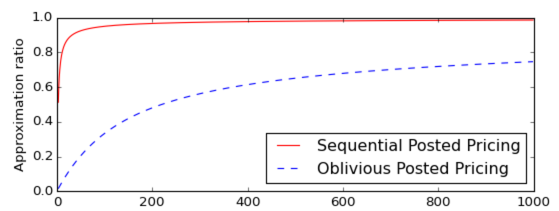
Figure 2: Comparison of the approximation ratios obtained for additive value functions by the two different approaches. On the horizontal axis is $k$, the size of the market.

6 Computing Prices

In the two previous sections, we gave conditions under which optimal prices from the multilinear extension program (5) perform well when offered sequentially or obliviously. In this section, we consider the computational problem of finding these prices. For submodular value functions, we reduce the problem to the well-known greedy algorithm for submodular optimization. For additive value functions, we use a simple method based on the Lagrangian relaxation of the budget constraint.

6.1 The Lagrangian Relaxation for Additive Value Functions

Consider the case of additive value functions where the principal has a value $v_{i}$ for each agent $i$ and the value function is $v(S)=\sum_{i\in S}v_{i}$. Recall the virtual surplus program (2) from Section 3:

$$\max_{\boldsymbol{x}}\ \text{\bf E}_{\boldsymbol{c}}\!\left[v(\boldsymbol{x}(\boldsymbol{c}))\right]$$ (2)

s.t. $$\sum\nolimits_{i}\text{\bf E}_{\boldsymbol{c}}\!\left[\phi_{i}(\boldsymbol{c})\,x_{i}(\boldsymbol{c})\right]\leq B,$$

which can be rewritten for additive value functions as:

$$\max_{\boldsymbol{q}}\ \sum\nolimits_{i}\text{\bf E}_{\boldsymbol{c}}\!\left[v_{i}\,x_{i}(\boldsymbol{c})\right]$$ (6)

s.t. $$\sum\nolimits_{i}\text{\bf E}_{\boldsymbol{c}}\!\left[\phi_{i}(\boldsymbol{c})\,x_{i}(\boldsymbol{c})\right]\leq B.$$

We show that the ex ante optimal mechanism can be found directly by taking the Lagrangian relaxation of the budget constraint (with parameter $\lambda$) of the following Lagrangian program:

$$\max_{\boldsymbol{x}}\ \lambda B+\sum\nolimits_{i}\text{\bf E}_{\boldsymbol{c}}\!\left[(v_{i}-\lambda\phi_{i}(c_{i}))\,x_{i}(\boldsymbol{c})\right].$$ (7)

For any Lagrangian parameter $\lambda$, this objective can be optimized by pointwise optimizing $\sum_{i}(v_{i}-\lambda\phi_{i}(c_{i}))\,x_{i}(\boldsymbol{c})$, a.k.a., the Lagrangian virtual surplus. This pointwise optimization picks all the agents such that $v_{i}\geq\lambda\phi_{i}(c_{i})$. If the virtual cost functions are monotone, i.e., in the so-called regular case, then this optimization gives a monotone allocation rule where an agent is picked whenever $c_{i}\leq\phi_{i}^{-1}(v_{i}/\lambda)$

Notice that as the Lagrangian parameter increases, the payments of the agents, as represented by virtual costs, become more costly in the objective of the lagrangian program (7). Thus, the expected payment of the mechanism is monotonically decreasing in the Lagrangian parameter. With $\lambda=0$ the Lagrangian virtual surplus optimizer simply maximizes $v(\boldsymbol{x})$ and pays each agent selected the maximum cost in the support of her distribution. If this payment is under budget then it is optimal, otherwise, we can increase $\lambda$ until the budget constraint is satisfied. For example, with $\lambda=\infty$ the empty set of agents is selected and no payments are made. The optimal mechanism is the one that meets the budget constraint with equality. In the case that the expected payment is discontinuous then mixing between the least over-budget and least under-budget mechanism is optimal. For further discussion of Lagrangian virtual surplus optimizers, see Devanur et al., (2013).

Proposition .

The Lagrangian virtual surplus optimizer (or appropriate mixture thereof) that meets the budget constraint with equality is the Bayesian optimal ex ante budget feasible mechanism.

Lagrangian virtual surplus optimization suggests selecting an agent $i$ when her private cost $c_{i}$ is below $\phi_{i}^{-1}(v_{i}/\lambda)$. The mechanism that achieves this outcome posts the price of $\hat{c}_{i}=\phi_{i}^{-1}(v_{i}/\lambda)$ to agent $i$. Denote by $\hat{q}_{i}=F_{i}(\hat{c}_{i})$ the probability that $i$ accepts the price $\hat{c}_{i}$. For the prices $\hat{\boldsymbol{c}}$, the total expected payments are $\sum_{i}\hat{c}_{i}\,\hat{q}_{i}$. When the virtual cost functions are monotone and strictly increasing, there is a Lagrangian parameter for which the budget constraint is met with equality, i.e., with $\sum_{i}\hat{c}_{i}\,\hat{q}_{i}=B$. The optimal ex ante mechanism is therefore the posted price mechanism that posts $\hat{c}_{i}$ to each agent $i$ for the Lagrangian parameter $\lambda$ that satisfies $\sum_{i}\hat{c}_{i}\,\hat{q}_{i}=B$. Note that such a Lagrangian parameter $\lambda$ can be arbitrarily well approximated since $\sum_{i}\hat{c}_{i}\,\hat{q}_{i}$ is decreasing as a function of $\lambda$.

Example 1.

Consider $n$ agents with costs drawn uniformly and i.i.d. from $[0,1]$ and uniform additive value function $v_{i}=1$ for all $i$, i.e., the cardinality function. The virtual cost function is $\phi(c)=c+\frac{F(c)}{f(c)}=2c$. The Lagrangian parameter $\lambda=\frac{1}{2}\sqrt{n/B}$ induces a uniform posted price of $\hat{c}=\sqrt{B/n}$ which is accepted with probability $\hat{q}=\sqrt{B/n}$ for an expected payment of $B/n$. Summing over all $n$ agents, the budget is balanced ex ante.

6.2 A Reduction to the Greedy Algorithm for Submodular Optimization

For general submodular value functions we reduce the optimization of the multilinear extension program (5), restated below, to the problem of optimizing a submodular function subject to a cardinality constraint. This problem of optimizing a submodular function under cardinality, knapsack, or matroid constraints is well studied and the greedy algorithm gives a $1-1/e$ approximation for knapsack and cardinality constraints; see Nemhauser et al., (1978), Khuller et al., (1999), and Sviridenko, (2004).

$$\max_{\boldsymbol{q}}\ V(\boldsymbol{q})$$ (5)

s.t. $$\sum\nolimits_{i}q_{i}F_{i}^{-1}(q_{i})\leq B.$$

Define the cost curve of agent $i$ to be the expected payment to agent $i$, i.e., $q_{i}F_{i}^{-1}(q_{i})$ in our case. The main difference between the multilinear extension program (5) and the knapsack setting considered in the literature is that the cost curves in the knapsack setting are linear in $q_{i}$. Our reduction to the greedy algorithm is the following. We divide each agent $i$, called a big agent, in cost space into $m$ discrete agents $i_{j}$ of equal cost, called the small agents. An agent $i_{j}$ corresponds to the $j$th increase of $q_{i}$, starting from $q_{i}=0$, that has cost $B/m$. We set $1/m$ as a fraction of the total budget $B$ which fixes the number of steps in the algorithm to be $m$. With large $m$, the reduction becomes a finer discretization.

Before formally describing the reduction, we introduce some notation. For each $i$ and $j$, let $\delta_{ij}$ be the $j$th increase in $q_{i}$, starting from $q_{i}=0$, that has cost $B/m$, i.e., $\delta_{ij}$ satisfying $B/m=F_{i}^{-1}(\sum_{k\leq j}\delta_{ik})\cdot(\sum_{k\leq j}\delta_{ik})-F_{i}^{-1}(\sum_{k<j}\delta_{ik})\cdot(\sum_{k<j}\delta_{ik})$. Given a set $S$ of small agents, the continuous solution corresponding to $S$ is $\boldsymbol{q}(S)$ with $q_{i}(S)=\sum_{j:i_{j}\in S}\delta_{ij}$.

The reduction.

1. For each agent $i$, create $m$ small agents $i_{j}$ where $1\leq j\leq m$ so that the reduced instance has $mn$ agents.

2. For each small agent $i_{j}$, its cost is $B/m$.

3. For each small agent $i_{j}$, its marginal contribution $V_{S}(i_{j})$ in value to a set $S$ is the marginal contribution of increasing the fraction of agent $i$ corresponding to $S$ by $\delta_{ij}$, i.e., $V(\boldsymbol{q}^{\prime})-V(\boldsymbol{q}(S))$ where $q_{i}^{\prime}=q_{i}(S)+\delta_{ij}$ and $q_{j}^{\prime}=q_{j}(S)$ for $j\neq i$.

We show that the solution to the reduced problem that we obtained with the greedy algorithm for cardinality constraint corresponds to a solution for the multilinear extension program (5) that is a $1-1/e-o(1)$ approximation, almost matching the performance of the greedy algorithm for knapsack constraint with integral agents and linear cost curves. We start by showing that if a solution is feasible in the reduced problem, then the continuous solution corresponding to it is a feasible solution to the multilinear extension program (5). Then, with access to exact values of the increases $\delta_{ij}$ and of the marginal contributions $V_{S}(i_{j})$, the approximation ratio is $1-1/e-o(1)$. Finally, we show that it is possible to approximate $\delta_{ij}$ and $V_{S}(i_{j})$ with estimates that cause an additional loss of $o(1)$ to the approximation ratio.

From a set of small agents to a continuous solution for the big agents.

Previously, we defined a distribution to be regular if the virtual cost function is monotonically increasing. An alternate definition is that a distribution $F$ is regular if the cost curve $q\cdot F^{-1}(q)$ is convex. This definition is the analogue to the revenue curve being concave for regular distributions when the agents are buyers, and not sellers, from Bulow and Roberts, (1989).

Recall that given a set $S$ of small agents, the continuous solution corresponding to $S$ is $\boldsymbol{q}(S)$ with $q_{i}(S)=\sum_{j:i_{j}\in S}\delta_{ij}$ and that $\delta_{ij}$ is the $j$th increase in $q_{i}$ that has cost $B/m$. Therefore, given a set $S$ of small agents of size at most $m$ such that for any $\delta_{ij}\in S$, $\delta_{ik}\in S$ for all $k<j$, then $\boldsymbol{q}(S)$ has cost at most $B$. The condition that if $\delta_{ij}\in S$, then $\delta_{ik}\in S$ for all $k<j$, is equivalent to the condition that greedy always picks small agents corresponding to lower quantiles before small agents corresponding to higher quantiles, which we show formally.

Lemma .

Given two small agents $i_{k}$ and $i_{j}$ such that $k<j$, the greedy algorithm with a cardinality constraint picks $i_{k}$ before $i_{j}$ for regular distributions $F_{i}$.

Proof.

Since all small agents have equal cost, we need to show that $i_{k}$ has a larger marginal contribution than $i_{j}$ to any set $S$ of small agents such that $i_{k},i_{j}\not\in S$. Since $V(\cdot)$ is monotone, it suffices to show that $\delta_{ik}>\delta_{ij}$. In quantile space, the cost of increasing some quantile $q_{i}$ by a fix amount is increasing in $q_{i}$ since $q_{i}\cdot F^{-1}(q_{i})$ is convex by definition of regular distributions. Therefore, in cost space, the increase in quantile $\delta_{i}$ that is obtained by increasing the cost curve by a fix amount is decreasing, so $\delta_{ik}>\delta_{ij}$. ∎

The case of irregular distributions is considered in Section 8.

With exact values of $\delta_{ij}$ and $V_{S}(i_{j})$.

We consider the case where the exact values of the increases in $\boldsymbol{q}$ and marginal contributions are given by an oracle. We show that finding a good solution to this reduced problem with small agents gives us a good solution to the problem with big agents.

Lemma .

The optimal solution $S^{\star}$ to the reduced problem satisfies $V(\boldsymbol{q}(S^{\star}))\geq(1-o(1))V(\hat{\boldsymbol{q}})$ where $\hat{\boldsymbol{q}}$ is the optimal solution to the multilinear extension program (5).

Proof.

We pick the step size to be $m=n^{2}$. The proof shows that there exists a set $S$ that is close to a feasible solution in the reduced problem and such that $\boldsymbol{q}(S)$ is a better solution than $\hat{\boldsymbol{q}}$. Let $S$ be the set of small agents such that $\boldsymbol{q}(S)$ is maximized subject to $\boldsymbol{q}(S)\leq\hat{\boldsymbol{q}}$. Define $S^{+1}$ to be the set containing all small agents in $S$ and one additional small agent for each big agent $i$. Observe that $V(\boldsymbol{q}(S^{+1}))\geq V(\hat{\boldsymbol{q}})$ since $V(\cdot)$ is non-decreasing. So there is a feasible solution to the discretized problem such that if we add one small agent for each big agent $i$, then we obtain a better solution than the optimal solution to the original problem.

Greedily remove agents by minimal marginal contribution from $S^{+1}$ until we get a feasible solution $S$. The number of small agents who need to be removed is $n$ since $S$ is feasible. Since $S$ contains $n^{2}$ small agents, by the greediness and the fact $V(\cdot)$ is concave along any line of positive direction, $(1+1/n)V(\boldsymbol{q}(S))\geq V(\boldsymbol{q}(S^{+1}))$.

Therefore,

$$(1+o(1))V(\boldsymbol{q}(S^{\star}))\geq(1+o(1))V(\boldsymbol{q}(S))\geq V(\boldsymbol{q}(S^{+1}))\geq V(\hat{\boldsymbol{q}})$$

∎

Next, we show that the reduced problem can be optimized.

Lemma .

Let $S$ be the set returned by the greedy algorithm for submodular functions under a cardinality constraint on the reduced problem, then $V(\boldsymbol{q}(S))\geq(1-1/e)V(\boldsymbol{q}(S^{*}))$ where $S^{*}$ is the optimal solution to the reduced problem.

Proof.

Observe that the objective function in the reduced problem is a submodular function. This follows directly from the concavity of $V(\cdot)$ along any positive line of direction. In addition, since all small agents have cost $B/m$, the constraint is a cardinality constraint. Since the greedy algorithm for submodular functions under a cardinality constraint is a $1-1/e$ approximation for submodular functions, we get the desired result. ∎

We now have the tools to show that if we had an oracle for the increases and marginal contributions, the greedy algorithm on the reduced instance would give us a $1-1/e-o(1)$ approximation.

Lemma .

Let $S$ be the output of the greedy algorithm on the reduced instance, where exact values of $\delta_{ij}$ and $V_{S}(i_{j})$ are given by an oracle at each iteration, then $V(\boldsymbol{q}(S))\geq(1-1/e-o(1))V(\hat{\boldsymbol{q}})$, where $\hat{\boldsymbol{q}}$ is the optimal solution to the multilinear extension program (5).

Proof.

We combine the results from the discretization that causes a $o(1)$ loss with the greediness of the algorithm that is a $1-1/e$ approximation to obtain the desired result.

By Lemma 6.2 and Lemma 6.2,

$$V(\boldsymbol{q}(S))\geq(1-1/e)V(\boldsymbol{q}(S^{*}))\geq(1-1/e-o(1))V(\hat{\boldsymbol{q}})$$

where $S^{*}$ is the optimal solution to the reduced problem. ∎

With estimates of $\delta_{ij}$ and $V_{S}(i_{j})$.

We now show that we can use the greedy algorithm with estimates of the increases and the marginal contributions, that we can compute. Let $\tilde{\boldsymbol{q}}(S)$ be defined similarly to $\boldsymbol{q}(S)$ but with estimates $\tilde{\delta}_{i_{j}}$. The first lemma shows that the value of the optimal solution to the reduced problem has almost the same value as when the increases $\delta_{ij}$ are estimated. The second lemma extends Lemma 6.2 to the case where greedy is run with estimated marginal contributions $\tilde{V}_{S}(i_{j})$ and any $\tilde{\delta}_{i_{j}}$. We defer the proofs of these two lemmas to the appendix.

Lemma .

Let $S^{*}$ be the optimal solution to the reduced problem with exact value of $\delta_{ij}$ and $V_{S}(i_{j})$, then $V(\tilde{\boldsymbol{q}}(S^{*}))\geq(1-o(1))V(\boldsymbol{q}(S^{*}))$.

Lemma .

Let $\tilde{S}$ be the set returned by the greedy algorithm on the reduced problem with estimates $\tilde{\delta}_{i_{j}}$ and $\tilde{V}_{S}(i_{j})$, then $V(\tilde{\boldsymbol{q}}(\tilde{S}))\geq(1-1/e-o(1))V(\tilde{\boldsymbol{q}}(S^{*}))$ w.h.p., where $S^{*}$ is the optimal solution to the reduced problem with estimates $\tilde{\delta}_{i_{j}}$ and exact values $V_{S}(i_{j})$.

Combining the previous results, we obtain the main result of this section.

Theorem 9.

Let $\tilde{S}$ be the output by the greedy algorithm on the reduced instance with estimates of $\delta_{ij}$ and $V_{S}(i_{j})$, then $V(\tilde{\boldsymbol{q}}(\tilde{S}))\geq(1-1/e-o(1))V(\hat{\boldsymbol{q}})$ w.h.p., where $\hat{\boldsymbol{q}}$ is the optimal solution to the multilinear extension program (5).

Proof.

This proof follows similarly to the one for Lemma 6.2, the difference is that this proof adds the loss from the estimates.

By Lemma 6.2 and Lemma 6.2,

$$V(\tilde{\boldsymbol{q}}(\tilde{S}))\geq(1-1/e-o(1))V(\tilde{\boldsymbol{q}}(S^{*}))\geq(1-1/e-o(1))V(\boldsymbol{q}(S^{*}))$$

where $S^{*}$ is the optimal solution to the reduced problem. Using Lemma 6.2 that connects the discretized reduced instance to the original continuous problem, we conclude that

$$V(\tilde{\boldsymbol{q}}(\tilde{S}))\geq(1-1/e-o(1))V(\boldsymbol{q}(S^{*}))\geq(1-1/e-o(1))V(\hat{\boldsymbol{q}}).$$

∎

Note that in the case of additive value functions, the greedy algorithm is optimal when the optimization is subject to a cardinality constraint and the marginal contributions can be computed exactly. We therefore get the following result.

Lemma .

Assume $v(\cdot)$ is an additive value function. Let $S$ be the set returned by the greedy algorithm on the reduced problem with estimates $\tilde{\delta}_{i_{j}}$, then $V(\tilde{\boldsymbol{q}}(S))\geq(1-o(1))V(\hat{\boldsymbol{q}})$ w.h.p., where $\hat{\boldsymbol{q}}$ is the optimal solution to the multilinear extension program (5).

Therefore, all the results in previous sections suffer an extra $1-1/e-o(1)$ factor in the general case of submodular value function and an extra $1-o(1)$ factor in the case of additive value function that are due to computational constraints.

7 Symmetric Costs and Values

In this section we study symmetric environments where both the distribution of costs and the value function are symmetric. A submodular value function is symmetric if the value of a set only depends on the cardinality of that set, i.e., $v(S)=g(|S|)$ for some function $g(\cdot)$. In this setting, we obtain an oblivious posted pricing that achieves an approximation ratio of $(1-1/\sqrt{2\pi k})(1-1/k)$ where $k$ is the size of the market, which is identical to the approximation obtained in the additive case with sequential posted pricing. We assume that the distribution of costs is regular.

The following technicalities are used for this section only. We overload the notation and denote by $v(\cdot):\mathbb{R}_{+}\rightarrow\mathbb{R}_{+}$ the concave hull of the points $\{(i,v(S_{i}))\}_{i=0}^{n}$ where $S_{i}$ is any set of size $i$. The posted prices in this section are symmetric and are defined by a single price $\hat{c}$, i.e., $\hat{\boldsymbol{c}}=(\hat{c},\cdots,\hat{c})$ and $\hat{\boldsymbol{q}}=(\hat{q},\cdots,\hat{q})$. Note that the market size $k$ in such a symmetric setting is $k=B/\hat{c}$.

We start with two lemmas that highlight symmetric properties of the optimal solution to the concave closure program in this symmetric setting.

Lemma .

For symmetric submodular value function $v(\cdot)$ and symmetric distributions of costs, the optimal solution $\hat{\boldsymbol{q}}$ to the concave closure program (4) is symmetric, i.e., $\hat{q}_{i}^{+}=\hat{q}_{j}^{+}$ for all $i,j$.

Proof.

By the concavity of the concave closure and the convexity of cost curves (since the distribution of costs is regular), the program we wish to optimize is symmetric and convex, so the optimal solution is symmetric. ∎

Lemma .

For symmetric monotone submodular value function $v(\cdot)$ and symmetric distributions of costs, there exists a distribution ${\cal D}$ over sets of agents with marginals $\hat{\boldsymbol{q}}^{+}=(\hat{q}^{+},\cdots,\hat{q}^{+})$ such that $\text{\bf E}_{S\sim{\cal D}}\!\left[v(S)\right]=V^{+}(\hat{\boldsymbol{q}}^{+})$ and such that all sets $S$ and $T$ that can be drawn from ${\cal D}$ have size either $\lfloor k\rfloor$ or $\lceil k\rceil$.

Proof.

First, note that $B=\hat{c}\cdot n\cdot\hat{q}^{+}$ since $\hat{\boldsymbol{q}}^{+}$ is the optimal solution to the concave closure program and since $v(\cdot)$ is monotone, which implies that $k=n\cdot\hat{q}^{+}$ since $k=B/\hat{c}$.

The expected value of a set of expected size $n\cdot\hat{q}^{+}$ drawn from a distribution is at most $v(n\cdot\hat{q}^{+})$ by the definition of concave hull. By taking a distribution ${\cal D}$ that is a mixture of sets of size $\lfloor n\cdot\hat{q}^{+}\rfloor=\lfloor k\rfloor$ and $\lceil n\cdot\hat{q}^{+}\rceil=\lceil k\rceil$ such that the marginals are $\hat{q}^{+}$, the expected value of a set drawn from ${\cal D}$ is $v(n\cdot\hat{q}^{+})$ since $v(S)$ is submodular. Combining the two previous observations, $\text{\bf E}_{S\sim{\cal D}}\!\left[v(S)\right]=V^{+}(\hat{\boldsymbol{q}}^{+})$ since the concave closure is the maximum expected value over distributions with some marginals $\hat{\boldsymbol{q}}$. ∎

Given quantiles $\hat{\boldsymbol{q}}=(\hat{q},\cdots,\hat{q})$, the value of the concave closure $V^{+}(\hat{\boldsymbol{q}})$ can be computed easily by Lemma 7 and symmetricity. The concave closure program can therefore be approximated arbitrarily well and efficiently when there is symmetry, by using binary search to get arbitrarily close to the optimal quantile $\hat{q}$. Our approach for obtaining the desired approximation is to construct an additive function that lower bounds the symmetric submodular function on feasible sets and that upper bounds it otherwise.

Theorem 10.

In the case of symmetric monotone submodular value functions and symmetric regular cost distributions, the oblivious posted pricing $\hat{\boldsymbol{c}}=(\hat{c},\cdots,\hat{c})$ with $\hat{c}=F^{-1}(\hat{q}^{+})$ is an $(1-1/\sqrt{2\pi k})(1-1/k)$ approximation to the optimal ex ante mechanism, where $\hat{\boldsymbol{q}}^{+}=(\hat{q}^{+},\cdots,\hat{q}^{+})$ is the optimal solution to the concave closure program (4) and $k$ is the size of the market.

Proof.

By Lemma 7, there exists a distribution ${\cal D}$ over sets of agents with marginals $\hat{q}^{+}$ such that $\text{\bf E}_{S\sim{\cal D}}\!\left[v(S)\right]=V^{+}(\hat{\boldsymbol{q}}^{+})$ and such that sets drawn from ${\cal D}$ have size $\lfloor k\rfloor$ or $\lceil k\rceil$. We consider the additive value function $v^{add}(\cdot)$ defined as follow:

$$v^{add}(S)=|S|\frac{v(\lfloor k\rfloor)}{\lfloor k\rfloor}$$

and overload the notation for $v^{add}(\cdot)$ similarly as for $v(\cdot)$. We make the following observations about $v^{add}(\cdot)$:

• $v^{add}(i)\leq v(i)$ for $i\leq\lfloor k\rfloor$ and $v^{add}(i)\geq v(i)$ otherwise, by submodularity.

• $\text{\bf E}_{S\sim{\cal D}}\!\left[v^{add}(S)\right]\geq\text{\bf E}_{S\sim{\cal D}}\!\left[v(S)\right]$, since $v^{add}(\lceil k\rceil)\geq v(\lceil k\rceil)$ and $v^{add}(\lfloor k\rfloor)=v(\lfloor k\rfloor)$.

• $v(\cdot)$ is an additive set function with values $v_{i}=\frac{1}{\lfloor k\rfloor}v(\lfloor k\rfloor)$ for each element.

Since the feasible sets are sets of size at most $\lfloor k\rfloor$ and by the first observation on $v^{add}(\cdot)$, the performance of the posted pricing mechanism is at least the independent integral knapsack value of $v^{add}(\cdot)$. The independent integral knapsack value of $v^{add}(\cdot)$ is at most a factor $(1-1/k)$ away from its independent fractional knapsack value, $\text{\bf E}_{S\sim\hat{\boldsymbol{q}}^{+}}\!\left[v^{add}_{B}(S)\right]$. By Lemma 5 and the third observation on $v^{add}(\cdot)$, $\text{\bf E}_{S\sim\hat{\boldsymbol{q}}^{+}}\!\left[v^{add}_{B}(S)\right]\geq(1-\frac{1}{\sqrt{2\pi k}})\text{\bf E}_{S\sim{\cal D}}\!\left[v^{add}(S)\right]$. By the second observation on $v^{add}(\cdot)$, $\text{\bf E}_{S\sim{\cal D}}\!\left[v^{add}(S)\right]\geq V^{+}(\hat{\boldsymbol{q}}^{+})$. Since $V^{+}(\hat{\boldsymbol{q}}^{+})$ is an upper bound on the optimal mechanism by Lemma 3, we get the desired result. ∎

Note that in previous settings, we used the solution to the multilinear extension program to define the posted pricing mechanisms. In this setting, we used the solution to the concave closure program in order to take advantage of the concavity of the objective function for computational purposes. Finally, note that in the symmetric case, sequential posted pricing offers no advantage compared to oblivious posted pricing.

8 Irregular Distributions

In this section, we consider irregular distributions. Recall that a distribution $F$ is regular if the virtual cost function is increasing, or equivalently, if the cost curve $q\cdot F^{-1}(q)$ is convex. The ironing method introduced by Myerson, (1981) gives monotone ironed virtual costs and convex cost curves. With these convex cost curves, we construct randomized posted pricing mechanisms that enjoy the same approximation ratios as the deterministic mechanisms, albeit with a generalized definition of the market size $k$ for randomized posted pricings. Additionally, in the case of additive objective functions, the sequential posted pricing is derandomized.

Denote the cost curve of agent $i$ by $C_{i}(q_{i})=q_{i}F_{i}^{-1}(q_{i})$. Bulow and Roberts, (1989) observed that the derivative of the cost curve with respect to quantile is equal to the virtual cost function, $C_{i}^{\prime}(q_{i})=\phi_{i}(c_{i})$. The ironing method constructs the convex hull $\bar{C}_{i}(q_{i})$ of the cost curve $C_{i}(\cdot)$. For $q_{i}=F_{i}(c_{i})$, the ironed virtual costs are $\bar{\phi}_{i}(c_{i})=\bar{C}_{i}^{\prime}(q_{i})$. By taking the convex hull of the cost curves, we have convex cost curves and monotone ironed virtual costs as desired. The next two lemmas show that expected payments $\bar{C}_{i}(\hat{q}_{i})$ are feasible while serving each agent with probability $\hat{q}_{i}$, and that no incentive compatible mechanism can do better.

Lemma (Myerson,, 1981, Bulow and Roberts,, 1989).

For any agent with cost drawn from distribution $F_{i}$ and any incentive compatible mechanism that selects agent $i$ with probability $\hat{q}_{i}$, the expected payment to agent $i$ is at least $\bar{C}_{i}(\hat{q}_{i})$.

We give the proof of the following known lemma since it exhibits how to pick the prices and the probabilities of the randomized mechanisms.

Lemma (Myerson,, 1981).

Expected payment $\bar{C}_{i}(\hat{q}_{i})$ while serving agent $i$ with probability $\hat{q}_{i}$ is achievable using a randomized posted pricing with at most two prices.

Proof.

Fix a seller $i$ and an ex ante sale probability $\hat{q}_{i}$. If $\hat{q}_{i}=C_{i}(\hat{q}_{i})$, then it suffices to post price $F_{i}^{-1}(\hat{q}_{i})$. Otherwise, let $a$ be the largest quantile smaller than $\hat{q}_{i}$ such that $\bar{C}_{i}(a)=C_{i}(a)$. Similarly, let $b$ the smallest quantile larger than $\hat{q}_{i}$ such that $\bar{C}_{i}(b)=C_{i}(b)$. The interval $[a,b]$ corresponds to the ironed interval in which $\hat{q}_{i}$ falls in. By the definition of convex hull, we get

$$\bar{C}_{i}(\hat{q}_{i})=(1-\frac{\hat{q}_{i}-a}{b-a})\bar{C}_{i}(a)+(1-\frac{b-\hat{q}_{i}}{b-a})\bar{C}_{i}(b)=(1-\frac{\hat{q}_{i}-a}{b-a})C_{i}(a)+(1-\frac{b-\hat{q}_{i}}{b-a})C_{i}(b).$$

Therefore, posting price $F_{i}^{-1}(a)$ with probability $1-\frac{\hat{q}_{i}-a}{b-a}$ and $F_{i}^{-1}(b)$ with probability $1-\frac{b-\hat{q}_{i}}{b-a}$ has expected payment $\bar{C}_{i}(\hat{q}_{i})$ and the ex ante probability that seller $i$ accepts the price is $\hat{q}_{i}$. ∎

By Lemma 8 and Lemma 8, the ex ante results also hold for the irregular case using randomized posted pricing. The following definition generalizes the notion of posted prices to allow for randomization.

Definition 6.

For a randomized posted pricing $\hat{\boldsymbol{q}}$,

• Prices $\hat{c}_{i1}$ and $\hat{c}_{i2}$ with probabilities of picking each price are induced by $\hat{q}_{i}$.

• Randomly pick $\hat{c}_{i1}$ or $\hat{c}_{i2}$.

• In the case of sequential posted pricing, set the ordering to be in decreasing order of bang-per-buck.

Definition 7.

With randomized posted pricing, a market is $k$-large if $B/\hat{c}_{ij}\geq k$ for all agents $i$ and $j\in\{1,2\}$.

8.1 From Ex Ante to Ex Post with Additive Value Functions

For the additive case, we first show that the ex post randomized posted pricing performs well and then derandomize the mechanism.

Theorem 11.

The randomized sequential posted pricing mechanism $(\hat{\boldsymbol{q}},\boldsymbol{\sigma}(\cdot))$ that serve agents with probability $\hat{\boldsymbol{q}}$, where $\hat{\boldsymbol{q}}$ is the solution to the multilinear extension program (5) and where the order $\boldsymbol{\sigma}(\cdot)$ is decreasing in $\frac{v_{i}}{\hat{c}_{i}}$, is a $(1-1/\sqrt{2\pi k})(1-1/k)$ approximation to the optimal mechanism in a $k$-large market.

Proof.

We show that the randomized sequential posted pricing performs better than a deterministic sequential posted pricing with the same ex ante performance and a market that is $k$-large. Consider a randomized agent $i$ who is offered $\hat{c}_{i}=\hat{c}_{i1}$ with probability $\rho$ and $\hat{c}_{i}=\hat{c}_{i2}$ otherwise. Remove agent $i$ and replace it with two deterministic agents $i1$ and $i2$ with value $v_{i}$, who are offered $\hat{c}_{i1}$ and $\hat{c}_{i2}$ and who accept their price with probability $\rho F_{i}(\hat{c}_{i1})$ and $(1-\rho)F_{i}(\hat{c}_{i2})$ respectively. Call this new posted pricing the deterministic instance and the original posted pricing the randomized instance.

Both instances have the same ex ante performance since the expected total cost remains the same and since agent $i$ accepts his offer with probability equal to the sum of the probabilities that agents $i_{1}$ and $i_{2}$ accept their offer. Fix a set $S$ of agents who accept their offer that does not include $i$ and fix these offers. Notice that in both the randomized and deterministic instance, there is an expected increase in the total cost of $\hat{c}_{i1}\rho F_{i}(\hat{c}_{i1})+\hat{c}_{i2}(1-\rho)F_{i}(\hat{c}_{i2})$ caused by agent $i$ to $S$. However, in the randomized instance, this increase in cost is either $\hat{c}_{i1}$ or $\hat{c}_{i2}$ and in the deterministic instance, this increase in cost can also be $\hat{c}_{i1}+\hat{c}_{i2}$. Since agents are ordered by decreasing bang-per-buck, the loss from agents that do not fit in the ex post budget constraint is greater in the deterministic case. Therefore, the loss of the fractional knapsack value with respect to the ex ante performance of the mechanism is greater in the deterministic instance.

Now note that this argument can be repeated inductively until all the agents left are deterministic. So the approximation ratio obtained by the randomized mechanism is $(1-1/\sqrt{2\pi k})(1-1/k)$, by combining Lemma 5 and the $1-1/k$ loss from dropping the fractional agent. ∎

We now show that the mechanism can be derandomized.

Theorem 12.

Any sequential randomized posted pricing $(\hat{\boldsymbol{q}},\boldsymbol{\sigma}(\cdot))$ can be modified into a sequential deterministic posted pricing in the case of additive value functions.

Proof.

The proof proceeds in two steps. The first reduces the number of randomized agents until there is one left by using properties of ironed intervals. The second step is to simply pick the best of the two prices that are offered to the last randomized agent.

Consider a randomized posted pricing $(\hat{\boldsymbol{q}},\boldsymbol{\sigma}(\cdot))$ with at least two agents $i$ and $j$ that are randomized. The marginal cost per unit value of these two agents are $\bar{C}_{i}^{\prime}(\hat{q}_{i})/v_{i}=\bar{\phi}_{i}(c_{i})/v_{i}$ and $\bar{\phi}_{j}(c_{j})/v_{j}$. Without loss of generality, assume $\bar{\phi}_{i}(c_{i})/v_{i}\leq\bar{\phi}_{j}(c_{j})/v_{j}$. Since both of these agents are randomized, $\hat{q}_{i}$ and $\hat{q}_{j}$ are within ironed intervals and their ironed virtual costs are constants within these intervals. With no loss in the objective function, we can therefore increase $\hat{q}_{i}$ and decrease $\hat{q}_{j}$ such that the budget still binds and such that either $\hat{q}_{i}$ or $\hat{q}_{j}$ is at the extremity of the ironed interval it is in, and therefore not randomized anymore. This construction can be repeated until one randomized agent is left.

Consider a randomized posted pricing with a unique randomized agent $i$ who is offered $\hat{c}_{i}=\hat{c}_{i1}$ with probability $\rho$ and $\hat{c}_{i}=\hat{c}_{i2}$ otherwise. The proof of Theorem 11 shows that the ratio between the performance of the optimal mechanism and the expected fractional knapsack value is at least $1-1/\sqrt{2\pi k}$. Agent $i$ is either offered $\hat{c}_{i1}$ or $\hat{c}_{i2}$, so by expectations, with at least one of these two offers, the previous ratio is at least $1-1/\sqrt{2\pi k}$. Dropping the fractional agent and keeping the best price to offer to agent $i$, we therefore get a $(1-1/\sqrt{2\pi k})(1-1/k)$ approximation for a deterministic mechanism. ∎

Corollary .

Any sequential randomized posted pricing $(\hat{\boldsymbol{q}},\boldsymbol{\sigma}(\cdot))$ can be modified with high probability into a sequential deterministic posted pricing in the case of additive value functions with an additional $o(1)$ loss in polynomial time.

Proof.

We need to compute which offered price between $\hat{c}_{i1}$ and $\hat{c}_{i2}$ performs better in terms of fractional knapsack value. Fractional-knapsack is a submodular function and the multilinear extension of submodular functions can be approximated arbitrarily well by sampling using Chernoff bounds. Therefore, with high probability, it is possible to compare arbitrarily well the fractional knapsack value obtained with the two offered prices to agent $i$. ∎

8.2 From Ex Ante to Ex Post with Submodular Value Functions

With submodular value functions, the analysis for the oblivious randomized posted pricing is identical as the analysis for the oblivious deterministic posted pricing. In Section 4, Theorem 5 shows that by lowering the budget by some small amount, we get that the sum of the costs does not exceed the budget with high probability. Note that this results does not only hold for deterministic agents but also for randomized agents since the payment $p_{i}$ to an agent $i$ only need to be bounded by $B/k$ and is not restricted to be either $0$ or $\hat{c}_{i}$. Therefore, the sum of the costs does not exceed the budget with high probability in the randomized case as well and the remaining of the analysis of section 4 also holds.

Theorem 13.

For $\epsilon\in(0,1/2)$, if the randomized oblivious posted pricing $\hat{\boldsymbol{q}}$, where $\hat{\boldsymbol{q}}$ is the optimal solution to the multilinear extension program (5) with budget $(1-\epsilon)B$, satisfies $2/\epsilon\leq k\leq B/\max_{i}\hat{c}_{i}$, then this posted pricing mechanism is a $(1-1/e)(1-\epsilon)(1-e^{-\epsilon^{2}(1-\epsilon)k/12})$ approximation to the optimal mechanism for submodular value functions and $(1-\epsilon)(1-e^{-\epsilon^{2}(1-\epsilon)k/12})$ for additive value functions.

9 Conclusion

We consider questions of budget feasibility in a Bayesian setting. We show that simple posted pricing mechanisms are ex post budget feasible and approximate the Bayesian optimal mechanism. Our analysis first considers the ex ante relaxation where the budget constraint is allowed to hold in expectation. Good approximations are obtained when this ex ante relaxation is optimized for a slightly reduced budget or when the agents are ordered by bang-per-buck (value divided by offered price). The latter approach, in the case of additive value functions when it applies, gives better bounds.

Another method for designing posted pricing mechanisms from the literature comes from the generalized magician’s problem from Alaei, (2014). Unfortunately, this approach does not satisfy the monotonicity property of Theorem 4 needed to apply known results that give a good approximation in the case of submodular functions. Thus, it is unclear whether this approach can be adapted to budget feasibility questions.

APPENDIX

Missing proofs from section 6

Proof of Lemma 6.2.

We need to find the increase satisfies $B/m=F_{i}^{-1}(\sum_{k\leq j}\delta_{i_{k}})\cdot(\sum_{k\leq j}\delta_{i_{k}})-F_{i}^{-1}(\sum_{k<j}\delta_{i_{k}})\cdot(\sum_{k<j}\delta_{i_{k}})$. To approximate it, we find $\tilde{\delta}_{i_{j}}$ such that $(1-1/n^{3})\delta_{i_{j}}\leq\tilde{\delta}_{i_{j}}\leq\delta_{i}$, which can be done easily since the weight functions are increasing.

Recall that $\tilde{\boldsymbol{q}}(S)$ is defined similarly to $\boldsymbol{q}(S)$ but with estimates $\tilde{\delta}_{i_{j}}$. Let $S^{\star}$ be the optimal solution of the problem with small agents without noise. Since $(1-1/n^{3})\delta_{i_{j}}\leq\tilde{\delta}_{i_{j}}\leq\delta_{i_{j}}$ for all $i,j$, we get that $\tilde{\boldsymbol{q}}(S^{\star})\geq(1-1/n)\boldsymbol{q}(S^{\star})$. By the concavity of $V(\cdot)$ along positive lines of direction, we get that $V(\tilde{\boldsymbol{q}}(S^{\star}))\geq(1-1/n)V(\boldsymbol{q}(S^{\star}))$. ∎

Proof of Lemma 6.2.

First note that the objective function for the reduced instance is a submodular function regardless of the values of $\tilde{\delta}_{i_{j}}$. So since we are comparing ourselves with $\tilde{\boldsymbol{q}}(S^{*})$, it remains to show that the greedy algorithm with a noisy oracle on marginal contribution of agents performs well.

Let $g(\cdot)$ be the objective function of the reduced instance. The marginal contributions are estimated by taking $\frac{10}{\delta^{4}}(1+\ln n)$ samples of the random set with independent marginal probabilities $\boldsymbol{q}$. By using basic Chernoff bounds as in Calinescu et al., (2011), we get that with high probability, all the estimates that are computed during the algorithm have an additive error of at most $\delta^{2}g(S^{\star})$.

Let $S$ be the set of small agents returned by the algorithm. Let $S_{i}=\{e_{1},\dots,e_{i}\}$ be the value of $S$ after $i$ iterations. Now since $g(\cdot)$ is submodular,

$$g(S^{\star}) \leq g(S_{i-1})+\sum_{e\in S^{\star}\setminus S_{i-1}}g_{S_{i-1}}(e)$$

By the greediness of the algorithm, $\tilde{g}_{S_{i-1}}(e_{i})\geq\tilde{g}_{S_{i-1}}(e)$ for all $e\in S^{\star}\setminus S_{i-1}$. So, $g_{S_{i-1}}(e_{i})+2\delta^{2}g(S^{\star})\geq g_{S_{i-1}}(e)$, and

$$g(S^{\star}) \leq g(S_{i-1})+\frac{1}{\delta}(g_{S_{i-1}}(e_{i})+2\delta^{2}g(S^{\star}))$$

$$(1-2\delta)g(S^{\star}) \leq g(S_{i-1})+\frac{1}{\delta}g_{S_{i-1}}(e_{i})$$

Then, by following identically the remaining of the proof for the $e/(e-1)$ approximation for greedy subject to a cardinality constraint, but by replacing $g(S^{\star})$ by $(1-2\delta)g(S^{\star})$, we get that $(1-1/e)g(S)\geq(1-2\delta)g(S^{\star})$, which concludes the proof. ∎

References

- Agrawal et al., (2010) Agrawal, S., Ding, Y., Saberi, A., and Ye, Y. (2010). Correlation robust stochastic optimization. In Proceedings of the twenty-first annual ACM-SIAM symposium on Discrete Algorithms, pages 1087–1096. Society for Industrial and Applied Mathematics.
- Alaei, (2014) Alaei, S. (2014). Bayesian combinatorial auctions: Expanding single buyer mechanisms to many buyers. SIAM Journal on Computing, 43(2):930–972.
- Anari et al., (2014) Anari, N., Goel, G., and Nikzad, A. (2014). Mechanism design for crowdsourcing: An optimal 1-1/e competitive budget-feasible mechanism for large markets. In Foundations of Computer Science (FOCS), 2014 IEEE 55th Annual Symposium on, pages 266–275. IEEE.
- Badanidiyuru et al., (2012) Badanidiyuru, A., Kleinberg, R., and Singer, Y. (2012). Learning on a budget: posted price mechanisms for online procurement. In Proceedings of the 13th ACM Conference on Electronic Commerce, pages 128–145. ACM.
- Bansal et al., (2010) Bansal, N., Korula, N., Nagarajan, V., and Srinivasan, A. (2010). On k-column sparse packing programs. In Integer Programming and Combinatorial Optimization, pages 369–382. Springer.
- Bei et al., (2012) Bei, X., Chen, N., Gravin, N., and Lu, P. (2012). Budget feasible mechanism design: from prior-free to bayesian. In Proceedings of the forty-fourth annual ACM symposium on Theory of computing, pages 449–458. ACM.
- Bulow and Roberts, (1989) Bulow, J. and Roberts, J. (1989). The simple economics of optimal auctions. The Journal of Political Economy, pages 1060–1090.
- Calinescu et al., (2007) Calinescu, G., Chekuri, C., Pál, M., and Vondrák, J. (2007). Maximizing a submodular set function subject to a matroid constraint. In Integer programming and combinatorial optimization, pages 182–196. Springer.
- Calinescu et al., (2011) Calinescu, G., Chekuri, C., Pál, M., and Vondrák, J. (2011). Maximizing a monotone submodular function subject to a matroid constraint. SIAM Journal on Computing, 40(6):1740–1766.
- Chawla et al., (2010) Chawla, S., Hartline, J. D., Malec, D. L., and Sivan, B. (2010). Multi-parameter mechanism design and sequential posted pricing. In Proceedings of the forty-second ACM Symposium on Theory of Computing, pages 311–320. ACM.
- Chawla et al., (2012) Chawla, S., Hartline, J. D., and Sivan, B. (2012). Optimal crowdsourcing contests. In Proceedings of the twenty-third annual ACM-SIAM symposium on discrete algorithms, pages 856–868. SIAM.
- Chen et al., (2011) Chen, N., Gravin, N., and Lu, P. (2011). On the approximability of budget feasible mechanisms. In Proceedings of the twenty-second annual ACM-SIAM symposium on Discrete Algorithms, pages 685–699. SIAM.
- Devanur et al., (2013) Devanur, N. R., Ha, B. Q., and Hartline, J. D. (2013). Prior-free auctions for budgeted agents. In Proceedings of the Fourteenth ACM Conference on Electronic Commerce, pages 287–304. ACM.
- Ensthaler and Giebe, (2014) Ensthaler, L. and Giebe, T. (2014). Bayesian optimal knapsack procurement. European Journal of Operational Research, 234(3):774–779.
- Esö and Futo, (1999) Esö, P. and Futo, G. (1999). Auction design with a risk averse seller. Economics Letters, 65(1):71–74.
- Ho et al., (2015) Ho, C.-J., Slivkins, A., Suri, S., and Vaughan, J. W. (2015). Incentivizing high quality crowdwork. In Proceedings of the 24th International Conference on World Wide Web, pages 419–429. International World Wide Web Conferences Steering Committee.
- Immorlica et al., (2015) Immorlica, N., Stoddard, G., and Syrgkanis, V. (2015). Social status and badge design. In Proceedings of the 24th International Conference on World Wide Web, pages 473–483. International World Wide Web Conferences Steering Committee.
- Khuller et al., (1999) Khuller, S., Moss, A., and Naor, J. S. (1999). The budgeted maximum coverage problem. Information Processing Letters, 70(1):39–45.
- Myerson, (1981) Myerson, R. (1981). Optimal auction design. Mathematics of Operations Research, 6:58–73.
- Myerson and Satterthwaite, (1983) Myerson, R. and Satterthwaite, M. (1983). Efficient mechanisms for bilaterial trade. Journal of Economic Theory, 29:265–281.
- Nemhauser et al., (1978) Nemhauser, G. L., Wolsey, L. A., and Fisher, M. L. (1978). An analysis of approximations for maximizing submodular set functions—i. Mathematical Programming, 14(1):265–294.
- Singer, (2010) Singer, Y. (2010). Budget feasible mechanisms. In The 51st Annual IEEE Symposium on Foundations of Computer Science, pages 765–774. IEEE.
- Singer and Mittal, (2013) Singer, Y. and Mittal, M. (2013). Pricing mechanisms for crowdsourcing markets. In Proceedings of the 22nd international conference on World Wide Web, pages 1157–1166. International World Wide Web Conferences Steering Committee.
- Singla and Krause, (2013) Singla, A. and Krause, A. (2013). Truthful incentives in crowdsourcing tasks using regret minimization mechanisms. In Proceedings of the 22nd international conference on World Wide Web, pages 1167–1178. International World Wide Web Conferences Steering Committee.
- Sviridenko, (2004) Sviridenko, M. (2004). A note on maximizing a submodular set function subject to a knapsack constraint. Operations Research Letters, 32(1):41–43.
- Vondrák et al., (2011) Vondrák, J., Chekuri, C., and Zenklusen, R. (2011). Submodular function maximization via the multilinear relaxation and contention resolution schemes. In Proceedings of the forty-third annual ACM symposium on Theory of computing, pages 783–792. ACM.
- Yan, (2011) Yan, Q. (2011). Mechanism design via correlation gap. In Proceedings of the twenty-second annual ACM-SIAM symposium on Discrete Algorithms, pages 710–719. SIAM.