Critical behavior of the Higgs- and Goldstone-mass gaps for the two-dimensional model
Abstract
Spectral properties for the two-dimensional quantum model were investigated with the exact diagonalization method. In the symmetry-broken phase, there appear the massive Higgs and massless Goldstone excitations, which correspond to the longitudinal and transverse modes of the spontaneous magnetic moment, respectively. The former excitation branch is embedded in the continuum of the latter, and little attention has been paid to the details, particularly, in proximity to the critical point. The finite-size-scaling behavior is improved by extending the interaction parameters. An analysis of the critical amplitude ratio for these mass gaps is made.
keywords:
75.10.Jm 75.40.Mg 05.50.+q , 05.70.Jk1 Introduction
In the symmetry-broken phase, the O-symmetric system, such as the model, exhibits a massless Goldstone excitation, which corresponds to the transverse modulation of the magnetic moment. On the one hand, the longitudinal mode, namely, the Higgs excitation, is massive, embedded in the continuum of the former; see Ref. [1] for a review. The O- [equivalently, U-] symmetric system is ubiquitous in nature, and such a characteristic spectrum has been observed for a variety of substances [2, 3, 4, 5, 6, 7, 8, 9, 10, 11]. The perturbation field (experimental probe) should retain the O (axial) symmetry [1, 12, 13, 14, 15]; otherwise, the contribution from the Goldstone excitations smears out the Higgs-mode branch [16, 17, 18, 19]. (For instance, the chemical-potential modulation for the bosonic system does not conflict with the symmetry.)
Recent studies [20, 21] shed light on a universal character of the spectrum in proximity to the phase transition, especially, in dimensions; it would be intriguing that the spectral property is also under the reign of universality. In dimensions, the criticality is described simply by the Ginzburg-Landau theory (Gaussian fixed point). On the contrary, in dimensions, the spectral property is non-perturbative by nature. In particular, a universal amplitude ratio for the mass gaps [see Eq. (1) mentioned afterward] is arousing much attention recently.
In this paper, we investigate the two-dimensional quantum -spin model (2) with the exact diagonalization method. The method enables us to calculate the low-lying level indexed by quantum numbers. In order to suppress corrections to scaling, we incorporate various types of interaction parameters in addition to the ordinary nearest-neighbor ferromagnetic interaction . Thereby, we investigate the universality for the critical amplitude ratio
| (1) |
with the Higgs mass , the Goldstone mass , and the reflected gap with respect to the critical point ; technical details and underlying physics are explained in the next section. The amplitude ratio has been estimated as [22, 23] and [24] by means of the (quantum) Monte Carlo method. According to the recent elaborated renormalization-group analyses, the ratio was estimated as [25], [26], and [27].
To be specific, we present the Hamiltonian for the model [28]
| (2) | |||||
Here, the quantum -spin operator is placed at each square-lattice point . The summations, , , and , run over all possible nearest-neighbor, next-nearest-neighbor, and plaquette spins, respectively. The parameters are the corresponding coupling constants. The parameter denotes the single-ion anisotropy. We survey the coupling-constant subspace
| (3) |
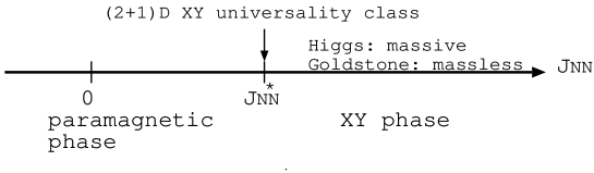
parameterized by . At , the system undergoes a phase transition; a schematic phase diagram is presented in Fig. 1. Here, the critical point
| (4) |
was adjusted [28] to an IR fixed point with almost eliminated irrelevant interactions; that is, the coupling constants were determined through an approximative real-space renormalization group, and the remaining one was finely tuned via the conventional finite-size-scaling analysis. As shown in Eq. (2), the -spin model allows us to incorporate various interactions such as the single-ion anisotropy, with which one is able to realize the -paramagnetic phase transition. In this sense, the extention of the magnetic moment to is essential in our study.
2 Numerical results
In this section, we present the simulation results. To begin with, we explain the simulation technique.
2.1 Simulation algorithm
In this section, we explain the simulation algorithm. As mentioned in Introduction, the model (2) was simulated with the exact diagonalization method. We implemented the screw-boundary condition [29] in order to treat a variety of system sizes (: number of constituent spins) systematically; note that conventionally, the system size is restricted within . We adopt the algorithm presented in Sec. II of Ref. [28]. The linear dimension is given by ; note that the spins constitute a rectangular cluster.
Thereby, we evaluated the mass gaps and via the following scheme. The exact diagonalization method yields the low-lying energy levels explicitly. Each level is specified by the momentum and the perpendicular magnetic moment ; in practice, the numerical diagonalization was performed within the subspace . The Higgs- and Goldstone-mass gaps are characterized by
| (5) |
and
| (6) |
respectively. The reflected gap with respect to the critical point is calculated by . The gap () becomes massive in the paramagnetic () phase (), and hence, the ratio makes sense in the phase. The gap is interpreted as the insulator gap through regarding the ladder operators as the bosonic creation-annihilation operators.
2.2 Scaling analyses of
In Fig. 2, we present the scaled Higgs gap for the nearest-neighbor ferromagnetic interaction and various system sizes (). The data merge around , indicating an onset of criticality; note that the scaled energy gap should be scale-invariant at the critical point. The location of the critical point is consistent with Eq. (4). The Higgs gap appears to open in both the paramagnetic () and ( ) phases; the latter case is our main concern, as mentioned in Introduction.
In Fig. 3, we present the scaled Goldstone gap for various and . The data indicate an onset of criticality around . The Goldstone gap closes in the phase, while it opens in the paramagnetic phase. The latter gap is interpreted as the (bosonic) insulator gap , setting a fundamental energy scale in this domain; actually, the transition is interpreted as the superfluid-insulator transition [21]. Hence, the ratio , Eq. (1), makes sense in the phase, and the criticality is investigated in the next section.
In Fig. 4, we present the scaling plot, -, for various system sizes . Here, the scaling parameters are set to [Eq. (4)] and [30, 31]. The data appear to collapse into a scaling curve satisfactorily. Similarly, in Fig. 5, we present the scaling plot, -, for various system sizes ; the scaling parameters are the same as those of Fig. 4.
We address a few remarks. First, the data in Figs. 4 and 5 collapse into the scaling curves satisfactorily. Such a feature indicates that corrections to scaling are almost negligible owing to the fine adjustment [28] of the coupling constants to Eq. (4). Because the tractable system size with the exact diagonalization method is severely restricted, it is significant to accelerate the convergence to the scaling limit. Second, the scaling parameters, and , are taken from the literatures, Refs. [28] and [30], respectively. That is, there are no adjustable ad hoc parameters in the present scaling analyses. Last, as demonstrated in Figs. 2 and 3, both mass gaps possess an identical scaling dimension. Hence, the amplitude ratio (1) makes sense, and the criticality is explored in the next section.
2.3 Analysis of the amplitude ratio
In this section, encouraged by the findings in Sec. 2.2, we turn to the analysis of the amplitude ratio , Eq. (1).
In Fig. 6, we present the scaling plot, -, for ; here, the scaling parameters, and , are the same as those of Fig. 4. In the phase, , the amplitude ratio exhibits a plateau for an appreciable range of . Such a feature clearly indicates that the amplitude ratio is a universal constant in this domain.
Upon close inspection, the plateaux in Fig. 6 are curved concavely. The shallow bottom locates at , satisfying for each system size . We regard the bottom height
| (7) |
as an indicator for . The amplitude ratio (7) is plotted for [] in Fig. 7. The least-squares fit to the data yields an estimate in the thermodynamic limit . As a reference, a similar analysis was performed with the abscissa scale replaced with , and we arrived at . The discrepancy between these estimates appears to dominate the least-squares-fit error , and the discrepancy may indicate an ambiguity as to the extrapolation (systematic error). Regarding it as a possible systematic error, we estimate the amplitude ratio as
| (8) |
A comment may be in order, the series of data in Fig. 7 appear to be oscillatory; actually, we observe a slight bump around . Such an oscillatory behavior is an artifact of the screw-boundary condition [29], rendering an ambiguity as to the extrapolation to . The ambiguity appears to be bounded by the above-mentioned error margin, which is estimated by performing two independent extrapolation schemes.
3 Summary and discussions
The critical behavior of was investigated for the two-dimensional quantum model (2) by means of the numerical diagonalization method [29, 28]. The interaction parameters were adjusted to Eq. (3) in order to suppress corrections to scaling [28]. As a consequence, the data (Figs. 4 and 5) collapse into the scaling curves satisfactorily, indicating that the data already enter the scaling regime. Thereby, we confirm a universal character for the mass-gap ratio (Fig. 6), and estimate the amplitude ratio as .
As mentioned in Introduction, the amplitude ratio has been estimated with the (quantum) Monte Carlo method, [22, 23] and [24], as well as the renormalization-group approaches, [25], [26], and [27]. According to the Ginzburg-Landau (mean-field) theory, the amplitude ratio should be . Clearly, the spectral property reveals a notable deviation from that anticipated from the mean-field theory; the Ising counterpart was studied in Ref. [32]. In this respect, detailed analyses of other spectral properties such as the AC conductivity [23, 33] would be desirable. A progress toward this direction is left for the future study.
Acknowledgment
This work was supported by a Grant-in-Aid for Scientific Research (C) from Japan Society for the Promotion of Science (Grant No. 25400402).


References
- [1] D. Pekker and C.M. Varma, Annual Rev. Condens. Matter Phys. 6 (2015) 269.
- [2] Ch. Rüegg, B. Normand, M. Matsumoto, A. Furrer, D. F. McMorrow, K. W. Krämer, H. -U. Güdel, S. N. Gvasaliya, H. Mutka, and M. Boehm, Phys. Rev. Lett. 100 (2008) 205701.
- [3] U. Bissbort, S. Götze, Y. Li, J. Heinze, J. S. Krauser, M. Weinberg, C. Becker, K. Sengstock, and W. Hofstetter, Phys. Rev. Lett. 106 (2011) 205303.
- [4] M. Endres, T. Fukuhara, D. Pekker, M. Cheneau, P. Schauß, C. Gross, E. Demler, S. Kuhrand, and I. Bloch, Nature 487 (2012) 454.
- [5] J. Demsar, K. Biljaković, and D. Mihailovic, Phys. Rev. Lett. 83 (1999) 800.
- [6] R. Yusupov, T. Mertelj, V. V. Kabanov, S. Brazovskii, P. Kusar, J.-H. Chu, I. R. Fisher and D. Mihailovic, Nature Phys. 6 (2010) 681.
- [7] K. B. Lyons, P. A. Fleury, J. P. Remeika, A. S. Cooper, and T. J. Negran, Phys. Rev. B 37 (1988) 2353.
- [8] J.B. Parkinson, J. Phys. C Solid State Phys. 2 (1969) 2003.
- [9] P. A. Fleury and H. J. Guggenheim, Phys. Rev. Lett. 24 (1970) 1346.
- [10] R. J. Elliott and M. F. Thorpe, J. Phys. C Solid State Phys. 2 (1969) 1630.
- [11] B. S. Shastry and B. I. Shraiman, Phys. Rev. Lett. 65 (1990) 1068.
- [12] N. H. Lindner and A. Auerbach, Phys. Rev. B 81 (2010) 054512.
- [13] D. Podolsky, A. Auerbach, and D. P. Arovas, Phys. Rev. B 84 (2011) 174522.
- [14] S. D. Huber, E. Altman, H. P. Büchler, and G. Blatter, Phys. Rev. B 75 (2007) 085106.
- [15] S. D. Huber, B. Theiler, E. Altman, and G. Blatter, Phys. Rev. Lett. 100 (2008) 050404.
- [16] A. V. Chubukov, S. Sachdev, and J. Ye, Phys. Rev. B 49 (1994) 11919.
- [17] S. Sachdev, Phys. Rev. B 59 (1999) 14054.
- [18] W. Zwerger, Phys. Rev. Lett. 92 (2004) 027203.
- [19] N. Dupuis, Phys. Rev. A 80 (2009) 043627.
- [20] D. Podolsky and S. Sachdev, Phys. Rev. B 86 (2012) 054508.
- [21] L. Pollet and N. Prokof’ev, Phys. Rev. Lett. 109 (2012) 010401.
- [22] S. Gazit, D. Podolsky, and A. Auerbach, Phys. Rev. Lett. 110 (2013) 140401.
- [23] S. Gazit, D. Podolsky, A. Auerbach, and D. P. Arovas, Phys. Rev. B 88 (2013) 235108.
- [24] K. Chen, L. Liu, Y. Deng, L. Pollet, and N. Prokof’ev, Phys. Rev. Lett. 110 (2013) 170403.
- [25] A. Rançon and N. Dupuis, Phys. Rev. B 89 (2014) 180501.
- [26] F. Rose, F. Léonard and N. Dupuis, Phys. Rev. B 91 (2015) 224501.
- [27] Y. T. Katan and D. Podolsky, Phys. Rev. B 91 (2015) 075132.
- [28] Y. Nishiyama, Phys. Rev. E 78 (2008) 021135.
- [29] M.A. Novotny, J. Appl. Phys. 67 (1990) 5448.
- [30] M. Campostrini, M. Hasenbusch, A. Pelissetto, and E. Vicari, Phys. Rev. B 74 (2006) 144506.
- [31] E. Burovski, J. Machta, N. Prokof’ev, and B. Svistunov, Phys. Rev. B 74 (2006) 132502.
- [32] S. Dusuel, M. Kamfor, K.P. Schmidt, R. Thomale, and J. Vidal, Phys. Rev. B 81 (2010) 064412.
- [33] K. Chen, L. Liu, Y. Deng, L. Pollet, and N. Prokof’ev, Phys. Rev. Lett. 112 (2014) 030402.