Occam’s Gates

Abstract

We present a complimentary objective for training recurrent neural networks (RNN) with gating units that helps with regularization and interpretability of the trained model. Attention-based RNN models have shown success in many difficult sequence to sequence classification problems with long and short term dependencies, however these models are prone to overfitting. In this paper, we describe how to regularize these models through an L1 penalty on the activation of the gating units, and show that this technique reduces overfitting on a variety of tasks while also providing to us a human-interpretable visualization of the inputs used by the network. These tasks include sentiment analysis, paraphrase recognition, and question answering.

1 Introduction

Attention-based recurrent neural networks (RNN) have shown great success in a wide range of tasks such as computer vision [1, 2, 3],image generation [4, 5], machine translation [6], speech recognition [7], or even as controllers for memory addressing and retrieval [8, 9].

While there is debate as to how biologically plausible these cognition models are, they are desirable in their ability to allow introspection into the network’s workings and understanding failures: in the case of image captioning [2, 1] and generation [4, 5], or emotion detection [10], the system’s focus matches up with human intuition. The gates modulating the network’s attention in these networks serve a dual purpose: first they allow control of the information flow, and second, and perhaps more crucially, the gates communicate problem structure by ensuring that specific groups of neurons activate or go dormant jointly. For instance, in the case of prediction from a sequence of words, it is expected to find that certain words are predictive while others not; if this word sequence is projected using an embedding matrix into word vectors, then by the same logic all the dimensions of superfluous words’ vectors should be wiped out entirely.

Intuitively, this Occam’s Razor observation can be translated into considering that the activation of gating units should be as sparse as possible when not all the words or information units are necessary. The main focus of this paper is to show how to enforce sparsity on gating units by adding an unsupervised training objective: the sum of the activations of the gating units $g_{i}$ weighed by a hyper-parameter $\lambda_{\mathrm{sparse}}$ that controls the tradeoff between the original objective function $J$ and the sparsity criterion:

$$J^{*}=J+\lambda_{\mathrm{sparse}}\cdot\sum_{i}g_{i}.$$

In this work, we show that enforcing gate sparsity improves generalization in RNNs while also providing useful visualisations of the problem, and evaluate this approach on three different problems.

2 Related Work

The work we are presenting is closely related to two areas of Machine Learning research: RNN regularization and attention-based models.

2.1 RNN Regularization

RNN regularization has recently been shown to be achievable using Dropout [11] by regularizing a subset of the recurrent connections in deep RNNs [12, 13]. Previously, it was shown that weight decay regularization only provided small improvement [5] and dropout noise was detrimental when applied to all connections due to the compounding of errors over time [14]. In this work, we show that this problem can also be solved using a deterministic approach by penalizing gate activations from deep RNNs. As a result, RNNs can now benefit from multiple regularization techniques in varying architectures.

2.2 Attention-Based Models

In recent years, there has been a wealth of evidence that attention-based techniques can improve the performance of machine learning models. Examples of this include work on capturing visual structure through a sequence of glimpses through images [4, 15, 3, 1, 2, 10], and networks that learn how to attend to and control a separate memory [8, 16, 17].

In certain cases the models are trained with supervision on the gates [1, 16], however in many cases there is no supervised data for the attentional component. Several surrogate objectives have been suggested for learning where to focus, including setting a prior on observation spacing that makes a tradeoff between exploration and exploitation [10], using reinforcement learning [9] to optimize a visual tracking strategy [3], or leaving this part semi-supervised through the primary objective. Our work resembles the observation prior of [10], where we favor input gates being closed and penalize deviation with a penalty of our choosing. Similarly to the annealed Dropout from [18], we also consider a gradual increase in the sparsity penalty during training to encourage early exploration.

3 Problem Statement

A powerful family of models, often called Encoder-Decoders, have opened many new possibilities for sequence classification [5, 8, 19], including executing Python programs [20, 21], drawing pictures [4], machine translation, or syntactic parsing [22, 23]. The main problem we are trying to solve in this paper is improving generalization performance when performing these types of classical or structured prediction tasks using RNNs. In sections below we describe three different sequence classification problems used to evaluate our approach.

3.1 Sentiment Analysis

The central problem in sentiment analysis is correctly identifying and extracting the attitude or emotional tone of a speaker in the context of a particular topic or domain.

Here we consider predicting the sentiment expressed in the Stanford Sentiment Treebank (SST) [24], a collection of 11,855 sentences extracted from movie reviews. This dataset is made up of the sentiment annotations from 5 classes: {terrible, bad, neutral, good, terrific}, for the 215,154 unique sub-phrases obtained after parsing each sentence using the Stanford Parser. In our work we do not make use of the parse trees, and instead treat each sub-phrase as a labeled sequence of words.

3.2 Paraphrase Recognition

In Paraphrase Recognition the problem is it to predict how semantically similar two phrases are from 0 to 1. This task can either be seen as regression or binary classification, and the goal is measured as the Pearson correlation with human annotations or recalling correct paraphrase pairs.

Here we focus on paraphrase detection on the SemEval 2014 shared task 1 dataset [25] which includes 9927 sentence pairs in a 4500/500/4927 train/dev/test split. Each sentence is annotated with a score $c\in[1,5]$, with 5 indicating the pair is a paraphrase, and 1 that the pair is unrelated. We additionally train using paraphrase pairs from the wikianswers paraphrase corpus [26].

3.3 Question Answering

Facebook AI Research recently proposed a set of 20 tasks designed to be “prerequisites” for any system “capable of conversing with human” [27]. The dataset for each task is a set of stories each composed of many facts, with some marked as relevant, a question and the correct answer.

Daniel and Sandra journeyed to the office. Then they went to the garden. Sandra and John travelled to the kitchen. After that they moved to the hallway. Where is Daniel? A: garden

The football fits in the suitcase. The suitcase fits in the cupboard. The box of chocolates is smaller than the football. Will the box of chocolates fit in the suitcase? A:yes

The tasks are synthetic and lack noisy nature of real-world natural processing, which makes them easy to solve with hand engineered systems, however the open question is how to create a model capable of solving these tasks without any manual feature engineering for particular problems.

4 Approach

In order to improve RNN performance over unseen data apply Occam’s Razor over our training data by finding in each example a minimal set of useful inputs over time. To achieve this property we apply gates to the different observations of the input sequence to allow the network to keep or erase a timestep’s input. For instance, in a sentiment classification problem, gates would ideally fire only for emotionally loaded words, and stay dormant otherwise.

Because our approach relies on gates, we make the assumption that the vector input at each time-step is an inseparable information unit, like a word, image, or fact. If this assumption holds, then when we force the network to reduce its gate usage by penalizing the sum of those activations, we will obtain a solution in a local optima where gates are less often active, which should generalize better.

We formalise our approach by describing how we enforce sparsity on the gate activations for a variety of RNNs. Then we introduce the RNNs considered for the different tasks in this paper. Finally we explain the sparsity-enforcing objective function and our different annealing regimens during training.

4.1 Gated LSTMs

In our work we make extensive use of Long-Short Term Memory networks [28], a popular RNN architecture specifically designed to capture long range dependencies and alleviate training difficulties [29]. Since their introduction in 1995, many variants have been proposed [30], however for the purposes of this research we found that the vanilla version from [30] worked best.

Table 1: LSTM and Gated LSTM equations

$$\begin{array}[]{r|cll}\mathrm{\bf description}&\mathrm{\bf symbol}&\mathrm{\bf LSTM}&\mathrm{\bf Gated\ LSTM}\\ \hline\cr\text{\color[rgb]{1,0,0} Occam's\ gate}&\color[rgb]{1,0,0}g_{\mathrm{occam}}&\text{absent}&\color[rgb]{1,0,0}f_{\mathrm{gate}}(\vec{x_{t}},\vec{h}_{t-1})\\ \text{\color[rgb]{1,0,0} gated input}&\color[rgb]{1,0,0}\vec{x}_{t}^{\prime}&\text{absent}&\color[rgb]{1,0,0}\vec{x}_{t}\cdot g_{\mathrm{occam}}\\ \text{block input}&\vec{z}_{t}&\tanh\left(\mathbf{W}_{z}\vec{x}_{t}+\mathbf{R}_{z}\vec{y}_{t-1}+\vec{b}_{z}\right)&\tanh\left(\mathbf{W}_{z}{\color[rgb]{1,0,0}\vec{x}_{t}^{\prime}}+\mathbf{R}_{z}\vec{y}_{t-1}+\vec{b}_{z}\right)\\ \text{input gate}&\vec{i}_{t}&\sigma\left(\mathbf{W}_{i}\vec{x}_{t}+\mathbf{R}_{i}\vec{y}_{t-1}+\vec{b}_{i}\right)&\sigma\left(\mathbf{W}_{i}{\color[rgb]{1,0,0}\vec{x}_{t}^{\prime}}+\mathbf{R}_{i}\vec{y}_{t-1}+\vec{b}_{i}\right)\\ \text{forget gate}&\vec{f}_{t}&\sigma\left(\mathbf{W}_{f}\vec{x}_{t}+\mathbf{R}_{f}\vec{y}_{t-1}+\vec{b}_{f}\right)&\sigma\left(\mathbf{W}_{f}{\color[rgb]{1,0,0}\vec{x}_{t}^{\prime}}+\mathbf{R}_{f}\vec{y}_{t-1}+\vec{b}_{f}\right)\\ \text{memory state}&\vec{m}_{t}&\vec{i}_{t}\odot\vec{z}_{t}+\vec{f}_{t}\odot\vec{m}_{t-1}&\mathrm{identical}\\ \text{output gate}&\vec{o}_{t}&\sigma\left(\mathbf{W}_{o}\vec{x}_{t}+\mathbf{R}_{o}\vec{y}_{t-1}+\vec{b}_{o}\right)&\sigma\left(\mathbf{W}_{o}{\color[rgb]{1,0,0}\vec{x}_{t}^{\prime}}+\mathbf{R}_{o}\vec{y}_{t-1}+\vec{b}_{o}\right)\\ \text{hidden state}&\vec{y}_{t}&\vec{o}_{t}\odot\tanh\left(\vec{c}_{t}\right)&\mathrm{identical}\\ \end{array}$$

While LSTMs are capable of selectively remembering or forget parts of their memory and input, they lack the ability to transform uniformly their input. We extend LSTMs to include an additional gate, $g_{\mathrm{occam}}$, that uniformly multiplies all the inputs simultaneously. In Table 1 we present equations for the Gated-LSTM, with the differences with the regular LSTM highlighted in red. We use the following denotations: $\sigma(\cdot)$ for the logistic sigmoid function, $\mathbf{W}_{i,z,f,o}$ and $\mathbf{R}_{i,z,f,o}$ for matrices, and $\vec{b}_{z,i,f,o}$ for vectors.

The gating function $f_{\mathrm{gate}}(\cdot)$ can take various forms. Two examples we consider are linear function of the input $\vec{x}_{t}$ and a second order gate capable of capturing higher-order interaction:

$$f_{\mathrm{linear}}(\vec{x}_{t},\vec{h}_{t-1}) =\sigma(\vec{p}^{T}\cdot\vec{x}_{t}+\vec{q}^{T}\cdot\vec{h}_{t-1}+b)$$

$$f_{\mathrm{quad}}(\vec{x}_{t},\vec{h}_{t-1}) =\sigma(\vec{h}^{T}\cdot\mathbf{W}\cdot\vec{x}^{T}+\vec{p}^{T}\cdot\vec{x}_{t}+\vec{q}^{T}\cdot\vec{h}_{t-1}+b).$$

Additionally, we consider Gated Stacked LSTMs, a variant of Stacked LSTMs [31, 5, 20], where the input the lowest LSTM is gated using the hidden state from the topmost LSTM of the previous timestep. The equation for this modification is as follows, with $l\in\{1,l_{\mathrm{max}}\}$, the LSTM level:

$$g_{\mathrm{occam}}=f_{\mathrm{gate}}(\vec{x}_{t},\vec{h}_{(l_{\mathrm{max}},t-1)}).$$

4.2 Hierarchical Gated LSTMs

Figure 1: Architecture for Hierarchical Gated-LSTMs

In this section we introduce Hierarchical Gated LSTM (HG-LSTM), a gated attention model that uses Gated LSTMs as a central building block. In the previous section we introduced Gated LSTMs that are able to selectively ignore or include the entire input at a timestep, however for many tasks where the information presented can be subdivided into larger chunks such as sentences, paragraphs, or episodes, a similar gating procedure could be applied to these higher levels of abstraction. For example to find the answer to question about a story in the bAbI dataset, such a model would benefit from being selective about which words and facts to listen to.

HG-LSTM consists of two submodels: a Fact model and High-Level model (HL model), which are both Gated LSTMs. Figure 1 presents the architecture. Every word in a fact sequence is projected using an embedding matrix and processed by the Fact model. The final hidden state of the Fact model for each fact is then passed to the HL model as an input vector. We consider the final hidden state of the HL model after reading each fact representation to be a the high-level representation for the entire sequence of facts. The hierarchy of the submodels explicitly leverages the problem structure, and allows fine grain attention control at two levels of abstraction.

4.3 Sparsity Penalty

The original training objective $J$ is augmented with the sparsity penalty and the resulting objective is optimized through gradient descent. The penalty is constructed by summing the activations of the gates presented in 4.1, and weighing them by a parameter $\lambda_{\mathrm{sparse}}$ chosen through hyperparameter search:

$$J^{*}=J+\lambda_{\mathrm{sparse}}\cdot\sum_{i=1}^{n}g_{\mathrm{occam},i}.$$

4.4 Training Regimens

Our approach’s ultimate goal is to preserve network expressivity while making it robust against changes in the input. However, forcing sparsity too soon can do more harm than good: a greedy and locally optimal solution is forcing all gates to be closed. To prevent this from happening we encourage early exploration by progressively increasing the sparsity penalty, $\lambda_{\mathrm{sparse}}$. We investigated 2 different annealing regimens: a linear and a quadratic increase up to $\lambda_{\mathrm{max}}$ at training epoch $T_{\mathrm{max}}$, as shown below with $e$ the training epoch:

$$\lambda_{\mathrm{sparse}}(e)=\begin{cases}\lambda_{max}&\text{flat regimen}\\ \min\{(e/T_{\mathrm{max}})\cdot\lambda_{max},\lambda_{max}\}&\text{linear regimen}\\ \min\{(e/T_{\mathrm{max}})^{2}\cdot\lambda_{max},\lambda_{max}\}&\text{quadratic regimen}\\ \end{cases}$$

5 Experiments

The code needed to run the experiments in this paper are available online at https://www.github.com/JonathanRaiman/Dali .

5.1 Sentiment Analysis

For this problem our model is a Gated LSTM that reads each sequence of words sequentially, and uses the last hidden vector as input to a softmax linear classifier, and our target is to minimize the Kullback-Leibler divergence with the correct label along with the sparsity penalty.

We project each word using an embedding matrix into a 100 dimensional vector, and keep only the words that appear at least twice in our training data, with the remaining words replaced with a special unknown word, <UNK>. We train 3 different models with hidden sizes 25, 50, 150, and apply Dropout [11, 12] with probability $p=0.3$ to the non recurrent connections of the LSTM. All models are trained using Adadelta [32] with $\rho=0.95$, and we perform early stopping when the accuracy stops increasing on the validation set.

5.2 Paraphrase Detection

For paraphrase prediction we also employ Gated LSTMs with the final Softmax layer removed. Each sentence in a pair is fed to a separate LSTM and our objective is to minimize the squared difference between the true similarity $t$ of the sentences and the dot product of the two LSTMs’ final hidden states $\vec{h}_{1},\vec{h}_{2}$:

$J=\mathrm{min}\left\{\left(\frac{\vec{h}_{1}^{T}\dot{\vec{h}}_{2}}{|\vec{h}_{1}|\dot{|}\vec{h}_{2}|}-t\right)^{2}\right\}+\lambda_{\mathrm{sparse}}\cdot\left(\sum_{i=1}^{n}g_{1,i}+\sum_{i=1}^{n}g_{2,i}\right)$

instead of a softmax linear classifier, we instead use the last hidden state of the LSTM.

5.3 Facebook’s bAbI dataset

For this problem we use an HG-LSTM to compute the high level representation of each story. The HG-LSTM takes a question, followed by the sequence of facts, and the final hidden state of the HG-LSTM is fed as input to an LSTM decoder that produces the answer sequentially and ends its prediction with an <EOS> symbol [5, 22].

We use separate a Gated-LSTM for question and facts when creating representations for the High-Level model in the HG-LSTM. To make the question influence the High Level’s input gates we average the embeddings of the words in the question and concatenate this with the fact representation and the current hidden state of the High Level model.

Our error function is the sum of three separate objectives:

$$E_{\mathrm{prediction}}= \sum_{w\in Y}\sum_{\bar{w}\neq w}\mathrm{max}(\gamma-s(w)+s(\bar{w}),0)$$

$$E_{\mathrm{fact}}= \sum_{i\in F}\mathrm{log}(g_{i})+\mu_{\mathrm{unsupporting}}\sum_{i\notin F}\mathrm{log}(1-g_{i})$$

$$E_{\mathrm{word}}= \sum_{f\in F}\sum_{w\in f}|g_{w}|$$

Prediction error $E_{\mathrm{prediction}}$ defined as margin loss on every word of the output,where $Y$ is a target sequence of words, $s(w)$ is a score a particular word and $\gamma$ is margin. We found that it significantly decreases training time compared to cross entropy error while achieving similar results.
For fact selection error $E_{\mathrm{fact}}$ a set of supporting facts $S$ is known, therefore rather than using sparsity penalty, we used cross entropy error between expected ($1$ for $f\in S$ and $0$ otherwise) and actual gate activation. $F$ is set of fact indexes, $g_{i}$ is activation of gate for fact $i$. The $\mu_{\mathrm{unsupporting}}$ coefficient was introduced because authors reasoned that false negatives are potentially more harmful than false negatives for network learning process.
Finally $E_{\mathrm{word}}$ is a L1 sparsity penalty for all the word gates in fact model. Symbol $g_{w}$ denotes gate activation for a particular word in a particular fact.
We combine the errors into a single objective:

$$E=E_{\mathrm{prediction}}+\lambda_{\mathrm{fact}}E_{\mathrm{fact}}+\lambda_{\mathrm{word}}E_{\mathrm{word}}$$

Our precise parameters for the experiment were as follows: all word embeddings have 50 dimensions, we used Dropout with $p=0.5$ in the High Level model and $p=0.3$ for Question and Fact models. The Fact model has a hidden size of 30, while the High level model is a Gated Stacked-LSTM with 6 layers and a hidden size of 20. All the gates used are second order, $f_{\mathrm{quad}}(\cdot)$.

We use the first 1000 examples for training as suggested in [27], and reserve 20% for validation. Our model is trained using AdaDelta [32], with $\rho=0.95$, and a minibatch size of 50. We perform early stopping when the validation score stops increasing.

6 Results

6.1 Effects on performance

Occam’s gates improve generalization on sentiment analysis (fig. 2), paraphrase prediction (fig. 4), and for the majority of bAbI question answering problems (fig. 6, Table 2). This effect is especially visible as model size increases (fig. 2, fig. 4). We find that without a sparsity penalty increasing model size has smaller effect, however using sparsity we manage to achieve 5% improvement on sentiment analysis and 18% on paraphrase prediction recall. Additionally for three arg. relations bAbI problem it increases the accuracy by 14%. We observe greater improvements on this task than the other two; notably, this task has longer sentences, and thus word gating is more present.

Moreover, the sparsity annealing methods described in section 4.4 show improvements over a static objective function (fig. 3, fig. 5). In particular, the linear regimen improves the result by 1% for sentiment analysis, and by 7% for recall on paraphrase prediction.

Finally, we observed that the HG-LSTM model significantly improves performance over the LSTM baseline from [27]. As visible in table 2, this model improves scores on 17 out of 20 problems. Moreover, HG-LSTMs with no penalties, $\lambda_{word}=\lambda_{fact}=0$, yields worse results than those with penalties for the majority of the problems (17 out of 20 tasks). Our best results are achieved by using mixture of both fact detection penalisation and word sparsity (7 out of 20 task). The HG-LSTM performs worse than Memory Networks (MemNN), however our model appears to be less computationally costly since we do not require branch and bound search to select supporting facts.

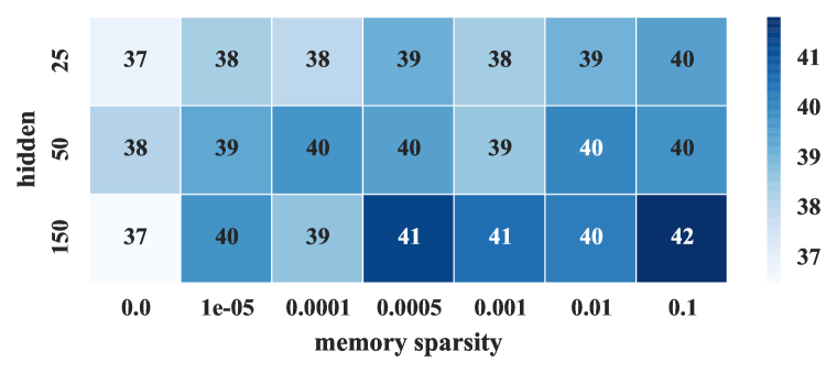
Figure 2: SST Root Accuracy with varying LSTM hidden size and sparsity penalty $\lambda$

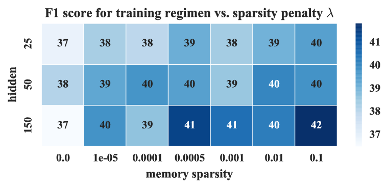
Figure 3: Effect of sparsity regimen and sparsity penalty $\lambda$ on SST Root Accuracy.

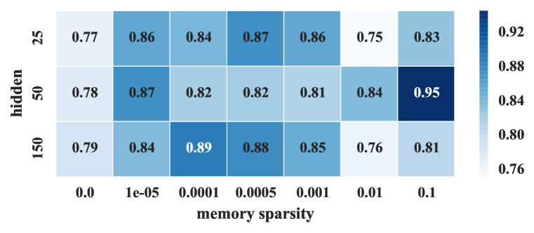
Figure 4: Paraphrase accuracy with varying LSTM hidden size and sparsity penalty $\lambda$

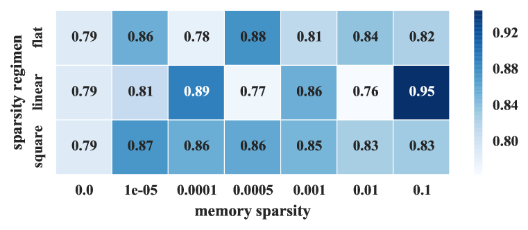
Figure 5: Effect of sparsity regimen and penalty $\lambda$ on Paraphrase prediction.

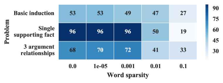
Figure 6: Accuracy for three bAbI tasks with varying $\lambda_{\mathrm{word}}$

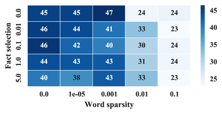
Figure 7: Effect of $\lambda_{\mathrm{word}}$ and $\lambda_{\mathrm{word}}$ on Basic Induction task accuracy

Table 2: Comparison of test accuracy on bAbI dataset from [27] with different models. Models are (left to right): LSTM baseline from [27], followed HG-LSTM with: no penalty, word sparsity penalty only, fact selection penalty only and both. The last column is MemNN.

task	LSTM	No penalty	Word Penalty	Fact Penalty	Fact, word	MemNN
single supporting fact	50	81	45	100	99	100
two supporting facts	20	32	19	30	32	100
three supporting facts	20	19	20	16	20	100
two arg relations	61	76	65	76	77	100
three arg relations	70	51	66	40	31	98
yes-no questions	48	48	51	50	50	100
counting	49	76	65	69	70	85
lists sets	45	78	66	76	73	91
simple negation	64	67	65	70	69	100
indefinite knowledge	44	45	47	40	44	98
basic-coreference	72	87	50	88	89	100
conjunction	74	75	66	99	99	100
compound-coreference	94	73	93	91	86	100
time reasoning	27	27	19	18	18	99
basic deduction	21	39	50	24	50	100
basic induction	23	44	42	47	40	100
positional reasoning	51	52	52	52	58	65
size reasoning	52	54	90	89	50	95
path finding	8	8	8	8	8	36
agents motivations	91	95	63	66	96	100

6.2 Interpretability

Ability to interpret the calculation carried out by Machine Learning models is crucial for advancing research. Especially for Neural Network models there are no well established methods for understanding its capabilities, although attempts have been made, e.g Hinton Diagrams [33]. We claim that Occam’s Razors provide some insights into the way network operates on it’s hidden state.

6.2.1 Error analysis

Diagnosing and identifying the root cause of errors during model design is critical for finding with new research directions and making improvements. We believe using Occam’s gates can help researchers gain insight into their network’s workings. To support this claim let us consider an example from bAbi dataset where gates provide a visual indication of progress.

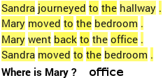
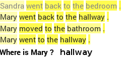
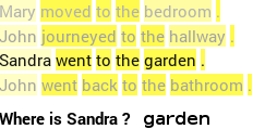
Figure 8: Example story from the single supporting fact bAbI. Activation of word gates is shown with yellow highlighter. Text opacity reflects the activation of the fact gate for the sentence. The images were taken when validation accuracy was 20%, 60% and 100% (left to right).

In Figure 8 we notice that the model upon reaching a validation accuracy of 20% is not yet capable of distinguishing important information from noise. At 60% accuracy it can now highlights the relevant facts, but the gates on words are not yet compelling. At 100% accuracy fact and word gates work in unison: the network activates for fact with the relevant person and words that contain location information. We hypothesize that LSTMs without gates can pick out the correct person and place, but Occam’s gates help them ignore facts about persons irrelevant to the question.

6.2.2 Relevancy detection

We argue that Occam’s gates allow one to judge which pieces of information are relevant to a problem. To illustrate this claim we show two examples, both of which emerged when training the system on a paraphrase detection problem with a Character model Gated LSTM (Char Gated LSTM). Figure 9 supports the belief that the model makes use word boundaries, and figure 10 suggests that the network can ignore repetititve or superfluous characters.

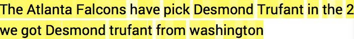
Figure 9: Char Gated LSTM, gate action shown with yellow highlighter. Model discovers tokenisation.

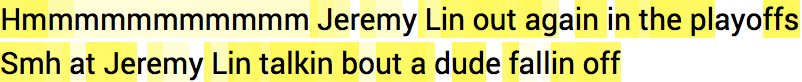
Figure 10: Char Gated LSTM, gate action shown with yellow highlighter. Model focuses on upper case characters and ignores repeats.

7 Conclusion

In this paper, we investigated the use of a complimentary objective function that forces attention-based RNNs to be selective about their inputs. We showed on three different tasks that our approach improves generalization and interpretability of the trained models with respect their counterparts that do not use sparsity penalties. Additionally, to encourage early exploration and preserve sparsity, we designed an annealing objective function that provides benefits over a standard one.

Finally, we introduced Hierarchical-Gated LSTM, a new model that performs significantly better than regular Stacked LSTMs; this network combines attentional and hierarchical components, and reasons at several levels of abstraction. Future work includes investigation of this model family, which shows promise towards advancing the state of the art.

References

References

- [1] Andrej Karpathy and Li Fei-Fei. Deep visual-semantic alignments for generating image descriptions. arXiv preprint arXiv:1412.2306, 2014.
- [2] Oriol Vinyals, Alexander Toshev, Samy Bengio, and Dumitru Erhan. Show and tell: A neural image caption generator. arXiv preprint arXiv:1411.4555, 2014.
- [3] Volodymyr Mnih, Nicolas Heess, Alex Graves, et al. Recurrent models of visual attention. In Advances in Neural Information Processing Systems, pages 2204–2212, 2014.
- [4] Karol Gregor, Ivo Danihelka, Alex Graves, and Daan Wierstra. Draw: A recurrent neural network for image generation. arXiv preprint arXiv:1502.04623, 2015.
- [5] Alex Graves. Generating sequences with recurrent neural networks. arXiv preprint arXiv:1308.0850, 2013.
- [6] Dzmitry Bahdanau, Kyunghyun Cho, and Yoshua Bengio. Neural machine translation by jointly learning to align and translate. arXiv preprint arXiv:1409.0473, 2014.
- [7] Jan Chorowski, Dzmitry Bahdanau, Kyunghyun Cho, and Yoshua Bengio. End-to-end continuous speech recognition using attention-based recurrent nn: First results. arXiv preprint arXiv:1412.1602, 2014.
- [8] Alex Graves, Greg Wayne, and Ivo Danihelka. Neural turing machines. arXiv preprint arXiv:1410.5401, 2014.
- [9] Wojciech Zaremba and Ilya Sutskever. Reinforcement learning neural turing machines. arXiv preprint arXiv:1505.00521, 2015.
- [10] Yin Zheng, Richard S Zemel, Yu-Jin Zhang, and Hugo Larochelle. A neural autoregressive approach to attention-based recognition. International Journal of Computer Vision, pages 1–13, 2014.
- [11] Nitish Srivastava. Improving neural networks with dropout. PhD thesis, University of Toronto, 2013.
- [12] Wojciech Zaremba, Ilya Sutskever, and Oriol Vinyals. Recurrent neural network regularization. arXiv preprint arXiv:1409.2329, 2014.
- [13] Vu Pham, Théodore Bluche, Christopher Kermorvant, and Jérôme Louradour. Dropout improves recurrent neural networks for handwriting recognition. arXiv preprint arXiv:1312.4569, 2013.
- [14] Justin Bayer, Christian Osendorfer, Daniela Korhammer, Nutan Chen, Sebastian Urban, and Patrick van der Smagt. On fast dropout and its applicability to recurrent networks. arXiv preprint arXiv:1311.0701, 2013.
- [15] Yichuan Tang, Nitish Srivastava, and Ruslan R Salakhutdinov. Learning generative models with visual attention. In Z. Ghahramani, M. Welling, C. Cortes, N.D. Lawrence, and K.Q. Weinberger, editors, Advances in Neural Information Processing Systems 27, pages 1808–1816. Curran Associates, Inc., 2014.
- [16] Jason Weston, Sumit Chopra, and Antoine Bordes. Memory networks. CoRR, abs/1410.3916, 2014.
- [17] Sainbayar Sukhbaatar, Arthur Szlam, Jason Weston, and Rob Fergus. Weakly supervised memory networks. CoRR, abs/1503.08895, 2015.
- [18] George Saon, Hong-Kwang J Kuo, Steven Rennie, and Michael Picheny. The ibm 2015 english conversational telephone speech recognition system. arXiv preprint arXiv:1505.05899, 2015.
- [19] Ilya Sutskever, Oriol Vinyals, and Quoc VV Le. Sequence to sequence learning with neural networks. In Advances in Neural Information Processing Systems, pages 3104–3112, 2014.
- [20] Wojciech Zaremba and Ilya Sutskever. Learning to execute. arXiv preprint arXiv:1410.4615, 2014.
- [21] Junyoung Chung, Caglar Gulcehre, Kyunghyun Cho, and Yoshua Bengio. Gated feedback recurrent neural networks. arXiv preprint arXiv:1502.02367, 2015.
- [22] Oriol Vinyals, Lukasz Kaiser, Terry Koo, Slav Petrov, Ilya Sutskever, and Geoffrey Hinton. Grammar as a foreign language. arXiv preprint arXiv:1412.7449, 2014.
- [23] Chris Dyer, Miguel Ballesteros, Wang Ling, Austin Matthews, and Noah A. Smith. Transition-based dependency parsing with stack long short-term memory. CoRR, abs/1505.08075, 2015.
- [24] Richard Socher, Alex Perelygin, Jean Y Wu, Jason Chuang, Christopher D Manning, Andrew Y Ng, and Christopher Potts. Recursive deep models for semantic compositionality over a sentiment treebank. In Proceedings of the conference on empirical methods in natural language processing (EMNLP), volume 1631, page 1642. Citeseer, 2013.
- [25] Marco Marelli, Luisa Bentivogli, Marco Baroni, Raffaella Bernardi, Stefano Menini, and Roberto Zamparelli. Semeval-2014 task 1: Evaluation of compositional distributional semantic models on full sentences through semantic relatedness and textual entailment. SemEval-2014, 2014.
- [26] Anthony Fader, Luke S Zettlemoyer, and Oren Etzioni. Paraphrase-driven learning for open question answering. In ACL (1), pages 1608–1618. Citeseer, 2013.
- [27] Jason Weston, Antoine Bordes, Sumit Chopra, and Tomas Mikolov. Towards AI-complete question answering: A set of prerequisite toy tasks. CoRR, abs/1502.05698, 2015.
- [28] Sepp Hochreiter and Jürgen Schmidhuber. Long short-term memory. Neural computation, 9(8):1735–1780, 1997.
- [29] Razvan Pascanu, Tomas Mikolov, and Yoshua Bengio. On the difficulty of training recurrent neural networks. arXiv preprint arXiv:1211.5063, 2012.
- [30] Klaus Greff, Rupesh Kumar Srivastava, Jan Koutník, Bas R. Steunebrink, and Jürgen Schmidhuber. LSTM: A search space odyssey. CoRR, abs/1503.04069, 2015.
- [31] Alex Graves and Jürgen Schmidhuber. Framewise phoneme classification with bidirectional lstm and other neural network architectures. Neural Networks, 18(5):602–610, 2005.
- [32] Matthew D Zeiler. Adadelta: an adaptive learning rate method. arXiv preprint arXiv:1212.5701, 2012.
- [33] Frederick J Bremner, Stephen J Gotts, and Dina L Denham. Hinton diagrams: Viewing connection strengths in neural networks. Behavior Research Methods, Instruments, & Computers, 26(2):215–218, 1994.