A stellar photo-polarimeter

Abstract

A new astronomical photo-polarimeter that can measure linear polarization of point sources simultaneously in three spectral bands was designed and built in the Institute. The polarimeter has a Calcite beam-displacement prism as the analyzer. The ordinary and extra-ordinary emerging beams in each spectral band are quasi-simultaneously detected by the same photomultiplier by using a high speed rotating chopper. The effective chopping frequency can be set to as high as 200 Hz. A rotating superachromatic Pancharatnam halfwave plate is used to modulate the light incident on the analyzer. The spectral bands are isolated using appropriate dichroic and glass filters.

A detailed analysis shows that the reduction of 50% in the efficiency of the polarimeter because of the fact that the intensities of the two beams are measured alternately is partly compensated by the reduced time to be spent on the observation of the sky background. The use of a beam-displacement prism as the analyzer completely removes the polarization of background skylight, which is a major source of error during moonlit nights, especially, in the case of faint stars.

The field trials that were carried out by observing several polarized and unpolarized stars show a very high mechanical stability for the polarimeter. The position angle of polarization produced by the Glan-Taylor prism in the light path is found to be slightly wavelength-dependent, indicating that the fixed super-achromatic halfwave plate in the beam does not fully compensate for the variation in the position angle of the effective optical axis of the rotating plate. However, the total amplitude of variation in the $U-I$ spectral region is only 0.^∘92. The polarization efficiency is also found to be wavelength-dependent with a total amplitude of 0.271% in the $U-I$ region; its mean value is 99.211%. The instrumental polarization is found to be very low. It is nearly constant in the $V-I$ spectral region ($\sim$ 0.04%), and apparently, it increases slightly towards the ultraviolet. The observations of polarized stars show that the agreement between the measured polarization values and those available in the literature to be excellent.

• Keywords : instrumentation: polarimeters – techniques: polarimetric – methods: observational, data analysis

1 Introduction

The linear polarization observed in stars, in general, is very small. A polarization of 0.01 (1 per cent) is considered to be quite large by the usual standards. It is essential that a high precision is achieved in polarimetry if the measurements of stellar polarization and attempts to detect any likely variation in it are to be meaningful. In principle, it is possible to attain a very high precision in polarimetry when compared to photometry since the former essentially uses the technique of differential photometry: we do not express the results in terms of the polarized flux, but in terms of the degree of polarization where the mean brightness of the star itself serves as the reference light level. This procedure eliminates to a large extent the adverse effects of atmospheric scintillation, seeing and transparency variation, the factors which usually limit the photometric accuracy. While achieving an external photometric consistency of 1 per cent is quite difficult even for bright objects, with suitable instrumentation and proper care it is possible to obtain an external consistency of 0.01 per cent in polarimetry, if sufficient photons are available.

There are several physical mechanisms that produce polarization of light from astronomical objects (Serkowski 1974b; Scarrott 1991). One of the most common processes that give rise to linear polarization of starlight involves circumstellar dust grains; they produce a net polarization in starlight integrated over the stellar disc either by scattering in an asymmetric envelope or by selective dichroic extinction. Measurements of polarization in multibands are required to study the nature of grains and their formation in the circumstellar environments. The observed polarization, in general, will contain a contribution from the interstellar dust grains, which could be quite significant in some cases. With reasonable assumptions about the interstellar component, it is possible to derive the intrinsic polarization exhibited by starlight if the wavelength dependence of the observed polarization is known. Polarimetric observations of Vega-like stars indicate that most of them show intrinsic polarization probably arising from scattering by dust grains confined to circumstellar discs (Bhatt & Manoj 2000). In order to improve the sample of such stars, ‘it is essential that the polarimeter should be able to measure polarizations which are extremely low ($<$ 0.1 per cent) because the material that constitutes the circumstellar discs is expected to be very tenuous. The observations done at Vainu Bappu Observatory during the past several years indicate that in some of the RV Tauri stars circumstellar grains either condense, or get aligned cyclically during each pulsational cycle, possibly triggered by the periodic passage of atmospheric shocks (Raveendran 1999a). In order to look for a possible evolution in the grain size distribution, in case it is the dust condensation that occurs, multiband observations are absolutely essential. Similarly, the identification of the polarigenic mechanism in T Tauri objects, which again constitute another group of objects extensively studied at the Institute (Mekkaden 1998, 1999), also requires a knowledge of the wavelength dependence of polarization. Some of the other polarimetrically interesting objects that are studied in the Institute using multi-spectral band data are Herbig Ae/Be stars (Ashok et al. 1999), Luminous Blue variables (Parthasarathy, Jain & Bhatt 2000), Young Stellar Objects (Manoj, Maheswar, & Bhatt 2002) and R CrB stars (Kameswara Rao & Raveendran 1993).

There was a need for an efficient photo-polarimeter for observations with the 1-m Carl Zeiss Telescope at Vainu Bappu Observatory, Kavalur. The star–sky chopping polarimeter, which was built by Jain & Srinivasulu (1991) almost a quarter century ago, was the only available instrument for polarimetric studies at the Observatory for several ongoing programmes. It is a very inefficient instrument. It uses a rotating HNP’B sheet as the analyzer and observations can be done only in one spectral band at a time. Further, the time spent on sky observations is always the same as that spent on star observations, irrespective of the relative brightnesses of the star and the sky background, and thus underutilizing the available telescope time.

A project to build a new photo-polarimeter for observations of point sources in $UBVRI$ bands with the 1-m telescope was initiated in the Indian Institute of Astrophysics quite sometime back. Unfortunately, due to unforeseen reasons there were delays at various stages of the execution of the project.

In this write-up we give the details of the three band, two beam photo-polarimeter for point sources that we designed and built in the Institute. In section 2 we give the working principle of the instrument. The optical layout, and the functions and details of important components are described in section 3. Several factors that have gone into the selection of the optical elements and the design of the various mechanical parts are briefly described in that section. The responses of the dichroic mirrors and the glass filters supplied by the manufacturer, and the mean wavelengths of the $UBVRI$ passbands of the polarimeter computed from the responses of the various components including the detector are also presented in the same section. A brief description of the polarized light in terms of the Stokes parameters and the effects of polarizer and retarders on these parameters when introduced in the light path are presented in the next section.

In section 5 we describe the various schemes of determination of linear polarization included in the reduction program, and discuss how the available time should be optimally distributed between the observations of object and background brightness in order to minimize the error in the linear polarization. A brief description of the electronics system that controls the polarimeter operations and data acquisition are given in section 6. The data reduction and display program is briefly described in section 7.

The polarimeter was mounted onto the 1-m Carl Zeiss telescope at Kavalur and observations of several polarized and unpolarized stars were made during 14 April–30 May 2014 to evaluate its performance. Due to prevalent poor sky conditions, the instrument could be used effectively only on a few nights during this period. The instrument was found to have a very high degree of mechanical stability, but a comparatively low polarization efficiency of 94.72%. In order to reduce the scattered light inside the instrument, we blackened the few internal mechanical parts that were left out earlier and improved light shields, and again made observations during February–April 2015; in section 8 we present a detailed analysis of these observations and the results obtained.

2 Principle of operation

The working principle of the polarimeter is illustrated in Figure 1. An astronomical polarimeter based on this principle was first built by Piirola (1973). A beam displacement prism divides the incident light into two beams with mutually perpendicular planes of polarization. The ordinary-beam, with the plane of polarization perpendicular to the plane containing the optical axis and the incident beam, obeys the Snell’s law of refraction at the prism surface and travels along the initial ray direction. The extraordinary-beam with vibrations lying in the

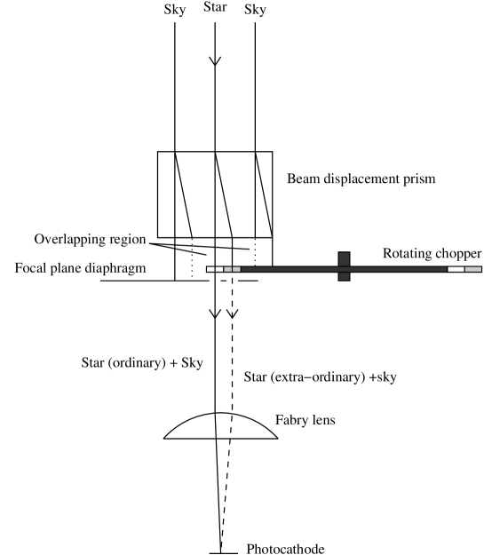
Figure 1: Working principle of the polarimeter.

above plane does not obey Snell’s law, and hence, travels in the prism with a speed that varies with the direction. As a result of these, the incident light beam will emerge from the prism as two spatially separated beams. The background sky, which acts as an extended object, illuminates the entire top surface of the beam displacement prism, and hence, produces two broad emergent beams whose centres are spatially separated by the same amount as above. There will be a considerable overlap between these two beams about the geometrical axis of the prism, and wherever the beams overlap in the focal plane of the telescope that portion remains unpolarized by the prism and observations give the background sky brightness directly. The situation is different with respect to the starlight; the star being a point source, there will be no overlap between the two emergent beams from the prism. The net result of these two effects is that we observe two images of the star with mutually perpendicular planes of polarization at the focal plane superposed on the unpolarized background sky. Two identical apertures are used to isolate these images, and a rotating chopper is used to alternately block one of the images allowing the other to be detected by the same photomultiplier tube.

The main advantages of such an arrangement are: (i) The contribution of background sky polarization is completely eliminated from the data, thereby, facilitating the observations of fainter stars during moonlit nights without compromising on the accuracy that is achievable during dark nights. This is possible because the background sky is not modulated, it just appears as a constant term that can be removed from the data accurately. (ii) Since the same photomultiplier tube is used to detect both the beams, the effect of any time-dependent variations in its sensitivity as a result of variations in the associated electronics, like, high voltage supply, is negligible. (iii) The quasi-simultaneous detection of both the beams using a fast rotating chopper essentially eliminates the effects of variations in sky-transparency and reduces the errors due to atmospheric scintillation for bright stars significantly. Scintillation noise is independent of the brightness of the star and dominates the photon noise for bright objects; with a 1-m telescope the low frequency ($<$ 50 Hz) scintillation noise is expected to be larger than the photon noise for stars brighter than B $=$ 7.0 mag at an airmass 1.0 (Young 1967). The averaging of the data by the process of long integration will reduce the scintillation noise only to a certain extent because of its log-normal distribution. The frequency spectrum of scintillation noise is flat up to about 50 Hz; the noise amplitude decreases rapidly above this frequency and it becomes negligibly small above 250 Hz. With the fast chopping of the beams and automatic removal of the background sky polarization it is possible to make polarization measurements that are essentially photon-noise limited.

The two factors that determine the overall efficiency of a polarimeter attached to a telescope are: (i) the faintest magnitude that could be reached with a specified accuracy in a given time, and (ii) the maximum amount of information on wavelength dependence that could be obtained during the same time. It is evident that the former depends on the efficiency in the utilization of photons collected by the telescope and the latter on the number of spectral bands that are simultaneously available for observation. In the beam displacement prism-based polarimeters, where the image separation is small, the intensities of the two beams produced by the analyzer are measured alternately using the same detector, and hence, only 50 per cent of the light collected by the telescope is effectively utilized. In polarimeters using Wollaston prism as the analyzer, the two beams, which are well-separated without any overlap, can be detected simultaneously by two independent photomultiplier tubes, fully utilizing the light collected (Magalhaes, Benedetti & Roland 1984; Deshpande et al. 1985). For simultaneous multi-spectral band observations that make use of the incident light fully, the beams emerging from the analyzer will have to be well-separated so as to accommodate a large number of photomultiplier tubes, making the resulting instrument both heavy and large in size (Serkowski, Mathewson & Ford 1975), and hence, not suitable for the 1-m telescope. Usually, in Wollaston and Foster prism-based polarimeters, when multispectral bands are available simultaneously, different spectral bands are distributed among the two emergent beams and at a time only 50 per cent of the light collected in each spectral region is made use of (Kikuchi 1988; Hough, Peacock & Bailey 1991).

Separate observations are needed to remove the background sky polarization when there is no overlap between the emergent beams, and a significant fraction of the time spent on object integration will have to be spent for such observations if the objects are faint. In beam displacement prism based polarimeters, time has to be spent only to determine the brightness of the background sky, and for the maximum signal-to-noise ratio it is only a negligible fraction of the object integration time even for relatively faint objects; the available time for observation can be almost entirely utilized to observe the object. Therefore, the non-utilization of 50 per cent light in beam displacement prism based polarimeters does not effectively reduce their efficiency, especially, while observing faint objects where the photons lost actually matter. The provisions for multi-spectral band observations can be easily incorporated in the design, making beam displacement prism based polarimeters to have an overall efficiency significantly higher than that of the usual Wollaston or Foster prism based polarimeters (Magalhaes, Benedetti & Roland 1984; Deshpande et al. 1985; Hough, Peacock & Bailey 1991). Another advantage of these polarimeters is that they can be easily converted into conventional photometers, just by pulling the beam displacement prism out of the light path.

3 The instrument

We adopted a design based on the beam displacement prism for the polarimeter because with such an instrument polarimetry can be done without compromising much on the precision even under moderate variations in background sky brightness and atmospheric transparency. The brightness in the blue spectral band, when the sky is dark, is about 15 mag, typically, if a focal plane diaphragm of 20 $arcsec$ diameter is used for observation. The background brightness continuously increases for a few hours after moon-rise and decreases for a few hours before moon-set. Even when the moon is high up in the sky the background brightness can change appreciably during the observation if the object integration lasts several minutes. Large changes in the background brightness can also occur if the sky is partially cloudy and moonlit. When Wollaston prism-based polarimeters are used an exact removal of the background polarization, which could be several tens of percentage, is extremely difficult. Sometimes, it may be even impossible to remove the background polarized flux accurately, if large changes occur in it. These instruments are effective in observing faint objects during dark periods of nights. But, with a beam displacement prism-based polarimeter reliable results can be obtained during fairly bright moonlit periods even when the sky is partially cloudy. In fact, most of the spectroscopic nights can be utilized for polarimetric observations with such an instrument. In the present polarimeter observations can be made simultaneously in three spectral bands. More sophisticated versions of the beam displacement prism are available elsewhere (Magalhaes & Velloso 1988; Scaltriti et al. 1989; Schwarz & Piirola 1999).

Figure 2: A schematic layout of the polarimeter indicating its main components.

The layout of the polarimeter indicating the positions of the main components is shown schematically in Figure 2.

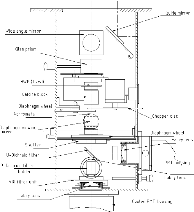
Figure 3: Schematic front-view of the polarimeter.

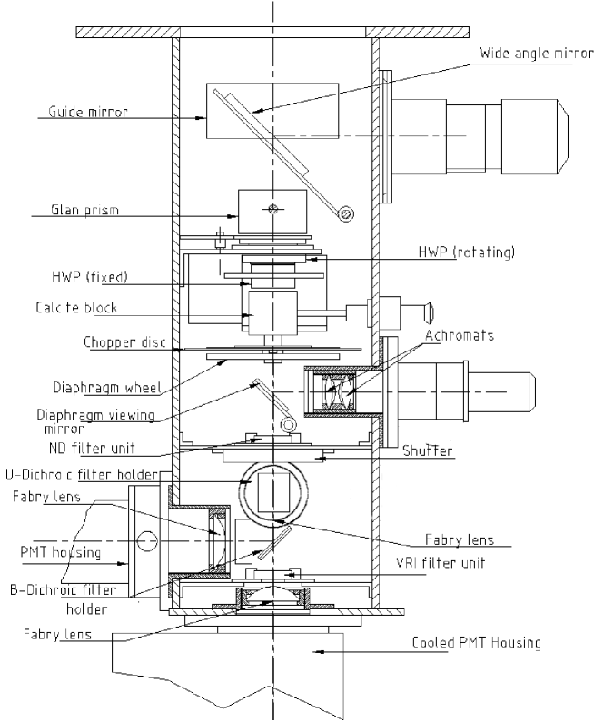
Figure 4: Schematic side-view of the polarimeter.

The front and side views of the polarimeter are schematically shown in Figures 3 and 4, indicating the important components. In the following subsections we describe the various components and the details which have gone into either their design, or their selection. The instrument was designed basically for use at the 1-m Carl Zeiss telescope of Vainu Bappu Observatory, as mentioned earlier; in principle, it can be used with any telescope having an f/13 beam with suitable modifications in the sizes of the twin diaphragms.

3.1 Wide angle viewing

The first element in the polarimeter is the wide angle viewing arrangement for object field identification. The star field is brought into the field of view of the eyepiece by flipping a plane mirror to a 45-degree position with respect to the telescope axis. The costs of the optical elements, like, half-wave plate and beam displacement prism, go up drastically with increase in their clear apertures. The Glan prism, which is used to calibrate the instrument for 100 per cent polarization, has a constant aperture-to-thickness ratio, and hence, larger the aperture, larger is its thickness. Since no re-imaging is done the diameter of the light beam produced by the telescope increases linearly with distance on either side of the image-isolating, focal plane diaphragms. In order to keep their clear apertures as small as possible, all the optical elements should be kept as close to the diaphragm as possible. The minimum distance between the centre of the wide angle mirror and the diaphragm, which could be accomplished, is 195 $mm$. At this distance the diameter of the F/13 beam is 15 $mm$. Assuming a field-stop of 50 $mm$ for a 2-$in$ barrel eyepiece (the maximum field-stop possible for such an eyepiece is 46 $mm$) the minimum width of the mirror should be 65 $mm$ and its length should be 92 $mm$. Since the mirror is introduced in a converging beam rather than a parallel beam, the centre of the mirror should be offset by about 1.5 $mm$, along the length of the mirror towards the side closer to the telescope back-end. We have used a 70 $mm$ $\times$ 100 $mm$ mirror. Because it is slightly oversized the mirror need not be offset to accommodate all the light collected by the telescope over the field. The flat mirror blank is made of borosilicate crown and an overcoating of silicon monoxide is given to protect the reflective aluminium coating for longer life.

For the object identification a field of view of about 10 $arcmin$ diameter is needed; this requires eyepieces of fairly long focal lengths with large field stops. Several makes of eyepieces with focal lengths around 50 $mm$ are available in the market. Gordon (1988), who made a comparative study of the performance of these eyepieces, has reported that the 4-element super Plossl eyepiece of 56 $mm$ focal length made by Meade has the best overall performance. The exit pupil, the image of the primary formed by the eyepiece, has a size of 4.3 $mm$. The eye-relief, which is the distance between the last physical element of the eyepiece and the exit pupil, is excellent ($>$ 38 $mm$). The eyepiece, like other makes of similar focal lengths, is not parfocal with other eyepieces, and hence, refocusing is needed if the eyepiece has to be replaced with another one of a different focal length. It has the largest apparent field of 52 degree among the eyepieces investigated by Gordon, and since a larger apparent field implies a higher magnification it also has the highest magnification. The apparent field of an eyepiece is the angle subtended at the eye by the circular patch that appears to the eye when viewed through it. The outer boundary is defined by the field stop, a metal ring that gives a sharp boundary by restricting the observer from seeing too far off axis, where the quality of star images becomes poor. The diameter of the field stop is approximately 46 $mm$. With an image scale of 15.5 $arcsec$ per $mm$ at the focal plane of the 1-m telescope the true field that can be viewed is about 12 $arcmin$, which is fairly good for object identification.

The axis of the field-viewing eyepiece is 100 $mm$ from the top of the mounting flange. With the position angle device, which has a thickness of 50 $mm$, there is sufficient clearance between the observer’s head and the back-end of the telescope, making the wide angle viewing convenient.

3.2 Offset guiding

Because of the diffraction phenomenon occurring at its aperture the starlight collected by a telescope will be distributed spatially in the image plane with the intensity falling off asymptotically as $r^{-3}$, where $r$ is the radial distance from the central axis. The reflector telescopes usually have a central obscuration, and for a typical Ritchie-Chretien telescope it is about 40 per cent of the full aperture. Figure 5 shows the intensity distribution due to diffraction effects at the focal plane of a 1-m telescope with and without the central obscuration. It also shows the energy excluded as a function of the diaphragm radius for both the cases. The main effect of the central obscuration is the redistribution of intensity in the outer rings, and thereby, spreading out farther the light collected by the telescope. It is clear from the figure that even with an aperture of 16-$arcsec$ diameter at the focal plane of a 1-m Cassegrain telescope the excluded energy is more than 0.5 per cent. If the aperture is not exactly at the focal plane the excluded energy will be significantly larger than the above (Young 1970).

The actual measurements of light lost in the focal plane diaphragm by Kron & Gordon (1958) show that the excluded energy can be several times larger than that indicated in Figure 5, where only the effects due to the classical diffraction phenomenon are included. The increase in excluded energy in practice arises from the extended rings of the star image primarily caused by the surface roughness of the telescope mirrors or the presence of dust on them (Kormendy 1973; Young et al. 1991).

If the star trails inside the diaphragm due to a poor tracking of the telescope, the included light will vary because the light thrown out on one side of the diaphragm will not be the same as that brought in on the other side of the diaphragm, thus, resulting in a variation in the output from the photomultiplier tube. The two images formed by the beam displacement prism passes through different regions of the various optical elements, like, filters. The transmittance of the glass filters and the reflectivity of the dichroic mirrors, in general, will not be the same across their surfaces; a spatial drift in the images will cause a variation in the differential throughput of the beams. The accuracy in the polarimetric measurements primarily depends on the accuracy in the determination of the ratios of the intensities of the two beams over a full rotational cycle of the signal modulator. If the star images trail inside the diaphragms there will be additional modulations of the ratio of intensities of the two beams, contributing to the errors in the measurement. For precise polarimetry it is essential that the star image should not drift inside the diaphragm even by a minute fraction of its size while observation, emphasizing the importance of the availability of a proper guiding facility.

Figure 5: Intensity distribution and the excluded energy due to diffraction.

Accurate guiding is possible if the image scale available for guiding is similar to that used for observation, making offset guiding the best option. Another plane mirror, which is also inclined at an angle of 45 degree to the telescope axis, is provided to reflect the starlight to the right side of the polarimeter for the purpose of guiding. Using a separate mirror for a guide star ensures that the alignment of the wide angle viewing arrangement with respect to the diaphragm is not disturbed, and thereby, saving the trouble of re-aligning it every time either the instrument is mounted onto the telescope, or a new object is acquired for observation, and improving slightly the efficiency in the use of telescope time. The centre of the mirror is at a distance of 210 $mm$ from the focal plane diaphragm. The width of the plane mirror used is 70 $mm$, which gives a projected cross-section of 50 $mm$, and its length is 120 $mm$. The unvignetted field of the 1-m telescope is 40 $arcmin$. The central clearance of the mounting flange of the polarimeter has a diameter of 168 $mm$, corresponding to a slightly smaller unvignetted field of 38 $arcmin$. The positioning of the rectangular mirror with respect to the telescope axis and the circular clearance of the mounting flange defines a field of 18 $arcmin$ $\times$ 8 $arcmin$ for choosing a guide star.

A suitable X-Y stage which can hold an intensified CCD is yet to be finalized.

3.3 Glan-Taylor prism

In order to measure the degree of polarization of the incident light accurately it is essential that the instrument should not cause any depolarization; it should have an efficiency of 100 per cent as a polarizer, because a good analyzer has to be a good polarizer. The polarization efficiency of the instrument should be frequently measured to look for any malfunctioning, and the availability of a provision for doing so at the telescope is highly desirable. A fully plane polarized beam that is necessary for this purpose can be obtained by inserting the Glan-Taylor prism in the path of the starlight. The prism is made of calcite, and its entrance and exit faces are normal to the direction of light path. Its angle has been cut such that the O-ray is internally reflected and absorbed by the black mounting material within the prism housing. The two halves of the prism are separated by an airspace for greater ultraviolet transmission. The usable wavelength range of the prism is 300 to 2700 $nm$. The extinction ratio is less than $10^{-5}$ for the undeviated ray. The polarization effect is maintained in a field of view of 13 to 7.5 degree, but it is symmetrical about the normal to the incident surface only at one wavelength. The symmetric field of view decreases with increase in wavelength; at 1000 $nm$ the full field of view is about 4.5 degree, and hence, the prism is suitable for an F/13 beam where the convergence angle is 4.4 degree. The clear aperture of the prism used is 24.5 $mm$ and its length is 25 $mm$. The deviation of the extraordinary beam on emergence from its initial direction is less than 2 $arcmin$. The lateral shift caused in the image will be less than 15 $\mu m$, and a re-centring of the star image inside the diaphragm may not be necessary after the introduction of the prism in the light path. Because of its fairly large length, when the prism is inserted in the light path a re-focusing of the image will be needed. The image plane will be shifted down by about 8.2-mm from its normal position when the prism is introduced. Among the polarizing prisms that are usually employed, Glan-Taylor prisms have the lowest length to aperture ratio ($\sim$ 0.85).

3.4 Signal modulation

The intensity of light at different position angles, which is needed for the determination of the degree of polarization, may be measured either by rotating the analyzer, or by rotating the entire instrument about the telescope axis. Both the procedures are cumbersome and involve a large amount of overhead time at the expense of the actual observational time. The star image will have to be centred inside the diaphragm at each position of the instrument or the analyzer during the rotation as it is extremely difficult to align the axis of the instrument or the analyzer with the respective rotational axes. When the analyzer is rotated the plane of polarization of light incident on the photocathode changes. Since the sensitivities of a cathode for different planes of polarization are not same, the rotation of the analyzer would either cause spurious polarization, or increase the error in the measured polarization unless a depolarizer efficient over the entire wavelength region of observation is inserted after the analyzer. These problems can be avoided if a rotating half-wave plate is introduced in the light path for modulating the starlight. If the half-wave plate is rotated by an angle $\psi$, most of the disturbing instrumental effects, in particular, those caused by image motion on the photocathode will have modulations with $\psi$ and 2$\psi$ angles, while the linear polarization will have a modulation of 4$\psi$. This effectively reduces the risk of spurious polarization caused by the image motion. However, there will be an increase in the error of measurement depending on the amplitudes of modulation with angles $\psi$ and 2$\psi$. The retarder rotated should be extremely plane parallel and the rotational axis should be exactly aligned with the normal to its light-incident face.

The modulating half-wave plate should be placed in front of the optical components which isolate spectral regions for observations because the latter usually polarize light; it is ideal to have the half-wave plate as the first element in the optical path inside the polarimeter.

A half-wave retarder made of a single plate will act as the same only at a particular wavelength and on either side of this the retardance continuously changes. If we have to cover a wide spectral range, the retardance should change as little as possible over the entire range. Achromatic retarders are produced by combining two plates of different birefringent materials. For good achromatism the surfaces should be flat to $\lambda$/10 and plane parallel to about 1 $arcsec$. The pair of magnesium fluoride and quartz provides a good combination and the retardance of an achromatic half-wave plate made out of these materials does not deviate more than 45 degree from 180 degree over the spectral range 300–1000 $nm$. These materials are transparent over a wide spectral range and are hard, and hence, easy to polish with a high precision. A very high degree of achromatism, super-achromatism, over the above spectral range can be obtained by using a Pancharatnam retarder which consists of three achromatic retarders, each made by a combination of quartz and magnesium fluoride and operating in a particular wavelength region. Such a retarder was used for the first time in an astronomical polarimeter by Frecker & Serkowski (1976). The achromatic retarders, which form the superachromatic combination, are cemented to each other. The calculated path difference for such a superachromatic half-wave plate is plotted in the top panel of Figure 6. In the spectral range 310–1100 $nm$ the path difference (R) lies within $\pm$1.3 per cent of $\lambda$/2, and during the manufacture it is possible to achieve the theoretical retardation to an accuracy of about $\pm$3 per cent. The error introduced by this in the measurement of linear polarization will be almost non-existent (see section 4.4).

Figure 6: Calculated position angle of the effective optical axis and retardation for a superachromatic half-wave plate.

The main drawback of the Pancharatnam retarders is the wavelength dependence of position angle of their effective optical axis as seen in the bottom panel of Figure 6. Over the spectral region 310 to 1100 $nm$ the orientation of the expected effective optical axis on the surface rotates by about $\pm$2.5 degree; the actual range could be slightly larger than the theoretical value. This would cause difficulties in the accurate determination of the position angle of polarization when broad spectral bands, as in the present case, are used for observations because corrections that are to be applied to the position angles would depend on the energy distribution of the observed objects. Such an inconvenience can, fortunately, be avoided by introducing another stationary identical Pancharatnam plate immediately in the light path. The introduction of such a half-wave plate ensures that the signal modulation is only a function of the relative positions of the effective optical axis of the two half-wave plates. The stationary half-wave plate is mounted with its effective optical axis approximately parallel to the principal plane of the analyzer, which in this case is the calcite block mounted just below this. This is to reduce the contributions to the modulation of intensity of transmitted light from terms that depend on the sine of position angle of optical axis.

For a birefringent material the reflection coefficient even for normal incidence depends on the position angle of the plane of vibration, and hence unpolarized light may become polarized after passing through a retarder. To reduce the polarization by refraction, the six plates of the superachromatic half-wave plates are cemented with cover plates made from fused silica Suprasil, which is an isotropic material, and the outer surfaces are single-reflection coated. The two identical half-wave plates of 19-$mm$ clear aperture used in the polarimeter are acquired from Bernhard Halle Nachfl. GmbH, Berlin, Germany.

The half-wave plate is rotated using a stepper motor of Model No. MO61-FC02, procured from Superior Electric. It makes one rotation in 400 half-steps, and is coupled to the halfwave plate through a 1:1 anti-backlash spur gear system.

3.5 Calcite block

The role of the analyzer is performed by the calcite block introduced in the light path immediately after the stationary half-wave plate. The optical components, dichroic filters and diffraction grating, that are commonly used to isolate spectral regions in multichannel instruments change the state of polarization of the incident light, and hence, the analyzer should be placed in front of all such components.

As mentioned already the light beam splits into two at the incident surface of a beam-displacement prism. If the optical axis is parallel to the incident ray both beams travel with the same velocity inside the prism and if it is perpendicular they travel along the same direction with an ever increasing phase difference between them; in both cases the emergent beams produce a single image. When the optical axis makes any other angle with the incident ray the two beams travel in different directions and produce two spatially separated beams on emerging from the crystal. The maximum separation between the emergent beams occurs when the optical axis is inclined at an angle of 45 degree with the incident beam. Since the light beam is incident normal to its face, a beam displacement prism is cut with its optical axis making an angle of 45 degree with the incident face. The Huygens wave front of the ordinary vibrations is spherical while that of the extraordinary vibrations is an ellipsoid of revolution about the optical axis, with the major axis inclined at an angle of 45 degree to the incident beam, and this causes the splitting of the incident beam. If $\theta$ is the deviation of the extraordinary beam from the ordinary beam then

$$\tan\theta=\frac{n_{e}^{2}-n_{o}^{2}}{n_{e}^{2}+n_{o}^{2}}\,,$$

where $n_{e}$ and $n_{o}$ are the refractive indices of the extraordinary and ordinary rays. If $t$ is the thickness of the prism, the separation $d$ of the two beams on emerging from it will be

$$d=t\,\tan\theta.$$

It is clear from the above two relations that the separation between the images depends on the difference in the refractive indices of the ordinary and extraordinary rays. Of the commonly available crystals, quartz, magnesium fluoride, sapphire, calcite, KDP and lithium niobate, calcite has the largest difference between $n_{e}$ and $n_{o}$, and hence, for a given thickness a calcite plate gives the largest separation between the beams. Calcite is a negative crystal; at $\lambda$ = 589 $nm$, $n_{o}$ = 1.65835, $n_{e}-n_{o}$ = $-$0.17195, and the deviation of the extraordinary beam from the ordinary beam, $\theta$ = 6.22 degree. Since the difference in the refractive indices of the two beams is a function of wavelength, the spatial separation of the two beams also will be a function of wavelength. The separation as a function of wavelength expected for a calcite plate of 14 $mm$ thickness is plotted in Figure 7; the refractive indices needed for the computation are taken from Levi (1980).

Figure 7: Separation between the ordinary and extra-ordinary images produced by a single calcite plate.

The introduction of the calcite plate in the converging beam will shift the focal plane away from it. If $t$ is the thickness and $n$ the refractive index, the shift produced in the focal plane is given by

$$\Delta F\approx\frac{t}{n}\,(n-1).$$

With $t$ = 28 $mm$, at $\lambda$ = 589 $nm$, for the ordinary beam $\Delta F$ $\approx$ 11 $mm$. Because of the variations in the refractive index with wavelength even the ordinary image will show chromatic aberration. The extraordinary image will show astigmatism additionally because the corresponding beam propagates obliquely through the plate at an angle of about 6 degree with respect to the normal to the surface. The predominant aberrations shown by the image will be very similar in magnitude to those that would be produced by a beam of light passing through a glass plate at an angle same as above (Brand 1971). Consequently, the focal planes, planes containing the circle of least confusion, for the two beams will not be the same. Further, as a result of the Fresnel reflection losses from the surface being different for the two orthogonal planes of polarization the two beams will have slightly different intensities even for unpolarized objects. Both these inconvenient features of a single calcite plate can be avoided if two cemented plane parallel plates with their principal planes crossed at right angles are used (Serkowski 1974a); the light which is ordinary in the first plate becomes extraordinary, and vice versa in the second. Hence, both the images of a star produced by a calcite block with two crossed plates will be affected similarly and the images will have circles of least confusion in the same plane. This will enable one to obtain the same degree of focus for both the images inside the corresponding apertures.

Table 1: Parameters of the images formed by the calcite block.

Parameter	Value ($mm$)
Single calcite plate:
Separation of images at 320 $nm$	1.780
Separation of images at 990 $nm$	1.462
Length of the image strip	0.318
Mean offset of the image centre from the initial direction	1.621
Two crossed calcite plates:
Centre-to-centre distance of the two images	2.292
Offset of the centre of the images from the initial direction∗	1.146
* The calcite block is rotated such that the offset is towards the observer

We have used a 20-$mm$ clear aperture calcite block made of two cross-mounted plates of each 14-$mm$ thickness; this is also acquired from Bernhard Halle Nachfl. GmbH. The transmission of such a block over the spectral region 300–1000 $nm$ is close to 90 per cent (McCarthy 1967). The computed parameters of the images are given in Table 1. The calcite block is mounted such that the line joining the centres of the images is parallel to the front side of the polarimeter. It can be removed from the light path, if needed, to use the instrument as a three channel photometer with or without the star-sky chopping facility.

3.6 Diaphragms and image chopper

The maximum back focal length from the last mounting plate with the position angle device of the 1-m Carl Zeiss telescope at Kavalur is 324$~{}mm$. The diaphragms are placed at a distance of 295 $mm$ from the top of the mounting flange of the polarimeter, which is well within the allowed range. The details of the diaphragms that are available are given in Table 2. The disc on which these diaphragms are mounted is made to protrude slightly outside the instrument-body to facilitate its rotation manually for choosing the required set of twin diaphragms for observation. The centres of the twin diaphragms are aligned along the radial direction of the disc. They should always be accurately positioned at the same locations with respect to the axis of the instrument to avoid any change either in the angle of incidence on the photocathode or in the region of illumination on its surface by the two images. A possible light leak through the slot made on the side plate of the instrument is arrested by using a cap to the protruding portion. It is seen from from Figure 5 that the excluded energy is nearly flat beyond a radius of about 7 $arcsec$, and hence, with the 1.3-$mm$ diaphragm, which corresponds to an angular diameter of 20 $arcsec$, the excluded light is less than 0.5 per cent.

The 1.3-$mm$ single diaphragm is included for the purpose of using the instrument as a conventional photometer without star-sky chopping or as a polarimeter in single image mode. The 4.5-$mm$ single diaphragm is included for the purpose of field-viewing to make centring of the images inside the smaller diaphragms for observation easy. It is highly desirable if the metal focal plane diaphragms that are used currently are replaced with those made of a non-metallic material. Serkowski (1974a) has reported that when the star image was on the edge of a metallic diaphragm such that only about half of the light entered the polarimeter a linear polarization over 0.2 per cent with the position angle parallel to the edge of the diaphragm was found. Hence, if the star image drifts during the observation it could increase the errors in the polarization measurements significantly, if metallic apertures are used.

The twin diaphragms need not be of equal sizes if the instrument is used only in the double image mode polarimetry because the sky intensity in each beam is observed and removed separately. But, it is better to have identical diaphragms if the instrument has to be used in the star-sky chopping photometric mode; if they are of different sizes their relative sizes should be known exactly for the removal of the sky background.

Table 2: Details of the apertures available in the instrument.

Linear Diameter	Angular diameter	Nature
($mm$)	($arcsec$)
1.3	20	Twin
1.6	25	Twin
1.3	20	single
4.5	70	single

The annular opening on the chopper disc, which is meant for the alternate blocking of one of the images, has a width of 4 $mm$, and has been divided into four segments, two alternate ones for each image. The diameter of the disc is 158 $mm$ and that of the common boundary of the slots that isolate the images is 142 $mm$. The counting of the photomultiplier pulses should begin only when the corresponding diaphragm is fully open, which means that the counting should commence only when the chopper slot has advanced by the diaphragm size and the counting should end before the chopper starts obstructing the diaphragm. Further, the position sensors are about 2 $mm$ in size. The size of the slots in the chopper during the rotation of which the pulse counting is done subtends an angle of 82 degree at the centre; the 8-degree blind stretch ensures that counting is done only when the diaphragms are not blocked by the chopper. The observations can be made over close to 91 per cent of the rotation of the disc; probably, this can be increased marginally by reducing the blind sector a little. With a larger chopper disc the fractional size of the blind stretch can be reduced; but, because the alternate slots have a common boundary the blind stretch cannot be made very small either. The size of the body of the instrument would increase, and hence, also its weight, if we have to accommodate a larger disc. Even with the present size for the chopper disc a portion of it protrudes outside the body of the instrument; the protrusion is covered with a cap to avoid any accidental contact with the chopper while in rotation and to prevent the light leak through the slot on the side plate through which it protrudes. The top surface of the chopper disc is separated from that of the image-isolating apertures by slightly more than 3 $mm$. The centres of the apertures are horizontally at 1.146 $mm$ from the common boundary of the chopping slots. This corresponds to an angular distance of about 18 $arcsec$ from the axis of the telescope, and the fractional excluded energy by a diaphragm of this radius at the focal plane is about 0.2 per cent. When it is less than about 1 per cent, the excluded energy is not a sensitive function of the vertical distance from the focal plane for a fixed horizontal distance from the telescope axis (Young 1970). Therefore, the chopper does not increase the excluded energy even when the 1.6 $mm$ twins apertures are used.

The chopper disc is rotated directly by using a servo motor with the Model No. Smartmotor^® SM2315 procured from Animatics. The whole chopper unit can be finely aligned so that the common boundary of the slots that isolate the images bisects the line joining the centres of the twin apertures.

The line joining the centres of twin diaphragms is made parallel to the front side of the polarimeter. The diaphragm and the chopper discs are mounted on the two opposite side plates of the instrument.

The diaphragm viewing arrangement consists of a pair of achromats of focal length 93 $mm$ and aperture 30 $mm$ for re-imaging, and a Meade 3-element modified achromatic eyepiece of 12-$mm$ focal length. Both spherical and chromatic aberrations are reduced considerably by using twin achromats with similar elements facing each other while re-imaging. The eyepiece has a field of about 40 degree and a field stop of about 8 $mm$. The starlight is brought into the field of view of the achromats by flipping a flat mirror of size 40 $mm$ $\times$ 40 $mm$ to a 45 degree position. If the 4.5-$mm$ aperture has to viewed completely, the image formed by the achromats at the focal plane of the eyepiece should be less than its field stop. This requires that the magnification produced by the achromats should be less than 1.8. With a distance of 75 $mm$ between the apertures and the first achromat this can be achieved. The image formed by the second achromat will then be at a convenient distance of about 125 $mm$ from it.

3.7 Filters and detectors

If the objects to be observed could cause count rates in excess of their maximum values allowed by the upper limits on the anode currents, the incident light intensities should be cut down to avoid any damage to the photomultiplier tubes. For this purpose two neutral density filters of optical densities 1.0 and 2.0 are made available. Since the optical density is the base ten logarithm of opacity, which is simply the reciprocal of the transmittance, the above densities translate to 2.5 and 5.0 magnitudes, respectively. Both filters are of absorptive type, and hence, do not produce any scattered light when inserted in the light beam. The wavelength dependencies of these filters are plotted in Figure 8 which shows that these filters are not strictly neutral; the changes in the mean wavelengths of the spectral bands produced by these filters on inserting in the light path should be taken into account when the effective wavelengths of observation are computed, or when standard magnitudes of the programme objects are derived. These 30-$mm$ diameter circular filters are mounted on a sliding holder having an additional clear hole that allows the light to pass through unattenuated while observing objects which are within safe brightness limits. These neutral density filters would also be useful to cut down the brightness of objects by a known factor when observations are made to determine the dead-time coefficients of the pulse counting setup.

Figure 8: Wavelength dependence of the neutral density filters available.

Figure 9: Wavelength characteristics of the dichroic filters used.

The isolation of the spectral regions into the three channels of the polarimeter is achieved by using two dichroic filters, one to reflect the ultra-violet part of the incoming light and the other to reflect the blue part of the spectrum from the light transmitted by the first. The filters are mounted such that the two beams are reflected in mutually perpendicular directions, with the $U$ band on the right side of the instrument and the $B$ band behind; in this configuration the instrument becomes more compact. The dichroic filters used are obtained from Custom Scientific, Inc., Arizona, USA. The wavelength characteristics of these filters are given in Figure 9. The reflective coatings required for the dichroism are done on 2-$mm$ thick glass substrates. The calcite block and dichroic filters are mounted such that the vibrations of the two mutually perpendicularly polarized beams make an angle of 45 degree with the plane of incidence on the dichroic filters. This ensures that the reflectivity of both beams are the same, and hence, does not introduce any differential change in the intensities of the beams.

Figure 10: Transmission characteristics of the Schott glass filters used.

Figure 11: Combined spectral responses of the dichroic mirrors and glass filters.

The two reflected beams are detected by two separate uncooled photomultiplier tubes. The bi-alkali photocathodes of these tubes along with the Schott glass filters inserted in front of them produce spectral bands that approximate the $U$ and $B$ bands of Johnson. The light transmitted by both the dichroic filters, which fall in the $VRI$ spectral bands, is detected by a cooled photomultiplier tube with a GaAs photocathode. The observations are made sequentially in $V$, $R$ and $I$ bands using suitable filter combinations mounted on a sliding filter holder. These filters have clear apertures of 25-$mm$ diameter. The transmission characteristics of the Schott glass filters that are used are given in Figure 10. The combined responses of the dichroic mirrors and the glass filters are plotted in Figure 11 and the final band passes that include the detector quantum efficiencies are plotted in Figure 12. The $R$ and $I$ passbands approximate that of Cousins (Bessel 1979, 1993), while the $V$ passband approximates that of Johnson. The selection of required glass filters are based on the filter-detector combinations used by Piirola (1988) and Hough, Peacock & Bailey (1991); these authors also have employed dichroic filters to isolate spectral regions in their multiband polarimeters. The details of the filter-detector combinations used are given in Table 3. The mean wavelength, which is defined as

$$\lambda_{0}=\frac{\int\lambda\,S(\lambda)\,\delta\lambda}{\int S(\lambda)\,\delta\lambda},$$

calculated from the data is also given in the table against the corresponding spectral band; S($\lambda$) is the wavelength-dependent response plotted in Figure 12.

Table 3: Filter-detector combinations used in the instrument.

Spectral	Filter combinations	Mean wavelength	Photomultiplier tube
band		$\lambda_{0}$ ($nm$)
$U$	UG1 (1 $mm$)	357	ETL 9893Q/350B
$B$	BG12 (1 $mm$)	437	ETL 9893Q/350B
$V$	BG18 (1 $mm$) +	561	Hamamatsu R943-02
	GG495 (2 $mm$)
$R$	OG570 (2 $mm$) +	652	${}_{{}^{\prime\prime}}$
	KG3 (2 $mm$)
$I$	RG9 (3 $mm$)	801	${}_{{}^{\prime\prime}}$

Figure 12: Combined spectral responses of the filter-detector combination.

3.8 Fabry lenses

The photocathode should be located exactly at the exit pupil of the Fabry lens so that the image of the primary mirror on the cathode will be in good focus. If not, the two stellar images formed by the calcite block will not fall at the same spot on the cathode, and this will produce an appreciable difference in the corresponding signals from the photomultiplier because the sensitivity across the photocathode surface is not uniform. The two images of the primary on the cathode, in general, will not have the same brightnesses across them because the two beams take different paths through the various optical elements, and the surface inhomogeneities in the transmittance and reflectivity of these elements modify them differently; this will give rise to a difference in the signals even if the images fall at the same spot, the ratio of the net responses, however, will be a constant. The atmospheric scintillation also produces a distribution of brightness across the images, but the distributions will be the same since the air is birefringent. If the cathode is kept at a distance $\Delta F$ from the focus, the image-spots on the cathode will be separated by a distance $d$ given by (Serkowski & Chojnacki 1969)

$$d=\frac{x\,\Delta F}{F},$$

where $x$ is the linear separation between the images at the focal plane and $F$, the focal length of the Fabry lens. If $F_{ratio}$ is the focal ratio of the telescope, the size $s$ of the image is given by

$$s=\frac{F}{F_{ratio}}.$$

If $r$ is the ratio of the separation of images to the image size, then

$$r=\frac{x\,\Delta F}{s^{2}F_{ratio}},$$

indicating that a larger image of the primary would give a smaller value for $r$ and therefore a smaller effect due to an error in focusing. The maximum sizes that the images can be of are decided by the effective sizes of the cathodes. The cathodes of ETL 9893 and Hamamatsu R943-02 are of 9 $mm$$\times$ 9 $mm$ and 10 $mm$ $\times$ 10 $mm$, respectively. Normally, an image of diameter about half the size of the cathode is used.

Plano-convex lenses of 75-$mm$ focal length at 5876Å  are used in all the three channels. The lenses are made of synthetic fused silica, which is far purer than fused quartz. The increased purity makes fused silica to have excellent transmission from ultra-violet to infrared; in the optical region its transmission is about 5 per cent better than that of BK7. The focal length $F$ and radius of curvature $R_{c}$ of a plano-convex lens are connected according to the equation

$$\frac{1}{F}=\frac{\mu-1}{R_{c}},$$

where $\mu$ is the refractive index. Because of the wavelength-dependence of the refractive index the focal length, and hence, the size of the image formed on the cathode varies with wavelength. Table 4 gives the focal lengths and sizes of the images at a few selected wavelengths. The fractional size of the image with respect to the size of the cathode is also given in the table.

Table 4: Focal lengths of the Fabry and the sizes of the image formed.

Wavelength	Refractive index	Focal length	Image size	Fractional size of
($nm$)	$\mu$	($mm$)	($mm$)	the image (per cent)
351.1	1.47671	72.1	5.5	61
457.9	1.46498	73.9	5.7	63
546.1	1.46008	74.7	5.7	57
587.6	1.45846	75.0	5.8	58
643.8	1.45637	75.3	5.8	58
786.0	1.45356	75.8	5.8	58

The Fabry lenses used in the $U$ and $B$ channels can be focused properly. Since the same Fabry is used in the $VRI$ channel it is impossible to get a good focus in all the three bands simultaneously. Assuming that a good focus is obtained for the $R$ band, then the cathode will be away from the focal plane for the $V$ and $I$ bands by $\pm$0.6 $mm$. With a separation of 2.292 $mm$ between the centres of the two images at the focal plane of the telescope, the above corresponds to a separation of 18 $\mu$m between the centres of the corresponding image-spots on the cathode. The resulting ratio of the separation of image-spots to their size, $r\approx$ 0.3 per cent. To overcome the adverse effect of nonuniform sensitivity over the cathode surfaces the practical rule is that the relative shifts in the image of the primary mirror formed by the Fabry lens on the detector should not exceed 0.01 per cent of the diameter of the image (Serkowski 1974b). The relative separation of the images will give rise to a small difference in the output signal, but with a constant gain-ratio. This will not be a serious problem because the ratio of overall throughputs for the two beams can be treated as an unknown in the data reduction procedure. The images should remain at the same positions with respect to the cathode over a full rotation of the half-wave plate, which means that we should be able to keep the image drift inside the diaphragm below 2 $arcsec$ which corresponds to a value of $\sim$ 0.01 per cent for the ratio of drift in image-spots to their sizes, by accurately guiding the object. If the Fabry is in good focus, which can be achieved in principle for the $U$ and $B$ channels, then a drift of the images on the detector surface will not produce any significant effects in the results since the fast chopping rate between the images essentially ensures that the effective sensitivity is the same for both the beams. The problems associated with the nonuniform sensitivity of the cathode can be minimized if the images are formed at the most sensitive region of the cathode where the gradient of sensitivity is the least (Young et al. 1991). Since the position of maximum sensitivity does not usually coincide with the geometrical centre of the cathode such an alignment can be made only with extra difficulties.

The actual sizes of the images of the primary mirror formed on the cathodes will be slightly more than those given Table 4 because of spherical aberration. All the aberrations depend on the way a lens is used. The plano-convex Fabry lenses are mounted with their curved surfaces facing the primary mirror to reduce spherical aberration.

The longitudinal spherical aberration $a_{l}$, which is the distance along the optical axis between the intercepts of the paraxial and marginal rays, for a plano-convex lens of focal length $F$ with its convex surface facing the infinite conjugate is given by (Subrahmanyam 1980)

$$a_{l}=\frac{\rho^{2}\,(\mu^{3}-2\,\mu^{2}+2)}{2\,F\,\mu\,(\mu-1)^{2}},$$

where $\rho$ is the distance between the marginal rays and the optical axis, and $\mu$, the refractive index of the lens material. The distance from the axis at which the marginal rays meet the paraxial focal plane is the transverse spherical aberration, $a_{t}$, and it is given by

$$a_{t}=\frac{a_{l}\,\rho}{F-a_{l}}.$$

It is this aberration which increases the spot-size on the photocathode. The focal ratio at which the lens is operated is 2$\rho/F$, and it is clear from the above relations that the transverse spherical aberration increases with the focal ratio of the beam.

The lenses are about 220 $mm$ from the focal plane of the telescope, and hence, are operated approximately at $F$/3.6. At this $F$-ratio for the beam the increase in the image diameter due to transverse spherical aberration is about 0.5 $mm$.

3.9 PMT housings

As indicated earlier ETL 9893Q/350 photomultiplier tubes are used in the $U$ and $B$ channels; their quartz windows give extended ultra-violet response. These tubes have bi-alkali photocathodes with small effective diameters, and therefore produce very low dark counts; according to the manufacturer’s specification, at an ambient temperature of 20^∘ C the tubes give around 40 counts s^-1 when the cathode to anode voltage is 2250 V, and on cooling the counts will be reduced only by a factor of about two. Therefore, uncooled ambient housings (ETL B2F-type), which are used for the above channels mainly to reduce the size and total weight of the instrument, are sufficient for the purpose.

The Hamamatsu R943-02 tube used in the $VRI$ channel has a GaAs photocathode. At ambient temperatures these tubes give a few thousand dark counts per second under typical operating voltages. To reduce the dark counts we have used a FACT 50 model housing, which is of forced air-cooled type and cools 50^∘C below ambient air at 20^∘C with a cool down time of about 1.5 hours.

We have fitted all the three housings with individual shutter assemblies so that the housings can be dismantled from the main structure of the polarimeter without removing the photomultiplier tubes. These mechanical shutters can be kept open during the night because an electronically operated shutter, common to all the three photomultiplier tubes, is provided. This shutter is immediately after the neutral density filters in the light path and is operated during the observations. The plane of the window of the photomultiplier tube is set 10.2 $mm$ behind the top of the mounting flange of the B2F-type housing. In the case of ETL 9893 tubes the photocathode is just behind the window of the tube, and hence, there is sufficient space to accommodate a PR305 shutter assembly acquired from Electron Tubes Limited (ETL), which is about 22 $mm$ thick, between the photocathodes and the Fabry lenses. In the case of FACT 50 housing the window of photomultiplier tube is set about 32 $mm$ behind the face of the mounting flange. The cathode of R943-02 tube is 19 $mm$ behind its window. Since there is no space to accommodate a similar shutter in the $VRI$ beam, the mechanical assembly interfacing the housing to the polarimeter is designed to incorporate a shutter to control the light reaching the photomultiplier. An offset of 1.6 $mm$ of the photocathode centre from the axis of the R943-02 photomultiplier tube is taken care of by offsetting the centre of the bottom mounting plate of the instrument. The photomultiplier tube base is rotated such that the offset is in the right direction.

A well-focused Fabry lens while keeping the image-spot at the same position on the cathode transforms the spatial changes at the focal plane of telescope to changes in the incident angles on the cathode. The cathode of R943-02 is inclined at an angle of 15 degree with respect to the input window surface. The Fresnel reflection losses will be different for the two beams if their incident angles are different. The tube is mounted such that the axis about which the cathode is tilted is parallel to the line joining the two images. This makes the incident angles of both the beams on the cathode the same. If the star images drift inside the diaphragm, the incident angles may become different depending on the direction of drift on the cathode surface and may cause differential variation in the signal. This is true even for the ETL 9893 tubes where the photocathodes are parallel to the input window, though the associated problems will be less than that for the GaAs tube. To reduce the polarimetric errors it is necessary to keep the images at the same position inside diaphragm during the full rotation of the half-wave plate by accurate guiding.

4 Polarized light

The underlying principle in the measurement of polarization of a beam of light is that its state of polarization can be altered in a desired way by introducing appropriate optical elements in its path. In the present case it is the half-wave plates–calcite block combination that does the required modification. In order to know how a particular optical element affects the state of polarization, the most important requirement is a way of quantitative parametrization of the state of polarization of a beam of light. In the following subsections we briefly describe the parameters that are used to characterize a polarized beam of light and the effects of introducing the half-wave plates and calcite block in the path on the state of polarization of the incident light beam; the different possible states of polarization of a beam of light are also briefly discussed in the subsections that follow.

4.1 Stokes parameters

The state of polarization of a beam of light, particularly in scattering problems, is most conveniently described using the Stokes parameters (Van de Hulst 1957) which are defined as

$$I=E_{0x}^{2}+E_{0y}^{2},$$

$$Q=E_{0x}^{2}-E_{0y}^{2},$$

$$U=2\,E_{0x}\,E_{0y}\,\cos\delta\quad\mbox{and}$$

$$V=2\,E_{0x}\,E_{0y}\,\sin\delta,$$

where $E_{0x}$ and $E_{0y}$ are the amplitudes of the electric vector in two orthogonal planes $x-z$ and $y-z$, and $\delta$ is the phase difference between the $x-$ and $y-$vibrations; the instantaneous values of the electric vector are

$$E_{x}=E_{0x}\,\cos\omega t\quad\mbox{and}\quad E_{y}=E_{0y}\,\cos(\omega t+\delta).$$

We can define a vector $E_{0}$ whose amplitude is $(E_{ox}^{2}+E_{0y})^{\frac{1}{2}}$ and which makes an angle $\theta$ with the positive $x-$axis such that $E_{0x}=E_{0}\,\cos\theta$ and $E_{0y}=E_{0}\,\sin\theta$. Usually, the angle $\theta$ is called the position angle of polarization. $E_{0x}$ and $E_{oy}$ can take both positive and negative signs, defining the quadrant in which $\theta$ lies. The Stokes parameters can be re-written in terms of the position angle of polarization and the phase difference between the two orthogonal components of the electric vector as

$$I=E_{0}^{2},$$

$$Q=I\,\cos 2\,\theta,$$

$$U=I\,\sin 2\,\theta\,\cos\delta\quad\mbox{and}$$

$$V=I\,\sin 2\,\theta\,\sin\delta.$$

The most general form of polarization is elliptical polarization where the end points of the instantaneous electric vectors always lie on an ellipse; all the other states of polarization are its special cases. It is clear that when $\delta$ = 0,

$$E_{y}=\frac{E_{0y}}{E_{0x}}\,E_{x},$$

i.e., the vibrations lie in a plane which makes an angle $\theta$ with the $x-y$ plane. Similarly, when $\delta$ = $\pm\pi$ also the light will be plane-polarized. When the phase difference is $\pm\frac{\pi}{2}$ the major and minor axes of the ellipse traced by the instantaneous electric vectors coincide with the $x-$ and $y-$axis; if the magnitudes of $E_{0x}$ and $E_{0y}$ are equal the light is said to be circularly polarized.

When $\delta$ has any value other than those given above the resultant electric vector will be tracing an ellipse in the $x-y$ plane with the major axis arbitrarily inclined to the x-axis. If we denote ($B/A$) by $\tan\beta$, where $A$ and $B$ are the semi-major and minor axes of the ellipse, and $\chi$ the angle between the major axis of the ellipse and the $x-$axis, then

$$\tan 2\chi=\tan 2\theta\,\cos\delta\quad\mbox{and}\quad\cos 2\theta=\cos 2\chi\,\cos 2\beta.$$ (1)

Eliminating $\theta$ and $\delta$ from the expressions for the Stokes parameters, we have

$$I=E_{0}^{2},$$

$$Q=I\cos 2\beta\cos 2\chi,$$

$$U=I\cos 2\beta\sin 2\chi\quad\mbox{and}$$

$$V=I\sin 2\beta.$$

4.2 Degree of polarization

The state of partially elliptical polarization is the most general form of light, and it can be described in terms of a combination of two independent components: (i) natural unpolarized light of intensity $I$ ($1-p_{e}$) and (ii) fully elliptically polarized light of intensity $I\,p_{e}$, where $p_{e}$ is the degree of polarization. The Stokes parameters can then be written as

$$Q=I\,p_{e}\cos 2\beta\cos 2\chi,$$

$$U=I\,p_{e}\cos 2\beta\sin 2\chi\quad\mbox{and}$$

$$V=I\,p_{e}\sin 2\beta,$$

where

$$I\,p_{e}=(Q^{2}+U^{2}+V^{2})^{\frac{1}{2}}.$$

The factor $p_{e}\,\cos 2\beta$ is called the degree of linear polarization. Denoting this by $p$, we have

$$Q=I\,p\,\cos 2\chi,$$

$$U=I\,p\,\sin 2\chi,\quad\mbox{and}$$

$$V=I\,p_{v},$$

where $p_{v}=p_{e}\,\sin 2\beta$ is the degree of ellipticity, positive for right-handed elliptical polarization and negative for left-handed.

It is obvious from the above that for any beam of light the parameters $Q$ and $U$ take on particular values according to the chosen reference axis since $\chi$ depends on the axis chosen while the other two, $I$ and $V$, remain independent. In other words the three quantities $I$, ($Q^{2}+U^{2}$) and $V$ are invariant under a rotation of the reference coordinate system. For a celestial object the equatorial coordinate system provides a convenient system of reference with the positive $x-$axis in the direction of the north defined by the meridian through the object and the positive $y-$axis in the direction of east, the direction of positive $z-$axis being along the line of sight towards the observer.

The degree of linear polarization and the angle which the major axis of the resultant ellipse makes with the $x-$axis are given by

$$p=\frac{(Q^{2}+U^{2})^{\frac{1}{2}}}{I}\quad\mbox{and}$$

$$\chi=\frac{1}{2}\,\tan^{-1}\frac{U}{Q}.$$

Since $\delta$ = 0 for plane-polarized light equation (1) gives $\chi$ = $\theta$, the position angle of polarization.

4.3 Transformation of Stokes parameters

As already mentioned the combination of half-wave plates and the calcite block modifies the state of polarization of the incident beam of light appropriately so that the Stokes parameters that describe it can be determined by measuring the intensity of light transmitted by the above combination. The Stokes parameters $I^{\prime}$, $Q^{\prime}$, $U^{\prime}$ and $V^{\prime}$ of light transmitted through a perfect analyzer with the principal plane, the plane containing the optical axis and the incident beam, at position angle $\phi$ are related to the Stokes parameters $I$, $Q$, $U$ and $V$ of the incident light by the matrix of transformation equation (Serkowski 1974a)

$$\left[\begin{array}[]{c}I^{\prime}\\ Q^{\prime}\\ U^{\prime}\\ V^{\prime}\end{array}\right]=\frac{1}{2}\,\left[\begin{array}[]{cccc}1&\cos 2\phi&\sin 2\phi&0\\ \cos 2\phi&\cos^{2}2\phi&\frac{1}{2}\sin 4\phi&0\\ \sin 2\phi&\frac{1}{2}\sin 4\phi&\sin^{2}2\phi&0\\ 0&0&0&0\\ \end{array}\right]\,\left[\begin{array}[]{c}I\\ Q\\ U\\ V\end{array}\right].$$ (14)

The above equation shows that the Stokes parameters $I$, $Q$, and $U$ of the incident light can be determined by measuring the intensities of light transmitted by an analyzer with its optical axis at several position angles. If the analyzer is rotated by an angle $\phi$, the transmitted light will be modulated with an angle 2$\phi$. Astronomical polarimeters that use a rotating analyzer for measuring linear polarization exist at a few observatories (Breger 1979; Jain & Srinivasulu 1991; McDavid 1999). Efficient polarizers for broadband applications, like, Glan-Taylor prism, have thickness-to-aperture ratios close to unity, which implies that the analyzers to be employed to accommodate the incident beam-size will have to be appreciably thick. Because of the inherent deviation of the emergent beam from the direction of the incident beam such analyzers when placed in the light path would cause significant lateral shift of the star image, severely affecting the accuracy of measurement in astronomical polarimetry. Breger (1979) has reported a shift of about 0.1 $mm$ in the image position in the Glan-Air prism based polarimeter used at McDonald Observatory. The adverse effect of lateral shift of image will be considerably low if the analyzer is inserted in the light path after the focal plane diaphragm. Plastic sheet polarizers are thin and do not cause appreciable lateral shift of the image; it is, therefore, possible to construct simple polarimeters using these as analyzers (Jain & Srinivasulu 1991) which could give photon limited accuracy. The main problems with the plastic sheet polarizers are that they are efficient as polarizers in restricted wavelength regions and have poor transmittances. In principle we can properly place the image at each position of the analyzer and measure the transmitted intensity. However, the measurements over a full rotation of the analyzer would take several minutes, and hence would require excellent sky conditions; any variation in the sky transparency during the intervening period would severely limit the accuracy of the measurement. In differential photometry, which is the basic technique of polarimetry, the accuracy in measurement is decided by the frequency with which the comparison with the reference light is made.

The spatial shift of the image, resulting from the inherent deviation in the direction of the emergent beam from the incident direction, would cause a rotation of the image when the analyzer is rotated. The image rotation could in turn introduce an instrumental polarization that varies with wavelength (Breger 1979). Any slight misalignment between the rotational axis and the normal to the incident direction also would contribute to the rotation of the image in the focal plane. In any case the intensity of light falling on the detector will be modulated during the observations dealing with the measurement of the Stokes parameters. The spatial shift in the image will be negligible if the thickness of the optical element that modulates the light is small. In most of the modern astronomical polarimeters, therefore, retarders, which usually have thicknesses on the order of a couple of millimetres, are used for the required modulation. An added advantage of retarder-based polarimeters is that they can be easily modified so as to measure circular polarization.

A retarder is, in the simplest case, a plane parallel plate of uniaxial crystal cut parallel to its optical axis. The Stokes parameters $I^{\prime}$, $Q^{\prime}$, $U^{\prime}$ and $V^{\prime}$ of light transmitted through a perfect retarder, with the position angle of its optical axis at an angle $\psi$, is transformed according to the following matrix equation:

$$\left[\begin{array}[]{c}I^{\prime}\\ Q^{\prime}\\ U^{\prime}\\ V^{\prime}\end{array}\right]=\left[\begin{array}[]{cccc}1&0&0&0\\ 0&G+H\cos 4\psi&H\sin 4\psi&-\sin\tau\,\sin 2\psi\\ 0&H\sin 4\psi&G-H\cos 4\psi&\sin\tau\,\cos 2\psi\\ 0&\sin\tau\,\sin 2\psi&-\sin\tau\,\cos 2\psi&\cos\tau\\ \end{array}\right]\,\left[\begin{array}[]{c}I\\ Q\\ U\\ V\end{array}\right].$$ (27)

Here $I$, $Q$, $U$ and $V$ are the parameters that characterize the incident light, and

$$G=\frac{1}{2}(1+\cos\tau),\quad\mbox{and}\quad H=\frac{1}{2}(1-\cos\tau),$$

in which $\tau$ is the retardance, the phase difference introduced by the retarder between the vibrations in the principal plane and those in the plane perpendicular to it. If two retarders are kept in series the square matrix in the above equation should be replaced by the product of two such matrices.

4.4 Rotational modulation by a half-wave plate

The determination of the Stokes parameters, which describe the state of polarization of a beam of light, ultimately reduces to the measurement of the intensity of light transmitted by the retarders and the analyzer in the path for various position angles of the optical axis of the modulating retarder. The above equations give the intensity of light transmitted by two retarders with the optical axes at position angles $\psi_{1}$ and $\psi_{2}$ followed by an analyzer as

$$I^{\prime}= \frac{1}{2}\,\{I\pm Q\,[G_{1}\,G_{2}+\,H_{1}\,H_{2}\,\cos 4(\psi_{1}-\psi_{2})+H_{1}\,G_{2}\,\cos 4\psi_{1}+G_{1}\,H_{2}\,\cos 4\psi_{2}$$

$$-\sin\tau_{1}\,\sin\tau_{2}\,\sin 2\psi_{1}\,\sin 2\psi_{2}]\pm U\,[H_{1}\,H_{2}\,\sin 4(\psi_{1}-\psi_{2})+H_{1}\,G_{2}\,\sin 4\psi_{1}$$

$$+G_{1}\,H_{2}\,\sin 4\psi_{2}+\sin\tau_{1}\,\sin\tau_{2}\,\cos 2\psi_{1}\,\sin 2\psi_{2}]\mp V\,[H_{2}\,\sin\tau_{1}\,\sin(2\psi_{1}-4\psi_{2})$$

$$+G_{2}\,\sin\tau_{1}\,\sin 2\psi_{1}+\cos\tau_{1}\,\sin\tau_{2}\,\sin 2\psi_{2}]\},$$

where $\tau_{1}$ and $\tau_{2}$ are the retardance of the two retarders. The upper signs correspond to the principal plane of the analyzer at position angle $\phi$ = 0 degree and the lower signs to that at 90 degree.

The computed path difference of a superachromatic half-wave plate is ($\lambda$/2)$\pm$ 1.3 per cent in the wavelength interval 300$-$1100 $nm$, and during manufacturing it is possible to achieve the theoretical retardation to an accuracy of $\pm$3 per cent, giving a value of $\tau$ = 180$\pm$6.5 degree for the half-wave plates used. The stationary half-wave plate is mounted with its effective optical axis approximately parallel to the principal plane of the analyzer; hence all the terms proportional to $\sin 2\psi_{2}$ and $\sin 4\psi_{2}$ become negligibly small in the above equation, and it reduces to

$$I^{\prime}=\frac{1}{2}\,[I\pm Q\,\cos 4(\psi_{1}-\psi_{2})\pm U\,\sin 4(\psi_{1}-\psi_{2})\pm c\,V\,\sin 2\psi_{1}].$$

For plane polarized light $V=$ 0, and therefore the last term in the above equation vanishes. When observations are made over a full cycle of rotation of the half-wave plate the contribution to the Stokes parameters $Q$ and $U$ arising from the term containing $V$ is eliminated since it produces a 2$\psi$ modulation in the data, while the terms containing $Q$ and $U$ terms produce a 4$\psi$ modulation. Therefore, if the light is slightly elliptically polarized, the 2$\psi$ modulation will not cause any differences between the true and derived $Q$ and $U$ values, but the derived probable errors of their determination may be larger because of the resulting larger residuals. The value of $c$ is given by

$$c=H_{2}\,\sin\tau_{1}\,\cos 2\psi_{2}.$$

With $\tau_{1}=\tau_{2}=180\pm$6.5 degree, $\mid c\mid$ $\approx$ 0.1, and the increase in the probable errors in $Q$ and $U$ due to the 2$\psi$ modulation will be negligible unless $V$ is appreciably large. The intensities of the two beams emerging from the calcite block are effectively given by

$$I^{\prime}=\frac{1}{2}\,(I\pm Q\,\cos 4\psi\pm U\,\sin 4\psi),$$ (28)

where $\psi$ is the angle between the effective optical axes of the two half-wave plates. The upper signs correspond to the beam with vibrations in the principal plane of the top plate of the calcite block and the lower signs with vibrations perpendicular to the principal plane. In the above relations it is assumed that the retarders and the calcite block analyzer are perfect, in the sense that these elements do not cause any attenuation in the two orthogonally polarized emerging beams.

The Stokes parameters $Q$ and $U$, and hence, the degree of linear polarization $p$ and the position angle $\chi$ of polarization can be determined by measuring the intensity of the transmitted beam as a function of different orientation $\psi$ of the rotating half-wave plate and calculating the amplitude and phase of the 4$\psi$ modulation in the data. The variations in the atmospheric transparency during the observations, and the transmittances and reflectivity of the various optical elements presented to the two polarized beams will have to be taken into account in the actual observational and data reduction procedures.

5 Determination of linear polarization

In the following subsections we describe in detail the steps involved in the determination of position angle and linear polarization of light from an astronomical object from the raw data that consist of counts proportional to the intensities of the two images at different positions of the rotating half-wave plate. In order to know how reliable these quantities are it is extremely important that the probable errors in them are also estimated accurately. The two main factors that contribute to the errors in the measured values are the photon noise and the error in the determination of the background brightness due to possible variations during the observation of the object. The effects of these factors on the measured quantities should be known exactly in order to decide on the sequence of observations to be followed and to distribute the available time between the object and background brightness measurements for minimizing the errors. We discuss these and several other relevant points directly connected with the observations at the telescope in the following subsections.

5.1 Dead-time correction

The single greatest drawback of the pulse counting system is its inability to count photons with closely spaced arrival times with accuracy; if two photons are closely spaced in time, smaller than the response time of the photomultiplier–pulse amplifier system, they may be detected as single and as a result the number of pulses recorded will be always smaller than the true number of photons detected. The counting accuracy should be better than 0.01 per cent if a similar accuracy has to be achieved in polarimetry when sufficient number of photons are available. The error resulting from the finite time resolution of the counting system is called pile-up or dead-time error. The dead-time effects are present at all counting rates, but become increasingly worse with increasing count rates, or increasing brightness of the objects observed. The photons from astronomical objects do not arrive in evenly spaced time intervals. The manufacturers’ specifications on the photomultipliers, pre-amplifiers and counters are based on evenly spaced, uniform pulses from a signal generator and not on the ragged output of a photomultiplier tube used in an astronomical photometer, and hence, their role is solely restricted to provide guidelines in the selection of the components of the pulse counting unit. Observations show that the dead-time effects begin to be important around counting rates of $10^{5}\,s^{-1}$ with a pulse-amplifier-discriminator that gives output pulses of 20 ns wide in conjunction with a 100 MHz counter (Henden & Kaitchuk 1982). Even the gain at which a photomultiplier tube is operated could affect the response characteristics of a pulse counting system (Moffett & Barnes 1979).

When the half-wave plate is rotated the intensities of the two orthogonally polarized beams produced by the calcite block will vary if the incident light is polarized. The degree of linear polarization of the incident light is given in terms of the amplitude and mean level of the intensity modulation of each image by the relation (Hiltner 1962)

$$p_{true}=\frac{N_{max}-N_{min}}{N_{max}+N_{min}},$$ (29)

where $N_{max}$ and $N_{min}$ are the true counts at the maximum and minimum of the modulation. The dead-time effects will modify both the amplitude and mean light level because the maximum counts will be reduced by a larger fraction than the minimum counts. The net effect of the non-linearity of the pulse counting system is, therefore, a depolarization effect.

The most widely used formula in photometry for correcting the observed counts, $N_{obs}$, to get the true counts, $N_{true}$, is (Fernie 1976; Harris, Fitzgerald & Reed 1981)

$$N_{true}=N_{obs}\,(1+\rho\,C_{true})\approx N_{obs}\,(1+\rho\,C_{obs}),$$ (30)

where $\rho$ is the dead-time coefficient that has the dimension of time, and $C_{true}$ and $C_{obs}$ are the true and observed count rates. At low polarization levels, the above formula gives a simple relationship between the observed and true linear polarizations (Hsu & Breger 1982):

$$p_{true}=p_{obs}\,(1+\rho\,C_{obs}).$$ (31)

The dead-time coefficient as defined above is found to depend on the counting rates themselves, brighter stars yielding higher values (Fernie 1976). Henden & Kaitchuk (1982) give the following equation, which is probably valid even when the dead-time effects are significant, connecting the observed and true counts:

$$N_{true}=N_{obs}\,e^{\rho\,C_{true}},\quad\mbox{with}\quad C_{true}=\frac{N_{true}}{t}\,,$$ (32)

where $t$ is the time for which the counts are integrated. The above transcendental equation can be solved iteratively first by putting $N_{true}$ = $N_{obs}$ in the right hand side and getting a new value for $N_{true}$. The required convergence can be obtained in two or three iterations. The first step in the data reduction procedure is the correction for the dead-time effects to the observed counts, using the known coefficients.

5.2 Background sky subtraction

The observed counts during object integration contain the contribution from the background sky, which should be obtained separately with sufficient accuracy and subtracted from the observed object counts. Even though the background light is unmodulated by the rotation of the half-wave plate, it is desirable to observe it over a full rotational cycle at the same positions of the half-wave plate as in the case of the object brightness. The background counts thus obtained can be divided by the number of angular positions of the half-wave plate to obtain the required counts. The two beams should be considered separately because of the possibility of the gain ratio $\alpha$ (see the next section, for its definition) being different from unity.

If $t_{1}$ and $t_{2}$ are the beginning and end of star observations, the sky background to be actually subtracted is

$$S(t_{1},t_{2})=\int_{t_{1}}^{t_{2}}{S(t)dt}\,,$$

and if the background varies linearly

$$S(t_{1},t_{2})=\frac{S(t_{1})+S(t_{2})}{2}\,(t_{2}-t_{1}\,)\,.$$

S($t_{1}$) and S($t_{2}$) are the background sky counts in unit time intervals at time $t=t_{1}$ and $t=t_{2}$, averaged over all the angular positions of the rotating half-wave plate. The background sky should be observed frequently if the brightness varies drastically as is the case during moon-rise and moon-set, or if the object observation lasts for a substantially long period. It is always advisable to observe the background brightness before and after the object integration if moonlight is present because of the possibility of its variation, otherwise it could be observed either before or after the object integration. The counts due to the object alone in the two channels corresponding to the two light beams emerging from the calcite block at the $i^{th}$ position of the half-wave plate, $N_{1}^{i}$ and $N_{2}^{i}$, are given by

$$N_{1}^{i}=N_{1}^{i(star+sky)}-N_{1}^{sky}\quad\mbox{and}$$

$$N_{2}^{i}=N_{2}^{i(star+sky)}-N_{2}^{sky},$$

where $N_{1}^{sky}$ and $N_{2}^{sky}$ are the background sky counts S($t_{1}$,$t_{2}$) in the two beams calculated as above. The observed counts are assumed to be corrected for dead-time effects, with the already determined coefficients; usually, only $N_{1}^{i}(star+sky)$ and $N_{2}^{i}(star+sky)$ may need corrections.

5.3 The basic equation to be solved

If $\psi^{i}$ is the difference in the position angles of the effective optical axes of the two half-wave plates at the $i^{th}$ position of the rotating half-wave plate, equation (28) gives the photon numbers due to the two emerging beams from the calcite block in terms of the Stokes parameters of the incident light as

$$N_{1}^{i}=\frac{1}{2}\,G_{1}\,(I+Q\,\cos 4\psi^{i}+U\,\sin 4\psi^{i})\,T_{atm}\quad\mbox{and}$$

$$N_{2}^{i}=\frac{1}{2}\,G_{2}\,(I-Q\,\cos 4\psi^{i}-U\,\sin 4\psi^{i})\,T_{atm},$$ (33)

where the subscripts 1 and 2 refer to the beams polarized in the principal plane of the first plate of the calcite block and the plane perpendicular to it, respectively; the former is taken as beam 1 and the latter as beam 2. The parameters $G_{1}$ and $G_{2}$ in the above equations are the net efficiencies for the two light beams, which include the transmittances and reflectivities of the various optical elements in the light path and the quantum efficiencies of the cathode of the photomultiplier tube. But for the sensitivities of the photocathode the efficiencies are expected to be the same for the two mutually perpendicularly polarized beams; the calcite block with two crossed plates is expected to have the same net transmittance for the two beams and the dichroic filters with the vibrations of the beams making an angle of 45 degree with the plane of incidence are expected to affect both the beams similarly. Since the plane of polarization are fixed with respect to the dichroic filters and the photocathode, $G_{1}$ and $G_{2}$ will be constants and will not depend on the position angle of the rotating half-wave plate. The atmospheric transmittance $T_{atm}$ and the scintillation pattern will be the same for both the beams since the clouds, which are suspended water droplets and tiny ice crystals, and air being non-birefringent; however, $T_{atm}$ could change during the integrations, which normally last several minutes, at a particular position of the rotating half-wave plate. The chopping frequency is high enough to ensure that the two beams are nearly simultaneously measured. If the atmospheric transparency varies during the observation, the counts added to the two channels that register the counts due to the two beams would vary, but both would be affected by the same factor; the transmittance $T_{atm}$ appearing in the above equation in that case should be replaced by an integral. Taking the ratio of the counts accumulated in the two channels,

$$Z^{i}=\frac{N_{1}^{i}}{N_{2}^{i}}=\frac{1+q\,\cos 4\psi^{i}+u\,\sin 4\psi^{i}}{\alpha\,(1-q\,\cos 4\psi^{i}-u\,\sin 4\psi^{i})},$$ (34)

where $\alpha$ ($=G_{2}/G_{1}$) is the ratio of the efficiencies of the two channels, and $q$ and $u$ are the normalized Stokes parameters ($Q/I$) and ($U/I$).

The above gives the basic equation to be solved to get the normalized Stokes parameters.

If there is no polarization produced by the telescope-instrument optics, $\alpha$ can be determined by observing an unpolarized object at any arbitrary position of the rotating halfwave plate, using

$$\alpha=\frac{1}{Z^{i}}=\frac{N_{2}^{i}}{N_{1}^{i}}.$$

The gain-ratio can also be calculated from the observations of polarized objects if observations are done over a full cycle of rotation of the half-wave plate at equally spaced angular intervals using

$$\alpha=\frac{\sum N_{2}^{i}}{\sum N_{1}^{i}}$$

because terms involving $Q$ and $U$ will cancel each other. The observations should be carried out under steady sky conditions; variations in the atmospheric transparency during observations will give rise to net non-zero coefficients for the $Q$ and $U$ terms.

5.4 Data sampling

In principle, if we have $N_{1}$ and $N_{2}$ measured at three different values of $\psi$, we can get the required parameters. But, in practice, we measure $N_{1}$ and $N_{2}$ at a number of values of $\psi$ in order to have sufficient degrees of freedom for estimating properly the errors involved in the determination of the parameters. The error in the measured polarization due to statistical fluctuations in the registered counts depends on the total number of counts accumulated (see section 5.13.2). This means that as far as the error in the polarization due to photon noise is concerned there will be no difference if we make observations at a large number of halfwave plate positions with a small integration time at each step or at a small number of halfwave plate positions with a large integration time. Since three unknowns are solved simultaneously, the thumb rule indicates that data should be taken at a minimum of 15 positions of the halfwave plate for a fairly good number of degrees of freedom for the error estimation. In order to avoid any depolarizing effect, the data acquisition can begin only after the halfwave completely stops at each position, and therefore increasing the number of samples would increase the overhead time spent in waiting for the rotating half-wave plate to stop. If the number of steps chosen is not a submultiple of 400, then additional time will be needed to bring the halfwave plate to the reference position after each rotation, increasing the overhead time; further, the summation method described in section 5.7 will not work. In order to give equal weightage to the observations in the data reduction, the number of counts accumulated at all positions of the half-wave plate should be of the same order. This requires that under poor sky conditions the observations should be repeated over several cycles of rotation of the half-wave plate with a small integration time instead of a few cycles with a large integration time.

Usually, observations in $U$ and $B$ bands will last longer than those in $V$, $R$ and $I$ bands. The integrations in $U$ and $B$ can be continued till the integrations in the other bands are completed successively. For the number of counts accumulated at all positions of the half-wave plate to be similar, again, the observations will have to be divided into several cycles of half-wave plate rotation.

5.5 Least square method

The method of least squares is one of the most important tools for the reduction of observational data in all fields, not just in astronomy (Jefferys 1980). According to the principle of least squares the best representative curve given by equation (34) for the observational data, which defines the most probable values of $q$ and $u$, is that for which the sum of the squares of residuals is a minimum. The residual at the $i^{th}$ position of the rotating half-wave plate is given by

$$R^{i}=Z^{i}-\frac{1+q\,\cos 4\psi^{i}+u\,\sin 4\psi^{i}}{\alpha\,(1-q\,\cos 4\psi^{i}-u\,\sin 4\psi^{i})}.$$ (35)

The gain-ratio $\alpha$ is normally a constant, though it is expected to show long-term monotonic changes arising from the slow changes in the transmittances and reflectivities of the optical components in the path of the two beams. The sensitivity variations in the associated electronics, especially, that of the photomultiplier as a result of fluctuations in high voltage supply, is not expected to produce any variations in $\alpha$ because both the beams are detected by the same setup at a fast rate. The factors that could possibly cause variations in $\alpha$ on short time-scales or even from object to object are: (i) presence of dust specks on the optical components in the path of the two beams, (ii) errors in centring the images in the diaphragms, thereby, including different levels of light in the apertures, and (iii) poor sky conditions, especially, passing clouds during moon lit nights, while observing. A possible wavelength dependence of the surface inhomogeneities in the transmittances or reflectivities of the optical elements would also cause a variation in $\alpha$ from object to object because of the related variations in the isophotal wavelengths of observations.

The presence of a faint component in one of the apertures would result in erroneous normalized Stokes parameters. If $\alpha$ is also treated as an unknown along with $q$ and $u$ its value also would be affected by the presence of a faint component, and this fact can be advantageously used to detect and remove the effects of extra light present in one of the focal plane apertures. Therefore, we treat $\alpha$ as an unknown each time $q$ and $u$ are derived from the data.

The residual $R^{i}$ is non-linear in $q$, $u$ and $\alpha$, and an iterative procedure has to be employed for the least square solution.

Expanding the residual about $q_{0}$, $u_{0}$ and $\alpha_{0}$, which represent the approximate values of $q$, $u$ and $\alpha$, using Taylor series for a function of several variables and taking only the terms involving first derivative (Scarborough 1964; Murdin 1979) we get

$$R^{i}\left(Z^{i},q,u,\alpha\right)=R^{i}\left(Z^{i},q_{0},u_{0},\alpha_{0}\right)+\Delta q\left(\frac{\partial R^{i}}{\partial q}\right)_{0}+\Delta u\left(\frac{\partial R^{i}}{\partial u}\right)_{0}+\Delta\alpha\left(\frac{\partial R^{i}}{\partial\alpha}\right)_{0},$$

where

$$\left(\frac{\partial R^{i}}{\partial q}\right)_{0}=\left(\frac{\partial R^{i}}{\partial q}\right),\quad\mbox{evaluated at $q=q_{0},u=u_{0},\alpha=\alpha_{0}$, etc.},$$

and

$$q=q_{0}+\Delta q,$$

$$u=u_{0}+\Delta u\quad\mbox{and}$$

$$\alpha=\alpha_{0}+\Delta\alpha.$$ (36)

The above equation for the residual is linear in the differential corrections $\Delta$q, $\Delta$u and $\Delta\alpha$ to be applied to $q_{0}$, $u_{0}$ and $\alpha_{0}$. The sum of the squares is made a minimum with respect to $\Delta$q, $\Delta$u and $\Delta\alpha$, and the conditions for a minimum give the following normal equations.

$$\Delta q\,\sum\left({\frac{\partial R^{i}}{\partial q}}\right)^{2}_{0}+\Delta u\,\sum\left(\frac{\partial R^{i}}{\partial u}\right)_{0}\left(\frac{\partial R^{i}}{\partial q}\right)_{0}+\Delta\alpha\,\sum\left(\frac{\partial R^{i}}{\partial\alpha}\right)_{0}\left(\frac{\partial R^{i}}{\partial q}\right)_{0}$$

$$\quad\quad\quad=\sum-R^{i}\left(Z^{i},q_{0},u_{0},\alpha_{0}\right)\,\left(\frac{\partial R^{i}}{\partial q}\right)_{0},$$

$$\Delta q\,\sum\left(\frac{\partial R^{i}}{\partial q}\right)_{0}\left(\frac{\partial R^{i}}{\partial u}\right)_{0}+\Delta u\,\sum\left(\frac{\partial R^{i}}{\partial u}\right)^{2}_{0}+\Delta\alpha\,\sum\left(\frac{\partial R^{i}}{\partial\alpha}\right)_{0}\left(\frac{\partial R^{i}}{\partial u}\right)_{0}$$

$$\quad\quad\quad=\sum-R^{i}\left(Z^{i},q_{0},u_{0},\alpha_{0}\right)\,\left(\frac{\partial R^{i}}{\partial u}\right)_{0}$$

and

$$\Delta q\,\sum\left(\frac{\partial R^{i}}{\partial q}\right)_{0}\left(\frac{\partial R^{i}}{\partial\alpha}\right)_{0}+\Delta u\,\sum\left(\frac{\partial R^{i}}{\partial u}\right)_{0}\left(\frac{\partial R^{i}}{\partial\alpha}\right)_{0}+\Delta\alpha\,\sum\left(\frac{\partial R^{i}}{\partial\alpha}\right)^{2}_{0}$$

$$\quad\quad\quad=\sum-R^{i}\left(Z^{i},q_{0},u_{0},\alpha_{0}\right)\,\left(\frac{\partial R^{i}}{\partial\alpha}\right)_{0}\,,$$ (37)

where

$$\left(\frac{\partial R^{i}}{\partial q}\right)_{0}=\frac{\cos 4\psi^{i}}{\alpha_{0}g}-\frac{f_{1}\cos 4\psi^{i}}{\alpha_{0}g^{2}}$$

$$\left(\frac{\partial R^{i}}{\partial u}\right)_{0}=\frac{\sin 4\psi^{i}}{\alpha_{0}g}-\frac{f_{1}\sin 4\psi^{i}}{\alpha_{0}g^{2}}\quad\mbox{and}$$

$$\left(\frac{\partial R^{i}}{\partial\alpha}\right)_{0}=\frac{f}{\alpha_{0}^{2}g}\,,$$

with

$$f=1.0+q_{0}\cos 4\psi^{i}+u_{0}\sin 4\psi^{i}\,\,\mbox{and}\,\,g=1.0-q_{0}\cos 4\psi^{i}-u_{0}\sin 4\psi^{i}\,.$$

The value of $\alpha_{0}$ can be assumed to be equal to either 1 or the average of the values determined previously by observing unpolarized objects or polarized objects through a full rotation cycle of the half-wave plate under photometric sky conditions. We use a value of 1.0 for $\alpha_{0}$. The approximate values for the Stokes parameters, $q_{0}$ and $u_{0}$, as starting values for the iterative procedure are derived as given below.

With $\alpha_{0}=1$, equation (34) can be written as

$$q_{0}\,(1+Z^{i})\,\cos 4\psi^{i}+u_{0}\,(1+Z^{i})\,\sin 4\psi^{i}+1-Z^{i}=0\,,$$

which is linear in $q_{0}$ and $u_{0}$ and they can be calculated using the standard least square procedure. The condition for minimum for the sum of squares of residuals gives the following normal equations:

$$q_{0}\,\sum\left({\frac{\partial R^{i}}{\partial q_{0}}}\right)^{2}+u_{0}\,\sum\left(\frac{\partial R^{i}}{\partial u_{0}}\right)\left(\frac{\partial R^{i}}{\partial q_{0}}\right)=\sum(-1+Z_{i})\,\left(\frac{\partial R^{i}}{\partial q_{0}}\right)\quad\mbox{and}$$

$$q_{0}\,\sum\left(\frac{\partial R^{i}}{\partial q_{0}}\right)\left(\frac{\partial R^{i}}{\partial u_{0}}\right)+u_{0}\,\sum\left(\frac{\partial R^{i}}{\partial u_{0}}\right)^{2}=\sum(-1+Z^{i})\,\left(\frac{\partial R^{i}}{\partial u_{0}}\right)\,,$$ (38)

where

$$R^{i}=q_{0}\,(1+Z^{i})\,\cos 4\psi^{i}+u_{0}\,(1+Z^{i})\,\sin 4\psi^{i}+1-Z^{i}\,,$$

$$\frac{\partial R^{i}}{\partial q_{0}}=(1+Z^{i})\,\cos 4\psi^{i}$$ and

$$\frac{\partial R^{i}}{\partial u_{0}}=(1+Z^{i})\,\sin 4\psi^{i}\,.$$

The solution of normal equations (38) will yield values of $q_{0}$ and $u_{0}$; these together with the $\alpha_{0}=1.0$, assumed above will then provide the necessary starting values for the iterative procedure. The corrections $\Delta q$, $\Delta u$ and $\Delta\alpha$ are calculated using normal equations (37), and the new starting values for the iteration are obtained from equation (36). The procedure is continued till convergence at the required significant figure is obtained; usually this will need four or five iterations since the starting values will not be very much off from the final values.

The normal equations can be formed in the following way also. Equation (34) can be re-written as

$$q\,(1+\alpha\,Z^{i})\,\cos 4\psi^{i}+u\,(1+\alpha\,Z^{i})\,\sin 4\psi^{i}+1-\alpha\,Z^{i}=0\,,$$

in which case the modified residual at the $i^{th}$ position of the rotating half-wave plate is given by

$$R^{i}=q\,(1+\alpha\,Z^{i})\,\cos 4\psi^{i}+u\,(1+\alpha\,Z^{i})\,\sin 4\psi^{i}+1-\alpha\,Z^{i}.$$ (39)

The required partial derivatives are calculated using

$$\left(\frac{\partial R^{i}}{\partial q}\right)_{0}=(1+\alpha_{0}\,Z^{i})\,\cos 4\psi^{i}\,,$$

$$\left(\frac{\partial R^{i}}{\partial u}\right)_{0}=(1+\alpha_{0}\,Z^{i})\,\sin 4\psi^{i}\quad\mbox{and}$$

$$\left(\frac{\partial R^{i}}{\partial\alpha}\right)_{0}=Z^{i}(q_{0}\cos 4\psi^{i}+u_{0}\sin 4\psi^{i}-1)\,.$$

The two schemes (equations 35 and 39), which are incorporated in the data reduction program, are found to give results which mutually agree within the probable errors.

The normal equations are solved using Cracovian matrix elimination method (Kopal 1959). This method gives the same results as that given by the matrix inversion method, but involves a fewer number of operations. The coefficients of the normal equations form a symmetric-square matrix and for the reduction of the values of the unknowns a triangular matrix formed by the diagonal elements and those below them are used. An additional column matrix with the number of rows equal to the number of unknowns and initial elements equal to $-1$ is also involved in the reduction procedure. Finally the elements of column matrix give the values of the unknowns directly. The standard deviation is calculated from

$$\sigma=\sqrt{\frac{\sum(R^{i})^{2}}{n-L}}\,,$$

where $n$ is the number of residuals $R^{i}$ calculated using the values of $q$, $u$ and $\alpha$, and $L$ ($=$ 3), the number of unknowns. The probable errors in the parameters are calculated using

$$\mbox{p.e. }(\epsilon)=0.6745\,w\,\sigma\,.$$

The elements of last row of the triangular matrix after the final reduction give the squares of the weight $w$ required to calculate the errors in the unknowns, either $q$ and $u$, or $q$, $u$ and $\alpha$, which ever may be the case.

5.6 Elimination method

The normalized Stokes parameters $q$ and $u$, and the gain-ratio $\alpha$ can be determined by the elimination technique in the following way from the observations when $\psi^{i}$ is changed in steps of 22.5 degree. The observations over a full rotation of the halfwave plate would yield 16 ratios of intensities of the type given by equation (34), which form 4 groups, each having 4 ratios. Writing them down explicitly, we get

$$Z^{1}=Z^{5}=Z^{9}=Z^{13}=\frac{1+q}{\alpha\,(1-q)},$$

$$Z^{2}=Z^{6}=Z^{10}=Z^{14}=\frac{1+u}{\alpha\,(1-u)},$$

$$Z^{3}=Z^{7}=Z^{11}=Z^{15}=\frac{1-q}{\alpha\,(1+q)}\quad\mbox{and}$$

$$Z^{4}=Z^{8}=Z^{12}=Z^{16}=\frac{1-u}{\alpha\,(1+u)}.$$

Taking the averages of the above four sets of ratios, we have

$$Z_{1}=\frac{1}{4}\,(Z^{1}+Z^{5}+Z^{9}+Z^{13}),$$

$$Z_{2}=\frac{1}{4}\,(Z^{3}+Z^{7}+Z^{11}+Z^{15}),$$

$$Z_{3}=\frac{1}{4}\,(Z^{2}+Z^{6}+Z^{10}+Z^{14})\quad\mbox{and}$$

$$Z_{4}=\frac{1}{4}\,(Z^{4}+Z^{8}+Z^{12}+Z^{16}).$$

If we define $A$ and $B$ such that

$$A^{2}=\frac{Z_{1}}{Z_{2}},\quad\mbox{and}\quad B^{2}=\frac{Z_{3}}{Z_{4}}\,,$$

we get the normalized Stokes parameters and the mean gain-ratio as

$$q=\frac{A-1}{A+1},$$

$$u=\frac{B-1}{B+1}$$ and

$$\alpha=\frac{1}{2}\left(\frac{1}{\sqrt{Z_{1}\,Z_{2}}}+\frac{1}{\sqrt{Z_{3}\,Z_{4}}}\right).$$

The two sets of values which give $\alpha$’s are independent, and hence, the arithmetic mean would be more appropriate to combine the individual vales than the geometric mean as adopted by Ramaprakash et al. (1998), even though the two means may not be significantly different.

The errors in $q$ and $u$ are given by

$$\epsilon_{q}=\frac{2\,\epsilon_{A}}{(A+1)^{2}}\quad\mbox{and}\quad\epsilon_{u}=\frac{2\,\epsilon_{B}}{(B+1)^{2}}\,,$$

where

$$\epsilon_{A}=\frac{1}{2\,A\,Z_{2}^{2}}\sqrt{(Z_{2}\,\epsilon_{Z_{1}})^{2}+(Z_{1}\,\epsilon_{Z_{2}}})^{2}\quad\mbox{and}\quad\epsilon_{B}=\frac{1}{2\,B\,Z_{4}^{2}}\sqrt{(Z_{4}\,\epsilon_{Z_{3}})^{2}+(Z_{3}\,\epsilon_{Z_{4}}})^{2}\,.$$

The probable errors $\epsilon_{Z_{1}}$, $\epsilon_{Z_{2}}$, $\epsilon_{Z_{3}}$ and $\epsilon_{Z_{4}}$ in $Z_{1}$, $Z_{2}$, $Z_{3}$ and $Z_{4}$, respectively, are calculated from the standard deviations in the corresponding sets of ratios.

The least square method of solution is superior to the elimination technique for the following reasons. In the latter we solve $q$ and $\alpha$ using a set of 8 equations and $u$ and $\alpha$ using another set of 8 equations. The normalized parameters $q$ and $u$, and the errors in them are determined independently, and the overall fit to the observational data with the parameters are not taken into account while deriving their probable errors. In the former method all the 16 equations are used simultaneously to solve 3 unknowns, $q$, $u$ and $\alpha$ giving equal weightage to all the measurements. The removal the effect of the presence of a component in one of the beams on the normalized Stokes parameters is difficult using the elimination technique, while it is rather easy to do that using the least square method.

We find that both the least square method and the elimination method give results agreeing mutually, within the observational uncertainties. However, the elimination method gives slightly smaller uncertainties for the normalized Stokes parameters for the observations made with the Glan-Taylor prism

5.7 Summation method

When observations are made at equal angular intervals over a full rotation of the halfwave plate the counts observed in the two beams can be combined to derive the polarization and position angle in a simpler way, if no data samples with large deviations are present. From equation 34 we get

$$\frac{\alpha N_{1}^{i}-N_{2}^{i}}{\alpha N_{1}^{i}+N_{2}^{i}}=q\cos 4\psi^{i}+u\sin 4\psi^{i}=z^{i}$$ (40)

On multiplying the above equation, respectively, by cos4$\psi^{i}$ and sin4$\psi^{i}$ and summing over all the positions of the halfwave plate we get

$$q=\frac{2}{M}\sum z^{i}\cos 4\psi^{i}\quad\mbox{and}\quad u=\frac{2}{M}\sum z^{i}\sin 4\psi^{i}\,.$$

Taking the differentials of the expressions for $q$ and $u$, and using the law of propagation of errors, we get

$$(\sigma_{q})^{2}=\left(\frac{2}{M}{}\right)^{2}\sum(\sigma_{z^{i}})^{2}\cos^{2}4\psi^{i}\quad\mbox{and}\quad(\sigma_{u})^{2}=\left(\frac{2}{M}{}\right)^{2}\sum(\sigma_{z^{i}})^{2}\sin^{2}4\psi^{i}\,.$$

Assuming that the standard deviations in $z^{i}$ ’s are the same, the above expressions reduce to

$$(\sigma_{q})^{2}=(\sigma_{u})^{2}=\left(\frac{2}{M}\right)^{2}\left(\frac{M}{2}\right)(\sigma_{z})^{2}\,,$$

where

$$(\sigma_{z})^{2}=\frac{1}{M-2}\sum(z^{i}-z^{i}_{comp})^{2}\,.$$

Using equation 40 we have

$$\sum(z^{i}-z^{i}_{comp})^{2}=\sum(z^{i}-q\cos 4\psi^{i}-u\sin 4\psi^{i})^{2}\,.$$

Since

$$\sum qz^{i}\cos 4\psi^{i}=q^{2}\sum\cos^{2}4\psi^{i}\quad\mbox{and}\quad\sum uz^{i}\sin 4\psi^{i}=u^{2}\sum\sin^{2}4\psi^{i}\,,$$

and

$$\sum\cos 4\psi^{i}\sin 4\psi^{i}=0\,,$$

$$\sum(z^{i}-z^{i}_{comp})^{2}=-q^{2}\sum cos^{2}4\psi^{i}-u^{2}\sum\sin^{2}4\psi^{i}+\sum(z^{i})^{2}=\sum(z^{i})^{2}-\frac{M}{2}(q^{2}+u^{2})\,.$$

Substituting the above in the expression for the standard deviations in $q$ and $u$ we get the probable errors in $q$ and $u$ as

$$\epsilon_{q}=\epsilon_{u}=0.6745\left\{\frac{1}{M-2}\left(\frac{2}{M}\sum(z^{i})^{2}-q^{2}-u^{2}\right)\right\}^{\frac{1}{2}}\,.$$

In this scheme of data reduction the value of $\alpha$ in equation 40 is calculated first by taking the ratio of the sums of counts in the two channels, $N_{1}^{i}$ and $N_{2}^{i}$, as explained earlier. It may be noted that there is no easy way of estimating the error in $\alpha$ in this scheme.

Under fairly good sky conditions the counts registered in the two channels corresponding to the two beams can be used separately to derive the polarization with fairly good accuracy. The procedure may be useful if one of the diaphragms contains another image of a nearby star, which may be difficult to exclude from the diaphragm even by rotating the polarimeter. The counts registered in the first beam at the $i^{th}$ position of the halfwave plate given by equation (33) can be written as

$$N^{i}_{1}=I_{0}+A\cos 4\psi^{i}+B\sin 4\psi^{i}\,,$$

where $I_{0}=G_{1}I/2$, $A=G_{1}Q/2$ and $B=G_{1}U/2$. When the measurements are made at equal angular intervals between 0^∘and 360^∘,

$$I_{0}=\frac{1}{M}\sum N^{i}_{1}\,,\quad A=\frac{2}{M}\sum N^{i}_{1}\cos 4\psi^{i}\quad\mbox{and}\quad B=\frac{2}{M}\sum N^{i}_{1}\sin 4\psi^{i}\,,$$

where $M$ is the number of positions of the halfwave plate. The normalized stokes parameters are given by $q=A/I_{0}$ and $u=B/I_{0}$. The differential in $A$ can be written as

$$\delta A=\frac{2}{M}{}\sum\delta N^{i}_{1}\cos 4\psi^{i}\,,$$

from which we get the standard deviation in $A$ as

$$(\sigma_{A})^{2}=\frac{2}{M}\left(\sigma_{N_{1}}\right)^{2}\,.$$

The standard deviation in $N_{1}$, $\sigma_{N_{1}}$, can be calculated from the observed $N_{1}^{i}$ values and the corresponding computed values using $I_{0}$, $A$ and $B$. The probable error in q will be

$$\epsilon_{q}=0.6745\frac{\sigma_{N_{1}}}{I_{0}}\sqrt{\frac{2}{M}}.$$

Since $\sigma_{A}=\sigma_{B}$, we have $\epsilon_{q}=\epsilon_{u}$.

The counts in the other beam can be analyzed similarly to yield another set of $q$ and $u$ values. The ratio of the values of $I_{0}$ obtained for beams 1 and 2 will give the gain-ratio.

5.8 p, $\theta$ and their errors

The percentage linear polarization $p$ is calculated from

$$P\,(\%)=\sqrt{q^{2}+u^{2}}\times 100\,.$$

The position angle $\theta$ (assuming the Stokes parameter $V$ to be 0, otherwise we can obtain only the angle which the major axis of the resultant ellipse makes with the reference axis) that lies between 0 and 180 degree is calculated as follows:
When $q$ = 0:

$$\mbox{if }u\geq 0,\quad 2\,\theta=\frac{\pi}{2}\quad$$ and

$$\mbox{if }u<0,\quad 2\,\theta=-\frac{\pi}{2}.\quad$$

When $q\neq$0:

$$2\,\theta=\tan^{-1}(\frac{u}{q});\quad$$

$$\mbox{if }q<\mbox{0 or }u<0\,,\quad 2\,\theta=2\,\theta+\pi\quad$$ and

$$\mbox{if }q\geq 0\mbox{ and }u<0\,,\quad 2\,\theta=2\,\theta+\pi.\quad$$

If the resulting $\theta$ is greater than 180 degree, 180 is subtracted from it and if it is less than 0 degree, 180 is added to it. The probable errors in P (%) and $\theta$ are calculated using

$$\epsilon_{P}(\%)=\frac{\sqrt{(q\,\epsilon_{q})^{2}+(u\,\epsilon_{u})^{2}}}{p}\times 100\quad\mbox{and}$$

$$\epsilon_{\theta}\,\mbox{(degree)}=\frac{28.65\,\sqrt{(q\,\epsilon_{u})^{2}+(u\,\epsilon_{q})^{2}}}{p^{2}}\,.$$

If $\epsilon_{q}$ = $\epsilon_{u}$, then $\epsilon_{p}$ = $\epsilon_{q}$, and we get

$$\epsilon_{\theta}\,\mbox{(degree)}=\frac{28.65\,\epsilon_{p}}{p}.$$

The equation 34 can be written as

$$Z^{i}=\frac{1+p\,\cos\,(2\theta-4\psi)}{\alpha\,\{1-p\,\cos\,(2\theta-4\psi)\}}$$

and $p$ and $\theta$ and their errors can be determined directly by a non-linear least square fit. We find that both the approaches give identical results. We follow the scheme of solving $q$ and $u$ from the data so that the instrumental polarization can be directly removed from the observed normalized Stokes parameters.

At low polarization levels the normalized Stokes parameters of the instrumental and intrinsic polarizations add approximately linearly as

$$q^{obs}=q^{intr}+q^{inst}\quad\mbox{and}\quad u^{obs}=u^{intr}+u^{inst}\,,$$

from which the intrinsic Stokes parameters, and hence, the linear polarization and position angle can be determined. The errors in intrinsic Stokes parameters are determined from

$$\epsilon_{intr}^{q}=\sqrt{(\epsilon_{obs}^{q})^{2}+(\epsilon_{inst}^{q})^{2}}\quad\mbox{and}$$

$$\epsilon_{intr}^{u}=\sqrt{(\epsilon_{obs}^{u})^{2}+(\epsilon_{inst}^{u})^{2}}\,.$$

Here the subscripts $obs$, $intr$ and $inst$ denote the observed, intrinsic and instrumental, respectively. Once the probable errors in $q$ and $u$ are known the probable errors in $p$ and $\theta$ can be calculated as given above.

5.9 Effect of the presence of extra light in one of the beams

If the programme object has an unpolarized optical companion that cannot be isolated by the focal plane aperture the derived degree of polarization will be less than the actual value because of the increased unpolarized total light. It may so happen that the position of the companion in the sky is such that it contributes light only to one of the beams. It is then possible to avoid the component from the apertures if the entire polarimeter is rotated so that the line joining the apertures is perpendicular the line joining the images of the two objects at the focal plane.

The presence of extra-light in one of the beams can be detected and removed, probably, fairly accurately from the data in the following way. Assuming that the component is present in the first beam, equation (34) can be written for the case when $\psi^{i}$ equals 0 degree explicitly as,

$$Z^{0}=\frac{N^{0}_{1}}{N^{0}_{2}}=\frac{n_{p}+Q+n_{f}}{\alpha(n_{p}-Q)}$$

where $n_{p}$ is the intensity due to the program star and $n_{f}$ that due to the faint component. The above ratio can be re-written successively as follows:

$$Z^{0}= \frac{(n_{p}+n_{f})\left(1+\frac{Q}{n_{p}+n_{f}}\right)}{\alpha\,n_{p}\left(1-\frac{Q}{n_{p}}\right)}$$

$$~{}~{}= \frac{1+q^{\prime}}{\frac{\alpha\,n_{p}}{n_{p}+n_{f}}(1-q)}\quad\mbox{with}\quad q=\frac{Q}{n_{p}}\quad\mbox{and}\quad q^{\prime}=\frac{Q}{n_{p}+n_{f}}$$

$$~{}~{}= \frac{1+q^{\prime}}{\alpha^{\prime}\,(1-q)}\quad\mbox{with}\quad\alpha^{\prime}=\frac{\alpha\,n_{p}}{n_{p}+n_{f}}$$

$$~{}~{}= \frac{1-\epsilon_{1}+q^{\prime}+\epsilon_{1}}{\alpha^{\prime}\,(1-\epsilon_{2}-q+\epsilon_{2})}$$

$$~{}~{}= \frac{1+q^{\prime\prime}}{\alpha^{\prime\prime}\,(1-q^{\prime\prime})}\quad\mbox{with}\quad\alpha^{\prime\prime}=\frac{\alpha^{\prime}\,(1-\epsilon_{2})}{(1-\epsilon_{1})}\quad\mbox{and}\quad q^{\prime\prime}=\frac{q^{\prime}+\epsilon_{1}}{1-\epsilon_{1}}=\frac{q-\epsilon_{2}}{1-\epsilon_{2}},$$

indicating that the values of the gain ratio $\alpha$ and the Stokes parameters will be scaled down, though by different factors. The values of $\epsilon_{1}$ and $\epsilon_{2}$ will be nearly equal to each other, and appreciably smaller than the value of $q$; therefore,

$$\frac{1-\epsilon_{2}}{1-\epsilon_{1}}\approx 1,\quad\mbox{and hence,}\quad\alpha^{\prime\prime}\approx\frac{\alpha\,n_{p}}{n_{p}+n_{f}},$$

if a component is present in the first beam. A similar reasoning will show that if the faint component is present in the second beam

$$\alpha^{\prime\prime}\approx\frac{\alpha\,(n_{p}+n_{f})}{n_{p}}.$$

When the gain ratio is also determined along with the Stokes parameters from the data, its value will indicate whether a faint component is present in one of the beams. If $\alpha$ is less than the average value already determined, which normally will be close to unity, then the faint component is in the first beam and if it is greater than the average value then the component is in the second beam, since we have taken

$$Z^{i}=\frac{Intensity~{}of~{}the~{}first~{}beam}{Intensity~{}of~{}the~{}second~{}beam}.$$

5.10 Solution for $q$ and $u$ with extra-light in one of the beams

Sometimes it may be possible to keep the component outside the diaphragms by rotating the polarimeter, by rotating the Positional Angle Device, and carry out the observations in the usual way. The position angle of polarization determined should be offset by the same angle through which the PAD is rotated from its normal position.

If the sky is good then the data registered in the component-free beam can be used to determine the polarization with limited accuracy. A provision to compute the polarization in each beam separately has been provided as an option in the data reduction program.

As already mentioned, the gain-ratio $\alpha$ would be significantly different from its average value if any extra-component is present in one of the beams. The fractional contribution to the observed light by the component can then be determined, by the least square method, if we set the value of $\alpha$ to its already known average value. Equation (35) for the residual can be written as

$$R^{i}=Z^{i}-\frac{1+q\,\cos 4\psi^{i}+u\,\sin 4\psi^{i}+\beta}{\alpha\,(1-q\,\cos 4\psi^{i}-u\,\sin 4\psi^{i})}\,$$ (41)

if the component is in the first beam and

$$R^{i}=Z^{i}-\frac{1+q\,\cos 4\psi^{i}+u\,\sin 4\psi^{i}}{\alpha\,(1-q\,\cos 4\psi^{i}-u\,\sin 4\psi^{i}+\beta)}\,,$$ (42)

if the component is in the second beam; here $\beta$ ($=n_{f}/n_{p}$) is the ratio of the brightness of the component to that of the programme object. When $\alpha$ is treated as known the normal equations to be solved are similar to equation (37) with $\Delta\beta$’s replacing the $\Delta\alpha$’s in it. The required partial derivatives with respect to $q$ and $u$ are calculated using the equations given earlier with f or g modified depending on in which beam the component is present. The partial derivatives with respect to $\beta$ is calculated using

$$\left(\frac{\partial R^{i}}{\partial\beta}\right)_{0}=\frac{-1}{\alpha_{0}g}\,,$$ (43)

if the component is in the first beam and using

$$\left(\frac{\partial R^{i}}{\partial\beta}\right)_{0}=\frac{-f}{\alpha_{0}g^{2}}\,,$$ (44)

if it is in the second beam.

Equations (41) and (42) for the residuals can be rewritten as

$$q\,(1+\alpha\,Z^{i})\,\cos 4\psi^{i}+u\,(1+\alpha\,Z^{i})\,\sin 4\psi^{i}+1+\beta-\alpha\,Z^{i}=0,\quad\mbox{and}$$ (45)

$$q\,(1+\alpha\,Z^{i})\,\cos 4\psi^{i}+u\,(1+\alpha\,Z^{i})\,\sin 4\psi^{i}+1+(-\beta)\,\alpha\,Z^{i}-\alpha\,Z^{i}=0\,.$$ (46)

When $\alpha$ is treated as known the residual becomes linear in $q$, $u$ and $\beta$, and the normal equations to be solved are the following:

$$q_{0}\,\sum\left({\frac{\partial R^{i}}{\partial q}}\right)_{0}^{2}+u_{0}\,\sum\left(\frac{\partial R^{i}}{\partial u}\right)_{0}\left(\frac{\partial R^{i}}{\partial q}\right)_{0}+\beta_{0}\,\sum\left(\frac{\partial R^{i}}{\partial\beta}\right)_{0}\left(\frac{\partial R^{i}}{\partial q}\right)_{0}$$

$$=\sum(-1+\alpha Z^{i})\,\left(\frac{\partial R^{i}}{\partial q}\right)_{0}\,,$$

$$q_{0}\,\sum\left(\frac{\partial R^{i}}{\partial q}\right)_{0}\left(\frac{\partial R^{i}}{\partial u}\right)_{0}+u_{0}\,\sum\left(\frac{\partial R^{i}}{\partial u}\right)_{0}^{2}+\beta_{0}\,\sum\left(\frac{\partial R^{i}}{\partial\beta}\right)_{0}\left(\frac{\partial R^{i}}{\partial u}\right)_{0}$$

$$=\sum(-1+\alpha Z^{i})\,\left(\frac{\partial R^{i}}{\partial u}\right)_{0}\,,$$

and

$$q_{0}\,\sum\left(\frac{\partial R^{i}}{\partial q}\right)_{0}\left(\frac{\partial R^{i}}{\partial\beta}\right)_{0}+u_{0}\,\sum\left(\frac{\partial R^{i}}{\partial u}\right)_{0}\left(\frac{\partial R^{i}}{\partial\beta}\right)_{0}+\beta_{0}\,\sum\left(\frac{\partial R^{i}}{\partial\beta}\right)_{0}^{2}$$

$$=\sum(-1+\alpha Z^{i})\,\left(\frac{\partial R^{i}}{\partial\beta}\right)_{0}\,,$$

where

$$\left(\frac{\partial R^{i}}{\partial q}\right)_{0}= (1+\alpha\,Z^{i})\,\cos 4\psi^{i}\quad\mbox{and}$$

$$\left(\frac{\partial R^{i}}{\partial u}\right)_{0}= (1+\alpha\,Z^{i})\,\sin 4\psi^{i},\quad\mbox{as before},$$

and

$$\left(\frac{\partial R^{i}}{\partial\beta}\right)_{0}=1\,,$$

if the component is in the first beam and

$$\left(\frac{\partial R^{i}}{\partial\beta}\right)_{0}=\alpha\,Z^{i}\,,$$

if the component is in the second beam. In equations (43) and (44) for the partial derivatives we have changed the sign so that the sign of $\beta$ obtained as the solution will indicate the beam in which the extra-light due to the component is present; if $\beta$ is positive it is in the first beam, and if negative it is in the second beam.

The $q_{0}$, $u_{0}$ and $\beta_{0}$ evaluated using the above equations will be the final values, and no further significant improvement can be made by using these values as the starting values for solving equations (41) and (42) in an iterative way. Since we are minimizing different quantities when equation (41) or (42) and the corresponding modified residuals (equations 45 or 46) are used for solving these parameters, there is a possibility of marginal differences in the solutions obtained by the two approaches. For consistency these values are used as starting values for the iterative procedure in the data reduction program, if the residuals are defined using equations (41) and (42).

5.11 Rejection of erroneous data samples

Large departures, as indicated by the corresponding residuals, in some of the intensity ratios $Z^{i}$ obtained at different positions of the rotating half-wave plate may occur as a result of a drift of the star images inside the apertures or random noise pickup in the associated electronic circuits. In such cases the Stokes parameters should be solved for after eliminating such ratios. From the derived values of $q$, $u$ and $\alpha$ the resulting residuals can be calculated using equations (35), (41) or (42), at each position of the half-wave plate, depending on whether a faint component is present and if present, in which beam it is present, if the sum of squares of the residuals in the ratios of the intensities are made a minimum (scheme 1), or equations (39), or (45) or (46), if the sum of squares of the modified residuals are made a minimum (scheme 2). If the modulus of the observed residual is a specified times larger than the standard deviation of the over all fit, that particular pair of values is removed from the reduction procedure and fresh normal equations are formed for the solution. After obtaining a fresh solution the process of deleting largely deviating values is repeated, if there is a need. Every time a fresh solution is obtained the residuals are computed at all positions of the halfwave plate afresh.

The statistical fluctuations in observed $N^{i}_{1}$ and $N^{i}_{2}$ will result in a distribution in the observed ratio, having a standard deviation given by

$$(\sigma_{Z^{i}})^{2}=\frac{(\sigma_{N_{1}^{i}})^{2}}{(N_{2}^{i})^{2}}+\frac{(N_{1}^{i})^{2}\,(\sigma_{N_{2}^{i}})^{2}}{(N_{2}^{i})^{4}}\,.$$ (47)

The standard deviations in $N^{i}_{1}$ and $N^{i}_{2}$ are related to those in star-$plus$-sky and sky counts by the following:

$$(\sigma_{N_{1}^{i}})^{2}=(\sigma_{N_{1}^{i(star+sky)}})^{2}+(\sigma_{N_{1}^{sky}})^{2}$$

$$(\sigma_{N_{2}^{i}})^{2}=(\sigma_{N_{2}^{i(star+sky)}})^{2}+(\sigma_{N_{2}^{sky}})^{2}.$$

Since the counts registered obey Poisson statistics, $\sigma_{N_{1}^{i(star+sky)}}=\sqrt{N_{1}^{i(star+sky)}}$ and $\sigma_{N_{2}^{i(star+sky)}}=\sqrt{N_{2}^{i(star+sky)}}$. The standard deviations in the sky counts used will depend on the average sky counts ($\bar{s}$), the number of positions of half-wave plate (M), and the times spent on the sky ($t_{b}$) and star-$plus$-sky integrations ($t_{o}$) and are given by

$$(\sigma_{N_{1}^{sky}})^{2}=\frac{t_{o}^{2}\bar{s_{1}}}{Mt_{b}}\quad\mbox{and}\quad(\sigma_{N_{2}^{sky}})^{2}=\frac{t_{o}^{2}\bar{s_{2}}}{Mt_{b}}.$$

When the degree of polarization is small, $N_{1}^{i}\approx N_{2}^{i}$ and $\sigma_{Z^{i}}\approx\sqrt{\frac{2}{N}}$, in the absence of any sky background; here, N is the average counts recorded per channel at a particular position of the half-wave plate.

The expected residuals (equations 35 or 39, or the corresponding equations, if any extra light is present) at each position of the halfwave plate is calculated using the expected statistical fluctuations in $Z^{i}$ using equation (47) and the probable errors in the derived parameters. These values are plotted along with the observed residuals at each position of the halfwave plate by the data reduction program. The plots show the standard deviation of the over all fit to the data also. A provision to reject largely deviating data based on their departures from the expected residual is also made. There is a possibility that this scheme may result in rejecting a large number of data when observations are made with the Glan-Taylor prism because the ratio of the intensities will vary by a large amount over a full rotation of the halfwave plate.

5.12 Magnitude of the object

In most cases it is desirable to know the brightness of the object at the time of polarimetric observations, particularly, if it is a variable star. Further, a clear idea of the prevailing sky conditions can be obtained by monitoring the brightness of the object being observed. No separate observations are needed; the data available are sufficient to derive the magnitude of the object observed. If we sum the counts in the two channels at all M positions of the half-wave plate, the $Q$ and $U$ terms cancel each other since observations are made at equal angular intervals over full rotations of the halfwave plate, and we get

$$N=2\,\frac{\sum N_{1}^{i}}{M}\quad\mbox{and}\quad\alpha\,N=2\,\frac{\sum N_{2}^{i}}{M},$$

which give

$$N=2\,\frac{\sum N_{1}^{i}+\sum N_{2}^{i}}{M\,(1+\alpha)}\,.$$

The magnitude of the object can be calculated using the relation

$$m=-2.5\,\log\frac{N}{t}\,,$$

where $t$ is the total time of integration. Taking the differential of the above expression, we get

$$\partial m=-1.0857\,\frac{\partial N}{N},$$

from which we obtain

$$\epsilon_{m}=\frac{1.0857}{N}\,\epsilon_{N}=\frac{0.7323}{N}\,\sigma_{N}.$$

It is to be remembered that if the sky transparency changes during a cycle of rotation of the half-wave plate the various $Q$ and $U$ terms will not exactly cancel and the magnitude derived will be inaccurate.

When one of the data points is rejected because of its large deviation the remaining $Q$ and $U$ terms do not cancel exactly. Referring to equation (33), if the data point corresponds to the position of the half-wave plate which gives the value of $Q$ then the error in $N$ in not including that point is given by

$$\Delta N=\pm\frac{Q\,(1-\alpha)}{M-1}.$$

Assuming that (1 $-\alpha$) is $\pm$0.1 and $Q$ is ($N$/10), which are the maximum possible values, with M = 16, ($\Delta N/N$) turns out to be less than $10^{-3}$, and the corresponding error in the magnitude derived will be less than 1 millimag. When an even number of data points are rejected resulting error could be even zero; the maximum possible error in such a case will be only twice that given above. Similarly, the maximum possible error when an odd number of data points are neglected will be on the order of the value given above. The value of $\alpha$ is expected to be very close to unity and the stellar polarization, in general, much smaller than 10 per cent, making the error caused in the magnitude by the rejection of any data point almost non-existent.

If the extra light due to the presence of a component is not negligible the magnitude of the object is calculated using $N$ obtained from

$$N=2\,\frac{\sum N_{1}^{i}+\sum N_{2}^{i}}{M\,(1+\beta+\alpha)}\,,$$

if it is present in the first beam, and from

$$N=2\,\frac{\sum N_{1}^{i}+\sum N_{2}^{i}}{M\,(1+\alpha-\alpha\,\beta)}\,,$$

if it is present in the second beam. As mentioned earlier $\beta$ is made positive if the component is present in the first beam and negative if present in the second beam.

If $r_{c}$ is the number of revolutions that the chopper makes per second, the integration time for each channel during one rotation of the chopper is $\gamma$/(2  $r_{c}$). The parameter $\gamma$ depends on the fractional angular size of each slot during which counting is done, and is close to 0.90 in the present case. The total time spent on each channel will be the product of the number of rotations of the chopper ($n_{rc}$), the number of rotations of half-wave plate ($n_{rhwp}$) and the above quantity. The total integration time that is needed for the computation of magnitude is given by

$$t=\frac{n_{rhwp}\,n_{rc}\gamma}{r_{c}}\,.$$

The value of $\gamma$ is not needed; since it is a constant it will be absorbed in the zero point of magnitude. Since the basic unit for counting is the time of crossing of a slot over the diaphragm without blocking the latter, the program computes the actual time of integration at each position of the halfwave plate from the chopper frequency and the size of the blind sectors in the chopper disc.

5.13 Optimization of observational time in polarimetry

The value of $\alpha$ is assumed to be 1 in the following error analysis and rough estimations of the various quantities; such an assumption will not affect the conclusions at all as $\alpha$ is expected to be very close to unity.

If there are M positions over a full circle of rotation of the halfwave plate at which measurements are made, from equation (34) we have

$$z_{i}=\frac{1+q\,\cos\theta_{i}+u\,\sin\theta_{i}}{1-q\,\cos\theta_{i}-u\,\sin\theta_{i}},\quad\theta_{i}=4\,\psi^{i},\quad\mbox{and}\quad i=\mbox{1, 2, ..., M}.$$

The conditions for the sum of squares of the modified residuals to be a minimum give

$$q= \frac{\sum(z_{i}^{2}-1)\,\cos\theta_{i}\,\sum(1+z_{i})^{2}\,\sin^{2}\theta_{i}-\sum(z_{i}^{2}-1)\,\sin\theta_{i}\,\sum(1+z_{i})^{2}\,\sin\theta_{i}\,\cos\theta_{i}}{\sum(1+z_{i})^{2}\,\cos^{2}\theta_{i}\,\sum(1+z_{i})^{2}\,\sin^{2}\theta_{i}-(\sum(1+z_{i})^{2}\,\sin\theta_{i}\,\cos\theta_{i})^{2}}$$

$$= \frac{A}{B}\,.$$

and a similar relation for $u$. Taking the differentials of the above we get

$$B\,\delta q=\delta A-q\,\delta B.$$

If we keep only the linear terms in $q$ and $u$ the following approximations will result:

$$z_{i}=1+2\,q\,\cos\theta_{i}+2\,u\,\sin\theta_{i},$$

$$z_{i}^{2}=1+4\,q\,\cos\theta_{i}+4\,u\,\sin\theta_{i},$$

$$z_{i}^{3}=1+6\,q\,\cos\theta_{i}+6\,u\,\sin\theta_{i}\quad\mbox{and}$$

$$(1+z_{i})^{2}=4\,(1+2\,q\,\cos\theta_{i}+2\,u\,\sin\theta_{i}).$$

Since the measurements are done over a full circle at equal angular intervals,

$$\sum z_{i}^{2}\,\sin\theta_{i}=2\,M\,u,\quad\sum z_{i}^{2}\,\cos\theta_{i}=2\,M\,q,\quad\sum(1+z_{i})^{2}\,\sin^{2}\theta_{i}=2\,M,$$

$$\sum(1+z_{i})^{2}\cos^{2}\theta_{i}=2\,M,\quad\mbox{and}\quad\sum(1+z_{i})^{2}\,\sin\theta_{i}\,\cos\theta_{i}=0.$$

With the above substitutions,

$$\delta A=\sum\{4\,M\,z_{i}\,\cos\theta_{i}+4\,M\,q\,(1+z_{i})\,\sin^{2}\theta_{i}-4\,M\,u\,(1+z_{i})\,\sin\theta_{i}\,\cos\theta_{i}\}\,\delta z_{i},$$

$$\delta B=\sum 4\,M\,(1+z_{i})\,\delta z_{i}\quad\mbox{and}\quad B=4\,M^{2}.\quad\quad\quad\quad\quad\quad\quad\quad\quad$$

If $n_{1}^{i}$ and $n_{2}^{i}$ are the observed star $plus$ background sky counts at the $i^{th}$ position of the halfwave plate, and $s_{1}$ and $s_{2}$ are the scaled background sky counts due to the two beams,

$$N_{1}^{i}=n_{1}^{i}-s_{1}\,\,\mbox{and}\,\,N_{2}^{i}=n_{2}^{i}-s_{2}.$$

With

$$z_{i}=\frac{n_{1}^{i}-s_{1}}{n_{2}^{i}-s_{2}}\quad\mbox{and}\quad\frac{1}{n_{2}^{i}-s_{2}}=\frac{2}{n_{*}}(1+q\,\cos\theta_{i}+u\,\sin\theta_{i}),$$

the differential in $z_{i}$ is given by

$$\delta z_{i}=\frac{1+z_{i}}{n_{*}}\,(\delta n_{1}^{i}-\delta s_{1}-z_{i}\,\delta n_{2}^{i}+z_{i}\,\delta s_{2})\,$$ (48)

where $n_{*}$ is the counts corresponding to the intensity of the object alone. The expression for the differential in $q$ can be written as

$$M\,n_{*}\,\delta q=\sum x_{i}\,(1+z_{i})\,\delta n_{1}^{i}-\sum x_{i}\,(1+z_{i})\,z_{i}\,\delta n_{2}^{i}-\delta s_{1}\,\sum x_{i}\,(1+z_{i})+$$

$$\delta s_{2}\,\sum x_{i}\,(1+z_{i})\,z_{i}\,,$$ (49)

where

$$x_{i}=z_{i}\,\cos\theta_{i}-q\,(1+z_{i})\,\cos^{2}\theta_{i}-u\,(1+z_{i})\,\sin\theta_{i}\,\cos\theta_{i}.$$

From equation (49) we derive a few useful results in the following subsections.

5.13.1 Error in $p$ due to photon noise

The measurements giving the counts $n_{1}^{i}$’s, $n_{2}^{i}$’s, $s_{1}$ and $s_{2}$ are all independent. Hence, according to the law of propagation of errors (Scarborough 1964), if $\sigma_{n_{1}^{i}}$, $\sigma_{n_{2}^{i}}$, $\sigma_{s_{1}}$ and $\sigma_{s_{2}}$ are the corresponding standard deviations in these quantities, equation (49), which gives the differential for $q$, can be written as

$$(M\,n_{*}\,\sigma_{q})^{2}= \sum\left\{x_{i}\,(1+z_{i})\,\sigma_{n_{1}^{i}}\right\}^{2}+\sum\left\{x_{i}\,(1+z_{i})\,z_{i}\,\sigma_{n_{2}^{i}}\right\}^{2}+$$

$$(\sigma_{s_{1}})^{2}\,\left\{\sum x_{i}\,(1+z_{i})\right\}^{2}+(\sigma_{s_{2}})^{2}\left\{\sum(x_{i}\,(1+z_{i})z_{i}\right\}^{2}\,,$$

where $\sigma_{q}$ is the standard deviation in the normalized Stokes parameter $q$. Again keeping only linear terms in $q$ and $u$, we get

$$x_{i}\,(1+z_{i})=2\,\cos\theta_{i}\,(1+q\,\cos\theta_{i}+u\,\sin\theta_{i})\quad\mbox{and}$$

$$x_{i}\,(1+z_{i})\,z_{i}=2\,\cos\theta_{i}\,(1+3\,q\,\cos\theta_{i}+3\,u\,\sin\theta_{i}).$$

The gain ratio of the beams $\alpha$ is close to unity and generally, $q$ $\ll$ 1, making the counts $n_{1}^{i}$’s and $n_{2}^{i}$’s, and the standard deviations in their determination similar. Since photons obey Poisson statistics, we have $\sigma_{n}=\sqrt{n}$. Assuming $\sigma_{n_{1}^{i}}=\sigma_{n_{2}^{i}}=\sigma_{n}$ and $\sigma_{s_{1}}=\sigma_{s_{2}}=\sigma_{s}$, the above equation simplifies to

$$(\sigma_{q})^{2}=\frac{4}{M\,n_{*}^{2}}\left\{(\sigma_{n})^{2}+2.5\,M\,q^{2}\,(\sigma_{s})^{2}\right\}.$$ (50)

If $\bar{n}$ and $\bar{s}$, respectively, are the averages of the observed object $plus$ background sky and background sky counts at various positions of the rotating half-wave plate in one second in each beam, and if the object is observed for $t_{o}$ and background for $t_{b}$ seconds at each position of the half-wave plate, then

$$n_{*}=2\,(n-s)=2\,t_{o}\,(\bar{n}-\bar{s}),$$

$$(\sigma_{n})^{2}=t_{o}\,\bar{n}\quad\mbox{and}\quad(\sigma_{s})^{2}=(\frac{t_{o}}{M\,t_{b}})^{2}\,M\,t_{b}\,\bar{s}=\frac{t_{o}^{2}}{M\,t_{b}}\,\bar{s}.$$

The average counts are assumed to be the similar in the two channels corresponding to the two beams, which is the case when the polarization of the incident light is low. The total number of counts accumulated in each of the M$\times$2 of the channels during the object integration is approximately $t_{o}\,\bar{n}$ and that during the background brightness integration it is approximately M $t_{b}$ $\bar{s}$. While removing the background contribution from the observed object counts, the background counts should be scaled by the factor ($t_{o}/M\,t_{b}$). Making use of these values we get

$$\epsilon_{q}=\frac{0.6745}{\sqrt{M}\,(\bar{n}-\bar{s})}\left(\frac{\bar{n}}{t_{o}}+2.5\,q^{2}\,\frac{\bar{s}}{t_{b}}\right)^{\frac{1}{2}}\,,$$

where $\epsilon_{q}$ is the probable error in $q$. There will be a similar relation for the other Stokes parameter $u$. It is clear from the above that the errors in $q$ and $u$ due to statistical fluctuations in the accumulated counts depend on the values of $q$ and $u$ themselves. We have seen that when $\epsilon_{q}=\epsilon_{u}$, then $\epsilon_{p}=\epsilon_{q}$. According to the above relation for the error due to photon noise $\epsilon_{q}=\epsilon_{u}$, when $q$ = $u$, i.e., when $q$ = $p/\sqrt{2}$. This implies that for a given linear polarization $p$, the observations would yield a minimum error in $p$ if $q$ = $u$, all other parameters being the same. The highest possible error due to photon fluctuations in $p$, which occurs when either $q$ = $p$, and $u$ = 0, or $u$ = $p$ and $q$ = 0, is obtained by replacing $q$ by $p$ in the above equation as

$$\epsilon_{p}=\frac{0.6745}{\sqrt{M}\,(\bar{n}-\bar{s})}\left(\frac{\bar{n}}{t_{o}}+2.5\,p^{2}\,\frac{\bar{s}}{t_{b}}\right)^{\frac{1}{2}}.$$ (51)

5.13.2 Rough estimations of total required counts

When the background brightness is negligible, i.e., when $\bar{s}\approx 0$, then equation (50) gives

$$\sigma_{q}=\sigma_{u}=\frac{1}{\sqrt{M}\,\bar{n}}\left(\frac{\bar{n}}{t_{o}}\right)^{\frac{1}{2}},$$

and hence,

$$\sigma_{p}=\frac{1}{\sqrt{M\,t_{o}\,\bar{n}}}.$$

If $N$ is the total counts accumulated in all the M$\times$2 channels then

$$M\,t_{o}\,\bar{n}=\frac{N}{2}\quad\mbox{and}\quad\sigma_{p}=\sqrt{\frac{2}{N}}.$$

For a standard deviation of 0.01 per cent in the measured linear polarization, $N$ should be of the order of 2$\times 10^{8}$ counts. The corresponding integration time will depend on the brightness of the object.

The above condition can be easily understood the following way. In order to determine $q$ two measurements of intensities are needed with the analyzer at position angles oriented at 0 and 90 degree, respectively. If $I_{0}$ and $I_{90}$ represent counts corresponding to these intensity values, then $q$ is given by

$$q=\frac{I_{90}-I_{0}}{I_{90}+I_{0}},$$

and the standard deviation in $q$ by

$$\sigma_{q}=\sqrt{\left(\frac{2\,I_{90}\,\sigma_{I_{0}}}{(I_{90}+I_{0})^{2}}\right)^{2}+\left(\frac{2\,I_{0}\,\sigma_{I_{90}}}{(I_{90}+I_{0})^{2}}\right)^{2}}.$$

At low polarization levels the two counts will be nearly equal, and if $I$ is the average intensity, then

$$\sigma_{q}=\frac{\sigma_{I}}{\sqrt{2}\,I}=\frac{1}{\sqrt{2\,I}},\quad\mbox{with}\quad\sigma_{I}=\sqrt{I}.$$

A similar number of counts will be required to determine the other Stokes parameter $u$. The total counts to be registered $N$ = 2$\times$2 $I$. Substituting the value of $I$ from this in the above expression, we get

$$\sigma_{p}=\sqrt{\frac{2}{N}},\quad\mbox{as found before, since}\quad\sigma_{p}=\sigma_{q}\quad\mbox{when}\quad\sigma_{q}=\epsilon_{u}.$$

5.13.3 Optimum background observation

Equation (51) shows that the probable error in the linear polarization contains two terms, one that depends on the time spent to observe the object and the other on the time spent to observe the background sky, $t_{o}$ and $t_{b}$, respectively. The second term also depends on the square of the polarization, indicating that the contribution from an error in the background sky brightness will be smaller at lower polarization levels. The contribution to the total error by both the terms are inversely proportional to the respective times spent on observations. We should distribute the total time available between the object and background observations such that the signal-to-noise ratio is a maximum, or equivalently the error in $p$ is a minimum, for an efficient use of the telescope time. Differentiating the expression for ($\epsilon_{p}$)² with respect to $t_{o}$, the time spent on object integration, we have

$$\frac{\partial(\epsilon_{p}^{2})}{\partial t_{o}}=\left(\frac{67.45}{\sqrt{M}\,(\bar{n}-\bar{s})}\right)^{2}\,\left(-\frac{\bar{n}}{(t_{o})^{2}}-\frac{2.5\,p^{2}\,\bar{s}}{(t_{b})^{2}}\,\frac{\partial t_{b}}{\partial t_{o}}\right).$$

Substituting (${\partial t_{b}}/{\partial t_{o}}$)$=-1$ in the above expression, since $t_{total}$ (= $t_{o}+t_{b}$) is a constant, and equating $\left({\partial(\epsilon_{p})^{2}}/{\partial t_{o}}\right)$ to zero to get the condition for maximum or minimum, we have

$$\frac{t_{b}}{t_{o}}=p\,\sqrt{\frac{2.5\,\bar{s}}{\bar{n}}}\,.$$

The second derivative of ($\epsilon_{p}$$)^{2}$ with respect to $t_{o}$ is always positive, indicating that the above actually represents the condition for $\epsilon_{p}$ to be a minimum.

In polarimeters where the beam separation is large, the background sky will be modulated by the rotating half-wave plate because it will be polarized. The intensities of the ordinary- and extraordinary-components at each position of the half-wave plate should be measured separately and removed from the object $plus$ background data. When we deal with such a situation, $s_{1}$ and $s_{2}$ appearing in equation (48) should be replaced by the corresponding $s^{i}_{1}$’s and $s_{2}^{i}$’s, which have uncorrelated statistical errors. The differential in $z_{i}$ then will be modified to

$$\delta z_{i}=\frac{1+z_{i}}{n_{*}}\,(\delta n_{1}^{i}-\delta s_{1}^{i}-z_{i}\,\delta n_{2}^{i}+z_{i}\,\delta s_{2}^{i})$$

and equation (49) will become

$$M\,n_{*}\,\delta q=\sum x_{i}\,(1+z_{i})\,\delta n_{1}^{i}-\sum x_{i}\,(1+z_{i})\,z_{i}\,\delta n_{2}^{i}-\sum x_{i}\,(1+z_{i})\delta s_{1}^{i}\,$$

$$+\sum x_{i}\,(1+z_{i})\,z_{i}\,\delta s_{2}^{i}\,,$$ (52)

and the expression for the standard deviation in $q$ will be reduced to

$$(\sigma_{q})^{2}=\frac{4}{M\,(n_{*})^{2}}\left\{(\sigma_{n})^{2}+(\sigma_{s})^{2}\right\}.$$

Again we have used $\sigma_{n_{1}^{i}}=\sigma_{n_{2}^{i}}=\sigma_{n}$ and $\sigma_{s_{1}}=\sigma_{s_{2}}=\sigma_{s}$ and the approximations given in §  5.13. With

$$(\sigma_{s})^{2}=\left(\frac{t_{o}}{t_{b}}\right)^{2}\,t_{b}\,\bar{s},$$

the expression for $\sigma_{q}$ becomes

$$\sigma_{q}=\frac{1}{\sqrt{M}\,(\bar{n}-\bar{s})}\left(\frac{\bar{n}}{t_{o}}+\frac{\bar{s}}{t_{b}}\right)^{\frac{1}{2}},$$

independent of the value of $q$. There will be a similar expression for the error in $u$. Since $\epsilon_{q}$ = $\epsilon_{u}$, the probable error in $p$ is given by

$$\epsilon_{p}=\frac{0.6745}{\sqrt{M}\,(\bar{n}-\bar{s})}\left(\frac{\bar{n}}{t_{o}}+\frac{\bar{s}}{t_{b}}\right)^{\frac{1}{2}},$$

and we get the condition for minimum error in $p$ for a given available time for observation as

$$\frac{t_{b}}{t_{o}}=\sqrt{\frac{\bar{s}}{\bar{n}}}.$$

Figure 13: Plot of the optimum fraction of time to be spent on background sky observation with beam displacement- and Wollaston-prism-based polarimeters against the sky-background to star brightness ratio. Optimum fractions of time to be spent for photometry with the beam displacement prism in and out of light path are also shown. The dashed lines show the corresponding asymptotic values.

Figure 13 shows the fraction of time to be spent on background sky observations as a function of the ratio of background brightness to the object brightness with two different types of polarimeters, one with well separated ordinary- and extraordinary-beams as in the case of Wollaston or Foster prism-based polarimeters, and the other with overlapping ordinary- and extraordinary-beams as in the case of beam displacement prism-based polarimeters. In the case of overlapping beam polarimeters the fraction of time to be spent on background observation increases with the polarization of the object and at low polarization levels, which is usually encountered in stellar polarization measurements, it is negligibly small, indicating that most of the available time can be spent on observing the object, and thereby, partially compensating for the loss in efficiency in not utilizing 50 per cent of the light collected by the telescope.

As a specific example, when p = 1 per cent and $\bar{s}=\bar{n_{*}}$, in the case of the beam displacement prism-based polarimeters, the time to be spent on measurement of background brightness, $t_{b}$, is less than 2 per cent of the total time available for observation for the error in the polarization derived to be a minimum. In the case of Wollaston or Foster prism-based polarimeters if the same object is observed the background brightness will be half of that observed with the above mentioned type of polarimeters, since only one component is included in the measurement along with the object, and the time to be spent on background observations is about 37 per cent.

Figure 14: Plot of the error in polarization due to photon noise against the fraction of time spent on background sky observation. The continuous curve shows the expected error in polarization for overlapping beam polarimeters and the dashed curve that for well-separated beam polarimeters. The figures in the brackets indicate the minimum error that can be achieved if the object and background sky observations are optimized. The filled circles show the results of numerical experiments for a beam displacement prism-based polarimeter.

The variation of expected error in polarization as a function of the fraction of time spent on background observation from a total available time of 3200 $s$ is plotted in Figure 14. The continuous curve represents the case of a beam displacement prism-based polarimeter, and the dashed curve the case of a Wollaston or Foster prism-based polarimeter. The total counts due to the object is taken as 2000 $s^{-1}$ and that due to the background as 1000 $s^{-1}$. The filled circles in the figure, which show the results of a numerical experiment for the case of beam displacement prism-based polarimeter with counts having a Poisson distribution, follow the expected curve, but lie systematically below. This is due to the departure of the randomly generated counts, which do not include counts larger than three times the standard deviation, from a strict Poisson distribution. Both $q$ and $u$ were assumed to be equal to 1.0 per cent for the numerical exercise, and the number of halfwave positions was taken as 16. It is clear that in the case of beam displacement prism-based polarimeters almost the entire time available can be spent on observing the object even when the background brightness is the same as the brightness of the object in one of the beams.

5.13.4 Error in $p$ due to variations in the background brightness

During moonlit nights if passing clouds are present the background brightness can vary randomly. If the sky brightness fluctuates during the observations an accurate determination of the background counts which are to be subtracted from the object $plus$ background sky data is extremely difficult, in which case the background counts used in the data reduction may significantly differ from their true values. However, the differences between these, $\epsilon_{s_{1}}$ and $\epsilon_{s_{2}}$, which may be considered as errors in the background brightness determination, for the two channels due to the two beams will be correlated, the reason being the in-phase variation in sky brightness in the two beams. In the case of such a correlation equation (49) becomes

$$M\,n_{*}\,\delta q=\sum x_{i}\,(1+z_{i})\,\delta n_{1}^{i}-\sum x_{i}\,(1+z_{i})\,z_{i}\,\delta n_{2}^{i}-$$

$$\delta s\,\sum\left\{x_{i}\,(1+z_{i})-\,x_{i}\,(1+z_{i})\,z_{i}\right\}\,,$$

with $\delta s_{1}$ = $\delta s_{2}$ = $\delta s$. Setting the standard deviation $\sigma_{n_{1}^{i}}$ and $\sigma_{n_{2}^{i}}$ equal to $\sigma_{n}$, and $\sigma_{s_{1}}$ and $\sigma_{s_{2}}$ to $\sigma_{s}$, we get

$$(M\,\sigma_{q})^{2}=\frac{4M}{(n_{*})^{2}}\left\{(\sigma_{n})^{2}+M\,q^{2}\,(\sigma_{s})^{2}\right\},$$

giving the maximum possible probable error in $p$ as

$$\epsilon_{p}=\frac{2\times 0.6745}{\sqrt{M}\,n_{*}}\left\{(\sigma_{n})^{2}+M\,p^{2}\,(\sigma_{s})^{2}\right\}^{\frac{1}{2}}.$$

In order to estimate the error in the derived polarization due to an error in the determination of background brightness owing to fluctuations in it, possibly caused by passing clouds during the observation, we assume the standard deviation $\sigma_{n}$ to be negligibly small. The above equation then reduces to

$$\epsilon_{p}=\frac{2\,p\,\epsilon_{s}}{n_{*}}\,,$$

where $\epsilon_{s}$ is the probable error in the background brightness used. If the sky brightness fluctuates by 10 per cent during the observation, the average change over the intervening period will be a maximum of 5 per cent. It is clear from the above expression that the error in the polarization depends on the relative brightnesses of the object and the background. If s = ($n_{*}$/2) then $\epsilon_{p}$ = ($p$/20), i.e., the maximum uncertainty in the observed polarization will be 5 per cent of its actual value because of using a wrong value for the sky background. If the sky brightness varies linearly during the observation of the object it can be accurately removed from the data by taking the average of the measurements before and after the object integration. During moon-rise and moon-set, when the background changes rapidly, the sky brightness should be observed frequently so that a linear variation for the background can be assumed for the intervening periods when the object integrations are made. It may be noted that the position angle of polarization will be unaffected by variations in sky brightness, since there is no background polarization involved in the measurements.

5.13.5 Instrument in the photometric mode

The instrument can be used in the photometric mode also. Ideally, the calcite block should be removed from the beam for photometry. At present there is no provision in the instrument for doing so easily. For photometry, observations are made over a full rotation of the half-wave plate and the counts obtained at each position are added together.

The condition for optimum of background brightness observation is different when the instrument is used in the photometric mode. If we sum all the counts registered at M positions of the half-wave plate, from equation (33) we get

$$M\,n_{*}=\sum n_{1}^{i}+\sum n_{2}^{i}-M\,s_{1}-M\,s_{2}.$$

Taking the differential of the above equation and writing down the probable error in $n_{*}$, we get

$$(M\,\epsilon_{n_{*}})^{2}=\sum(\epsilon_{n_{1}^{i}})^{2}+\sum(\epsilon_{n_{2}^{i}})^{2}+M^{2}\,(\epsilon_{s_{1}})^{2}+M^{2}\,(\epsilon_{s_{2}})^{2}.$$

With $\epsilon_{n_{1}^{i}}$ = $\epsilon_{n_{2}^{i}}$ = $\epsilon_{n}$, and $\epsilon_{s_{1}}$ = $\epsilon_{s_{2}}$ = $\epsilon_{s}$, the above equation reduces to

$$(\epsilon_{n_{*}})^{2}=\frac{2}{M}\,\left\{(\epsilon_{n})^{2}+M\,(\epsilon_{s})^{2}\right\},$$

and for the probable error in magnitude we get

$$(\epsilon_{mag})^{2}=\left(\frac{0.7323}{n_{*}}\right)^{2}\,(\sigma_{n_{*}})^{2}=\frac{2}{M}\,\left(\frac{0.7323}{n_{*}}\right)^{2}\,\left\{(\sigma_{n})^{2}+M\,(\sigma_{s})^{2}\right\},$$

which on substituting

$$n_{*}=2\,(n-s),\quad n-s=t_{o}\,(\bar{n}-\bar{s}),\quad(\sigma_{n})^{2}=t_{o}\,\bar{n}\quad\mbox{and}\quad(\sigma_{s})^{2}=\left(\frac{t_{o}}{M\,t_{b}}\right)^{2}\,M\,t_{b}\,\bar{s},$$

gives

$$(\epsilon_{mag})^{2}=\frac{(0.7323)^{2}}{\sqrt{2M}\,(\bar{n}-\bar{s})}\,\sqrt{\frac{\bar{n}}{t_{o}}+\frac{\bar{s}}{t_{b}}}\,.$$

When $\bar{s}\approx$ 0, the above gives

$$\epsilon_{mag}=\frac{0.7323}{\sqrt{2M\,t_{o}\,\bar{n}}}=\frac{0.7323}{\sqrt{Total~{}number~{}of~{}counts~{}registered}}\,.$$

The condition for optimum background observation can be obtained by differentiating the expression for the error in magnitude with respect to $t_{o}$ and setting it to zero as done earlier. The optimum time to be spent on background brightness observations is given by

$$\frac{t_{b}}{t_{o}}=\sqrt{\frac{\bar{s}}{\bar{n}}}\,.$$

The above condition is the same as that for Wollaston or Foster prism based polarimeters. If photometry is done with the beam displacement prism in the light path then about 42 per cent of the total time should be spent on background observation when $\bar{s}=\bar{n}$ to minimize the error. If the same object is observed with the prism out of the beam then, as in the case of Wollaston prism polarimeters, the corresponding time turns out to be about 37 per cent, since the object brightness would become double of that with the prism in the light path.

6 Control electronics

The operation of the polarimeter is done using a Linux machine and all the polarimeter functions are performed by two PIC microcontrollers. One microcontroller controls both the step motor coupled to the half wave plate and the servo motor coupled to the chopper wheel. The second microcontroller interfaces with the computer with Linux loaded through serial communication and interprets the commands from the computer and executes them in an orderly way. We have used the inexpensive and widely available PIC family PIC16F877A1 microcontrollers in the control electronics. The schematic block diagram given in Figure 15 shows the overall scheme of the implementation of the polarimeter controller unit, which is mounted onto the polarimeter. The communication between the user computer and the microcontrollers is through a standard serial communication port available in the computer in an asynchronous mode with the RS232C protocol. In order to have a larger operating distance between the computer and the controller, the RS232 signals are converted to RS485 signals through an adapter placed at the computer end.

We have used a command-based communication protocol, wherein the computer acts as the master and the microcontroller as a slave unit. Always the commands are generated from the computer and sent to the microcontrollers, which interpret and execute them, and then respond indicating the status of the execution to the computer. We followed this scheme to avoid any communication clash between the computer and the microcontrollers, and to identify the errors, if any, quickly. The entire operation of the polarimeter, including the data acquisition, is based on a set of predefined commands. The two microcontrollers in the instrument communicate between them through the built-in SPI Bus.

The firmware of the microcontrollers was written in the PIC microcontroller assembly language using the Microchip^® developer tools, and then using the ICD2 programmer, it was uploaded to the microcontrollers.

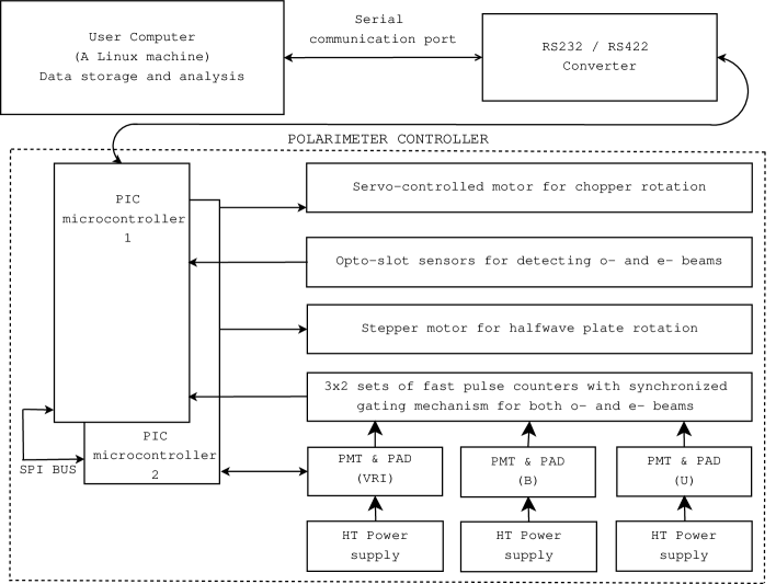
Figure 15: Schematic block diagram of the control and counting electronics.

6.1 Chopper and halfwave plate rotations

The chopper disc used for isolating the ordinary and extra-ordinary beams is made of a light weight aluminium composite material. The data acquisition timing accuracy mainly depends on the stability of the chopper rotational frequency. We have used a servo motor with the model number Smartmotor^TM SM2315, procured from Animatics, Santa Clara, California, USA. The motor has a built-in encoder and a DSP controller, and can be configured and controlled by communicating with the DSP controller through the RS232 serial communication port provided on the motor body. The motor is capable of rotating up to 10000 revolutions per minute, maintaining the same accuracy in speed throughout. The chopper is directly attached to the servo motor shaft to avoid any possible differential motion. The opto-coupled sensors associated with the rotating chopper detect the slots corresponding to the ordinary and extra-ordinary beams and generate out of phase square wave pulses of 5 V height. The rotational speed of the chopper can be set to any value between 60 and 6000 rpm through the command from the computer accurately. When the chopper rotation command along with the required rpm as the data is received from the computer by the first PIC controller, it transfers the command data to the second PIC controller through the internal SPI bus. The second PIC controller then communicates with servo motor’s DSP controller through a sequence of commands and sets the required rpm. In order to make sure that the motor is really spinning at the set rpm before the starting of the observation, the controller measures the rpm of the motor through the opto-slot sensor waveform and gives the feedback to the first controller, and thereby, to the polarimeter operating computer.

The halfwave plate is rotated using a step motor of model number MO61-FC02, procured from Superior Electric. It has a step resolution of 0.9 degree when operated in the half-step mode and completes one full rotation in 400 half-steps. The driver for the motor is designed using the standard step motor driver ICs LM297 & LM298 pair. An arbitrary starting mark is created with an opto-coupler arrangement on the gear fixed to the shaft of the step motor. Every time when the halfwave plate starts rotating for observations for the given number of position angles, it always starts from the marker position and on completion of a full rotation, it is brought back to it. This way the proper positional accuracy of the halfwave plate is ensured.

6.2 Pulse counting system

The pulse amplifier-discriminators of Model ETL AD6 and Hamamatsu Model C9744 are used to interface the ETL 9893Q/350 and Hamamatsu R943-02 photomultiplier tubes, respectively, to the pulse counters. The PADs amplify the photon generated current pluses above the set threshold level to TTL voltage pulses for counting. The pulse pair resolution of Model AD6 is 20 ns while that of C9744 is 25 ns. The pulse counter is a 24-bit TTL logic counter designed with three numbers of 74F7592, an 8-Bit bidirectional counter with 3-state output. The maximum counting frequency of the ICs is typically 100 MHz, and the pulse pair resolution is about 10 ns. They also have parallel outputs with tri-state control, and therefore, it is easy to integrate the ICs with the bus without any additional logic. One PMT requires two of these 24-bit counters, one for the ordinary beam and the other for the extra-ordinary beam. Therefore, three sets of dual counters are required for the three PMTs used. The gating pulses for the selection of the counter for the ordinary and extra-ordinary beam pulses come from the opto-sensors associated with the chopper disc. These gate pulses are monitored by the microcontroller for the count-integration purpose. The counters can store up to 16,777,216 pulses without getting saturated. A schematic block diagram of a set of pulse counter is shown in Figure 16.

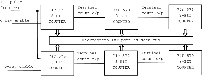
Figure 16: Schematic block diagram of a set of PMT pulse counters.

6.3 Rough estimates of maximum allowed count rates

The operating stability of a photomultiplier tube depends on the magnitude of the average anode current drawn from it. If a tube is used continuously over a long period of time at a high average anode current, variations in the output current occur even without any change in the operating conditions. A high anode current may cause even fatigue effects. It also reduces the life-time of a photomultiplier tube; the half-life, where the gain for a particular fixed high voltage drops by a factor of two, of a photomultiplier tube is proportional to the amount of total charge drawn from the anode. The charge drawn before the half-life is reached, which is on the order of 100 Coulomb, varies for individual tubes. The recommended anode current for stable performance for ETL tubes is 10 $\mu$A, while for Hamamatsu tubes it is less than 1 $\mu$A.

In the case of Hamamatsu R943-02, the anode current averaged over any interval of 30 $s$ maximum should not exceed 1 $\mu$A, otherwise permanent damage may be caused to the last dynode by the heavy electron bombardment. For ETL 9893B/350 tube the maximum specified current is 200 $\mu$A. This current can be sustained only for a brief time because ionization will eventually lead to catastrophic electrical break down in the multiplier causing permanent damage. The recommended maximum anode current for ETL tube is about 100 $\mu$A. The photomultiplier tubes should be protected from any accidental bright illumination during the observations. Peak anode currents exceeding 100 mA, but lasting only on the order of 100 ns, produced by short pulsed light sources, usually, do not cause any permanent damage to the photomultiplier tubes. Since the tubes are operated in the pulse counting mode the maximum permissible counting rates should be known so that either the electronic shutter can be closed, or the high voltage supply to the tubes can be turned down immediately in the case of any accidental illumination of the photocathode by bright sources.

If $G$ is the photomultiplier current gain, the charge contained in a pulse is given by

$$Q=1.6\times 10^{-19}\,G,$$

which produces a current

$$I_{a}=\frac{Q}{\tau}=\frac{1.6\times 10^{-19}\,G}{\tau}.$$

In the above expression $\tau$ is the full width at half maximum (FWHM) of the current pulse reaching the anode. The charge and current are expressed in Coulomb and Ampere, respectively.

Table 5: Rough estimates of the maximum allowed pulse count rates for the safe operation of the photomultiplier tubes at different operating voltages.

ETL 9893/350			H R943-02R
$I_{a}$ (max) = 100 $\mu$A			$I_{a}$ (max) = 0.5 $\mu$A
		Maximum			Maximum
Voltage (V)	Gain	counts s-1	Voltage (V)	Gain	counts s-1
1600	3$\times 10^{6}$	2.1$\times 10^{8}$	1500	5$\times 10^{5}$	6.2$\times 10^{6}$
1800	10$\times 10^{6}$	6.3$\times 10^{7}$	1700	1.6$\times 10^{6}$	2.0$\times 10^{6}$
2000	36$\times 10^{6}$	1.7$\times 10^{7}$	1900	4$\times 10^{6}$	7.8$\times 10^{5}$
2200	60$\times 10^{6}$	1.0$\times 10^{7}$	2100	9$\times 10^{6}$	3.5$\times 10^{5}$
2300	110$\times 10^{6}$	5.6$\times 10^{6}$

The number of counts registered per second by the photon counting system when the average anode current is $I_{a}$ is given by

$$n_{counts}\approx\frac{I_{a}}{1.6\times 10^{-19}\,G}\,.$$

The anode current depends on the current gain of photomultiplier, and hence, on the operating voltage. The maximum allowed count rates for different operating voltages given in Table 5 are calculated after setting $I_{a}$ to the values of the maximum allowed anode current for the safe operation of the photomultiplier tubes. The tubes should not be illuminated for an appreciable time by light sources that would produce count rates above that given in the table at the corresponding operating voltages. There will be a small contribution to the anode current from the leakage currents flowing into the anode because of the applied biasing voltages of the dynodes. The contribution to the anode current from the current pulses below the threshold level of the pulse amplifier-discriminator is neglected in the rough estimation of the allowed maximum count rates.

7 Data acquisition and analysis program

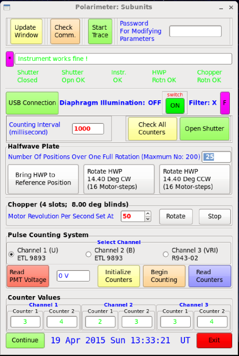
Figure 17: GUI for the instrument set-up and check-up of subunits.

A fully automated data acquisition procedure is not feasible at all; several objects will have to be observed during a night; switching between the object and background sky integration will have to be done a few unspecified number of times if the background brightness varies during the observation of an object; observations will have to be discontinued if the prevailing sky conditions become bad; spectral bands of observation will have to be changed. There are several more tasks that may have to be performed, requiring keyboard operations or mouse button clicks under very low ambient illumination, if not total darkness, that is possible when observations are in progress. Definitely, the whole procedure of data acquisition will have to be done interactively; it is extremely difficult to define in advance the sequence of observations that has to be followed.

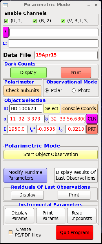
Figure 18: GUI for the beginning of observations with the polarimeter, in the polarimetric mode.

For an efficient use of the telescope time, it is highly imperative that the number of keyboard operations or mouse button clicks that is necessary to operate the instrument is kept to a minimum during observations, and thereby, avoiding any waste of time because of searching for keys or making corrections for the wrong keys entered. The acquisition program at the same time should have the provisions to interactively change the sequence of execution of its various sub-functions, executing additional functions, like, displaying intermediate values which are usually suppressed, should there be a need.

Most of the tasks in the data acquisition and reduction program that we have developed are performed with a single key-stroke or mouse-click to avoid any waste of time; only those tasks which cannot be easily undone or may cause loss of data already acquired are performed after getting confirmation. The program has the provision to store and process, including the correction for instrumental polarization, the data simultaneously in eight spectral bands. The system time required for the data reduction is negligibly small when compared to the observation time. The final results, linear polarization, position angle of polarization and the magnitude of the object, can be displayed almost immediately as soon as a full rotation of the half-wave plate is complete. If the instrumental polarization and the zero offset of the position angle are known appropriate corrections can also be made, and the final results which do not require any further processing can be obtained as soon as the object integrations are over.

The Graphical User Interfaces, which are created using GIMP Tool Kit routines, are self explanatory. There are seven main GUI’s: (1) for checking the subunits of the polarimeter and displaying its operational status, (2) for operating the instrument in the polarimetric mode, (3) for operating the instrument in the photometric mode, (4) for object observation in the polarimetric mode, (5) for sky observation in the polarimetric mode, (6) for modification of the run-time parameters and (7) for offline polarimetric data reduction; they are shown Figures 17, 18, 19, 20, 21, 22 and 23.

Table 6: Instrumental constants and runtime parameters.

Parameter	Default value
Dead-time coefficients of the three channels	0.00
Instrumental $q$ (%) and $u$ (%) and their errors in all the bands	0.00
Zero offsets in position angle (degree) in all bands	0.00
Average gain-ratios ($\alpha$) of the two beams in all bands	1.00
Standard deviations of average $\alpha$’s in all bands	0.05
Zero offsets of magnitude in all bands	0.00
Polarization efficiency in all bands	1.00

We describe briefly the interactively run data acquisition and reduction programme in the following subsections. For further details see the manual page of the program.

7.1 Tasks performed at the startup

As soon the program is initiated the polarimeter initial set-up and check-up procedure is run, reporting the status of the various sub-units. The following tasks are executed at the start-up after making sure that the communication link with the interface is functioning properly.

1. Proper rotation of the motors that control the chopper and the half-wave plate are checked.

2. The functioning of the electronic shutter is checked.

3. Outputs from the photomultipliers are checked by counting for a specified time interval.

4. The chopper is rotated at the pre-set frequency.

5. System date and time at the start-up are displayed.

If any fault is reported in the functioning of the subunits the program can be either terminated or it can be continued after rectifying the fault reported.

The time of observation is important when polarimetry of variable stars are made. If the prevailing sky conditions are good, the magnitudes computed from the data can be utilized for the photometry of the object, and for the purpose of computing the airmass of the observed object, the correct time of observation is needed. If the displayed time is wrong the system time should be properly set.

The instrumental parameters listed in Table 6 are read from a file, if such a file exists. While reading the file, if an error is encountered the program execution is terminated after giving a suitable message. If the parameter file does not exist in the specified directory, the default values given in the table are assumed for the program execution. The instrumental Stokes parameters $q$ and $u$ and their errors are in percentage and they should be listed for all the spectral bands used in the observations.

Table 7: Program runtime parameters initialized at the startup.

Parameter	Value
Chopper rotational frequency	50 Hz
Number of positions of HWP over one full rotation	25
Counting time to check the pulse counters	1000 $ms$
Object integration time	1000 $ms$
Dark counts integration time	1000 $ms$
Maximum number of dark count values plotted at a time	300
Data back-up frequency during observation	0 $s$
Output file without extension	DDMmmYY
Backup drive/directory	None
Data rejection level	5 $\sigma$
Extra-light inclusion level	5 $\sigma$

In addition to the above, the parameters listed in Table 7 are initialized with the values given against them. All these values can be altered interactively, if there is any need. The parameters used in the data acquisition, the instrumental constants used in the data reduction, and the system date and time are displayed on the terminal, indicating that the instrument is ready for carrying out observations.

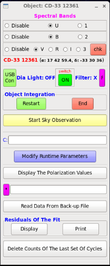
Figure 19: GUI for the object observations in the polarimetric mode.

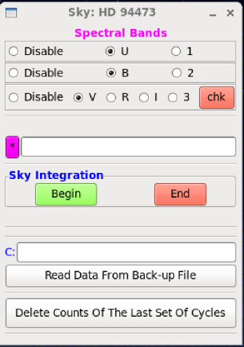
Figure 20: GUI for the sky observations in the polarimetric mode.

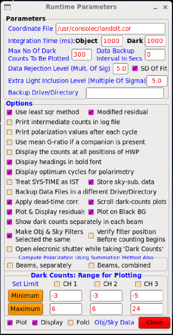
Figure 21: GUI for the modifications of runtime parameters.

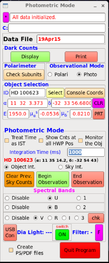
Figure 22: GUI for the polarimeter in the photometric mode.

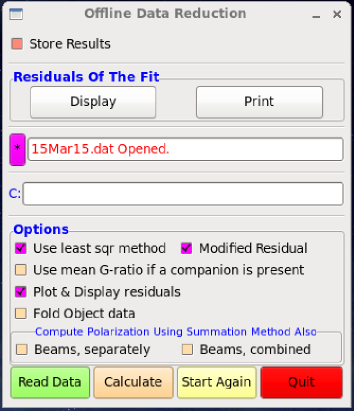
Figure 23: GUI for the offline reduction of the polarimetric data.

Several check-buttons that can be set active (On) or inactive (Off) interactively have also been provided; these are listed in Table 8. The initial settings of these toggling options, which can be either $`$On’ or $`$Off’, at the startup are indicated in the table against each of them. On setting some of the toggling option $`$On’ those particular options are executed while setting them $`$Off’ the execution of those options are suppressed. The other toggling options when set $`$On’ or $`$Off’, alternately activates one of the two different available options; these are listed in Table 9. The first option is executed if the corresponding check button is set $`$On’ and the second option, if it is set $`$Off’.

Table 8: Toggling options initialized at the startup.

Toggle option	Status
Use least square method to solve the unknowns	On
Minimize the sum of the squares of the modified residuals	On
Use standard deviation of fit to remove erroneous data	On
Print intermediate counts in the log file	Off
Print polarization values after each cycle	Off
Use average gain-ratio if a companion is present	Off
Display the counts at all half-wave plate positions	Off
Display headings in bold font	On
Display optimum cycles for polarimetry	On
Treat system time as Indian Standard Time	Off
Backup data on a USB drive after observations of each object	Off
Store sky-subtracted data for reduction later	On
Apply dead-time correction to the observed counts	On
Scroll the dark counts window (Max 300 values)	On
Plot and display the residuals of the computation	On
Plot on black background	On
Show/plot dark counts separately in each beam	On
Make object filter bands the same as those selected for sky	On
Verify filter position before counting begins	On
Compute polarization using summation method (beams, separately)	Off
Compute polarization using summation method (beams, combined)	Off
Fold object/sky data while plotting	Off
Use the given maximum/minimum limits for plotting dark counts	Off
Plot object/sky data at each position of the HWP	On
Display object/sky data at each position of the HWP	On

Table 9: Options selected when the check buttons are On and Off.

Check button active	Check button inactive
Use least square to solve the unknowns	Use elimination method to solve
Minimize the sum of the squares of the modified residuals	Minimize the sum of the squares of residuals of intensity ratios
Use standard deviation of fit to reject erroneous data	Use the expected values at each channel to reject erroneous data
Use $\alpha_{ave}$ if extra-light is present	Neglect the extra-light
Display counts at all HWP positions	Display counts only at the last position
Display headings in bold Font	Display headings in normal font to reduce the terminal brightness
Display optimum times for polarimetry	Display those for photometry
Treat system time as IST	Treat system time as UT
Scroll dark counts window	Fold and overplot with a different colour once the maximum number of specified counts are reached
Plot and display the residuals of the computation	Plot and display the raw data
Plot on black background	Plot on white background
Show/plot dark counts separately in each beam	Add the dark counts in the two beams and then display/plot
Make object filter bands the same as those selected for the sky	Make sky filter bands the same as those selected for the object
Fold object/sky data over 360 degrees while plotting	Plot the data sequentially, channel-wise
Use the given maximum/minimum limits for plotting dark counts	Choose automatically from the values available already

The dark currents of the photomultiplier tubes can be monitored when the instrument is in the Polarimetric or Photometric mode. The counts are simultaneously displayed and plotted. The terminal size (25$\times$80) set allows the display of a maximum of around 50 values in each channel at a time; however, a maximum of 300 values can be plotted at a time.

7.2 Tasks performed during object integration

As soon as the observational procedure is initiated four output files are created in the append mode: (i) a log-file, for writing a summary of the various tasks performed and some of the important information that may be needed later while analyzing the data, (ii) a file to write the polarization and position angle of the objects observed, (iii) a file to write the observed normalized Stokes parameters Q(%) and U(%), and (iv) a file to write the sky-subtracted counts, which can be processed later, if needed. During the object integration the minimum tasks that should be carried out are listed in Table 10.

Table 10: Minimum tasks to be performed during the object integration.

Tasks to be performed
Input the name of the object
Select filter-bands for observation
Begin object integration
Temporarily halt for centring of the object in the diaphragm, etc.
Terminate integration in a band, if necessary
Perform background sky integration
End the object integration to observe another object

Table 11: Minimum tasks to be performed during the background sky integration.

Tasks to be performed
Select filter-bands for observation
Begin background sky integration
Temporarily halt integration for changing the filters, if needed
Terminate integration in a band, if necessary
End background sky integration to begin or continue the object integration

The name of the object is essential to identify the polarization measurements later because the results for all the objects are stored in the same files. The name of the object, as soon as it is entered, is compared against the names of unpolarized and polarized objects contained in two separate lists to ascertain whether it is one of them. If the object is found to be in one of the lists, the appropriate designation, Z for unpolarized and P for polarized, is appended to the object name. This information can be used later while sorting the objects from the files created.

The background sky observation can be performed before or after the object integration or in between if the brightness of the background sky is suspected to be variable. It is better if the sky observations are done first so that the polarization values displayed will be the final values. If the sky is bright it is advisable to observe the sky before and after the observation of the star. The minimum tasks to be performed during background sky observation, which are similar to those performed during the object integration, are listed in Table 11.

A complete set of observations may take several tens of minutes if the object being observed is faint. Therefore, it is necessary to know the status of the observation at any instant of time. All the relevant details are displayed on the monitor so that the observer will have a clear cut understanding of what is going on, how long the process would take and what has to be done next.

The displays during both the sky and object integrations are updated after each cycle of the half-wave plate rotation so that the build-up of respective counts can be easily monitored and the integration terminated when sufficient counts are accumulated. Once the observation is stopped, either to centre the object or to discontinue the integration, along with the results of polarization measurements, the plots of the residuals of the fit are also displayed. Once the observation is ended the final results are written in the respective files.

7.3 Output files

From the mean time of observation in each spectral band, determined from the beginning and end of object integrations, the Julian day of observation is computed and recorded along with the results of polarimetry. In variable star polarimetry a continuously running time is needed; since the conversion of the civil time to Julian day is made immediately it saves the trouble of doing so later. Brief descriptions of the four output files which are created are given below.

7.3.1 File containing the log of observations

The log file contains a record of the various tasks performed during the observations. Since all the required information connected with the observations are automatically recorded or can be entered in the log-file at any time during the observation, there is no necessity of noting down anything in a register manually. This procedure, in addition to avoiding a rather cumbersome job to be performed in the ambient dim light, which is generally the case, also reduces any waste of observational time. All the instrumental constants used for the data acquisition and data reduction during the particular observing run, the beginning and end of the integrations, the number of rotations of the half-wave plate during the integration, etc. are also recorded in the log-file. Any changes made in the reduction procedure or any parameter connected with the data acquisition or reduction procedure by toggling the options are also recorded along with the times at which these changes are made. The background sky brightness used in the data reduction, and the results of the polarimetric observations are also recorded.

Intrinsic polarization in many late-type stars has been found to be closely tied-up with their light variation (Serkowski 1970a; Shawl 1975; Raveendran 1999b). A knowledge of the photometric behaviour at the time of polarimetric observations is essential for a meaningful interpretation of the polarimetric data of variable stars. If the sky transparency changes during the integration as a result of thin passing clouds, the magnitudes derived in various spectral bands will not be accurate. Since the extinction by clouds is nearly independent of wavelength in the $UBVRI$ passbands (Serkowski 1970b), the effect of transparency variations would be negligible in the colours if they are derived from simultaneous multiband observations. These colours could be effectively used in determining the photometric phases of the variable stars in the absence of accurate magnitudes. For this purpose the star-$plus$-sky counts in simultaneously observed bands are written in the log file, and if the sky observations are already available the counts due to the star are calculated and converted into magnitudes. These magnitudes should be corrected by adding $-2.5\log\{2/(1+\alpha)\}$ if the ratio of efficiencies of the two channels ($\alpha$) is significantly different from unity. In those cases where a faint component is present in one of the beams the magnitudes should be re-calculated from the listed counts. The colours of the object could be determined from these data if there is a need. Such a procedure ensures that no information available in the data collected is lost.

7.3.2 File containing polarization and position angle

This file contains the polarization (%) and position angle (degree) of the observed objects. If the instrumental polarization, polarization efficiency and position angle offset are available appropriate corrections are made before writing to these values. The errors in polarization and position angle contain the errors in the determination of instrumental polarization also. The mean Julian day of observation and the magnitude, including the gain-ratio, are also written in the file.

7.3.3 File containing normalized Q(%) and U(%)

The observed Q(%) and U(%), without any correction, including even the polarization efficiency, are written in a file; these values are stored with the idea of using a different set of corrections to the instrumental polarization and polarization efficiency at a later date, if there is a necessity of doing so when improved values of corrections available. The mean Julian day of observation, the airmass of observation and the magnitude, including the gain-ratio, are also written in the file.

7.3.4 File containing the acquired data

The sky-subtracted counts are written in this file. All the relevant information which are needed for processing the acquired data later are also written in the file along with the counts. With the data stored, the polarization values may be derived using an algorithm different from that used at the time of observation, if the situation demands.

7.4 Options available additionally

It is convenient to store the results, sometimes, in different files, for example while objects under different observational programmes or for different observers are observed in a night. For this purpose the provision to change the name of the output files interactively is also made available.

Several additional tasks can be performed to either save the data already acquired, or prevent it from being corrupted by improper data. After every predefined time interval, which can be interactively altered, all the data present in the computer memory are stored in a backup file. If there is any interruption in the data acquisition as a result of power failure or any other reason, the raw data backup file can be read and the observational procedure can be re-started from that stage onwards. It may so happen that after a re-centring of the images the object integration is re-started with the diaphragm illumination kept on. If the counts acquired then is co-added to that already existing in the memory the final data would be corrupted. If such a situation arises the ongoing integration can be discontinued and the counts co-added during the intervening period can be deleted.

Provisions are also made in the program to write the dark counts in the log-file, if required. If we want to visually inspect the residuals in the data after solving the unknown or print in the log-file that also can be done. The data points that are excluded from the solution because of large deviations are indicated against the corresponding position of the half-wave plate. Instead of the residuals the data can be displayed and plotted with an approximate fit by toggling the corresponding option. Since a full rotation of the halfwave plate produces four cycles of a sine wave, a provision to fold the data and plot it as a single sine wave cycle is also made available. It is also possible to disengage any desired channel and carry out observations in one or two spectral bands. Any relevant remarks that would be helpful in assessing the quality of the data later can also be written in the log-file at anytime; along with the remarks so entered the time of its entry is also recorded in the file. If there is a need, the dark counts can be monitored visually any time.

After the end of the integration of each object, backup of all the result files are taken on a USB drive automatically if the corresponding check button in the GUI is set active and the USB drive specified. If any problem is encountered in taking the backup a message is displayed to that effect.

8 Observational validation

The two main parameters of a polarimeter that determine its suitability for observations are the polarization it produces for an unpolarized beam and its ability to measure correctly the degree of polarization of a polarized beam without causing any depolarization. The first parameter is referred to as the instrumental polarization, and is usually determined by observing unpolarized stars with the instrument. The second parameter is the polarization efficiency, which is the numerical value obtained by the instrument for an input beam that is 100% polarized. The required beam is produced by inserting the Glan-Taylor prism in the telescope beam when an unpolarized star is observed. Ideally, the telescope-instrument combination should produce zero polarization and the instrument should have a 100% polarization efficiency. The observed data can be corrected properly for these two parameters, only if, they deviate slightly from their ideal values. In order to check whether these two parameters are determined accurately, a few polarization standards are also normally observed.

8.1 Observational procedure

The photomultiplier pulses corresponding to the intensities of the two emergent beams from the beam-displacement prism are counted separately over a full rotation of the halfwave plate at the specified equal angular intervals, starting from a reference position. The actual counting time interval for each beam over a rotational cycle of the chopper depends on its frequency of rotation since the latching pulses for the electronic pulse counters are derived from the positional sensors of the chopper. When the integrated counting time over several rotational cycles of the chopper equals to what is specified, the counting is stopped, and the resulting counts are stored. The halfwave plate is then moved to its next position, and the process is repeated at all the required positions. The entire procedure is counted as one cycle. The cycle can be repeated till the required accuracy in the measurement is achieved. After each cycle, the counts are added to the previously stored counts at the respective position of the halfwave plate. Before a new cycle begins the halfwave plate is always brought to its reference position. In order to give equal weightage to the observations in the data reduction, the number of counts accumulated at all positions of the half-wave plate should be of the same order. This requires that under poor sky conditions the observations should be repeated over several cycles of rotation of the half-wave plate, with a smaller integration time at each position of the halfwave plate. Usually, the observations in $U$ and $B$ bands will last longer than those in $V$, $R$ and $I$ bands. The integrations in $U$ and $B$ can be continued till integrations in the other bands are completed successively.

The procedure is the same for the object and the sky background that has to removed from the object $plus$ sky background counts before the data reduction. As shown in the section on optimum background sky observation, the time to be spent on sky integration is usually a small fraction of the time spent on the object integration. The optimum number of sky cycles for an observed number of object cycles and the optimum number of object cycles for an observed number of sky cycles, which are computed from the relative brightnesses of the object and sky, are displayed on the monitor.

After each cycle, the linear polarization, position angle, gain-ratio and their probable errors are displayed on the monitor. If the sky background is observed first, the displayed values will represent the actual values, otherwise, they will only be approximations. Once the integration of the object is terminated, the final values of the Stokes parameters Q(%) and U(%), the polarization (P%), the position angle ($\theta$^∘) and the mean Julian day of observation are stored in appropriate files.

8.2 Observations

The polarimeter was mounted onto the 1-m Carl Zeiss telescope at Vainu Bappu Observatory, Kavalur, and observations of several polarized and unpolarized stars were made during 14 April–30 May 2014, to determine its suitability for efficient astronomical observations. The latter group of stars were observed with and without the Glan-Taylor prism in the light path. Due to the prevalent poor sky conditions, the instrument could be used effectively only on a few nights during this period. An analysis of the observational data indicated a very high degree of mechanical stability for the instrument. We found the instrumental polarization to be very small ($<$ 0.05%). However, the polarization efficiency of the instrument was found to be 94.72%, against a normally expected value of 98-99%. It may be noted that this value is not abnormally low when we consider the fact that a measured value of 97% has been reported by Prescott et al. (2011) for the polarimeter they used.

In the data reduction program four schemes of determination of the polarization are included: (i) least square method where the sum of the squares of residuals of intensity ratio is made a minimum (equation 35), (ii) least square method where the sum of the squares of the modified residuals is made a minimum (equation 39), (iii) elimination method and (iv) summation method. The last two schemes are restricted in their use: the elimination method requires that the data are sampled at 22.5 degrees of the rotation of the halfwave plate, where a full rotation is completed in 16 steps, and the summation method will be useful if all the data samples are free from any large deviations. The four reduction schemes were applied to the observations of the unpolarized star HD 100623 through the Glan-Taylor prism obtained on 27 Apr 2014. We found that the polarizations and the position angles agreed well with each other when the two beams were used simultaneously irrespective of the reduction scheme used. However, there were differences in the probable errors derived; the first scheme gave the largest probable errors and the elimination method, the smallest errors. The smaller errors in the case of the latter method is probably because the gain-ratios are solved separately. The larger errors in the case of the first scheme is because the ratios involved when a fully polarized beam is analyzed show a very large range. All the four methods gave nearly identical results for the observations without the Glan-Taylor prism since the polarization involved was comparatively very low. As expected, the polarization derived using the beams separately showed a large difference. However, the average of the polarizations obtained separately agreed well with those derived using the other schemes.

During the April–May 2014 observing run we had used a chopper disc without blackening since the original one had gone bad. We also found that the positional sensors of the chopper were producing a few thousand counts in the $R$ and $I$ spectral bands. We blackened the chopper and modified the light-shields of the sensors apart from making slight modifications in the mounting unit of the chopper for still better stability. Observations were carried out again during February–April 2015 with the polarimeter attached to the 1-m telescope. In the following subsections we present an analysis of these observations and the results obtained.

Observations during April–May 2014 were made with different settings of the chopper speed, number of positions of the halfwave plate over a full rotation, integration times and diaphragm sizes, in order to look for any dependency on their values. Since we could not find any obvious differences in the results of the measurements, the observations during February–April 2015 were done with a chopper frequency of 50 Hz, 25 positions of halfwave plate over a full rotation, integration time of 1-s, and diaphragms of 20 $arcsec$ diameter. In addition to the $UBVRI$ bands, another broad spectral band which included both the $R$ and $I$ bands was also used for the observations. We refer to this band, which has a mean wavelength of 712 nm, in this report as $R^{\prime}$.

Figure 24: Spectral response of the neutral density filter used for the determination of the dead-time coefficient of the counting electronics associated with the $VRI$ channel.

8.3 Determination of dead-time coefficient

Equation 32 shows that the true count rates should be known to derive the dead-time coefficient ($\rho$) of the counting electronics from the observed count rates. The true count rate is actually computed by observing the same object through a neutral density filter of known attenuation coefficient ($\alpha$), which is the ratio of the incident light flux to the transmitted light flux. The counts observed through the filter should be free from any dead-time effects, which requires that $\alpha$ should be around 25–30. For this purpose, we made a suitable neutral density filter by trial and error using a photographic film. The spectral characteristic of the filter which we used is given in Figure 24.

Figure 25: Plots of the count rates at different positions of the rotating halfwave plate observed without the neutral density filter against the corresponding count rates observed with the filter. The dashed lines represent the case of zero dead-time effects for the two orthogonally polarized beams. The solid lines show the least square fit with the dead-time effect.

Figure 26: Plots of the observed count rates without the neutral density at different positions of the rotating halfwave plate against the corresponding true count rates computed from the count rates observed with the filter. The true count rates were computed using the already computed attenuation coefficients for the two orthogonally polarized beams. The dashed line represents the case of zero dead-time effects, and the solid line shows the least square fit with the dead-time effect.

A large range of count rates, which is needed for determining both the attenuation coefficient and the dead-time coefficient, can be easily obtained by observing a suitably bright star through the Glan-Taylor prism at different positions of the rotating halfwave plate. We observed HR 3482 (G5 III) and HR 4910 (M3 III) on two different nights through the Glan-Taylor prism to determine the dead-time coefficient of the counting electronics associated with the $VRI$ channel. The observational sequence was: without the filter (1 cycle), with the filter (30 cycles), without the filter (1 cycle), without the filter (1 cycle), with the filter (30 cycles) and without the filter (1 cycle) for the first object, and without the filter (2 cycles), with the filter (31 cycles) and without the filter (1 cycle) for the second object. In Figure 25 we have plotted the count rates at different positions of the rotating halfwave plate observed without the neutral density filter against the corresponding count rates with the filter observed immediately before or after. It is clear from the figure that the attenuations of the filter for the two orthogonally polarized beams are significantly different. Even though the two stars have very different spectral types, the attenuation coefficients seem to be be nearly the same for both the stars, indicating that the variation in the transmittance with wavelength seen in Figure 24 has little effect in the $V$ band for the observed objects.

Figure 27: Observed instrumental polarization in $UBVRR^{\prime}I$ bands plotted in the (Q,U) plane. The thick symbols and lines in the plots indicate the averages for the respective filter bands.

Equation 32 can be written as

$$C_{obs}=C_{true}\,e^{-\rho\,C_{true}},$$

where $C_{obs}$ and $C_{true}$ represent the observed and true count rates. If we denote the count rates with and without the neutral density as $C^{nd}$ and $C$, with $\alpha_{1}$ and $\alpha_{2}$ as the attenuation coefficients of the neutral density filter for the two orthogonal beams, the above equation can be written as

$$C_{1}=\alpha_{1}C_{1}^{nd}e^{-\rho\alpha_{1}C_{1}^{nd}}\quad\mbox{and}\quad C_{2}=\alpha_{2}C_{2}^{nd}e^{-\rho\alpha_{2}C_{2}^{nd}},$$

for the two beams. The above equations were solved simultaneously using the observed data by the method of non-linear least-squares, yielding $\alpha_{1}=$29.771$\pm$0.077, $\alpha_{2}=$ 31.457$\pm$0.080 and $\rho=$ 2.51$\pm$0.41 $\times 10^{-8}$ s. In Figure 25 the solid and dashed lines show the solutions with and without the dead-time effects for the two polarized beams. We have plotted in Figure 26 the observed counts rates against the true counts computed using the above values for the attenuation coefficients. The solid and dashed lines again show the solutions with and without the dead-time effects. The dead-time coefficient $\rho=$ 2.51$\times 10^{-8}$ s derived for the counting electronics of the $VRI$ channel is essentially the pulse pair resolution of 25 ns quoted for the pulse amplifier-discriminator C9744 used in that channel; the counters are able to handle much higher counting rates without causing any dead-time effects.

We could not determine the dead-time coefficients for the counting electronics associated with the other two channels because of the non-availability of a suitable star under clear sky conditions during the observing runs. The pulse pair resolution of pulse amplifier-discriminators AD6 used in the $U$ and $B$ channels is 20 ns, and hence, the dead-time coefficient is expected to be smaller than that of the $VRI$ channel, given above.

Table 12: Instrumental polarization in the instrument’s coordinate system. The reading on the Position Angle Device of the telescope was kept at 300 degrees.

					Number of
Band	Q (%)	U (%)	P (%)	$\theta$ (∘)	Observations
$U$	$-$0.075$\pm$0.017	0.064$\pm$0.016	0.098$\pm$0.017	69.78$\pm$4.76	29
$B$	$-$0.061$\pm$0.011	$-$0.009$\pm$0.009	0.061$\pm$0.011	93.99$\pm$4.02	41
$V$	$-$0.042$\pm$0.006	0.015$\pm$0.006	0.045$\pm$0.006	80.12$\pm$3.52	43
$R$	$-$0.045$\pm$0.006	0.008$\pm$0.009	0.046$\pm$0.006	84.86$\pm$5.42	10
$R^{\prime}$	$-$0.032$\pm$0.004	0.010$\pm$0.003	0.033$\pm$0.004	81.04$\pm$3.00	35
$I$	$-$0.044$\pm$0.005	$-$0.001$\pm$0.005	0.044$\pm$0.005	90.43$\pm$3.12	40

Figure 28: Plots of instrumental Q (%), U (%) and p (%) against the mean wavelength of the corresponding spectral band. The dashed lines show the averages of the corresponding quantities in the $BVRR^{\prime}I$ bands.

8.4 Instrumental polarization

We observed the unpolarized stars, HD 42807, HD 65583, HD 90508, HD 98281, HD 103095, HD 100623, HD 125184 and HD 144287, on several occasions. Figure 27 shows the results of the observations in the ($Q$, $U$) plane, where the individual values are plotted. The average values of the observed Q (%), U (%) and P (%) in the $UBVRR^{\prime}I$ bands are given in Table 12 and plotted against the mean wavelengths of the spectral bands in Figure 28. The observed values were corrected for the wavelength dependent polarization efficiency (see section 8.5). The table also gives the position angles (^∘) of the instrumental polarization in the instrument’s coordinate system, and the offset 20.^∘072 (see section 8.6.2) should be added to those angles to convert them to the equatorial coordinate system. It is clear from the table and the figure that the polarization produced by the telescope-polarimeter combination is small. The polarization is nearly constant in the $V-I$ spectral region, and apparently, it increases slightly towards the ultraviolet.

Figure 29: Plots of polarization efficiency and position angle against the mean wavelength of the spectral band. The dashed lines represent the middle of the respective maximum and minimum values, and the continuous line connects the mean value in each spectral band.

The polarization given in Table 12 is, most likely, produced by the telescope because a set of observations in $V$ band with a light source fed using an optical fibre the polarimeter gave almost zero polarization. This possibility can be checked by rotating the polarimeter using the Positional Angle Device and observing unpolarized stars.

Table 13: Wavelength dependence of polarization efficiency and position angle.

Spectral Band	Polarization (P%)	Position angle ($\theta$∘)
$U$	99.222$\pm$0.024	0.113$\pm$0.029
$B$	99.346$\pm$0.010	0.624$\pm$0.016
$V$	99.076$\pm$0.006	0.000$\pm$0.012
$R$	99.099$\pm$0.010	$-$0.154$\pm$0.016
$R^{\prime}$	99.151$\pm$0.004	$-$0.267$\pm$0.013
$I$	99.306$\pm$0.004	$-$0.293$\pm$0.015

8.5 Polarization efficiency

A total of 160 observations of several unpolarized stars were made with the Glan-Taylor prism in the light path of the telescope beam to determine the polarization efficiency of the instrument, which is the numerical value obtained by the instrument for an input beam that is 100% polarized. In the top panel of Figure 29 we have plotted the individual values of the polarization efficiencies obtained by us in $UBVRR^{\prime}I$ spectral bands against the corresponding mean wavelength. The averages of the polarization efficiencies in different spectral bands are given Table 13 along with their probable errors. The continuous line in the top panel of the figure connects these averages of polarization efficiencies. It is clear from the table and figure that the polarization efficiency has a slight wavelength dependence, with lower values in the $V-R$ spectral region. The polarization efficiency, which is halfway between the maximum and the minimum, is 99.211%, and it is indicated in the figure by the dashed line. The total amplitude of variation in the $U-I$ spectral region is only 0.271%. The wavelength dependence of polarization seen in the figure resembles closely the computed wavelength dependence of retardation produced by a superachromatic halfwave plate given in Figure 6.

The individual measurements of the position angle of the polarization produced by the Glan-Taylor prism is plotted in the bottom panel of Figure 29. The average of the position angles observed in the $V$ band was subtracted before plotting in the figure. The continuous line shown in the figure connects the averages of the position angles, which are given in Table 13. The middle value of the maximum and minimum of the position angles is 0.^∘165, and it is also shown in the figure. As in the case of the polarization efficiency, the position angle also shows a slight wavelength dependence. The wavelength dependence observed is almost an inverted and scaled-down version of the variation of the position angle of the effective optical axis theoretically computed for a super-achromatic halfwave plate shown in Figure 6, indicating that the fixed super-achromatic halfwave plate in the beam does not fully compensate for the variation in the position angle of the effective optical axis of the rotating plate because of the slight, but unavoidable errors in their fabrication. The total amplitude of variation in the position angle is only 0.^∘92, and the wavelength-dependent offset in the position angle can be incorporated in the data reduction procedure easily for an accurate determination of the position angles.

It is advisable to check the constancy of the polarization efficiency of the polarimeter by observing unpolarized stars through the Glan-Taylor prism once in a while during the observing runs.

The dead-time coefficient $\rho=$2.51$\times 10^{-8}$ s was incorporated in the online reduction procedure on 14 March 2015. The calculations before this date were made with $\rho=$ 0.0 s. The simple equation 31 to correct the observed polarization for the dead-time effect is valid only at low polarization values because it was derived on the assumption that the count rates are similar at the maximum and minimum of the light modulation. When the polarization efficiency of the instrument is determined using the Glan-Taylor prism, the counts registered at the lower regions of the modulation-curve will not be affected by the dead-time effects. From equation 29 we find that the change in polarization efficiency $\delta\eta_{P}$ due to a change $\delta N_{max}$ in $N_{max}$, the counts at the maximum of the modulation, is given by

$$\delta\eta_{P}=\frac{2N_{max}\eta\prime}{N_{max}(1+\eta\prime)^{2}}\,\delta N_{max}\,,$$

where $\eta\prime=(1-\eta_{P})/(1+\eta_{P})$. Making use of equation 30, the expression for $\delta\eta_{P}$ can be written as

$$\delta\eta_{P}=\frac{2\eta\prime\rho C}{(1+\rho C)^{2}}\,,$$

where $C$ is the observed count rate, taken as an approximation to the true count rate. The observed polarization efficiency will be affected by dead-time effects at large count rates only if the efficiency is very different from unity.

Figure 30: Plot of the polarization efficiency against the corresponding observed brightness.

The polarization efficiencies observed by us in $UBVRR^{\prime}I$ bands are plotted against the corresponding brightness, expressed in the magnitude scale in Figure 30. The observations plotted in the figure span a large range in brightness and from the figure we find no perceptible dependence of polarization efficiency on the brightness of the observed object in any spectral band. The count rates at the highest observed magnitude of 3.1 for the $V$ band observations plotted in the figure is 7.1$\times 10^{5}$ and the error in the polarization efficiency due to the dead-time effect, according to the above equation, would be only 0.014%, which is negligibly small when compared to the errors of individual measurements in the $V$ band. Therefore, the values for the polarization efficiencies derived by us in all the spectral bands from the data obtained before 14 March 2015 are free from any dead-time effects.

Figure 31: Plot of observed polarization against that available in the literature. The observed polarization was corrected for the wavelength-dependent polarization efficiency and the instrumental polarization. The straight line indicates an efficiency of 100 per cent for the polarimeter. The number inside the brackets indicates the number of observations obtained in the corresponding spectral band.

8.6 Observations of polarized stars

During the observing runs we observed the polarized stars, HD 21291, HD 23512, HD 43384, HD 147084, HD 154445, HD 160529, HD 183143, HD 58439, HD 77581, HD 94473, HD 127769 and HD 142863 in $UBVRR^{\prime}I$ bands. Most of the above objects were observed several times during the observing runs. The first 7 objects are considered to be standard polarized stars, and are normally used to determine the offset in the measured position angles from the standard equatorial coordinate system. Hsu & Breger (1982) have reported polarizations and position angles for these objects in $UBVR$ bands and in a band centred around 0.75 $\mu$. For the other 5 stars, Mathewson & Ford (1970) have given polarization measurements in the $B$ spectral band. The above 5 stars were included in the present observations so as to have an extended range in the polarization and brightness for the observed polarized stars.

8.6.1 Polarization efficiency

In Figure 31 we have plotted the polarization determined by us in $UBVR$ bands against the corresponding value available in the literature. The observed polarizations were corrected for the wavelength-dependent polarization efficiency of the instrument given in Table 13 and also for the instrumental polarization given in Table 12. The dead-time corrections were applied only to the observations in $VRR^{\prime}I$. The polarization measurements made before 14 March 2015 were corrected using the equation 31, using the average count rates. In $UB$ bands the corrections for the dead-time effects are expected to be negligibly small in view of the low count rates in those bands. The pulse pair resolution of the pulse amplifier-discriminator type AD6, which is used in the $U$ and $B$ channels, is 20 ns, while the type C9744, used in the $VRI$ channel is 25 ns. Therefore, the dead-time coefficient is expected to be smaller than 2.5$\times 10^{-8}$ s, and hence, the correction even at the highest observed count rate of 38000 s^-1 for HD 147084 in the $B$ band would be less than 0.09% of the observed polarization. It is clear from Figure 31 that there is an excellent agreement between the measured polarization and the corresponding value available in the literature. A linear least square fit to the data plotted in the figure gave a value of 1.0044$\pm$0.0014 for the slope.

Figure 32: Plot of observed position angle against that available in the literature. The observed position angle was corrected for the wavelength-dependent offset. The straight line has a slope of unity. The number inside the brackets indicates the number of observations obtained in the corresponding spectral band.

8.6.2 Offset in position angles

We have plotted in Figure 32 the position angles observed by us in $UBVRR^{\prime}$ against the corresponding values available in the literature. The position angles in $R^{\prime}$ band were obtained by an interpolation of the position angles in $R$ and 0.75 $\mu$ bands given in Hsu & Breger (1982). It is clear that the agreement between the measured values and those available in the literature is very good. The observed position angles were corrected for the wavelength-dependent position angle of the effective optical axis of the rotating halfwave plate given in Table 13. The offset in the position angles, in the sense, standard $minus$ observed, determined by a least square fit to the combined data plotted in Figure 32 is 20.^∘072$\pm$0.^∘044; note that this offset is with the Position Angle Device reading 300^∘. The offset obtained using such a procedure would be better than the value determined using a single standard polarized star since the position angles of some of the standards are found to vary by more than 1^∘  (Hsu & Breger 1982). The consistency in the observed position angle throughout the observational period indicates a good mechanical stability for the polarimeter, especially, in the repeatability in the positioning of the halfwave plate during each cycle.

Table 14: $UBVRI$ magnitudes and the effective wavelengths of the observation.

	Magnitudes					Effective wavelengths (nm)
Object	$U$	$B$	$V$	$R$	$I$	$U$	$B$	$V$	$R$	$R^{\prime}$	$I$
HD 21291	4.40	4.63	4.22	3.84	3.46	365	440	561	663	726	800
HD 23512	8.72	8.44	8.09	7.79	7.49	372	441	559	647	701	799
HD 43384	6.31	6.70	6.25	5.78	5.38	363	440	561	651	708	800
HD 147084	5.99	5.40	4.57	3.69	2.93	375	442	566	675	745	804
HD 154445	5.10	5.73	5.61	5.39	5.34	362	439	558	647	700	797
HD 160529	8.17	7.87	6.66	5.50	4.51	367	443	569	665	736	806
HD 183143	8.25	8.08	6.86	5.74	4.79	366	443	568	655	735	806

8.6.3 Effective wavelengths of observation

In order to compare the results of the present polarimetry of polarized stars with those available in the literature the effective wavelengths of observation are needed because the polarization is a function of wavelength and differences in the effective wavelengths of observation could give rise to substantial differences in the polarizations observed in the same spectral band with different instruments. Since the polarization varies slowly within a spectral passband normally used, the effective wavelength is a fairly good approximation to the isophotal wavelength. As these stars are reddened at different degrees, resulting in large differences in their flux distributions, there could be substantial differences in the effective wavelengths of observation when there are significant differences in the way the spectral passbands are isolated for the observations. The measurements of Hsu & Breger (1982), which form the bulk of the data against which we have compared the present observations, were obtained with the filter-detector combinations that are completely different from what we used, and therefore, the corresponding spectral passbands also would be significantly different. They had used interference filters to separate the $BVR$ spectral bands, while we used glass filters with much broader passbands.

Figure 33: Plots of the normalized fluxes of the polarimetric standards, which are used for the calculation of the effective wavelengths of observation in $UBVRI$ bands.

We computed the effective wavelengths of observation using the $UBVRI$ magnitudes of these stars in the Johnson’s system, which are listed in Table 14, and the response curves of the filter-detector combinations given in Figure 12. The $UBVRI$ magnitudes were taken from Ducati (2002) and were converted to fluxes normalized at the $V$ band, using the mean wavelengths and fluxes for a 0.0 mag star given in Johnson (1966). The error caused by using mean wavelengths for the effective wavelengths is expected to be negligible. The effective wavelengths of observation were calculated using

$$\lambda_{eff}=\frac{\int\displaylimits_{band}\lambda^{2}f(\lambda)S(\lambda)\delta\lambda}{\int\displaylimits_{band}\lambda f(\lambda)S(\lambda)\delta\lambda}\,,$$

since the number of photons detected will be proportional to $\int\lambda f(\lambda)S(\lambda)\delta\lambda$. The interpolation of fluxes at other wavelengths and extrapolation at wavelengths shorter than $U$ band were done using a four-point Lagrange formula. The fluxes at wavelengths longward of the $I$ band were obtained by linearly extrapolating the fluxes at $R$ and $I$ bands. The normalized fluxes used for the derivation of the effective wavelengths, which are listed in Table 14, are plotted in Figure 33. The effect of atmospheric extinction was included in the calculation of the effective wavelengths. We used the mean extinction coefficients at Kavalur, which are listed in Table 19, and the airmass of observation was taken as 1.5. The extinction coefficients at other wavelengths were computed again using a four-point Lagrange interpolation formula. The variation of reflectivity of the telescope mirrors with wavelength was neglected because the effect is expected to be only marginal.

Table 15: Results of the $UBVRR^{\prime}I$ polarimetry of standard stars

Band	P (%)	$\theta$ (∘)		P (%)	$\theta$ (∘)
	HD 21291			HD 23512
$U$	3.41$\pm$0.10	115.1$\pm$0.8 (1)		—	—
$B$	3.39$\pm$0.03	116.6$\pm$0.2 (1)		2.14$\pm$0.08	29.9$\pm$1.0 (1)
$V$	3.54$\pm$0.04	118.1$\pm$0.3 (1)		2.28$\pm$0.03	29.5$\pm$0.5 (2)
$R^{\prime}$	3.20$\pm$0.02	118.2$\pm$0.2 (1)		2.11$\pm$0.03	29.4$\pm$0.5 (3)
$I$	2.81$\pm$0.03	117.1$\pm$0.3 (1)		2.06$\pm$0.04	27.4$\pm$0.5 (2)
	HD 43384			HD 147084
$U$	2.62$\pm$0.03	168.7$\pm$0.3 (19)		2.69$\pm$0.03	32.2$\pm$0.3 (11)
$B$	2.86$\pm$0.02	169.9$\pm$0.2 (25)		3.50$\pm$0.02	31.8$\pm$0.1 (17)
$V$	2.97$\pm$0.01	170.4$\pm$0.1 (22)		4.23$\pm$0.02	32.2$\pm$0.1 (11)
$R$	2.86$\pm$0.01	170.8$\pm$0.1 (18)		4.39$\pm$0.02	32.4$\pm$0.1 (6)
$R^{\prime}$	2.74$\pm$0.01	170.6$\pm$0.1 (15)		4.30$\pm$0.01	32.5$\pm$0.1 (8)
$I$	2.56$\pm$0.01	170.9$\pm$0.1 (22)		4.24$\pm$0.01	32.5$\pm$0.1 (11)
	HD 154445			HD 160529
$U$	3.01$\pm$0.02	90.2$\pm$0.2 (13)		6.33$\pm$0.05	19.4$\pm$0.2 (10)
$B$	3.51$\pm$0.02	90.0$\pm$0.2 (13)		7.08$\pm$0.05	19.7$\pm$0.2 (10)
$V$	3.75$\pm$0.01	90.1$\pm$0.1 (8)		7.28$\pm$0.02	20.3$\pm$0.1 (11)
$R$	3.65$\pm$0.01	90.0$\pm$0.1 (8)		7.02$\pm$0.01	20.9$\pm$0.1 (5)
$R^{\prime}$	3.47$\pm$0.01	90.2$\pm$0.1 (5)		6.43$\pm$0.01	20.2$\pm$0.1 (5)
$I$	3.23$\pm$0.01	89.8$\pm$0.1 (8)		6.08$\pm$0.02	20.7$\pm$0.1 (10)
	HD 183143
$U$	5.04$\pm$0.09	179.1$\pm$0.7 (4)
$B$	5.77$\pm$0.07	179.4$\pm$0.1 (4)
$V$	6.16$\pm$0.01	178.8$\pm$0.3 (2)
$R$	5.87$\pm$0.01	178.6$\pm$0.1 (4)
$I$	5.18$\pm$0.02	178.6$\pm$0.2 (2)

8.6.4 Comparison with the literature values

The averages of the polarization of HD 21291, HD 23512, HD 43384, HD 147084, HD 154445, HD 160529 and HD 183143 observed by us in $UBVRR^{\prime}I$ spectral bands are given Table 15. The numbers inside the brackets indicate the number of observations in each case. In this section we make a detailed comparison of the present multiband polarimetric data of these stars, which are considered to be polarization standards, with those of Hsu & Breger (1982) and Serkowski, Mathewson & Ford (1975).

Figure 34: Plot of the polarization of HD 21291 observed in $UBVR^{\prime}I$ bands against the inverse of the corresponding wavelength. The filled circles indicate the data given in Table 15, crosses those given in Hsu & Breger (1982) and filled triangles those given in Serkowski, Mathewson & Ford (1975). The dashed line shows the interstellar polarization curve computed using the $P_{max}$ and $\lambda_{max}$ given by the former authors, and the solid line that computed using the values derived from the present polarimetry.

Figure 35: Plot of the polarization of HD 23512 observed in $BVR^{\prime}I$ bands against the inverse of the corresponding wavelength. The filled circles indicate the data given in Table 15, crosses those given in Hsu & Breger (1982) and filled triangles those given in Serkowski, Mathewson & Ford (1975). The dashed line shows the interstellar polarization curves computed using the $P_{max}$ and $\lambda_{max}$ given by the former authors, and the solid line that computed using the values derived from the present polarimetry.

Figure 36: Plot of the polarization of HD 43384 observed in $UBVRR^{\prime}I$ bands against the inverse of the corresponding wavelength. The filled circles indicate the data given in Table 15, crosses those given in Hsu & Breger (1982) and filled triangles those given in Serkowski, Mathewson & Ford (1975). The dashed line shows the interstellar polarization curves computed using the $P_{max}$ and $\lambda_{max}$ given by the former authors, and the solid line that computed using the values derived from the present polarimetry.

The polarizations in the $UBVRR^{\prime}I$ spectral bands given in Table 15 are plotted in Figures 34$-$40 against the corresponding effective wavelengths given in Table 14. The figures also show the observations of Hsu & Breger (1982) and Serkowski, Mathewson, & Ford (1975) plotted against the respective inverses of the effective wavelengths of observation, which were computed using the empirical relations given by the authors. The average airmass of observation was taken as 1.0 while computing the effective wavelengths of the observations of Hsu & Breger (1982). The errors in the measurements are also indicated in the figures.

In Figures 34$-$40 we have also plotted the interstellar polarization curve, which is the same for all stars when normalized to $\lambda_{max}$, the wavelength of maximum polarization $P_{max}$, computed using the empirical relation,

$$P=P_{max}\exp\{-1.15\ln^{2}(\lambda_{max}/\lambda)\},$$

given in Serkowski, Mathewson, & Ford (1975). We derived the values of $P_{max}$ and $\lambda_{max}$ for all the standards which we observed from the present data using the non-linear least square method, and they are listed in Table 16 along with those given Hsu & Breger (1982). In the table we have also listed the differences in the wavelength-averaged position angles obtained by them and us.

Hsu & Breger (1982) had reported that several stars which are used as standards definitely show polarimetric variability in the order of 0.3%. We observed two of the stars, namely, HD 43384 and HD 183143, for which variabilities have been reported by them. Hsu & Breger (1982) found HD 43384 to show changes of 0.25% and 2^∘  in $P$ and $\theta$ observed in the $V$ band. A variability of 0.2–0.3% in polarization in the $V$ band has been reported by the above authors for HD 183143 also. The averages values of polarization in $UBVRI$ bands obtained by us for both these objects are in excellent agreement with those given by Hsu & Breger (1982), indicating that these objects exhibit no long-term variations. The mean values of position angles observed by us are essentially the same as those reported by the above authors, and so are the the values of $P_{max}$ and $\lambda_{max}$ .

Figure 38 shows that the present observations of HD 154445 agree well with those of Hsu & Breger (1982) and Serkowski, Mathewson & Ford (1975). The present values of $P_{max}$, $\lambda_{max}$ and the average position angle of the star are the same as those given by the former authors. The polarizations in $B$ and $V$ reported by Serkowski, Mathewson & Ford (1975) for this star are about 0.1% lower than those observed by Hsu & Breger (1982) and us.

From Figure 37 we find that in the case of HD 147084 the polarizations in the $R-I$ region observed by us are about 0.1% below those observed by Hsu & Breger (1982). The $VRR^{\prime}I$ observations of both HD 21291 and HD 147084 were done through neutral density filters of optical density 1.0. The transmission of the filter was taken into account while computing the effective wavelengths in these bands. The vendor of this filter has provided the transmission values only up to 750 nm, above which the transmission was assumed to be constant while computing the effective wavelengths. The effective wavelengths of the $R^{\prime}$ and $I$ bands could be longer than what we derived. However, the close agreement in the polarization of HD 21291 in the $R-I$ obtained by us with those obtained by Hsu & Breger (1982) rule out any large deviations. It may be noted from Figure 33 that the normalized flux of HD 147084 in the $R-I$ spectral region is much higher than that of HD 21291. The positions angles of HD 147084 in the $R-I$ spectral region are marginally higher than those obtained by the above authors. It is possible that the discrepancy in the polarization in the $R-I$ region is due to a variability of the object. The values of $\lambda_{max}$ are the same in both the cases.

Figure 39 shows that the polarizations of HD 160529 observed by us agree well with those reported by Hsu & Breger (1982). However, the values of $\lambda_{max}$ differ by about 0.012 $\mu$, which is significant when compared to the errors in their determinations. We did a least square solution of their data, which yielded $P_{max}=$7.36$\pm$0.04 and $\lambda_{max}=$ 0.534$\pm$0.004, which are almost the same as those given by the present data. It may be noted that Serkowski, Mathewson & Ford (1975) had reported a value of 0.530 $\mu$ for the $\lambda_{max}$ of this object.

The polarizations and position angles of HD 21291 and HD 23512 obtained by us also agree with those obtained by Hsu & Breger (1982), even though we have observed these objects just once or twice. In the case of HD 23512, the difference in the values of $\lambda_{max}$ obtained by us and the above authors is because we do not have the $U$ band data and the polarization obtained by us in $B$ band is slightly more than that obtained by them.

Figure 37: Plot of the polarization of HD 147084 observed in $UBVRR^{\prime}I$ bands against the inverse of the corresponding wavelength. The filled circles indicate the data given in Table 15, crosses those given in Hsu & Breger (1982) and filled triangles those given in Serkowski, Mathewson & Ford (1975). The dashed line shows the interstellar polarization curves computed using the $P_{max}$ and $\lambda_{max}$ given by the former authors, and the solid line that computed using the values derived from the present polarimetry.

Figure 38: Plot of the polarization of HD 154445 observed in $UBVRR^{\prime}I$ bands against the inverse of the corresponding wavelength. The filled circles indicate the data given in Table 15, crosses those given in Hsu & Breger (1982) and filled triangles those given in Serkowski, Mathewson & Ford (1975). The dashed line shows the interstellar polarization curves computed using the $P_{max}$ and $\lambda_{max}$ given by the former authors, and the solid line that computed using the values derived from the present polarimetry.

Table 16: $\lambda_{max}$ and $P_{max}$ of the observed polarized stars.

	Present study		Hsu & Breger 1982		$\Delta\theta_{mean}$
Object	$P_{max}$	$\lambda_{max}$	$P_{max}$	$\lambda_{max}$	(HS $-$ PS)1
HD 212912	3.54$\pm$0.03	0.525$\pm$0.008	3.53$\pm$0.02	0.521$\pm$0.003	$-$1.03$\pm$0.27
HD 23512	2.29$\pm$0.02	0.569$\pm$0.011	2.29$\pm$0.01	0.600$\pm$0.006	$+$0.89$\pm$0.41
HD 43384	3.02$\pm$0.02	0.533$\pm$0.005	3.01$\pm$0.04	0.531$\pm$0.011	$+$0.24$\pm$0.28
HD 147084	4.37$\pm$0.03	0.697$\pm$0.007	4.46$\pm$0.03	0.695$\pm$0.006	$-$0.25$\pm$0.08
HD 154445	3.73$\pm$0.01	0.556$\pm$0.002	3.73$\pm$0.01	0.558$\pm$0.002	$-$0.03$\pm$0.07
HD 183143	6.12$\pm$0.01	0.552$\pm$0.002	6.08$\pm$0.05	0.551$\pm$0.006	$-$0.35$\pm$0.11
HD 1605293	7.37$\pm$0.02	0.531$\pm$0.002	7.31$\pm$0.02	0.543$\pm$0.003	$-$0.38$\pm$0.21
(1)HS$-$Hsu & Breger (1982); PS$-$ Present Study.
(2) $U$ band polarization was not used while deriving $P_{max}$ and $\lambda_{max}$.
(3) We get $P_{max}=$ 7.36$\pm$0.04 and $\lambda_{max}=$0.534 $\pm$0.004 from the data of Hsu & Breger (1982).

Figure 39: Plot of the polarization of HD 160529 observed in $UBVRR^{\prime}I$ bands against the inverse of the corresponding wavelength. The filled circles indicate the data given in Table 15, crosses those given in Hsu & Breger (1982) and filled triangles those given in Serkowski, Mathewson & Ford (1975). The dashed line shows the interstellar polarization curves computed using the $P_{max}$ and $\lambda_{max}$ given by the former authors, and the solid line that computed using the values derived from the present polarimetry. The dotted line shows the solution obtained by us using the data of Hsu & Breger (1982).

Figure 40: Plot of the polarization of HD 183143 observed in $UBVRI$ bands against the inverse of the corresponding wavelength. The filled circles indicate the data given in Table 15, crosses those given in Hsu & Breger (1982) and filled triangles those given in Serkowski, Mathewson & Ford (1975). The dashed line shows the interstellar polarization curves computed using the $P_{max}$ and $\lambda_{max}$ given by the former authors, and the solid line that computed using the values derived from the present polarimetry.

8.7 Gain-ratios

Figure 41: Gain ratios of the two beams in $UBVRI$ bands, and the total number of observations are 241, 302, 228, 238 and 188, respectively. The average values and their standard deviations are 0.977$\pm$0.028, 1.051$\pm$0.018, 0.968$\pm$0.013, 0.966$\pm$0.013 and 0.967$\pm$0.012.

The histograms of the gain-ratios of the two beams derived from the observations are plotted in Figure 41. The gain-ratios observed in $R^{\prime}$ were combined with those observed in $R$ band in forming the histograms. The average values and their standard deviations in the $UBVRI$ spectral bands are 0.977$\pm$0.028, 1.051$\pm$0.018, 0.968$\pm$0.013, 0.966$\pm$0.013 and 0.967$\pm$0.012, respectively. It may be noted that the mean values of the gain-ratios in the $VRI$ bands are almost the same. The average values in all the spectral bands are close to unity, as they are expected to be, if the Fabry lenses are properly placed. The spread in the observed gain-ratios results mainly from the slight differences in the image centring on different occasions. Any significant deviations in the gain-ratios from the above averages may be indicative of problems with the counting electronics, or the presence of a faint component in one of the beams.

8.8 Overhead time

The error in the measured polarization due to photon noise depends on the total counts accumulated, which means that for an efficient use of the telescope time the available time should be used entirely for counting. This is not possible because the two beams are observed alternately, and the counting can be done only during the interval when the corresponding slot in the rotating chopper does not obstruct the diaphragm as seen by the photomultiplier. The slots in the chopper are separated by a blind sector of 8 degree in size during the passage of which below the diaphragm no counting can be done. Similarly, counting should begin only after the halfwave plate stops completely at each position, otherwise, there will be a certain amount of depolarization. Additionally, several delays, lasting a few milliseconds, are introduced in the program by trial and error for the effective communication between the computer and the interface.

In Figure 42 we have plotted the total time taken against the actual counting time at each position of the halfwave plate. The total time was calculated for each integration time from the time taken to complete one cycle of rotation of the halfwave plate, and the actual time during which counting was done was calculated from the chopper frequency and the sizes of the blind sectors in the chopper disc. From the figure we find that there is an overhead of about 300 ms spent at each position of the halfwave plate. The fractional time lost can be reduced by giving a higher integration time and choosing a lower number for the positions of the halfwave plate at which integrations are made during its full rotation.

Figure 42: Plot of the total time taken per halfwave plate position against the actual time over which counting is done. The straight line represents a linear least square fit to the data.

Most of the overhead time is spent while waiting for the halfwave plate to stop completely at each position. Probably, this can be reduced slightly by trial and error.

The factor of 1.10 is essentially caused by the blind sectors in the chopper, and by re-designing the chopper this factor can be reduced slightly. The latching pulses for the counters are derived from the sensors which monitor the positions of the slots in the chopper. A perfect straight line fit to the data shown in Figure 42 is a clear indication of the stability in the rotational frequency of the chopper. If there were any systematic losses in the detection of the latching pulses during the chopper rotations, the line would have shown a larger slope.

8.9 Limiting magnitudes

From the observed data, we computed the count rates expected from a 10.0 mag star in $UBVRI$ bands along with the probable errors in polarization arising from the statistical fluctuations in the total counts in 10 minutes of integration in those bands, and the results are given in Table 19. We used the highest observed count rates in each band for different stars to scale down the count rates to that of a 10.0 mag star. The average air mass of observation is also given in the table. The overhead time and the time required for background sky integration, which would be only a fraction of the above timings even if the sky is moonlit and the object brightness is comparable to the sky brightness, were not included in the computation.

Table 17: Wavelength-independent parameters used to compute the expected counts.

Parameter	Value
Telescope aperture	1 $m$
Central obscuration	0.40
Reflectivity of the telescope	0.70
Transmittance of the calcite block	0.90
Transmittance of the half-wave plate	0.95

Table 18: Wavelength dependent parameters used to compute the expected counts.

Parameter	$U$	$B$	$V$	$R$	$I$
Flux for 0 mag $F_{\lambda}$ (W $m^{-2}\,nm^{-1}\times 10^{11})$	4.35	7.20	3.92	2.26	1.23
Mean wavelength $\lambda$ ($nm$)	357	437	561	652	801
Bandwidth $\Delta\lambda$ ($nm$)	69	54	94	129	149
Filter-detector efficiency	0.22	0.16	0.12	0.09	0.09

Table 19: Scaled down count rates and the corresponding probable errors in polarization (%) for a 10.0 mag star in 10 minutes of integration, the expected photon rates, and the deficiency factors in the observed count rates ($\gamma$). Overhead time was not included in computing the probable errors.

Filter	Air	Scaled	p. e.	FWHM		Expected
band	mass	c s-1	(%)	(nm)	$k_{\lambda}$	p s-1	$\gamma$
$U$	1.03	527	0.18	69	0.75	11482	22
$B$	1.03	836	0.13	54	0.40	18461	22
$V$	1.06	2289	0.08	94	0.25	19318	8
$R$	1.08	2104	0.08	129	0.15	14623	7
$I$	1.06	1501	0.10	149	0.10	11904	8

The number of photoelectrons produced per second can be calculated using

$$n_{pe}=\frac{10^{-0.4\,m}\,\pi\,F_{\lambda}\,\Delta\lambda\,T_{atm}\,T_{total}\,q\,\lambda\,D_{eff}^{2}}{8\times 10^{6}\,h\,c},$$

where $m$ is the magnitude of the object, $F_{\lambda}$, the flux density for a 0 mag A0V star, and $h$ and $c$, the Planck constant and velocity of light, $\lambda$ and $\Delta\lambda$ the effective wavelength and bandwidth of observation, $T_{atm}$, the atmospheric transmittance, $T_{total}$, the total effective transmittance and reflectivities of the various optical elements in the light path, $q$, the quantum efficiency of the detector, and $D_{eff}$, the effective diameter of the telescope. On inserting the numerical values of the constants, the above expression reduces to

$$n_{pe}=1.975\times 10^{15}\,F_{\lambda}\,10^{-0.4\,m}\,\Delta\lambda\,T_{atm}\,T_{total}\,q\,\lambda\,D_{eff}^{2},$$

where $F_{\lambda}$ is in $W\,m^{-2}\,nm^{-1}$, $\lambda$ and $\Delta\lambda$ in $nm$, and D in $m$. The fact that only 50 per cent of the photons collected by the telescope are incident on the photocathode has been taken into account in the above expression.

Using the above expression and the parameters given Tables 17 and 18 we computed the number of counts per second expected from a 10.0 mag star, and the results are also given Table 19. The absolute fluxes for a 0 mag A0V star were taken from Johnson (1966) for the $UBV$ bands and from Bessel (1979) for the $RI$ bands. The bandwidths and the combined responses of the filter-detector combination were read from Figure 12. The table also gives the deficiency factor ($\gamma$) of observed counts, which is the ratio of the the expected photon rates to the scaled down count rates for 10.0 mag star. The FWHMs of the bands estimated from the plots shown in Figure 12, and the mean extinction at VBO usually observed during the January–March period, which were used for the computations, are also given in the table.

Figure 43: Plot of the difference in the PMT chamber- and ambient-temperatures for different settings of cooling against the time elapsed after switching on the cooling unit.

Figure 44: Plot of the temperature of the PMT chamber against the ambient temperature. The straight line represents a constant difference of 44.3^∘C with a standard deviation of 0.4^∘C.

From Table 19 we see that the deficiency factors in the $UBVRI$ bands are 22, 22, 8, 7 and 8, respectively. The reflectivity of the telescope was taken as 70% for the computation of the expected photon rates. The implied reflectivity of about 84% for the mirrors is likely to be on the higher side, considering the fact that the mirrors were aluminized a few years back. The dichroic filters used in the $U$ and $B$ channels were acquired more than 12 years back. There is also a possibility that their reflectivities and transmittances have deteriorated over time, even though they were kept inside their boxes. These factors would have increased the deficiency factors in all the spectral bands in a similar way.

The identical deficiency factors in the $U$ and $B$ are almost three times those of $VRI$ bands, which are again identical within observational uncertainties. It may be noted that both the $U$ and $B$ bands have identical photomultipliers and pulse amplifier-discriminators, and the photomultipliers were operated at the same high voltages of 2300 V. The identical photon deficiency factors for these bands indicate the definite possibility that all the detected photons were not counted. The photomultipliers at 2300 V were already operated at very high gains (see Table 5). The discriminator level is factory set in AD6 model pulse amplifier-discriminators, and they may not be actually set at the valley of the pulse height distribution of the photomultipliers used. The possibility of using a pre-amplifier in these channels should be examined. It is likely that a fraction of the deficiency factor in the $VRI$ channel also arises from not counting all the detected photons since poor reflectivities of the telescope mirrors may not be able to account for the rather high deficiency factor of 8 observed in that channel. From Table 5 we see that the Hamamatsu tube also has a very high gain when it is operated at a high voltage of 1900 V. The discriminator level of C9744 can be adjusted manually. The possibility of lowering the discriminator level in the $VRI$ channel also should be examined. If the output pulses from the amplifier-discriminators show a large range, the pulse counters may not be responding to the low amplitude pulses. In such a case introducing a high bandwidth pulse amplifier before the counters might help in reducing the deficiency factor.

8.10 Cooling characteristics of FACT50

As already mentioned, the Hamamatsu R943-02 tube is mounted in FACT50 model chamber, which is of forced air-cooled type, for reducing the dark counts. In Figure 43 we have plotted the observed cooling curves of this model for different temperature settings. Along the vertical axis in the figure we have plotted the difference in temperatures, in the sense, chamber temperature minus ambient temperature. We find from the figure that at the coolest setting, which is usually the case while observing, it takes about two hours for the chamber to attain the maximum difference in temperature with respect to the ambient, and hence, the cooling unit should be switched on at least two hours before the beginning of the observations.

In Figure 44 we have plotted the PMT chamber-temperatures observed after three hours of switching on of the cooling unit against the corresponding ambient temperature. Probably, the difference in temperature attained does not depend on the ambient temperature. The average difference in temperature observed is 44.3^∘C with a standard deviation of 0.4^∘C. The PMT temperature will be varying with the variation in the ambient temperature over the course night. However, this will not have adverse effects since the ambient temperature will not be varying significant during the period of observation of an object.

Publications

1. A new three-band, two beam astronomical photo-polarimeter, G. Srinivasulu, A. V. Raveendran, S. Muneer, M. V. Mekkaden N. Jayavel, M. R. Somashekar, K. Sagayanathan, S. Ramamoorthy, M. J. Rosario, K. Jayakumar, 2014, Bull. Astr. Soc. India, 42, 165

2. Linear Polarization Measurements of Nova Sco 2015  (PNV  J17032620-3504140), S. Muneer, G. C. Anupama, A. V. Raveendan, 2015,   The Astronomer’s Telegram, #7161

3. UBVRI Polarimetry of Nova Sgr 2015 #2, S. Muneer, G. C. Anupama, A. V. Raveendran, A. Muniyandi, R. Baskar, 2015, The Astronomer’s Telegram, #7310

References

- [1] Ashok, N. M., Chandrasekhar, T., Bhatt, H. C., & Manoj, P., 1999, IAUC 7103.
- [2] Bessel, M. S., 1979, Publs Astr. Soc. Pacific, 91, 589.
- [3] Bessel, M. S., 1993, in Stellar Photometry Current Techniques and Future Developments, IAU Coll. No. 136,
- [4] Bhatt, H. C. & Manoj, P., 2000, Astron. Astrophys., 362, 978.
- [5] Brand, P. W. J. L., 1971, Optica Acta, 18, 403. (eds: C.J.Butler, I Elliot, Cambridge University Press), p.22.
- [6] Breger, M., 1979, Astrophys. J., 233, 97.
- [7] Deshpande, M. R., Joshi, U. C., Kulshrestha, A. K., et al., 1985, Bull. Astron. Soc. India, 13, 157.
- [8] Fernie, J. D., 1976, Publs Astr. Soc. Pacific, 88, 969.
- [9] Frecker, J. E. & Serkowski, K., 1976, Appl. Optics, 15, 605.
- [10] Gordon, R. W., 1988, Sky & Telescope, 75, 490.
- [11] Harris, W. E., Fitzgerald, M. P. & Reed, B. C., 1981, Publs Astr. Soc. Pacific, 93, 507.
- [12] Henden, A. A. & Kaitchuk, R. H., 1982, Astronomical Photometry, New York, Van Nostrand: London, Heffers Book Sellers
- [13] Hiltner, W. A., 1962, in Astronomical Techniques, ed.: W.A.Hiltner, The University of Chicago Press, London, p.229.
- [14] Hough, J. H., Peacock, T. & Bailey, J. A., 1991, Mon. Not. Royal Astr. Soc., 248, 74.
- [15] Hsu, J. & Breger, M., 1982, Astrophys. J., 262, 732.
- [16] Ducati, J. R.,2002, Catalogue of stellar photometry in Jonsons’s 11-color system.
- [17] Jain, S. K. & Srinivasulu, G., 1991, Opt. Eng., 30, 1415.
- [18] Jefferys, W. H., 1980, Astron. J., 85, 177.
- [19] Johnson, H. L., 1966, Annual Rev. Astr. Astrophys., 4, 193.
- [20] Kameswara Rao, N. & Raveendran, A. V., 1993, Astron. Astrophys., 274, 330.
- [21] Kikuchi, S., 1988, Bull. Tokyo Astron. Obs., Second Series No. 281, 3267.
- [22] Kopal, Z., 1959, Close Binaries, Chapman and Hall, London
- [23] Kormendy, J., 1973, Astron. J., 78, 255.
- [24] Kron, G. E. & Gordon, K. E., 1958, J. Royal Astr. Soc. Canada, 51, 17.
- [25] Levi, 1980, in Applied Optics, A guide to optical system Design, Vol. 2, John Wiley & Sons, New York
- [26] Magalhaes, A. M., Benedetti, E. & Roland, E. H., 1984, Publs Astr. Soc. Pacific, 96, 383.
- [27] Magalhaes, A. M. & Velloso, W. F., 1988, in Polarized Radiation of Circumstellar Origin, (eds: G.V.Coyne et al., Vatican Observatory, Vatican City State), p.727.
- [28] Manoj, P., Maheswar, G. & Bhatt, H. C., 2002, Bull. Astr. Soc. India, 30, 657.
- [29] Mathewson, D. S. & Ford, V. L., 1970, Mem. Royal astr. Soc., 74, 139.
- [30] McCarthy, D. E., 1967, Appl. Optics, 6, 1896.
- [31] McDavid, D., 1999, Publs Astr. Soc. Pacific, 111, 494.
- [32] Mekkaden, M. V., 1998, Astron. Astrophys., 340, 135.
- [33] Mekkaden, M. V., 1999, Astron. Astrophys., 344, 111.
- [34] Moffett, T. J. & Barnes, T. G., 1979, Publs Astr. Soc. Pacific, 91, 180.
- [35] Murdin, P. M., 1979, Observatory, 99, 216.
- [36] Parthasarathy, M., Jain, S. K. & Bhatt, H. C., 2000, Astron. Astrophys., 355, 221.
- [37] Piirola, V., 1973, Astron. Astrophys., 27, 382.
- [38] Piirola, V., 1988, in Polarized Radiation of Circumstellar Origin, (eds: G. V. Coyne et al., Vatican Observatory, Vatican City State), p.735.
- [39] Prescott, M. K. M., Smith, P. S., Schmidt, G. D., & Dey, A., 2011, Astrophys. J Letters, 730, L25.
- [40] Ramaprakash A. N., Ranjan Gupta, Sen A. K. & Tandon S. N., 1998, Astron. Astrophys., 128, 369.
- [41] Raveendran, A. V., 1999a, Mon. Not. Royal Astr. Soc., 303, 595.
- [42] Raveendran, A. V., 1999b, Proceedings of the Second Solar Polarization Workshop: Solar Polarization, (eds: K.N.Nagendra, J.O.Stenflo, Kluwer Academic Publishers, Netherlands), p.507.
- [43] Scaltriti, F., Piirola, V., Cellino, A. et al., 1989, Mem Soc. Astron. Italy, 60, 243.
- [44] Scarborough, J. B., 1964, Numerical Mathematical Analysis, Oxford Book & Stationery Co., Calcutta.
- [45] Scarrott, S. M., 1991, Vistas in Astr., 34, 163.
- [46] Schwarz, H. E. & Piirola, V., 1999, Nordic Optical Telescope Operating Manual No. 2
- [47] Serkowski, K. & Chojnacki, W., 1969, Astron. Astrophys., 1, 442.
- [48] Serkowski, K., 1970a, Astrophys. J., 160, 1107.
- [49] Serkowski, K., 1970b, Publs Astr. Soc. Pacific, 82, 908.
- [50] Serkowski, K., 1974a, in Planets, Stars and Nebulae Studied with Photopolarimetry, (ed.: T.Gehrels, Tucson, University of Arizona Press), p.135.
- [51] Serkowski, K., 1974b, in Methods of Experimental Physics, 12 Part A, (eds: M.L.Meeks, N.P.Carleton, Academic Press, New York), p.361.
- [52] Serkowski, K., Mathewson, D. S., Ford, V. L., 1975, Astrophys. J., 196, 261.
- [53] Shawl, S. J., 1975, Astron. J., 80, 602.
- [54] Subrahmanyam, N., 1980, A Text Book of Optics, S.Chand & Company Ltd., New Delhi.
- [55] Van de Hulst, H. C., 1957, Light Scattering by Small Particles, John Wiley & Sons, New York.
- [56] Young, A. T., 1967, Astron. J., 72, 747.
- [57] Young, A. T., 1970, Appl. Optics, 9, 1874.
- [58] Young, A. T., Genet, R. M., Boyd, L. J., et al., 1991, Publs Astr. Soc. Pacif., 103, 221.