Bayesian Inference for Latent Biologic Structure with Determinantal Point Processes (DPP)

Abstract

We discuss the use of the determinantal point process (DPP) as a prior for latent structure in biomedical applications, where inference often centers on the interpretation of latent features as biologically or clinically meaningful structure. Typical examples include mixture models, when the terms of the mixture are meant to represent clinically meaningful subpopulations (of patients, genes, etc.). Another class of examples are feature allocation models. We propose the DPP prior as a repulsive prior on latent mixture components in the first example, and as prior on feature-specific parameters in the second case. We argue that the DPP is in general an attractive prior model for latent structure when biologically relevant interpretation of such structure is desired. We illustrate the advantages of DPP prior in three case studies, including inference in mixture models for magnetic resonance images (MRI) and for protein expression, and a feature allocation model for gene expression using data from The Cancer Genome Atlas. An important part of our argument are efficient and straightforward posterior simulation methods. We implement a variation of reversible jump Markov chain Monte Carlo simulation for inference under the DPP prior, using a density with respect to the unit rate Poisson process.

KEY WORDS: Biomedical; Determinantal point process; Latent structure; Repulsive; Reversible jump Markov chain Monte Carlo.

1 Introduction

Independent priors for latent structure are almost never appropriate in biomedical inference. Nevertheless, they are widely used, simply for technical convenience and the lack of good alternatives. In this paper we argue for an attractive class of such alternative models in typical inference problems in biostatistics and bioinformatics.

We discuss the use of the determinantal point process (DPP) for modeling latent biologic structure. In particular, we focus on mixture models and feature allocation problems, when the latent components are to be interpreted as biologically meaningful structure. For example, in the case of a mixture model, we might want to interpret components of a mixture as clinically meaningful patient subpopulations. Similarly, when using feature allocation to model latent tumor cell subpopulations we might want to interpret the features as substantially distinct subclones (Xu et al.,, 2015). In both cases, an important aspect of the problem is the preference for the latent elements being diverse. Such inference is poorly formalized by traditionally used independent priors. We suggest the DPP prior as an attractive alternative to implement repulsive priors. The use of the DPP for mixture models is not novel. It was originally proposed in Affandi et al., (2013), but remains curiously under-used in biomedical literature. The contribution of the following discussion is the emphasis on problems with small to moderate size mixtures, the extension to inference for general latent structure, and the detailed posterior Markov chain Monte Carlo (MCMC) scheme, including easy to implement transdimensional posterior simulation across different size latent structures.

For the moment we restrict attention to parametric mixture models, to be specific and also because such models are perhaps the most common models for latent structure in biomedical applications. For example, popular Bayesian models for clustering and inference on patient subpopulations are variations of the following model. Let $y_{i}$ denote a response for the $i$-th patient. We assume

$$y_{i}\sim\sum_{h=1}^{H}w_{h}\,p(y_{i}\mid\mu_{h}),$$ (1.1)

$i=1,\ldots,n$, including possibly $H=\infty$. The component-specific sampling model $p(y_{i}\mid\mu_{h})$ could be, for example, a survival model with parameters $\mu_{h}$, possibly including a regression on patient covariates. The use of independent priors for component-specific parameters $\mu_{h}$ then gives rise to concerns about over-fitting that generates redundant mixture components with similar parameters, leading to unnecessarily complex models and poor interpretability. In particular, such over-fit compromises the interpretation of the mixture components as biologically meaningful structure. Rousseau and Mengersen, (2011) argued that such concerns were asymptotically partially mitigated with carefully chosen priors. Alternatively, Petralia et al., (2012) proposed a class of repulsive priors for mixture components. The proposed repulsive prior was based on a distance metric in which small distances were penalized. They showed that using repulsive priors on location parameters resulted in better separated clusters, while keeping the density estimation accurate. However, posterior computations are complex and do not readily extend to high dimensional cases.

An alternative interpretation of (1.1) is as a mixture, $y_{i}\sim\int p(y_{i}\mid\mu)\,dG(\mu)$, with respect to a discrete probability measure $G=\sum w_{h}\delta_{\mu_{h}}$. If the model is completed with a Dirichlet process (DP) prior on $G$ the popular DP mixture model is obtained. See, for example, Ghoshal, (2010) for a review of such nonparametric Bayesian models. Importantly, the DP prior includes independence across $\mu_{h}$.

For later reference note that (1.1) can be equivalently written as a hierarchical model with latent indicators $s_{i}$,

$$y_{i}\mid s_{i}=k\sim p(y_{i}\mid\mu_{k})\mbox{ and }p(s_{i}=k)=w_{k}.$$ (1.2)

Interpreting the latent indicators as cluster membership indicators, model (1.2) includes inference on a random partition $\bm{s}=(s_{1},\ldots,s_{n})$ of $\{1,\ldots,n\}$. Let $S_{k}=\{i:\,s_{i}=k\}$ denote the $k$-th cluster. To avoid the notion of empty clusters, that is $|S_{k}|=0$, we re-arrange the indexing of the $\mu_{h}$ to start with $h=1,\ldots,K$ corresponding to non-empty clusters. Again, an independent prior on the cluster-specific parameters $\mu_{h}$ complicates a meaningful interpretation of posterior inference on the random partition $\bm{s}$.

In this paper we argue for an alternative model that replaces the independent prior on $\mu_{h}$ by the repulsive DPP (Macchi,, 1975). Recent reviews of the DPP appear in Lavancier et al., (2015) and, specifically for finite state spaces, in Kulesza and Taskar, (2012). The use of the DPP as a prior for statistical inference in mixture models, we believe, is first discussed in Affandi et al., (2013). The main contributions of this paper are the recognition of the DPP as an attractive prior for latent features in general latent structure models, including mixture models and latent feature allocation as specific examples; the discussion of DPP mixtures specifically when one wants to interpret latent structure as biologically meaningful features; and an easily implemented posterior simulation scheme for a moderate number of latent structures, as is typical for biomedical inference problems. Posterior simulation is implemented as a variation of reversible jump (RJ) MCMC simulation (Green,, 1995) for a density with respect to the unit rate Poisson process.

2 Motivating Example

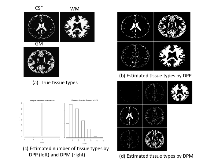
Figure 1: BrainWeb images. Panel (a) shows the three true tissue types: CSF, WM and GM. Panel (b) shows the estimated tissue types under the DPP prior. Panel (c) shows the estimated number of tissue types by DPP (left) and DPM (right). Panel (d) shows the estimated tissue types under the DPM prior.

Magnetic resonance imaging (MRI) is an effective technique for studying the human brain. For example, MRI volume estimates of white matter (WM), gray matter (GM), cerebrospinal fluid (CSF), and their spatial distribution help the diagnosis of degenerative brain illnesses, like Alzheimer’s disease (DeCarli et al.,, 1992). Therefore, accurate clustering of MRI data according to tissue types is vital to diagnosis and clinical research. To illustrate, we download a sample of simulated imaging data from BrainWeb (Cocosco et al.,, 1997) for slice number 92. Figure 1a depicts the ground truth components for CSF, WM and GM. We implement inference under model-based clustering with a DPP prior and a similar model based on the widely used Dirichlet process mixture (DPM) model. Model details will be discussed later. For the moment we only intend to highlight the nature of the inference under the two models to motivate the upcoming discussion. Figure 1c shows the posterior distribution $p(K\mid data)$ on the number of clusters estimated under the DPP prior (left panel) and the DPM prior (right panel). As shown in Figure 1b, the DPP clustering model identifies four clusters, three of which match the simulation truth and the last one is simulated noise. In contrast, inference under the DPM model finds seven clusters, only three of them having a meaningful explanation.

3 Determinantal Point Process (DPP)

3.1 Definition

The DPP defines a point process on $S\subseteq\Re^{D}$, that is, a random point configuration $X=\{x_{1},\ldots,x_{K}\}$ with $x_{k}\in S$. We first define it for a finite state space, $S=\{\omega_{1},\ldots,\omega_{N}\}$. Let $C$ denote an $(N\times N)$ positive semidefinite matrix, constructed, for example, as $C_{ij}=C(\omega_{i},\omega_{j})$ with a covariance function $C(\omega_{i},\omega_{j})$. Let $C_{A}$ denote the submatrix of rows and columns indicated by $A\subseteq S$. In later applications we will identify $x_{k}$ as $\mu_{k}$ in mixture models like (1.2), latent feature allocations etc. For the moment we consider a generic random point configuration $X$, defined as

$$p(X=A)=\det(C_{A})/\det(C+I)$$ (3.1)

as a probability distribution on the $2^{N}$ possible point configurations $X\subset S$. This defines a subclass of DPPs known as L-ensembles. It is easy to see why (3.1) defines a repulsive point process if one interprets the determinant as the volume of a parallelotope spanned by the column vectors of $C_{A}$. Equal or similar column vectors span less volume than very diverse ones. Equation (3.1) can be shown to imply the marginal probabilities

$$p(A\subseteq X)\propto\det(M_{A})$$ (3.2)

for $M=C(I+C)^{-1}$ (Kulesza and Taskar,, 2012), where $M_{A}$ is a submatrix of $M$. Equation (3.2) defines a DPP on a finite state space $S$. Every L-ensemble is a DPP. But not every DPP is an L-ensemble. For singular $(I-M)$ we can define (3.2), but not (3.1). A good review of DPP models for finite state spaces, including the derivation of the normalizing constant in (3.1) appears in Kulesza and Taskar, (2012).

For a continuous state space $S\subseteq\Re^{D}$, we define an L-ensemble by a density $f(X)$ with respect to the unit rate Poisson process as

$$f(X)=\det(C_{X})/\prod_{h=1}^{\infty}(\lambda_{h}+1).$$ (3.3)

for $X=\{x_{1},\ldots,x_{K}\}$. As before, $C_{X}$ is a $(K\times K)$ matrix with $(i,j)$ entry defined by a continuous covariance function $C(x_{i},x_{j})$. The $\lambda_{h}$’s are the eigenvalues of the associated kernel operator $\int_{S}C(x,y)h(y)dy$. Similar to the case of a finite state space, it is possible to generalize (3.3) to the slightly larger class of DPP models (Lavancier et al.,, 2015). However, for the rest of this discussion we will consider L-ensembles and work with the kernel $C(x_{i},x_{j})$ only.

For continuous DPP kernels, the eigenvalues $\lambda_{h}$ are generally unknown except for a few kernels such as a squared exponential kernel. Several numerical methods are used to approximate eigenvalues and corresponding eigenfunctions (Lavancier et al.,, 2015). We build on Kulesza and Taskar, (2010) and decompose the kernel function $C$ as

$$C(x,x^{\prime})=q(x)c(x,x^{\prime})q(x^{\prime})\ \ \ \ \ \ \ \ x,x^{\prime}\in{\cal X}\ \ {\mbox{and}}\ \ c(x,x)=1,$$ (3.4)

where $q(x)$ is the quality function and $c(x,y)$ is the similarity kernel. For a multivariate $\bm{x}=(x_{1},\ldots,x_{D})\in\Re^{D}$ we use

$$q(\bm{x})=\prod_{d=1}^{D}\frac{1}{\sqrt{2\pi}\sigma_{q}}\exp\left\{-\frac{x_{d}^{2}}{2\sigma_{q}^{2}}\right\}\mbox{ and }c(\bm{x},\bm{x}^{\prime})=\exp\left\{-\sum_{d=1}^{D}\frac{(x_{d}-x^{\prime}_{d})^{2}}{\theta^{2}}\right\},$$

for which Zhu et al., (1998) gives analytic results for the eigenvalues and eigenfunctions. Eigenvalues $\lambda_{\bm{h}}$ are given by:

$$\lambda_{\bm{h}}=\prod_{d=1}^{D}\sqrt{\frac{2a}{a+b+c}}\left(\frac{b}{a+b+c}\right)^{h_{d}-1},$$ (3.5)

where $\bm{h}=(h_{1},\dots,h_{D})$ is a multivariate index, $a=\frac{1}{4\sigma_{q}^{2}}$, $b=\frac{1}{\theta^{2}}$, and $c=\sqrt{a^{2}+2ab}$. Here, $\theta$ and $\sigma_{q}$ are hyperparameters that define the kernel function.

We write $X\sim\mbox{DPP}(C,\theta,\sigma_{q})$ for $X=\{x_{1},\ldots,x_{K}\}$ generated by a DPP model with a kernel function $C(\cdot,\cdot)$ that is indexed with parameters $\theta,\sigma_{q}$, and we write $\mbox{DPP}(C)$ when $C(\cdot,\cdot)$ involves no unknown hyperparameters.

3.2 Posterior Simulation

Later we will use the DPP as prior probability model for latent structure, including latent clustering and feature allocation. In both cases, an important step in the posterior simulation will be a transition probability to change the number of atoms in the DPP. We discuss a reversible jump (RJ) scheme to implement such transition probabilities using the density (3.3) with respect to the unit rate Poisson process. Let $\Omega_{K}$ denote the $\sigma$-algebra for size $K$ point configurations, and $\Omega=\bigcup_{K=0}^{\infty}\Omega_{K}$. We define an MCMC transition probability that allows a move from $F_{K}\in\Omega_{K}$ to $F_{K+1}\in\Omega_{K+1}$ or $F_{K-1}\in\Omega_{K-1}$. The algorithm combines the MCMC simulation for a point process from Geyer and Møller, (1994) with the deterministic transformation that is included in the reversible jump (RJ) scheme of Green, (1995). The construction parallels the construction of Green, (1995), with only a minor variation that is needed to reduce the integral with respect to the unit rate Poisson process to an integral with respect to Lebesgue.

Assume the current state is $x=\{x_{1},\ldots,x_{K}\}$ and we consider two transition probabilities, $P_{u}(dy\mid x)$ which proposes a move to a size $K+1$ point configuration (“up” move) and $P_{d}(dx\mid y)$ which proposes a move to a size $K-1$ point configuration (“down” move). For example, $P_{u}$ could be proposing to split one of the atoms in $x$ into two daughters, thereby incrementing $K$ by one; and $P_{d}$ could involve merging two points in $x$. Let $q(x)$ denote the probability of choosing $P_{u}$, and let $A_{u}(x,y)$ and $A_{d}(y,x)$ denote the acceptance probability for a proposal $y$. Finally, let $f(x)$ denote the density (3.3) with respect to the unit rate Poisson process $\mu(\cdot)$. The detailed balance condition becomes

$$\int_{F_{K+1}}(1-q(y))\left[\int_{F_{K}}A_{d}(y,x)P_{d}(dx\mid y)\right]\;f(y)d\mu(y)=\\ \int_{F_{K}}q(x)\left[\int_{F_{K+1}}A_{u}(x,y)P_{u}(dy\mid x)\right]\;f(x)d\mu(x).$$ (3.6)

Assume that there are $n_{\mbox{\footnotesize up}}(x)$ possible up moves, $j=1,\ldots,n_{\mbox{\footnotesize up}}(x)$. For example, if the up move involves splitting one of the atoms of the size $K$ point configuration $x$, we could choose one of the $n_{\mbox{\footnotesize up}}(x)=K$ points to split. Let $q_{uj}(x)$ denote the probability of selecting the $j$-th transition probability. That is $P_{u}(dy\mid x)=\sum_{j}q_{uj}(x)P_{uj}(dy\mid x)$. Similarly, $P_{d}(dx\mid y)=\sum_{j}q_{dj}(y)P_{dj}(dx\mid y)$. A sufficient condition for detailed balance is that equation (3.6) holds for pairs of moves, $P_{uj},P_{dj^{\prime}}$ that are defined and linked in the following sense. We assume that $P_{uj}$ is constructively defined by (i) generating an auxiliary variable $u\sim q_{u}(u\mid x)$; (ii) a deterministic, invertible transformation $y=T(x,u)$; and (iii) the matching down move $P_{dj^{\prime}}$ is defined by $x=T_{1}^{-1}(y)$. Here $T^{-1}_{1}(y)$ denotes the first element of $T^{-1}(y)=(x,u)$. The detailed balance condition becomes

$$\int(1-q(y))q_{dj^{\prime}}(y)\left[A_{d}(y,x)I\{x=T^{-1}_{1}(y)\in F_{K};\;y\in F_{K+1}\}\right]\;f(y)d\mu(y)=\\ \int q(x)q_{uj}(x)\left[\int A_{u}(x,y)I\{x\in F_{K};\;y=T(x,u)\in F_{K+1}\}q_{u}(u\mid x)du\right]\;f(x)d\mu(x).$$ (3.7)

We replaced the range of integration by an indicator for $x\in F_{K}$ and $y\in F_{K+1}$. Next we use $\int_{F_{K}}h(x)d\mu(x)=\frac{e^{-|S|}}{K!}\,\int h(x)I(x\in F_{K})\,dx_{1}\cdots dx_{K}$. That is, a unit rate Poisson process restricted to size $K$ point configurations looks exactly like $K$ i.i.d. uniform random variables on $S$ (Kingman,, 1992). The extra factor $e^{-|S|}|S|^{K}/K!$ arises from the probability of a size $K$ point configuration. Note that $x=\{x_{1},\ldots,x_{K}\}$ remains the (unordered) point configuration. We get

$$\int(1-q(y))q_{dj^{\prime}}(y)\left[A_{d}(y,x)I\{x\in F_{k};\;y\in F_{K+1}\}\right]\;\frac{f(y)}{(K+1)!}\,dy_{1}\cdots dy_{K+1}=\\ \int q(x)q_{uj}(x)\left[\int A_{u}(x,y)I\{x\in F_{k};\;y\in F_{K+1}\}q_{u}(u\mid x)du\right]\;\frac{f(x)}{K!}\,dx_{1}\cdots dx_{K},$$ (3.8)

still using $x=T^{-1}_{1}(y)$ on the left and $y=T(x,u)$ on the right hand side. Finally, we use a change of variables, substituting $dy_{1}\cdots dy_{K+1}$ by $dx_{1}\cdots dx_{K}du|J|$ with the Jacobian $J=\partial T/\partial x_{1}\cdots\partial x_{K}\partial u$. A sufficient condition for (3.8) is the equality of the two integrands, $(1-q(y))q_{dj^{\prime}}(y)\,A_{d}(y,x)\;\frac{f(y)}{K+1}|J|=$ $q(x)q_{uj}(x)\,A_{u}(x,y)\;q_{u}(u\mid x)f(x),$ for $x\in F_{K}$ and $y=T(x,u)\in F_{K+1}$. The condition is verified for $A_{u}(x,y)=\min\{1,\rho(x,y)\}$ and $A_{d}(y,x)=\min\{1,1/\rho(x,y)\}$ with

$$\rho(x,y)=\frac{f(y)}{(K+1)f(x)}\,\frac{1-q(y)}{q(x)}\frac{q_{dj^{\prime}}(y)}{q_{uj}(x)}\frac{1}{q_{u}(u\mid x)}|J|.$$ (3.9)

Acceptance probability (3.9) defines essentially the RJ algorithm of Green, (1995). The only minor difference is the extra step of representing the probability of a point configuration with respect to the unit rate Poisson process by a probability of the ordered $K$-tuple $(x_{1},\ldots,x_{K})$. Geyer and Møller, (1994) use the latter for a birth and death Markov chain Monte Carlo, and without the deterministic transformation. For posterior simulation conditional on data $y\sim p(y\mid x,\theta)$ multiply with an additional likelihood ratio in (3.9). Here $\theta$ are additional parameters in the sampling model, beyond $x$.

In summary, we have shown that the density with respect to the unit rate Poisson process can be used to construct a RJ MCMC, essentially as if it were a density with respect to Lebesgue. A similar argument holds for Metropolis-Hastings transition probabilities, without a change in the size of the point configuration $x$.

4 DPP Clustering

4.1 Motivation and Model

Clustering is fundamental to exploratory analysis of bioinformatics data. For instance, elucidating patterns of gene expression and identifying sets of genes that behave similarly under certain biologic conditions is important in the study of functional genomics and proteomics. Clustering also can be applied to develop targeted therapies. We first cluster the patient samples into several subgroups based on protein activation (or some other patient baseline characteristics), then correlate patient clusters with overall survival and investigate subgroup-specific therapies. These and similar applications in biomedical inference motivate the following model.

We start with a mixture of normals sampling model, as it is widely used in clustering and density estimation. Here we show simulation with the univariate sampling model (1.2). In Web Appendices A and B we show a straightforward extension to a multivariate mixture, including a brief simulation study. We assume that data $\bm{y}_{n}=\{y_{i}\}_{i=1}^{n}$ are generated from $y_{i}\sim\sum_{k=1}^{K}w_{k}N(\cdot\mid\mu_{k},\sigma_{k}^{2}),$ $i=1,\dots,n$, with unknown $K$. This is a special case of (1.1) with random $K$ and with a normal kernel $p(y_{i}\mid\mu_{k},\sigma^{2}_{k})$. The model implies a prior for a random partition $\bm{s}=(s_{1},\ldots,s_{n})$, as in (1.2). Often the inference goal is to identify latent clusters $S_{k}=\{i:\;s_{i}=k\}$ that correspond to meaningful biologic conditions or to identify subpopulations that are sufficiently diverse to be considered for different clinical decisions such as treatment allocation. The protein data analysis for kidney cancer patients, in Section 4.2, is a typical example. In such problems an independent prior on $\mu_{k}$ has the undesirable feature of allowing for very similar, or even identical (in the case of a discrete parameter space) $\mu_{k}$. To interpret different terms in the mixture as meaningful structure in the population, we prefer a repulsive prior on the $\mu_{k}$, that is, a probability model that favors a priori very distinct values $\mu_{k}$. The repulsive property and the relative computational simplicity make the DPP an appealing choice. Kwok and Adams, (2012) applied the DPP as repulsive prior in latent variable models. However, for lack of efficient computational algorithms their method was restricted to MAP (maximum a posterior) inference. Affandi et al., (2013) proposed a Gibbs sampling technique for inference with DPP priors under fixed $K$ ($K$-DPP). The posterior simulation scheme from Web Appendix A allows us to implement inference under an unconstrained DPP prior, including a random size ($K$) point configuration.

The DPP mixture model.

We complete the sampling model (1.2) with a DPP prior on the cluster-specific parameters $\mu_{k}$:

$$y_{i}\mid s_{i}=k\sim p(y_{i}\mid\mu_{k})\mbox{ and }p(s_{i}=k)=w_{k}.$$

$$\bm{\mu}=\{\mu_{1},\dots,\mu_{K}\}\sim\mbox{DPP}(C,\theta,\sigma_{q}),$$ (4.1)

using the kernel function in (3.4). Recall that $\theta,\sigma_{q}$ are hyperparameters in the definition of $C$. Finally we use hyperpriors $\bm{w}\mid K,\delta\sim\mbox{Dir}(\delta,\dots,\delta),~{}~{}1/\sigma_{k}^{2}\sim\mbox{Ga}(a_{0},b_{0}),~{}~{}\theta\sim N(a_{1},b_{1}^{2}),\mbox{ and }\sigma_{q}\sim N(a_{2},b_{2}^{2}).$ Here $\mbox{Ga}(a,b)$ refers to a Gamma distribution with mean $a/b$. The model can be easily extended to multivariate responses using multivariate normal and inverse-Wishart priors. Posterior inference is carried out using MCMC simulations. Details are shown in Web Appendix A.

Two simulation studies.

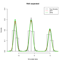
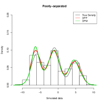
$\sigma=0.5$	$\sigma=1.5$

Figure 2: Simulation: DPP mixture model. The upper panel shows the histograms of two simulated datasets with true density (black), estimated density by DPP prior (red) and DPM prior (green). The lower panels present the histograms of the estimated number of clusters by DPP prior (2nd row) and DPM prior (3rd row).

We carry out two simulation studies to evaluate the performance of the repulsive DPP prior in clustering and density estimation, with both univariate and multivariate responses. Results are summarized in Figure 2. Details of the simulation setup and more results are shown in Web Appendix B. See there also for more discussion of Figure 2 and for a statement of the multivariate version of the DPP mixture model. The results show that the DPP prior leads to a sparser representation with interpretable clusters compared to DPM, while maintaining a good fit for the density estimate, making it a preferable prior model for applications where such parsimony is desired.

4.2 KIRC Protein Data Analysis

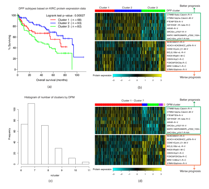
Figure 3: KIRC data. Panel (a) shows a Kaplan-Meier plot of overall survival in the KIRC core set stratified by three clusters identified under DPP prior. Panel (b) shows the top differentially expressed protein markers among three DPP clusters. Columns correspond to patients, rows correspond to proteins. Panel (c) is the histogram of the number of clusters identified under DPM prior. Panel (d) shows a heatmap of seven DPM clusters for top differentially expressed protein markers. The sizes of the seven clusters are 163, 19, 39, 14, 6, 1 and 1, respectively.

We implement inference under the proposed DPP mixture model for protein expression data from Yuan et al., (2014) with $n=243$ samples and $D=17$ protein markers for kidney renal clear cell carcinoma (KIRC). See equation (4) in Web Appendix A.2 for a statement of the DPP mixture model (4.1) with a multivariate normal kernel $p(y_{i}\mid\mu_{k})$. Inference goals include correlating protein expression with patients’ overall survival. The $n=243$ KIRC samples are classified into three clusters by the proposed DPP mixture model. As shown in Figure 3a, patients stratified by these three DPP groups exhibit very distinct survival patterns ($p$-value under a log-rank test is $p=0.00027$). Proteins that are correlated with better prognosis are relatively elevated in cluster 2 (the best survival group) while the proteins correlated with worst survival are relatively elevated in clusters 1 and 3 (especially cluster 3, the worst survival group) (Figure 3b). These results suggest that inference under the DPP prior can successfully classify patients into biologically meaningful groups based on molecular profiles.

In contrast, under the DPM mixture model, $K=7$ clusters are identified, estimated as the mode of $p(K\mid\bm{y})$ shown in Figure 3c. Most of the seven clusters have small size ($<$ 20) while 2/3 of the samples are allocated to one cluster (the red bar in Figure 3d). The clusters are not easily interpreted (Figure 3d).

In summary, inference under the DPP prior provides fewer clusters and gives more interpretable results in molecular profile-based classifications than inference under a comparable DPM prior.

5 A DPP Feature Allocation Model

5.1 Motivation and Model

Breast cancer is a heterogeneous disease in terms of molecular alterations and clinical responses. Gene expression profiling can provide valuable information for understanding this complexity and consequently for predicting clinical outcomes. Here we consider a study reported in Chen et al., (2013) who aim to characterize gene expression profiles by a small number of underlying distinct molecular drivers. These latent molecular drivers should be linked to different subsets of samples. This motivates us to propose the model below which formalizes this preference by using a DPP prior for the pattern of how molecular drivers (the columns of the matrix $Z$ below) are linked to samples (rows of $Z$). Let $Y$ denote the observed $n\times S$ data matrix with rows representing samples and columns representing genes. Let $Z$ be an $n\times K$ binary matrix with $z_{ik}=1$ if molecular driver $k$ presents in sample $i$, and 0 otherwise. That is, the $k$-th column $\bm{z}_{k}$ defines the subset $G_{k}=\{i:\;z_{ik}=1\}$ of samples that are linked with the $k$-th molecular driver. The entire matrix $Z$ defines a multiset $\{G_{k},\;k=1,\ldots,K\}$. Such multisets are known as feature allocation (Broderick et al., 2013b, ) and are popular tools in machine learning to implement inference about overlapping subsets of experimental units (customers etc.). The special case of non-overlapping subsets that cover all samples, that is, $G_{k}\cap G_{\ell}=\emptyset$ and $\bigcup G_{k}=\{1,\ldots,n\}$, is a partition. See Broderick et al., 2013a for a recent review. We use the feature allocation matrix $Z$ to construct a sampling model for the breast cancer gene expression data $Y$:

$$Y=Z\bm{\beta}+E,$$ (5.1)

where $\bm{\beta}$ is a $K\times S$ loading matrix with each entry $\beta_{kj}$ weighing the contribution of gene $j$ to the driver $k$ and $E=[e_{ij}]$ is an error matrix with $e_{ij}\sim N(0,\sigma^{2})$, independently. This defines a sampling model for the observed gene expressions $Y$ in terms of assumed latent structure $Z$. That is, $y_{ij}\sim N\left(\sum_{k=1}^{K}z_{ik}\beta_{kj},\sigma^{2}\right).$

The key assumption in a feature allocation model is the prior model on $Z$. A technically convenient and traditional prior is the Indian buffet process (IBP) (Ghahramani and Griffiths,, 2006). One of the key properties of the IBP, in the context of this application, is the implied independence across columns of the binary matrix (re-arranging columns in left ordered form or by other constraints introduces a trivial form of dependence). This independence is undesirable for the desired inference on molecular drivers. In particular, independence across columns implies a positive prior probability for identical columns, which is meaningless in the interpretation of columns as distinct molecular drivers.

DPP feature allocation. In contrast to the IBP, a DPP prior on the columns $\bm{z}_{k}$ formalizes the desired parsimony in identifying latent molecular drivers. We assume

$$\{\bm{z}_{k},\;k=1,\ldots,K\}\sim\mbox{DPP}(C)\mbox{ with }C(\bm{z}_{\ell},\bm{z}_{\ell^{\prime}})=\exp\left\{-\frac{\sum_{i=1}^{n}(z_{i\ell^{\prime}}-z_{i\ell})^{2}}{\theta^{2}}\right\}.$$ (5.2)

With large $n$, there is no effective way to decompose the kernel matrix $C$ ($N\times N$ matrix with $N=2^{n}$) and to compute the eigenvalues and the corresponding eigenvectors. We therefore fix $\theta$ in (5.2) and complete the model with a conditionally conjugate prior on the coefficients, $\beta_{kj}\mathrel{\mathop{\sim}\limits^{\mbox{\footnotesize i.i.d.}}}N(0,\tau^{2})$, and hyperpriors $1/\sigma^{2}\sim\mbox{Ga}(a_{0},b_{0}),1/\tau^{2}\sim\mbox{Ga}(a_{1},b_{1}).$

DPP-$K$ feature allocation. In the upcoming applications we find it convenient to work with a slight variation of model (5.2). Let $\mbox{DPP}_{K}(C)$ denote a DPP prior restricted to a fixed number of atoms, $K$, and define

$$\{\bm{z}_{k},\;k=1,\ldots,K\}{\mid K}\sim\mbox{DPP}_{K}(C)\mbox{ and }K\sim p(K)$$ (5.3)

for some prior $p(K)$. We refer to the model as the DPP-$K$ feature allocation model. The reason for introducing the DPP-$K$ model is that it facilitates a computationally efficient posterior simulation scheme. Under (5.2) we require a RJ type implementation, following the general scheme in Section 3.2. However, in some applications it is difficult to construct proposal distributions that lead to reasonably mixing Markov chains. Instead we propose in Web Appendix C an alternative MCMC scheme under (5.3), which we find to work well for applications with feature allocation problems. Posterior inference in model (5.2) as well as in (5.3) is implemented by MCMC posterior simulation. Details are shown in Web Appendix C.

Simulation study.

We carry out a simulation study to compare inference under the DPP-$K$ feature allocation prior versus the IBP prior. Results are summarized in Figure 4. More discussion of the results and details of the simulation setup are in Web Appendix D. With fewer latent features, inference under the DPP prior can better and more parsimoniously recover the simulation truth than under a standard IBP prior in this simulated example.

5.2 Breast Cancer (BRCA) Data Analysis

We analyze the TCGA BRCA mRNA expression data (The Cancer Genome Atlas Network et al.,, 2012). We focus on $n=150$ tumor samples classified as basal-like, HER2-enriched (HER2) and luminal A (LumA) subtypes by PAM50, a well-established 50-gene signature for distinguishing the gene expression-based “intrinsic” subtypes of breast cancer (Parker et al.,, 2009). Among those three subtypes, the HER2-enriched subtype is well studied. There are effective therapeutic drugs developed for targeting HER2 breast cancer. The basal-like subtype (also known as triple-negative breast cancer due to its lacking of expression of estrogen receptor (ER), progesterone receptor (PR) and HER2), and the LumA subtype, which is known to have lowest overall mutation rate, are poorly understood. As a result, there is currently no effective targeted therapy for these two subtypes, leaving chemotherapy as the main therapeutic treatment. A better characterization of basal-like and LumA subtypes at the molecular level is needed for clinical studies.

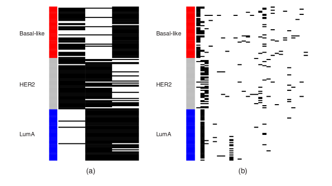
Figure 5: BRCA data. Estimated feature allocation matrix $\hat{Z}$ under the DPP prior (panel a) and under the IBP prior (b).

We implement inference under the proposed DPP-$K$ latent feature model and identify $K=3$ latent features. Figure 5a shows the posterior inferred latent feature matrix $Z$ with different breast cancer subtypes samples marked by different colors on the left. The basal-like, HER2 and LumA samples show clear and distinct patterns: 35 of 50 basal-like samples exhibit the first and third features and 44 of 50 are depleted with respect to the second feature; 43 of 50 HER2 samples exhibit the first two features and 33 of 50 are depleted with respect to the third feature; 48 of 50 LumA samples exhibit the second and third features and 47 of 50 are depleted with the first feature. More biological findings are discussed in Web Appendix E.

For comparison, we analyze the same BRCA dataset under a model with an IBP prior. It identifies 27 latent features, of which 17 are active in less than 4 samples. Figure 5b shows the estimated latent feature matrix $Z$. The first three features identified under the IBP prior can distinguish different breast cancer subtypes: 44 of 50 basal-like samples exhibit the first feature; 4 of 50 HER2 samples and none of LumA samples exhibit the first feature; 48 of 50 LumA samples exhibit the third feature. However, for the remaining 24 features, we can not observe any pattern for different breast cancer subtypes: these features were sparsely scattered across all samples. This is a good example of how the independent prior across features, as it is implied in the IBP model, leads to a lack of parsimony and difficult interpretability in the latent structure. In summary, the DPP prior model provides a less complicated representation and more interpretable features than inference under the IBP prior model.

6 Conclusions

We argue for the use of repulsive priors in models that involve latent structure as the main inference target. In many such problems interpretation of the imputed latent structure favors diverse and parsimonious choices. We specifically discuss examples involving inference for mixture models and feature allocation models. In these settings, commonly used models assume independence across latent clusters, features etc., which is technically convenient, but often inappropriate for the desired inference. We instead propose the use of DPP models as repulsive priors. The DPP model is attractive mainly because of the availability of easy to implement posterior simulation schemes.

We compare inference using DPP priors with standard Bayesian nonparametric priors in the cluster analysis of renal clear cell carcinoma and a feature allocation analysis of TCGA BRCA mRNA expression data. Our examples show that using DPP priors leads to posterior inference that gains substantially in parsimony and interpretability. Our case study results are methodologically corroborated by our analysis of the inferred structures. Also, DPP priors lead to a noticeable reduction in model uncertainty and, consequently, significantly more efficient estimators of latent structures.

Beyond mixture models and feature allocation models, inference for latent structures arises naturally in many other biomedical applications. One class of such examples are applications that involve nested clustering, that is, clustering of one set of experimental units (e.g., proteins) with respect to shared nested partitions on another set of experimental units (e.g., patients). Lee et al., (2013) discussed such applications, but with independent priors across distinct nested partitions. In some contexts, the latent structure of interest could be a graph, for example, a conditional independence graph that might be shared across some subpopulations. For example, Mitra et al., (2015) considered dependence structure of histone modifications across different conditions.

Several important limitations remain. In some applications repulsive priors are inappropriate. For example, inference for tumor heterogeneity might involve a prior across latent hypothetical subclones. However, following the notion of a phylogenetic tree of tumor cell subpopulations, some of these latent subclones should differ by few features (mutations, copy number variations etc.) only. Also, important computational limitations may be encountered, depending on specific applications. For example, in big data settings, fast posterior approximations developed for standard prior models may not extend directly to the case of DPP priors (Xu et al.,, 2015). Finally, problems related to label-switching (Jasra et al.,, 2005) remain an issue like in any mixture model. This is the case because the DPP prior remains exchangeable, for example across the $\mu_{k}$ in the mixture model (4.1).

7 Supplementary Materials

Web appendices and figures referenced in Sections 4.1, 5.1 and 5.2 are available with this paper at the Biometrics website on Wiley Online Library.

(a) True $Z^{o}$	(b) Estimated $\hat{Z}$ by DPP	(c) Estimated $\hat{Z}$ by IBP
(d) True $\bm{\beta}^{o}$	(e) Estimated $\hat{\bm{\beta}}$ by DPP	(f) Estimated $\hat{\bm{\beta}}$ by IBP
	(g)	(h)

Figure 4: Simulation: DPP feature allocation model. Panels (a-c) show the true feature allocation matrix $Z^{o}$ and the estimate $\hat{Z}$ under the DPP prior and the IBP prior, respectively. Panels (d-f) show the true feature mean $\bm{\beta}^{o}$ and the estimated $\hat{\bm{\beta}}$ under the DPP prior and under the IBP prior, respectively. Panels (g-h) are histograms of the number of latent features identified under DPP prior and IBP prior, respectively.

References

- Affandi et al., (2013) Affandi, R. H., Fox, E., and Taskar, B. (2013). Approximate inference in continuous determinantal processes. In Advances in Neural Information Processing Systems, pages 1430–1438.
- (2) Broderick, T., Jordan, M. I., Pitman, J., et al. (2013a). Cluster and feature modeling from combinatorial stochastic processes. Statistical Science, 28(3):289–312.
- (3) Broderick, T., Pitman, J., Jordan, M. I., et al. (2013b). Feature allocations, probability functions, and paintboxes. Bayesian Analysis, 8(4):801–836.
- Chen et al., (2013) Chen, M., Gao, C., and Zhao, H. (2013). Phylogenetic Indian buffet process: Theory and applications in integrative analysis of cancer genomics. arXiv preprint arXiv:1307.8229.
- Cocosco et al., (1997) Cocosco, C. A., Kollokian, V., Kwan, R. K.-S., Pike, G. B., and Evans, A. C. (1997). Brainweb: Online interface to a 3D MRI simulated brain database. In NeuroImage, volume 5, page 425. Citeseer.
- DeCarli et al., (1992) DeCarli, C., Maisog, J., Murphy, D. G., Teichberg, D., Rapoport, S. I., and Horwitz, B. (1992). Method for quantification of brain, ventricular, and subarachnoid CSF volumes from MR images. Journal of Computer Assisted Tomography, 16(2):274–284.
- Geyer and Møller, (1994) Geyer, C. J. and Møller, J. (1994). Simulation Procedures and Likelihood Inference for Spatial Point Processes. Scandinavian Journal of Statistics, 21(4):359–373.
- Ghahramani and Griffiths, (2006) Ghahramani, Z. and Griffiths, T. L. (2006). Infinite latent feature models and the Indian buffet process. In Advances in Neural Information Processing Systems, pages 475–482.
- Ghoshal, (2010) Ghoshal, S. (2010). The Dirichlet process, related priors and posterior asymptotics. In Hjort, N. L., Holmes, C., Müller, P., and Walker, S. G., editors, Bayesian Nonparametrics, pages 22–34. Cambridge University Press.
- Green, (1995) Green, P. J. (1995). Reversible jump Markov chain Monte Carlo computation and Bayesian model determination. Biometrika, 82:711–732.
- Jasra et al., (2005) Jasra, A., Holmes, C. C., and Stephens, D. A. (2005). Markov chain Monte Carlo methods and the label switching problem in Bayesian mixture modeling. Statistical Science, 20(1):50–67.
- Kingman, (1992) Kingman, J. F. C. (1992). Poisson Processes. Oxford University Press.
- Kulesza and Taskar, (2010) Kulesza, A. and Taskar, B. (2010). Structured determinantal point processes. In Advances in Neural Information Processing Systems, pages 1171–1179.
- Kulesza and Taskar, (2012) Kulesza, A. and Taskar, B. (2012). Determinantal point processes for machine learning. Machine Learning, 5(2-3):123–286.
- Kwok and Adams, (2012) Kwok, J. T. and Adams, R. P. (2012). Priors for diversity in generative latent variable models. In Advances in Neural Information Processing Systems, pages 2996–3004.
- Lavancier et al., (2015) Lavancier, F., Møller, J., and Rubak, E. (2015). Determinantal point process models and statistical inference. Journal of the Royal Statistical Society: Series B (Statistical Methodology), 77(4):853–877.
- Lee et al., (2013) Lee, J., Müller, P., Zhu, Y., and Ji., Y. (2013). A nonparametric Bayesian model for local clustering. Journal of the American Statistics Association, 108:775–788.
- Macchi, (1975) Macchi, O. (1975). The coincidence approach to stochastic point processes. Advances in Applied Probability, pages 83–122.
- Mitra et al., (2015) Mitra, R., Müller, P., and Ji, Y. (2015). Bayesian graphical models for differential pathways. Bayesian Analysis, to appear.
- Parker et al., (2009) Parker, J. S., Mullins, M., Cheang, M. C., Leung, S., Voduc, D., et al. (2009). Supervised risk predictor of breast cancer based on intrinsic subtypes. Journal of Clinical Oncology, 27(8):1160–1167.
- Petralia et al., (2012) Petralia, F., Rao, V., and Dunson, D. B. (2012). Repulsive mixtures. In Advances in Neural Information Processing Systems, pages 1889–1897.
- Rousseau and Mengersen, (2011) Rousseau, J. and Mengersen, K. (2011). Asymptotic behaviour of the posterior distribution in overfitted mixture models. Journal of the Royal Statistical Society: Series B (Statistical Methodology), 73(5):689–710.
- The Cancer Genome Atlas Network et al., (2012) The Cancer Genome Atlas Network et al. (2012). Comprehensive molecular portraits of human breast tumours. Nature, 490(7418):61–70.
- Xu et al., (2015) Xu, Y., Müller, P., Yuan, Y., Gulukota, K., and Ji, Y. (2015). MAD Bayes for tumor heterogeneity – feature allocation with exponential family sampling. Journal of the American Statistical Association, 110(510):503–514.
- Yuan et al., (2014) Yuan, Y., Van Allen, E. M., Omberg, L., Wagle, N., et al. (2014). Assessing the clinical utility of cancer genomic and proteomic data across tumor types. Nature Biotechnology, 32(7):644–652.
- Zhu et al., (1998) Zhu, H., Williams, C., Rohwer, R., and Morciniec, M. (1998). Gaussian regression and optimal finite dimensional linear models. NATO ASI Series. Series F: Computer and System Sciences, pages 167–184.