Reducing the Candidate Line List for Practical Integration of Switching into Power System Operation

Abstract

Optimized operation of the transmission network is one solution to supply extra demand by more efficient use of transmission facilities, and line switching is one main tool to achieve this goal. In this paper, we add extra constraints to OPF formulation to limit the maximum number of switching operations in every hour based on network conditions, and add switching cost in the objective function to represent extra maintenance cost as a result of frequent switching. We also propose an algorithm to remove less important lines for switching in different loading conditions, so OPF with transmission switching will be solved faster for real-time operation. It is applied to a case study with several operation hours.

Nomenclature

Sets and Indices:
$N_{b}$: Set of buses with index i, k, n
$N_{g}$: Set of all generators with index g
$N_{l}$: Set of all lines (existing and candidate) with index l, m
$L_{k}$: Set of lines connected to bus k
$G_{k}$: Set of all generators connected to bus k with index ${k}$
$W_{k}$: Set of wind generators connected to bus k with index ${k}$
$T$: The length of time window with index t
$|\;\;|$: Size of a set
Parameters:
$q_{i}$: Per MWh load curtailment penalty at bus $\it i$
$Co_{g}^{t}$: Per MWh operation cost for generator $g$ in load block $t$
$\zeta_{l}$: Per switching cost for line $\it l$
$d_{i}^{t}$: Demand at bus $\it i$ in load block $\it t$
$B$: Diagonal matrix of line admittance
$Y$: Reduced admittance matrix (column and row related to reference bus are removed)
$\Psi$: Reduced bus-branch incidence matrix (row related to reference bus is removed)
$P_{g}^{max,t}$: Maximum capacity of generator $\it g$ in load block $t$
$P_{g}^{min,t}$: Minimum capacity of generator $\it g$ in load block $t$
$f_{l}^{max}$: Maximum capacity of line $\it l$
$f_{l}^{min}$: Minimum capacity of line $\it l$
$M_{l}$: Big $\it M$ is a large positive number for line $\it l$
$PTDF$: Power transfer distribution factor
$LODF$: Line outage distribution factor
Decision Variables:
$\delta_{l}$: Binary decision variable for switching line $\it l$
$r_{i,c}^{t}$: MW load curtailment at bus $\it i$ under operation state $c$ in load block $\it t$
$p_{g}^{t}$: Output power of generator $\it g$ in load block $\it t$
$f_{l,c}^{t}$: Power flow in line $\it l$ under operation state $c$ in load block $\it t$
$\theta_{i,c}^{t}$: Voltage angle at bus $\it i$ under operation state $c$ in load block $\it t$. $\Delta\theta_{l,c}^{t}$ is voltage angle difference across line $\it l$ under operation state $c$ in load block $\it t$, $\Delta\theta_{l,c}^{t}$= $\theta_{k,c}^{t}$-$\theta_{n,c}^{t}$ for line $\it l$ from bus $\it k$ to bus $\it n$.

1 Introduction

1.1 Why Switching?

Switching in power system is not a new concept and it used from the early formation of power system until now. During the time, the purpose of transmission switching is expanded. In this paper, we categorized the main purposes of transmission switching into three main categories:

• Corrective Action:
  Applying switching to clear fault and isolate affected equipment is the primary purpose of installing circuit breakers in power systems.

• Preventive Action:
  Reliability switching to back the system to normal condition and prevent load shedding and cascading failures are preventive actions that are applied by system operators usually after occurring a contingency in the network.

• Economic Purpose:
  In the recent decade, using transmission switching to decrease operation costs by managing congestions/network reconfiguration under normal operating conditions is investigated in literature. Therefore, we should expect more switching in power system in the future.

1.2 Literature review

There are extensive literature on transmission switching with different purposes. In this paper, we briefly review some of them.

• Switching for improving reliability
  Mazi et al. in [1] used transmission switching and bus-bar splitting as preventive actions that can help revealing overloads in lines and preventing cascading failures. In [2], Shao et al. incorporated line, bus-bar and shunt element switching into an algorithm for mitigating voltage violations and line overloads in system. Other related papers in this area: [3]–[5]

• Switching for loss reduction and congestion management
  Fliscounakis et al. in [6] used piece-wise linear approximation technique to linearize network losses representation in their mixed integer programming formulation. They considered line switching and phase shifter tap changing as tools to manage flows in lines and reduce losses. Authors in [7] used transmission switching and network topology reconfiguration as a tool for congestion management and preventing load shedding. They solved the problem using with both MIP formulation and generic algorithm. There are other options for congestion management in the network like suing FACTS devices and phase shifter transformers. Other related papers in this area: [8]–[12]

• Switching for topology optimization/Cost-benefit analysis
  Ruiz et al. in [13] proposed shift factor MIP formulation for topology control. Line opening is modeled with flow cancellation technique. This formulation is compact and its size depends on the size of monitoring and switchable lines. They deployed this technique for transmission planing as well. Hedman et al. in [14] evaluated the impact of transmission switching on nodal prices, load payments, generation revenues, and flowgate prices. There are several other works by Hedman and his group in this area that are cited in the other related papers section for further reading. In [15], Wu et al. Developed a heuristic method for transmission switching that integrated different criteria such as limiting violations of line flows, congestion rents, and production costs. They used Locational Marginal Price (LMP) for decision making in their heuristic method. Other related papers in this area: [16]–[20]

In this paper we would like to highlight the following concerns for transmission switching for economic purpose:

• Can we implement the selected switching plan in real networks?

• Can we solve the problem for large scale systems for real-time operation?

The rest of the paper is organized as follows: in section 2, technical issues related to switching is reviewed. It is followed by the proposed method and mathematical formulation in section 3. Section 4 has numerical results and the paper is concluded in section 5.

2 An Overview of Technical Issues related to Switching

Usually in transmission switching (TS) for economic purposes, steady-state of power system is formulated for TS optimization problem. Based on market intervals, it is a correct assumption for economic purposes. However, from practical (and reliability) perspective, steady-state analysis is not enough for a TS planning to be implemented. Moreover, switching is not a free action and the extra cost as a result of frequent switching should also be considered. In this section, the transient impact of switching, protection system misoperation, and circuit breaker maintenance is reviewed.

2.1 Transient impact of switching

Opening a transmission line or energizing a transformer will have some transient effects on voltage profile in the system that may trigger cascading failures. In Figure 1 (a), transient over voltage as a result of opening a transmission line is shown. The magnitude of this over-voltage may exceed 2 [P.U.] which is much higher than the accepted voltage deviation (1.05–1.1 [P.U.])during normal operation (steady-state). Figure 1 (b) shows the harmonics in voltage as a result of energizing a transformer. These transient phenomena may result in power system protection unnecessary operation that causes some problems for system reliability. Therefore, they should be considered in switching planning (directly or indirectly).

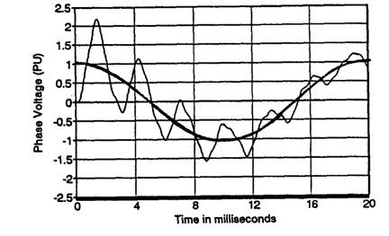
(a) Line Switching Voltage Transient

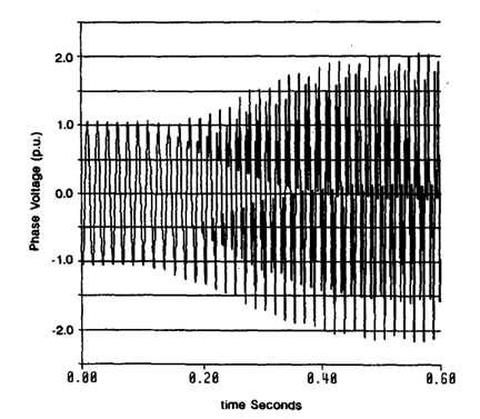
(b) Transformer Energizing Voltage Harmonics

Figure 1: Transient impact of switching [21]

2.2 Protection system misoperation

Power system protection schemes are mostly designed for static network configurations, and network reconfiguration may result in protection system misoperation. In Figure 2 protection system misoperation in ERCOT from 2011 to 2013 is shown. Adding frequent switching to power system operation will change network configuration more significantly (compared to the case with reliability switching only), therefore it most likely will increase such misoperation if the protection schemes cannot adapt themselves with network reconfiguration (which is the case in many power systems now).

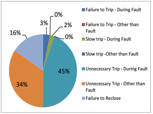
(a) By Category

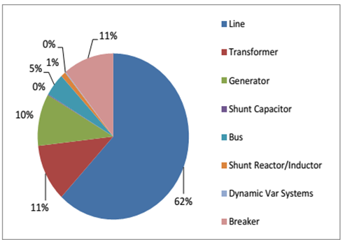
(b) By Equipment Protected

Figure 2: Protection System Misoperation Data ERCOT 2011-2013 [22]

2.3 Circuit breaker maintenance

As circuit breakers have a limit on the total number of switching before each maintenance, its cost should be considered in switching planning. A SIEMENS circuit breaker switching curve is shown in Figure 3. Based on this figure, total number of switching before maintenance is 6000 if the breaker opens a circuit under normal condition, and this number will decrease by increasing the current that should be cut by the beaker. For example, if this breaker opens 40KA short circuit current for 10 times it will need maintenance services. Equation (1) shows how to calculate the number of remaining switching for this breaker depending on the current ($I_{x}$). $k_{i}$ and $k_{x}$ can be found from Figure 3 based on current $I_{i}$ and $I_{x}$ respectively.

Number of remaining switching before next inspection/maintenance [23]:

$$n_{x}=\frac{6000-\sum\limits_{i=1}^{m}(n_{i}\times k_{i})}{k_{x}}$$ (1)

where:
$k_{i}$: weighting factor for $I$
$k_{x}$: weighting factor for $I_{x}$
$n_{i}$: number of performed interruptions at $I$
$n_{x}$: number of permissible interruptions at $I_{k}$

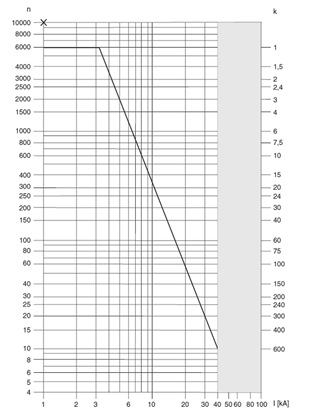
Figure 3: Number of switching vs. switching current [23]

In summary, technical issues related to transmission switching should also be considered as a part of planning for switching to be practical.

3 Modeling and Formulation

3.1 Proposed Algorithm

In this paper we have added the following constraints to the classic switching planning problem to make it more practical:

• Adding switching costs to the objective function.

• Considering a time window (T hours) to plan for switching rather than a single hour in real-time.

• Limiting the number of times that a line can be switched in the planning time window.

• Limiting total number of switching per hour in the network.

As running transient analysis and evaluating the impact of network reconfiguration on protection schemes are computationally expensive, we added last two constraints to integrate expert knowledge into our optimization formulation for limiting the number of switching in a way to be applicable in the system.

Solving switching optimization problem with extra constraints is challenging for large scale power systems especially that it should be run in real-time. We proposed a heuristic method to decrease the search space for making decision about switching. The proposed algorithm is summarized in the following steps:

Step 1

: Solve OPF for next T hours

Step 2

: Create Monitored Lines List (MLL)
MLL includes lines that their loading without switching is more than $\alpha\%$.

Step 3

: Calculate LODF for MLL for all closed lines

Step 4

: Reduce switching lines list
In this step, lines that their opening will cause overload in lines in MLL will be removed from switching list, as they will have negative impact on monitored lines.

Step 5

Solve OPF with reduced switching list

As mentioned above, this method is heuristic, as we do not consider multiple line switching in steps 3 and 4. Therefore we cannot guarantee optimality, and the answer will be sub-optimal. However, reducing the switching lines list will reduce computational time.

3.2 Mathematical Formulation

Transmission switching optimization problem formulation is given in (2)–(11). The objective function (2) includes load shedding penalty cost, electricity generation cost and cost related to switching. In this formulation we penalize breakers operation for both line opening and closing, but it is possible to limit it to line opening if it is preferred. Equations (3)–(9) represent standard constraints for optimal power flow with line switching binary variable $\delta$. Equations (10) and (11) are two new constraints that are added to integrate expert knowledge into the optimization problem. Equation (10) limits total number of switching for a line during next T hours, and equation (11) limits total number of switching in the system in every hour. The right hand side of these equations will be set by system operators based on the network configuration and loading condition.

$$Z^{*}{=} \min\limits_{\boldsymbol{p},\boldsymbol{\theta},\boldsymbol{r},\boldsymbol{f},\boldsymbol{\delta}}\sum\limits_{T}\big{[}\sum\limits_{N_{b}}q_{i}r_{i}^{t}{+}\sum\limits_{Ng}Co_{g}^{t}p_{g}^{t}+\sum\limits_{N_{l}}\zeta_{l}|\delta^{t}_{l}-\delta^{t-1}_{l}|\big{]}$$ (2)

$$\mathrm{st.}\quad {-}\sum\limits_{L_{k}}f_{l}^{t}{+}\sum\limits_{G_{k}}p^{t}_{g}{+}r_{k}^{t}{=}d_{k}^{t},\hfill\forall t,k$$ (3)

$${-}M_{l}(1-\delta^{t}_{l})\leq f_{l}^{t}{-}B_{l,l}\Delta\theta_{l}^{t},\hfill\forall t,l$$ (4)

$$M_{l}(1-\delta^{t}_{l})\geq f_{l}^{t}{-}B_{l,l}\Delta\theta_{l}^{t},\hfill\forall t,l$$ (5)

$$(\delta^{t}_{l})f_{l}^{min}\leq f_{l}^{t}\leq f_{l}^{max}(\delta^{t}_{l}),\hfill\forall t,l$$ (6)

$$0\leq r_{i}^{t}\leq d_{i}^{t},\hfill\forall t,i$$ (7)

$${-}\frac{\pi}{2}\leq\theta_{i}^{t}\leq\frac{\pi}{2},\hfill\forall t,i$$ (8)

$$P_{g}^{min,t}\leq p_{g}^{t}\leq P_{g}^{max,t},\hfill\forall t,g$$ (9)

$$\sum\limits_{T}|\delta^{t}_{l}-\delta^{t-1}_{l}|\leq H1_{l},\forall l$$ (10)

$$\sum\limits_{N_{l}}|\delta^{t}_{l}-\delta^{t-1}_{l}|\leq H2^{t},\forall t$$ (11)

Equations (12) and (13) are used to create monitored lines list. MLL contains lines with more than $\alpha\%$ loading.

$$Viol_{l}^{t}=f_{l}^{t}-\alpha\times f_{l}^{max},\forall l,t$$ (12)

$$MLL=\{l\in N_{l}\,|\,Viol_{l}^{t}>0,\forall t\}$$ (13)

To calculate LDOF and post switching line flows, equations (14)–(17) are used [24].

$$PTDF_{l,l}=B_{l,l}\Psi_{l}^{T}[Y]^{-1}\Psi_{l}$$ (14)

$$PTDF_{m,l}=B_{m,m}\Psi_{m}^{T}[Y]^{-1}\Psi_{l}$$ (15)

$$LODF_{m,l}=PTDF_{m,l}(1-PTDF_{l,l})^{-1}$$ (16)

$$f_{m,l}^{t}=f_{m}^{t}+LODF_{m,l}f_{l}^{t}$$ (17)

Switching Lines List $SLL$ is reduced by using equations (18) and (19).

$$SLL_{E}=\{l\in N_{l}\,|\,f_{m,l}^{t}-f_{m}^{max}\geq 0,\forall m\in MLL\}$$ (18)

$$SLL_{u}=SLL_{o}\setminus SLL_{E}$$ (19)

4 Case study and numerical results

All illustrated results in this section have been obtained from a personal computer with 2.0-GHz CPU using MATLAB R2014a [25] and YALMIP R20140221 package [26] as a modeling language and GUROBI 5.6 [27] as the solver. Two different case studies consisting of 13-bus system and reduced ERCOT network with 317-bus are considered.

4.1 13-bus system

This 13-bus system is a simplified version of the ERCOT network that is developed for educational purposes (see Figure 4). This case study has 13 buses, 33 branches, 16 power plants, and 9 load centers [24]. The parameters are set as following:

• Next 5 hours is considered for switching planning ($T=5$).

• $H1_{l}=2$.

• $H2^{t}=4$.

• $|N_{l}|=34$.

• $\alpha=50\%$.

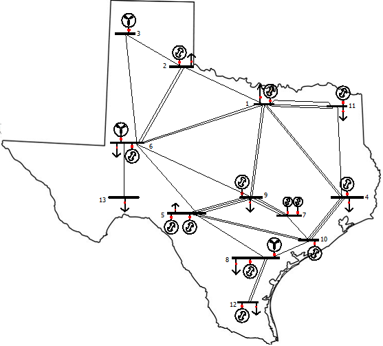
Figure 4: 13-bus system [24]

In the first step, transmission switching (TS) is solved without any extra constraints defined in this paper (classic TS). The selected TS plan is shown in Figure 5. Operation cost saving as a result of switching is 0.12% compared to the base case without any switching. Without any extra constrains, the system operator should switch 44 times during next 5 hours in a network with 34 lines. Lines 8 and 33 are switched 5 times during 5 hours. 12 times switching in hour 5 will significantly change system configuration and may affect protection system performance that makes such switching plans impractical.

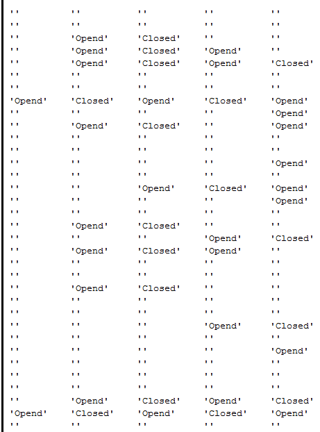
Figure 5: Switching plan for next 5 hours

By adding extra constraints (still not using MLL and SLL), the total number of switching will reduce to 18 (shows 144% switching reduction). However, this less switching will result in less saving and some extra operation costs compared to the TS without any extra constraint. For this case study, this extra cost is 0.021%. Figure 6 (a) shows the switching plan for next 5 hours after adding extra constraints. As we didn’t use our proposed heuristic method until now, this TS is optimal.

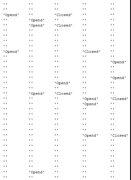
(a)

Figure 6: Switching plan with (a) and without (b) extra constrains

In the next step, we create MLL and SLL based on equations in section 3. As shown in Table 1, the number of monitored lines and the lines eligible for switching change from time to time based on network loading condition.

Table 1: Size of MLL and updated Switching Lines List ($SLL_{u}$)

	t=1	t=2	t=3	t=4	t=5
$|MLL|$	8	9	10	6	7
$|SLL_{u}|$	18	11	3	11	23

TS optimization problem is solved with $SLL_{u}$ instead of $SLL_{o}$, and the result is shown in Figure 6 (b). By comparing figures (a) and (b), it is clear that TS after applying MLL and SLL is no longer optimal, and the extra operation cost is 0.0118% for this case. However, the simulation time is reduced from 271.67 seconds to 2.1 seconds that shows more than 129 times simulation time reduction. Moreover, the number fo switching is reduced by 80%. Therefore, using the proposed heuristic method is a trade-off between optimality and simulation time.

4.2 Reduced ERCOT System

A reduced model of the ERCOT system is provided in [28]. This network contains 317 buses, 427 branches, 489 conventional power plants, 36 wind farms and 182 load centers. The purpose of developing this case was to evaluate the impact of large penetration of wind in Competitive Renewable Energy Zone (CREZ) area on ERCOT market and transmission expansion requirements to transfer wind power to central and east Texas. For this reason, west Texas is simulated in detail, and the rest of the ERCOT area is aggregated to three zones as delivery points of CREZ. Parameters are set as follows:

• T=3.

• $H1_{l}$=2.

• $H2^{t}$=8.

• $\alpha=50\%$.

MLL and SLL for this case study are shown in Table 2. As shown in the second row, updated switching lines list $SLL_{u}$ contained much less lines compared to original switching lines list ($|SLL_{o}|=427$) that will reduce computational time significantly.

Table 2: Size of MLL and updated Switching Lines List ($SLL_{u}$)

	t=1	t=2	t=3
$|MLL|$	42	42	43
$|SLL_{u}|$	91	97	63

Here is a summary of results:
Operation cost saving as a result of applying TS for the case w/o extra constraints on switching: 5.1%
Extra cost as a result of adding new constraints: 2.1% (3% saving on operation costs)
Number of switching w/o extra constraints: 308 (22 lines are switched 3 times each)
Number of switching w/ extra constraints: 23 (1239% switching reduction)
Simulation time w/o MLL and SLL: no answer after 2 days
Simulation time w/ MLL and SLL: 33 mins

This case study shows the impact of the proposed heuristic method on reducing the computational time.

5 Conclusion

In summary:

• Adding some extra constraints may not significantly decrease the benefits of transmission switching, but can significantly decrease the total number of switching that benefits system reliability.

• Considering multiple hours for TS planning with switching costs may prevent frequent switching of a small group of lines.

As a part of our future work:

• Developing algorithms to decrease computational time for large scale systems

• Integrating network losses and reactive power requirements

• Integrating $N-1$ contingency analysis into transmission switching as power system should be operated in a way that satisfies $N-1$ criterion.

References

- [1] A. Mazi, B. Wollenberg, and M. Hesse, “Corrective control of power system flows by line and bus-bar switching,” Power Systems, IEEE Transactions on, vol. 1, no. 3, pp. 258–264, Aug 1986.
- [2] W. Shao and V. Vittal, “Corrective switching algorithm for relieving overloads and voltage violations,” Power Systems, IEEE Transactions on, vol. 20, no. 4, pp. 1877–1885, Nov 2005.
- [3] H. Glavitsch, “Switching as means of control in the power system,” International Journal of Electrical Power and Energy Systems, vol. 7, no. 2, pp. 92 – 100, 1985. [Online]. Available: http://www.sciencedirect.com/science/article/pii/0142061585900146
- [4] R. Bacher and H. Glavitsch, “Network topology optimization with security constraints,” Power Systems, IEEE Transactions on, vol. 1, no. 4, pp. 103–111, Nov 1986.
- [5] W. Shao and V. Vittal, “Bip-based opf for line and bus-bar switching to relieve overloads and voltage violations,” in Power Systems Conference and Exposition, 2006. PSCE ’06. 2006 IEEE PES, Oct 2006, pp. 2090–2095.
- [6] S. Fliscounakis, F. Zaoui, G. Simeant, and R. Gonzalez, “Topology influence on loss reduction as a mixed integer linear programming problem,” in Power Tech, 2007 IEEE Lausanne, July 2007, pp. 1987–1990.
- [7] G. Granelli, M. Montagna, F. Zanellini, P. Bresesti, R. Vailati, and M. Innorta, “Optimal network reconfiguration for congestion management by deterministic and genetic algorithms,” Electric Power Systems Research, vol. 76, no. 6–7, pp. 549 – 556, 2006. [Online]. Available: http://www.sciencedirect.com/science/article/pii/S0378779605002257
- [8] R. Bacher and H. Glavitsch, “Loss reduction by network switching,” Power Systems, IEEE Transactions on, vol. 3, no. 2, pp. 447–454, May 1988.
- [9] O. Ziaee and F. ch., “Thyristor-controlled switch capacitor placement in large-scale power systems via mixed integer linear programming and taylor series expansion,” in PES General Meeting — Conference Exposition, 2014 IEEE, July 2014, pp. 1–5.
- [10] M. Majidi Qadikolai and S. Afshania, “An approach to determine the revenue share of each facts device under deregulated environment,” Journal of Applied Sciences, pp. 1677–1685, 2009. [Online]. Available: http://www.docsdrive.com/pdfs/ansinet/jas/2009/1677-1685.pdf
- [11] O. Ziaee and F. ch., “Optimal location-allocation of facts devices on a transmission network,” Power Systems, IEEE Transactions on, 2015.
- [12] Q. M. Majidi, S. Afsharnia, M. S. Ghazizadeh, and A. Pazuki, “A new method for optimal location of facts devices in deregulated electricity market,” in Electric Power Conference, 2008. EPEC 2008. IEEE Canada, Oct 2008, pp. 1–6.
- [13] P. Ruiz, A. Rudkevich, M. Caramanis, E. Goldis, E. Ntakou, and C. Philbrick, “Reduced MIP formulation for transmission topology control,” in 2012 50th Annual Allerton Conference on Communication, Control, and Computing (Allerton), Oct. 2012, pp. 1073–1079.
- [14] K. Hedman, R. O’Neill, E. Fisher, and S. Oren, “Optimal transmission switching with sensitivity analysis and extensions,” IEEE Transactions on Power Systems, vol. 23, no. 3, pp. 1469–1479, Aug. 2008.
- [15] J. Wu and K. Cheung, “On selection of transmission line candidates for optimal transmission switching in large power networks,” in 2013 IEEE Power and Energy Society General Meeting (PES), Jul. 2013, pp. 1–5.
- [16] P. Ruiz, J. Foster, A. Rudkevich, and M. Caramanis, “Tractable transmission topology control using sensitivity analysis,” IEEE Transactions on Power Systems, vol. 27, no. 3, pp. 1550–1559, Aug. 2012.
- [17] R. O’Neill, R. Baldick, U. Helman, M. Rothkopf, and J. Stewart, W., “Dispatchable transmission in rto markets,” Power Systems, IEEE Transactions on, vol. 20, no. 1, pp. 171–179, Feb 2005.
- [18] K. Hedman, M. Ferris, R. O’Neill, E. Fisher, and S. Oren, “Co-optimization of generation unit commitment and transmission switching with n-1 reliability,” Power Systems, IEEE Transactions on, vol. 25, no. 2, pp. 1052–1063, May 2010.
- [19] K. Hedman, S. Oren, and R. O’Neill, “A review of transmission switching and network topology optimization,” in Power and Energy Society General Meeting, 2011 IEEE, July 2011, pp. 1–7.
- [20] M. Sahraei-Ardakani, A. Korad, K. Hedman, P. Lipka, and S. Oren, “Performance of ac and dc based transmission switching heuristics on a large-scale polish system,” in PES General Meeting — Conference Exposition, 2014 IEEE, July 2014, pp. 1–5.
- [21] M. M. Adibi, R. W. Alexander, and B. Avramovic, “Overvoltage control during restoration,” Power Systems, IEEE Transactions on, vol. 7, no. 4, pp. 1464–1470, Nov 1992.
- [22] Texas Reliability Entity, Inc., “2013 assessment of reliability performance for the electric reliability council of texas, inc. (ERCOT) region,” April 2014.
- [23] SIEMENS, “Type sps2-15.5/25.8/38/48.3/72.5kv-40ka, gas circuit breaker, spring operating mechanism, pb 3638-04.”
- [24] M. Majidi-Qadikolai and R. Baldick, “Integration of N-1 contingency analysis with systematic transmission capacity expansion planning: ERCOT case study,” IEEE Transactions on Power Systems, 2015.
- [25] MATLAB, version 8.3.0.532 (R2014a). Natick, Massachusetts: The MathWorks Inc., 2014.
- [26] J. Lofberg, “Yalmip : A toolbox for modeling and optimization in MATLAB,” in Proceedings of the CACSD Conference, Taipei, Taiwan, 2004. [Online]. Available: http://users.isy.liu.se/johanl/yalmip
- [27] Gurobi Optimization, Inc., “Gurobi optimizer reference manual,” 2014. [Online]. Available: http://www.gurobi.com
- [28] H. Park and R. Baldick, “Transmission planning under uncertainties of wind and load: Sequential approximation approach,” IEEE Transactions on Power Systems, vol. 28, no. 3, pp. 2395–2402, Aug 2013.