Modelling Structured Societies: a Multi-relational Approach to Context Permeability

Abstract

The structure of social relations is fundamental for the construction of plausible simulation scenarios. It shapes the way actors interact and create their identity within overlapping social contexts. Each actor interacts in multiple contexts within different types of social relations that constitute their social space. In this article, we present an approach to model structured agent societies with multiple coexisting social networks. We study the notion of context permeability, using a game in which agents try to achieve global consensus. We design and analyse two different models of permeability. In the first model, agents interact concurrently in multiple social networks. In the second, we introduce a context switching mechanism which adds a dynamic temporal component to agent interaction in the model. Agents switch between the different networks spending more or less time in each one. We compare these models and analyse the influence of different social networks regarding the speed of convergence to consensus. We conduct a series of experiments that show the impact of different configurations for coexisting social networks. This approach unveils both the limitations of the current modelling approaches and possible research directions for complex social space simulations.

‘

1 Introduction

In most simulations of complex social phenomena, agents are considered to inhabit a space in which structure is very simple. This space has little resemblance with the social world it is supposed to depict and for which conclusions are supposed to be extrapolated. This simplicity does not come by chance, rather, it is necessary and desired by the researchers: the problems to be approached are themselves so complex that whichever factors of complexity can be reduced (or at least postponed), the reduction is always welcome. So, it is common practice that geographical space is reduced to a two-dimensional grid, and all social relations between agents are condensed into one more or less structured abstract relation. Most social simulation and modelling approaches disregard the fact that we engage in multiple social relations. Moreover, each kind of social relation can possess distinctive characteristics that include: rich information such as degree of connectivity, centrality, trust, interactions frequency, asymmetry, and so on.

To explore the addition of multiple relations and its consequences for the dissemination of phenomena in social simulations, we put forward to reduce the emphasis given on agent individual interactions. We accomplished this by choosing a simple – and especially neutral – game to model those interactions. Our main concern was that the game itself would not provide biases or trends in the collective phenomenon being studied, so we chose the consensus formation game, with a straightforward majority rule to decide the outcome of each individual move.

While most models are simplified descriptions – reductions – of real-world phenomena, many constitute complex systems themselves and thus, we need techniques such as simulation to explore their properties. We can make a distinction between two types of complexity: the complexity of real systems (ontological complexity) and the complexity of models (descriptive complexity) [1]. The levels of abstraction in a simulation model can then range from data-driven paradigms to more abstract descriptions that allow us to create what-if-scenarios. The study of this abstract descriptive complexity in simulation models is as valuable as its data-driven counterpart. We may not be able to make predictions based on the direct application of such models; but, their study can inspire the engineering of artificial complex systems and reveal properties with applications beyond the explanation of observable phenomena. Studying consensus formation can thus advance our understanding of related real-world social phenomena.

Examples of thematic real-world phenomena in social simulation models include for instance the joint assessments of policies or, in the context of economics and politics, the voting problem. Herbert Simon’s investigations on this problem were one of the first stepping stones to the field of social simulation [2]; which then inspired models (like the one we present in this article) related to evolution and dissemination of opinions, which we call opinion dynamics. In agent-based opinion dynamics, agent interactions are guided by social space abstractions. In some models, the dimensionality and structure of this space is irrelevant (any agent can interact with any other agent). Other models use an underlying artefact that structures agent neighbourhoods. Axelrod for instance, represents agent neighbourhoods as a bi-dimensional grid in its model of dissemination of culture [3]. In an attempt to mimic real social systems, one can also make use of complex network models to create the infrastructure that guides agent interaction (see [4] for an example).

In real-world scenarios, actors engage in a multitude of social relations different in kind and quality. Most simulation models don’t explore social space designs that take into account the differentiation between coexisting social networks. Modelling multiple coexisting relations was an idea pioneered by Peter Albin in [5] but without further development. The process of interacting in these different complex social dimensions can be seen as the basis for the formation of our social identity [6, 7].

In this article, we explore the of modelling opinion dynamics with multiple social networks. We look at how the properties of different network models influence the convergence to opinion consensus. We present a series of models that use these networks in different ways: which create distinct emergent dynamics. We want to study the consequences of using multiple social networks at the same time while maintaining the interaction model as simple and abstract as possible (following the methodology in most opinion dynamics literature). We present two models where agents can: interact at the same time in the multiple networks (choosing partners from any network); or switch between networks (choosing only partners from their current network).

1.1 Article Structure

This article is organised as follows. In the next section, we present the work related to opinion dynamics, social space modelling and complex network models. In the following section, we describe our game of consensus and introduce our multiple model variations. These are designed to study the notion of context permeability and consensus formation in multiple social networks. Section 4 describes the experimental setup; the set of tool and methodologies followed to conduct our investigations. In section 5, we present and discuss our results and compare the different simulation models. Finally, we summarise what we learned from our experiments and point out future research directions.

2 Related Work

In this section, we present work related to opinion dynamics, social space modelling, and complex network models.

2.1 Opinion Dynamics and Consensus Formation

Formal opinion dynamics models provide an understanding, if not an analysis, of opinion formation processes. An early formulation of such models was created as a way to understand complex phenomena found empirically in groups [8]. The work on consensus building (in the context of decision-making) was first studied by DeGroot [9] and Lehrer [10]. Empirical studies of opinion formation in large populations have methodological limitations. Computational sociology arises with a set of tools – simulation models in particular – to cope with such limitations. We use multi-agent simulation (MAS) as a methodological framework to study such social phenomena in a larger scale. Most opinion dynamics models make use of binary opinion values [11, 12], or continuous values [13, 14]. For a detailed analysis over some opinion dynamics models, refer to [15].

Opinion dynamics models allow us to discover under which circumstances a population of agents reaches consensus or polarisation. Agent-based models can have broader application outside social simulation though. In computational distributed systems, consensus is a means by which processes agree on some data value needed during computation. Typically, this agreement is the result of a negotiation process (often with the aid of a mediator). In human societies, social conventions emerge to deal with coordination and subsequently with cooperation problems [16]. These conventions are regularities of behaviour that can turn normative if they come to be persistent solutions to recurrent problems. MAS are also capable of producing emergent conventions in coordination or cooperation problems [17]. The decentralised nature of these computational models of consensus is highly desirable for dynamic control problems. In these scenarios, creating conventions before hand (off-line), or developing a central control mechanism for generating them, can be a difficult and intractable task: either due to the uncertainty and complexity associated with the environment, or due to the system scale and heterogeneity (which makes it very difficult to handcraft each component).

Consensus models are also investigated as means to create conventions in MAS. Shoham and Tennenholtz create a bridge between economic literature and machine learning by studying a series of models in which multiple agents are engaged in learning a particular convention [18]. They call this process co-learning. The complexity of these systems comes from its concurrent nature: one agent adapts to the behaviour of another agents it has encountered, these other agents update their behaviour in a similar fashion, which results in a highly non-linear system dynamics. In their work, Shoham and Tennenholtz define the notion of stochastic social games and compare different rules with the objective of establishing conventions in a decentralised fashion. In their stochastic games, they present one particular rule that we use in our models:

Definition 1.

External Majority (EM) update rule: adopt action $i$ if so far it was observed in other agents more often than other action and remain with your current action in the case of equality.

This EM rule was shown to coincide with Highest Cumulative Reward (HCR), which is a simple rule that states that “an agent should adopt an action that has yielded the highest cumulative reward to date.” We use the EM rule in our simulation models for its simplicity and success in the evolution of conventions.

2.2 Social Structure in Simulation Models

The usage of a bi-dimensional grid to represent abstract social spaces in simulation models, is one of the most widely used approaches in the agent-based simulation and modelling literature. This has its origins in the “checkerboard” model introduced in computational social sciences by Schelling and Sakoda [19, 20]. Another famous example that uses bi-dimensional grids as social structure is the social simulation model of dissemination of culture from Axelrod [3].

Cellular automata (CA) are an example from the area of artificial life that also makes use of bi-dimensional structures to model neighbourhood interactions. While these models are idealised frameworks, their exploration can bring us deeper insights than models with high level of descriptive complexity (which would render their analysis very difficult). The work of Flache and Hegselmann relaxes the standard CA assumptions about the regular bi-dimensional grids by considering irregular grid structures (Voronoi diagrams) [21]. They present results on the robustness of some important general properties in relation to variations in the typical grid structure. There are also contributions that incorporate both the complexity of network models and the behaviour of dynamic processes. One example is the work in [22], which explores a graph-based cellular automaton to study the relationship between spatial forms of urban systems and the robustness of different process dynamics under spatial change. Moreover, this shows how we can use real geographical information to construct graph-based cellular automata (thus making a connection between purely abstract models and data-driven models).

Finally, another type of social space models are the random graph/network models. Each complex network – or class of complex networks – captures specific topological properties. These properties are found in real-world network structures. One of the first complex network models is the random graph from Erdős and Rényi [23]. Other examples include the model of preferential attachment [24], and the small-world networks [25]. One common issue of these models is the fact that once generated, the network structure is static. The models are not really suitable for the description of highly dynamic groups or communities. An example of a model that takes such dynamics into account is the model of team formation in [26]. A more in-depth review of network models (and their properties) is given in [27].

3 Multi-context Models

In this section, we present our modelling approach to explore the concept of permeability between contexts. We use multiple social networks to represent the complex social space in which an agent is inserted. In a simulation model, this setting can be seen as a n-dimensional scenario where each dimension contains a network that represents a different social relation (see figure 1). The word “context” is used in many different senses and it is by itself subjected to many analysis [28]. Here, we use the term social context in a simpler and more strict way. Agents belong to distinct social contexts which are their neighbourhoods in these multiple networks. The social context of an agent is thus a set of neighbours currently available for interaction at a particular network or set of networks. Context permeability is the ability of a particular norm, strategy, opinion, or trend, to permeate from one social relation to another. Agents belonging to disjoint neighbourhoods in different networks serve as bridges between subsets of the population that wouldn’t otherwise be influenced by a consensus formed in a distant coalition.

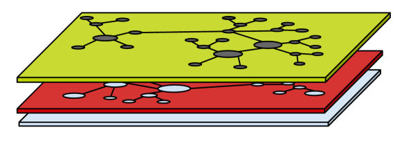
Figure 1: Multiple social network structure that shapes the social space in our simulation models.

We study the notion of context permeability in different simulation models in which agents interact using a simple consensus game. The society of agents has to adopt a binary opinion value according to a majority rule. We use the speed of consensus as a measure for self-organisation and explore the relationship between different network topologies and this measure.

We partitioned the design space of our experiments using different simulation models. Each model is designed to analyse different aspects of context permeability. In a first model [29, 30], we study the notion of permeability by overlapping social networks. In a second model [12], we analyse the dynamics introduced by switching between social contexts(neighbourhoods in different networks). This adds a temporal component that changes the dynamics of the game: agents can only perform encounters with neighbours that are active in their current context. (It also adds the chance for some agents to be isolated during the simulation.)

3.1 Simulation and Consensus Game

Our agent-based models are designed as discrete-event models. On each simulation cycle, every agent executes a simulation step. The agents are selected in a random uniform fashion for execution. This is common practice in agent-based simulation and guarantees that there is no bias caused by the order in which the agents are executed. For each simulation model, we present a description of the individual agent behaviour. Every model we present can be seen as a binary opinion dynamics model, or a consensus game. In this game, the society of agents tries to reach an arbitrary global consensus about two possible choices or opinion values. During a simulation run, each agent keeps track of the number of each opinion value of their interaction partners. In each iteration, each agent selects an available neighbour to interact with and observes its current opinion value. The agent decides to switch its current opinion choice if the observed opinion value becomes the majority of the two possible choices. The goal of the game is to reach a global consensus, but the particular choice that gets collectively selected is irrelevant. What is important is that overall agreement is achieved. In the consensus game we consider, each agent uses the previously presented external majority (EM) rule to update its opinion value (see definition 1 in section 2).

The reason we are not interested in which exact option gets selected is the same reason why we chose such a content-neutral game for the individual interactions. From the very beginning, our research questions were focused on the collective properties, the structure of the networks involved, and the dynamical outcomes of the simulations: thus leaving out issues related with individual motivations and desired results (either for any individual agent or the society). Granted, most applications of this research will often include such goals, for inquisition into complex social issues, including possibly policy design, in which the individual rationality must be considered, and will have a very strong influence on the collective outcomes.

3.2 Context Permeability

The first model of context permeability [29, 30] is designed to study the setting where an agent is immersed in a complex social world: where it engages in a multitude of relations with other agents. In this model, we consider that the context permeability is created by agents that can belong simultaneously to several relations. As an example, two agents can be simultaneously family and co-workers. While some links might not connect two agents directly, others can contain neighbourhoods in which they are related (either directly or through a common neighbour). Model 1 describes the behaviour of each agent for each simulated step.

Model 1 Context Permeability

  $M$ {Simulation Model / Environment}

  $A$ {Current Agent in Execution}

  {Randomly select a network}

  $r$ $\leftarrow$ randomUniform(0,$M.networks.length()$)

  network $\leftarrow$ $M.networks[r]$

  

  {Randomly select a neighbour}

  neighbours $\leftarrow$ network.neighboursOf($A$)

  $r$ $\leftarrow$ randomUniform(0,neighbours.length())

  partner $\leftarrow$ neighbours[r]

  

  {Update opinion and memory}

  {opinions take the values {0,1}–so they can be used as an index}

  A.memory[partner.opinion]++

  if (A.memory[partner.opinion] $>$ A.memory[A.opinion]) then

        A.opinion $\leftarrow$ partner.opinion

  end if

In this model, on each time step, each agent select a random neighbour from any social network available and updates its opinion based on the opinion of the selected partner using the external majority rule.

3.3 Context Switching

In the context switching model [12], agents are embedded in multiple relations represented as static social networks and they switch contexts with a probability $\zeta_{C_{i}}$ associated with context $C_{i}$. The switching probability is the same for every agent in a given network. Each agent switches from its current neighbourhood to another network. The agents are only active in one context at a time, and can only perform encounters with neighbours in the same context. We can think of context switching as a temporary deployment in another place, such as what happens with temporary immigration. The network topology is static; when an agent switches from one network to another, they become inactive in one network and active in their destination.

Model 2 Context Switching

  $M$ {Simulation Model / Environment}

  $A$ {Current Agent in Execution}

  {Get the current network (context is a network index)}

  cNetwork $\leftarrow$ M.networks[A.context]

  

  {Get the neighbours for the current network}

  neighbours $\leftarrow$ cNetwork.neighboursOf($A$)

  {filter by agents active in the same network}

  neighbours $\leftarrow$ {n $|$ n $\in$ neighbours $\wedge$ (n.context = A.context)}

  

  {Randomly select a neighbour}

  $r$ $\leftarrow$ randomUniform(0,neighbours.length())

  partner $\leftarrow$ neighbours[r]

  

  {Update opinion and memory}

  {opinions take the values {0,1}–so they can be used as an index}

  A.memory[partner.opinion]++

  if (A.memory[partner.opinion] $>$ A.memory[A.opinion]) then

        A.opinion $\leftarrow$ partner.opinion

  end if

  

  {Switch to another network}

  switchingProb $\leftarrow$ M.params.switchingProb(A.context)

  $r\leftarrow$ randomUniform(0,1)

  if ($r<$ switchingProb) then

        numNets $\leftarrow$ M.networks.length()

        nextNetworks $\leftarrow$ {i $|$ (i $\in$ [0,numNets[) $\wedge$ (M.networks[i] != A.context)}

        $r$ $\leftarrow$ randomUniform(0,nextNetworks.length())

        A.context $\leftarrow$ nextNetworks[r]

  end if

In this model, agents select an (active) partner from their current neighbourhood. If a partner is available, the agents update their opinion value based on EM. At the end of the interaction, the agent switches from the current context to a different one with a probability associated with its current context.

This model describes an abstract way to represent the time spent on each network using the switching probability $\zeta_{C_{i}}$. Here, the permeability between contexts is achieved using this temporal component. Context switching introduces a notion that has not been explored in the literature so far: the fact that, although some social contexts can be relatively stable, our social peers are not always available for interaction and spend different amounts of time in distinct social contexts.

4 Experimental Setup

In this section, we present all the tools and processes necessary to produce the current research output. The experiments were developed using the MASON [31] simulation framework written in Java. All the code for the simulation models can be found here [32]. Moreover, all the results presented in this article were made reproducible by using the statistical computing language R [33] and the R package knitr [34]. Knitr is used for generating reports that contain the code, the results of its execution (plots and tables), and the textual description for such results. All the R code used to produce the data analysis and the configuration files used to reproduce the data can be found in [35].

For each configuration in our experiments, we performed 100 independent simulation runs. The results are analysed in terms of value distribution, average and standard deviation, or variance over the 100 runs. Like we described in section 3.1, our models are discrete-event models. In each cycle agents execute a step in a random order: this is so that this dynamical system –our simulation model– is not influenced by the order in which agents are executed. Simulations end when total consensus is achieved or 2000 steps have passed.

4.1 Social Network Models

The social networks used in our models are k-regular and scale-free. A k-regular network is a network where all the nodes have the same number of connections. These networks are constructed by arranging the nodes in a ring and connecting each node to their next $k$ neighbours. Each network has $2k$ edges per vertex.

Scale-free networks are networks in which the degree distribution follows a power law, at least asymptotically. That is, the fraction $P(k)$ of nodes in the network having $k$ connections to other nodes goes for large values of $k$ as: $P(k)\sim k^{-\gamma}$ where $\gamma$ is a parameter whose value is typically in the range $2<\gamma<3$.

We use the method proposed in [24] by Barabási and Albert to construct the scale-free network instances using a preferential attachment. This model builds upon the perception of a common property of many large networks: a scale-free-power-law distribution of node connectivity. This feature was found to be a consequence of two generic mechanisms: networks expand continuously by the addition of new vertices, and new vertices attach preferentially to sites that are already well connected (more commonly known as “preferential attachment”). In these networks, the probability $P(k)$ of two nodes being connected to each other decays as a power law, following $P(k)\sim k^{-\gamma}$.

The network instances were generated using the b-have network library [36]. This is a Java library that allows the creation and manipulation of network/graph data structures. It also includes the more commonly used random network models from the literature.

4.2 Measuring Network Properties

We measure two structural properties of our networks: the average path length and the clustering coefficient. The average path length measures the typical separation between two vertices in the graph. The clustering coefficient measures the average cliquishness of the graph neighbourhood. This measure quantifies how close the neighbours of a node are to forming a clique. Duncan J. Watts and Steven Strogatz [25] introduced the measure to characterise a class of complex networks called small-world networks.

These properties characterise structures that can be found in the real scenarios. The small-world networks generated by the models of Watts and Strogatz for instance, model real-world social networks with short average path length, local clustering structures, and triadic closures between the nodes [25]. One shortcoming of this model, is the fact that these networks do not possess node hubs found in many real-world social networks. (Nevertheless, these models are designed to create networks with specific properties, not as general models for all kinds of real social networks)

Since we construct scenarios where we overlap highly clustered k-regular networks and scale-free networks with node hubs, we are interested in the kind of properties that emerge from merging these structures – and if/how they are comparable to the existing models –. The networks were produced by the b-have network library [36], exported to files, and analysed using the igraph R package [37].

5 Results and Discussion

In this section, we analyse and discuss the results for different experiments with both the context permeability and context switching models. We start by analysing the structural properties that arise from combining different networks. We then observe the impact of different model configurations in the convergence to consensus. We correlate the outcomes of our context permeability model simulations with the structural properties of the multi-network structures. We also explore how the new dynamics introduced by the context switching mechanism affects the consensus building process.

5.1 Overlapping Network Properties

In this first analysis, we investigate the properties of different network topologies used in our models. One of the parameters in some experiments is the number of networks in which the agents interact. Adding more networks implies the addition of more connections. We show that what is important is not just the the number of connections, but the properties of the resulting structure (when we merge the networks). We analyse the networks as follows.

Each network is generated in such a way that the node indexes are randomised. This means that we can have multiple networks with the same topology and each node can have different neighbourhoods in different networks. Also, neighbourhoods do not necessarily overlap due to the node shuffling. Adding more networks to the social space is not the same as creating a single network with twice the number of connections.

Consider figure 2. We created two random k-regular networks with k=10 and merged them ignoring edges from common neighbours. (In the simulation models this edge agglutination is not performed, we use it here for the purposes of network analysis.) Common edges are highlighted with a different colour.

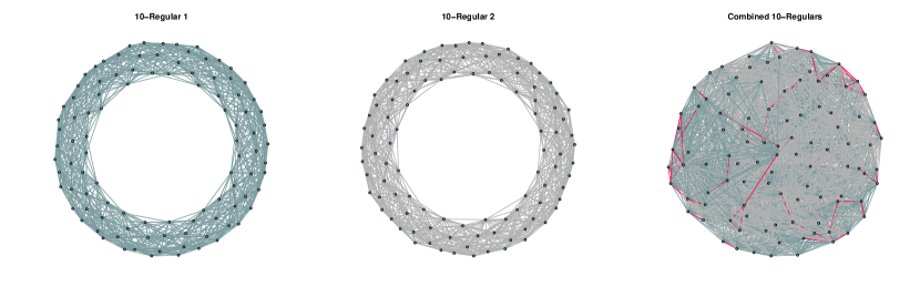
Figure 2: Overlapping of two k-regular networks, each with k=10.

Table 1: Properties for overlapping of two k-regular networks, each with k=10.

	Nodes	Edges	Clustering Coef.	Avg. Path Length
10-regular 1	100	1,000	0.711	2.980
10-regular 2	100	1,000	0.711	2.980
Combined	100	1,790	0.512	1.638
20-regular	100	2,000	0.731	1.788

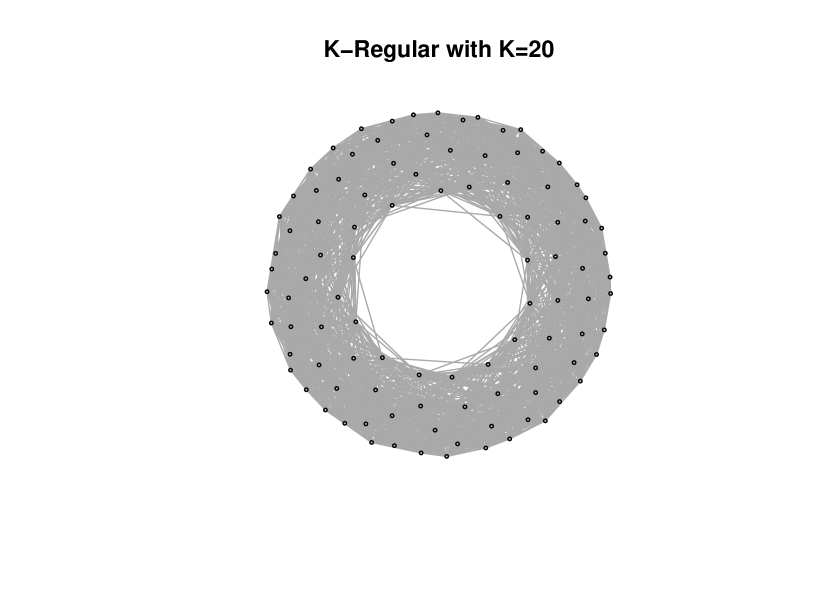
Figure 3: Single k-regular network with k=20.

The networks are drawn using the Kamada-Kawai Layout [38] which treats the “geometric” (Euclidean) distance between two vertices in the drawing as the “graph theoretic” distance between them in the corresponding graph. We can see by the results of the layout in figure 2, that the distance between nodes in the network has decreased, this is also confirmed by the reduced average path length of the combined networks (see table 1). To illustrate our point, we analysed one k-regular network with k = 20 (see figure 3 and the corresponding entry on table 1). The clustering coefficient of a 20-regular network is approximately the same as the one of a 10-regular network (higher than the combination of two 10-regular networks). The average path length also decreases as there are more connections between previously distant nodes. As we will show, these properties may vary due to the node indexes being subjected to random permutations.

Since we model the agent social space as a multitude of networks, we need to investigate the properties resulting from the merging of these networks. We do this empirically by taking the network instances used in the simulations, and analysing the distribution of clustering coefficient and average path length for the different configurations.

5.1.1 Properties of Overlapping K-Regular Networks

We will now investigate what kind of properties we can get from merging k-regular networks. First, we analysed the distribution for the average path length and the clustering coefficient values over 100 network instances (each with 100 nodes). From a box plot preliminary analysis (see figures A.2 and A.1), we can see that the average path length does not vary much for the 100 instances, as such, the average makes a good descriptor for these properties.

Figure 4 shows the average value for the average path length of 100 k-regular network instances (each with 100 nodes). We can see that the average path length changes more drastically when we go from 1 to 2 networks. This is precisely the effect we can see in figure 2. Merging these networks at random effectively creates multiple shortcuts between points that were not connected in the original k-regular topology. Beyond this point, adding more networks does not modify this structural property in a significant way. Note that, since each network has 100 nodes, with $k=50$ the network is fully connected (hence the average path length being 1).

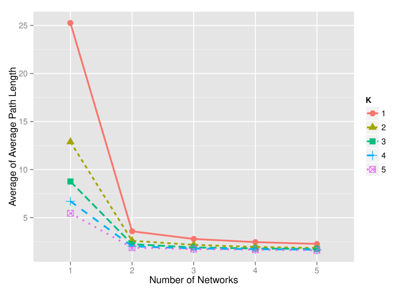
(a)

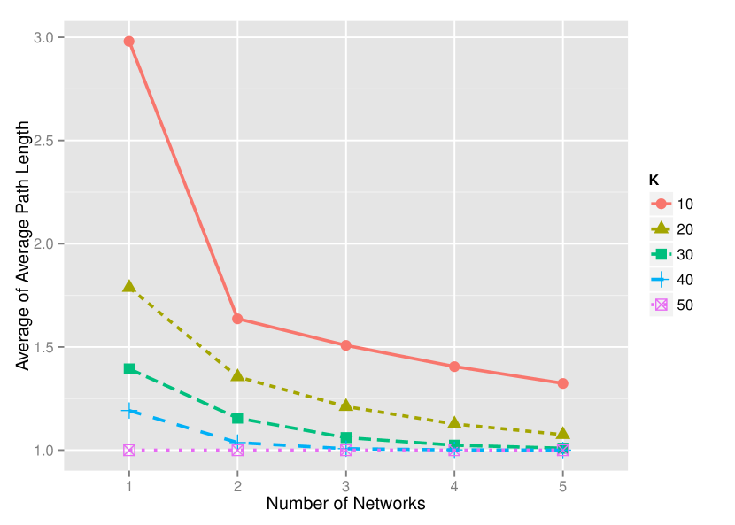
(b)

Figure 4: Average value for the average path length of 100 instances of overlapping k-regular networks (containing 100 nodes each) with k={1,2,3,4,5} (4(a)), and k=  {10,20,30,40,50} (4(b)).

Figure 5 shows the results for the average clustering coefficient of 100 instances of overlapping k-regular networks. Adding multiple networks changes the clustering coefficient of the resulting structure. For $k\leq 20$, the clustering coefficient drops when we add a second network. This happens because when we merge these networks, their connectivity is not high enough to generate shortcuts with tightly clustered neighbourhoods. The clustering coefficient is computed by taking the average local clustering coefficient of each node in the network. An initial highly clustered k-regular network (with all the nodes having the same structure) is affected when you modify the node neighbourhoods in such a way that some are more clustered than others. Networks with $k=1$ have a ring-like structure, so there are no nodes forming a clique with their neighbours.

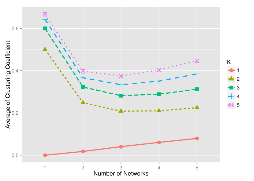
(a)

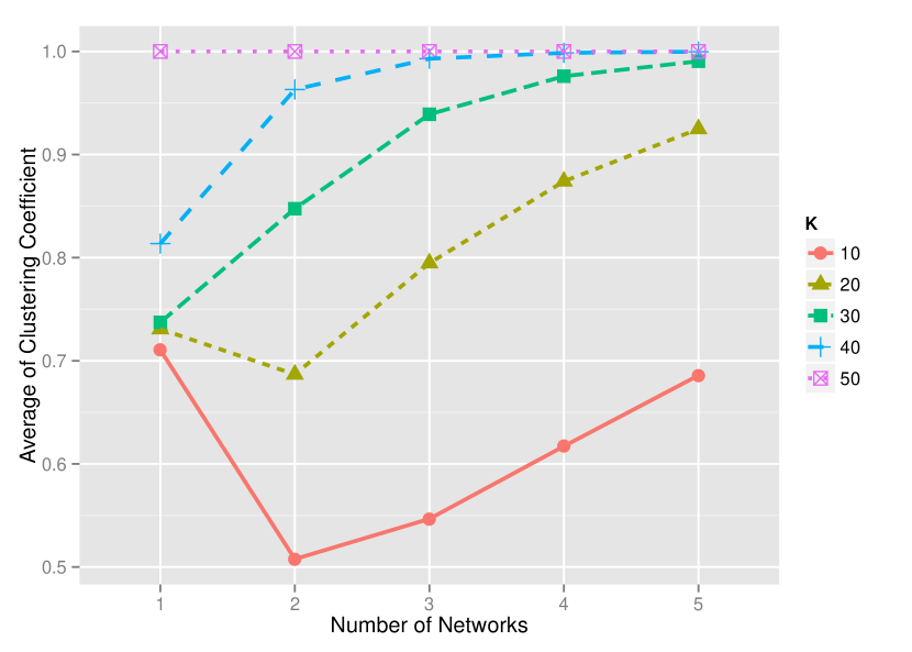
(b)

Figure 5: Average value for the clustering coefficient of 100 instances of overlapping k-regular networks (containing 100 nodes each) with  k={1,2,3,4,5} (5(a)), and k = {10,20,30,40,50} (5(b)).

5.1.2 Properties of Overlapping Scale-free Networks

We also looked at the properties that result from merging scale-free networks (see figure A.3). Like the previous results, the properties don’t vary much between the 100 different instances. We can then say that specific configurations display a specific average path length and clustering coefficient both for k-regular networks and scale-free networks. We plotted the average of the average path length (figure 6(a)) and clustering coefficient (figure 3(b)) for each overlapping network configuration.

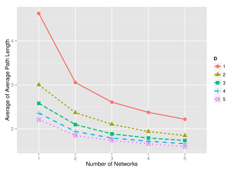
(a)

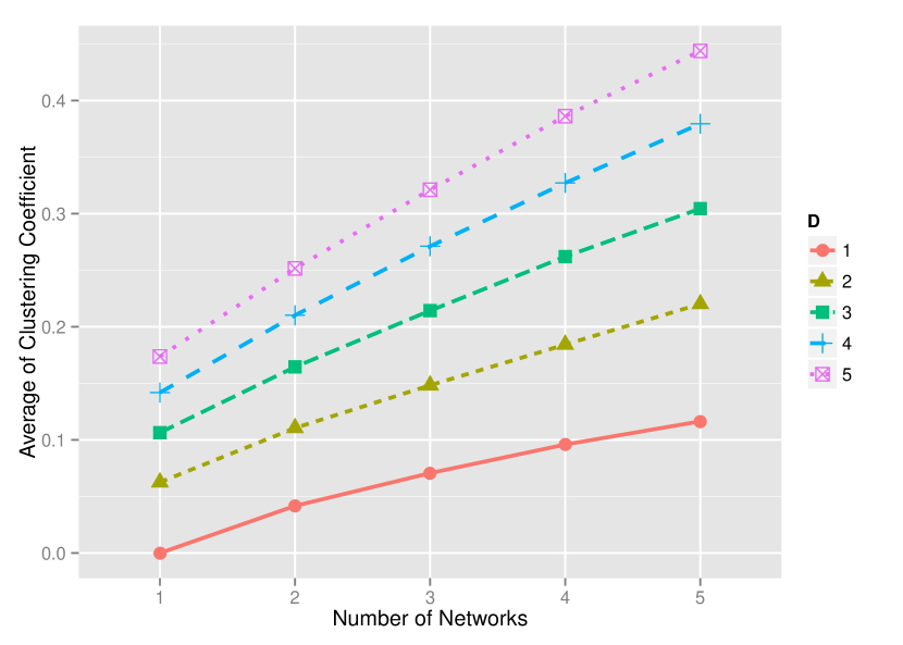
(b)

Figure 6: Average value for the average path length (3(a)) and clustering coefficient (3(b)) for 100 instances of overlapping scale-free networks (containing 100 nodes each).

The parameter $d$ (figure 6) dictates how many edges are added by preferential attachment (see section4.1). For $d=1$, the resulting network is a forest: a network composed of disjoint tree graphs. Figure 6(a) shows us that the average path length still decreases consistently when we add more networks. One of the characteristics of scale-free networks is its short average path length, thus, for $d\geq 2$, adding more edges does not make a significant difference. Scale-free networks also have a reduced clustering coefficient (see figure 6(b)). When we add more networks the clustering coefficient increases.

5.1.3 Merging K-Regular with Scale-Free Networks

Finally, we look at what happens when we merge k-regular networks with scale-free networks. We didn’t make an exhaustive analysis for this configuration, but we show what is the resulting structure of such merging. You can see in figure 7 that this results in a network with a lower average path length due to the shortcuts created by the scale-free network. It is also less dense than the structure with two 10-regular networks (figure 2). We consider only the merging of two networks.

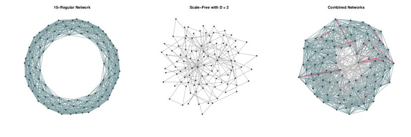
Figure 7: Overlapping of a 10-regular with a scale-free network with D=2.

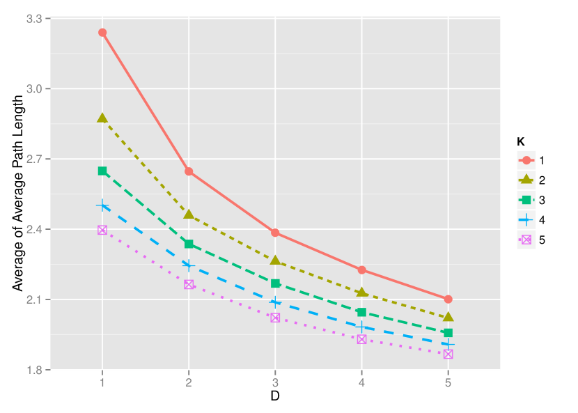
(a)

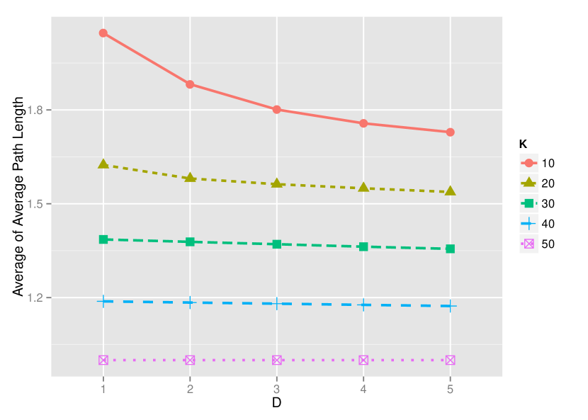
(b)

Figure 8: Average average path length for 100 instances of heterogeneous network configurations: one scale-free with $d=\{1,2,3,4,5\}$ and one k-regular network with $k=\{1,2,3,4,5\}$ (8(a)) and $k=\{10,20,30,40,50\}$ (8(b)). (See the respective box plots in the appendix: figure A.4).

Figure 8 shows the average path length of 100 independently generated instances of combinations of one k-regular network and one scale-free network with different values $k$ and $d$ respectively. For configurations where the k-regular networks have low values of $k$ (figure 8(a)), adding a scale-free network always decreases the average path length. Moreover, the higher the $d$, the lower the path length (as more connections are formed between different nodes). With higher values of $k$ (figure 8(b)) however, increasing the value of $d$ does not decrease the average path length. This is not surprising given the level of connectivity of this structure. The first network is already highly dense and connected, so adding a few extra connections doesn’t matter; what does matter is that we have a scale-free network creating shortcuts between nodes that were not previously connected.

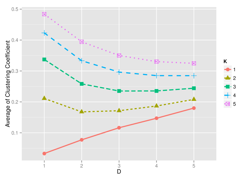
(a)

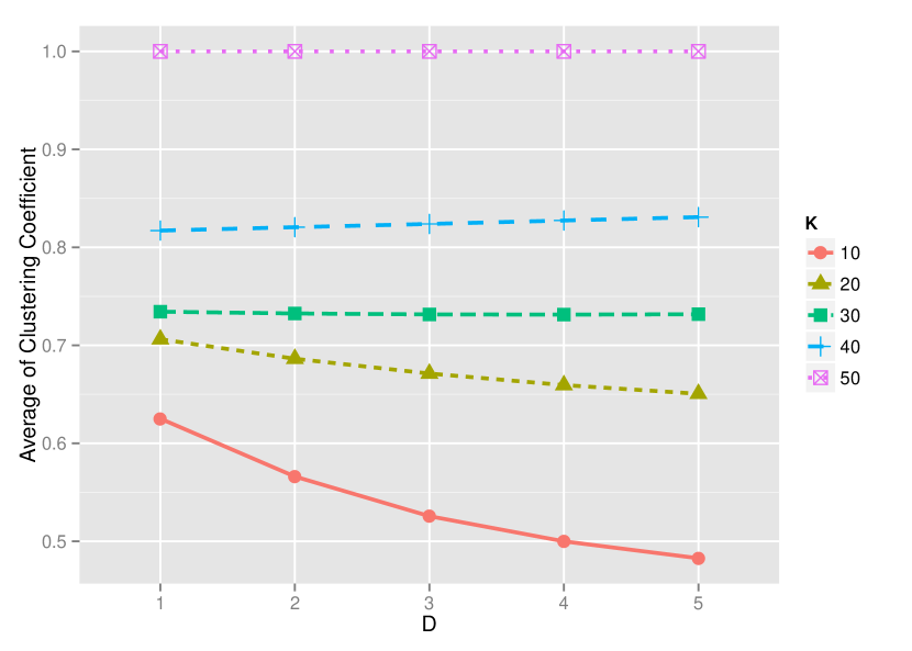
(b)

Figure 9: Average clustering coefficient for 100 instances of heterogeneous network configurations: one scale-free with $d=\{1,2,3,4,5\}$ and one k-regular network with $k=\{1,2,3,4,5\}$ (3(b)) and $k=\{10,20,30,40,50\}$ (See the respective box plots in the appending: figureA.5).

Figure 9 shows the results for the clustering coefficient. These are similar to the results we get for k-regular networks (see figure 5). The difference is that we are not adding more networks but rather increasing the parameter $d$ of the scale-free (number of connections added by preferential attachment for each note). In this case, the effects are qualitatively similar with the ones of merged k-regular network with low value of $k$. In contrast, for high values of $k$ (figure 9(b)), a higher value of $d$ is not enough to make the network more clustered. This happens because scale-free networks are more sparse and have a very low number of triangles between nodes.

5.2 Context Permeability

In this section, we discuss the results for various sets of experiments on the context permeability model [29, 30]. First, we used k-regular and scale-free networks with our model. Each network layer was configured with the same topology. We analyse the context permeability model in terms of convergence to consensus: the ratio of simulations that converged to total consensus over 3000 runs; and how many agent encounters were needed for this to happen.

5.2.1 Convergence Ratio

To analyse the ratio of convergence to consensus for different network configurations, we correlate this ratio with the properties that the combined network structure exhibits. As we have seen in section 5.1, the properties don’t vary much for different random instances, so we use the average as the descriptor for these properties.

The following tables show the results of our simulations. Table  2 shows the percentage of total consensus achieved with 2000 cycles for 3000 runs. For k-regular networks with a small $k$, consensus is rarely achieved with a single network. However, as soon as we add more networks, consensus is achieved in a significantly greater number of occasions. These results are especially interesting for the scale-free networks (table 3): as soon as we add more networks, for a scale-free with $d\geq 2$, we can achieve consensus in a lot of occasions. This is to show that achieving consensus is not just a matter of connectivity. With scale-free networks, we can achieve consensus more often with less clustered networks. This convergence is achieved not because of the clustering coefficient but rather due to lower average path length. This is difficult to visualise using only the tables and the previous plots so, to confirm this hypothesis, we measured the Spearman’s correlation between the ratio of convergences to consensus, the average average path length, and the average clustering coefficient for the corresponding network configurations (see table 4).

Table 2: Ratio of convergence to total consensus in 3000 independent runs with with a number of concomitant networks ($\#$ nets.) equal in kind: k-regular networks with $k=\{1,2,3,4,5,10,20,30,40,50\}$.

	value for k
# nets.	$1$	$2$	$3$	$4$	$5$	$10$	$20$	$30$	$40$	$50$
1	$0.0000$	$0.0000$	$0.000\,666\,7$	$0.0050$	$0.016\,33$	$0.1830$	$0.6713$	$0.9673$	$1.0000$	$1.0000$
2	$0.0770$	$0.5887$	$0.813\,666\,7$	$0.8967$	$0.934\,67$	$0.9817$	$0.9977$	$1.0000$	$1.0000$	$1.0000$
3	$0.6560$	$0.9417$	$0.978\,000\,0$	$0.9920$	$0.994\,33$	$0.9997$	$1.0000$	$1.0000$	$1.0000$	$1.0000$
4	$0.8780$	$0.9867$	$0.996\,666\,7$	$0.9993$	$1.000\,00$	$1.0000$	$1.0000$	$1.0000$	$1.0000$	$1.0000$
5	$0.9497$	$0.9937$	$0.999\,333\,3$	$1.0000$	$1.000\,00$	$1.0000$	$1.0000$	$1.0000$	$1.0000$	$1.0000$

Table 3: Ratio of convergence to total consensus in 3000 independent runs with a number of concomitant networks ($\#$ nets.) equal in kind: scale-free networks with $d=\{1,2,3,4,5\}$.

	value for d
$\#$ nets.	$1$	$2$	$3$	$4$	5
1	$0.0000$	$0.2903$	$0.8590$	$0.9573$	$0.9873$
2	$0.2840$	$0.9287$	$0.9877$	$0.9973$	$0.9980$
3	$0.7793$	$0.9850$	$0.9970$	$1.0000$	$1.0000$
4	$0.9287$	$0.9977$	$0.9997$	$1.0000$	$1.0000$
5	$0.9737$	$0.9997$	$1.0000$	$1.0000$	$1.0000$

Table 4: Spearman’s correlation between convergence ratio (CR), average average path length (APL) and clustering coefficient (CC) along with the respective p-value and confidence interval, for a confidence level of 95%.

network model	X	Y	Correlation	CI(95%)	p-value
k-regular	CR	APL	-0.726	[-0.836, -0.561]	$2.437\text{\times}{10}^{-09}$
k-regular	CR	CC	0.264	[-0.015, 0.505]	$0.064$
scale-free	CR	APL	-0.912	[-0.961, -0.808]	$2.28\text{\times}{10}^{-10}$
scale-free	CR	CC	0.633	[0.318, 0.823]	$0.000\,677\,6$

5.2.2 Number of Encounters to Achieve Consensus

We now analyse the convergence in terms of average number of meetings during a simulation run. Since the maximum number of simulation cycles is 2000, the maximum number of encounters is 2 000 000 (we have 100 agents and each one performs one encounter per cycle). We show that for some configurations, the average of encounters is not a good descriptor since it varies greatly from run to run. Rather than considering the average, it is better to look at the distributions of these measures. Nevertheless, we included the data with all the average number of encounters, as well as the respective standard deviations for different network configurations. You can find this data in appendix B.

First, we present the results for k-regular networks. To observe the distribution of the number of encounters, consider the box plots for $k=\{1,2,3,4,5\}$ (figure 10(a)) and $k=\{10,20,30,40,50\}$ (figure 10(b)). Figure 10 shows the results for configurations with a number of networks $\geq 3$ (since less networks lead to much worse results in terms of convergence speed). These plots reveal two types of situations: the typical runs, in which the number of encounters doesn’t vary much, and some “outlier runs,” which present some interesting dynamics, as we will see later on.

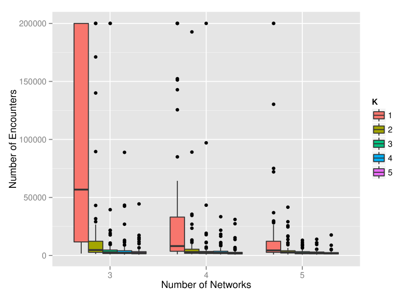
(a)

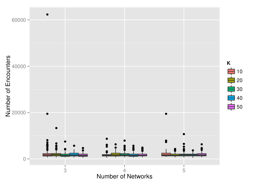
(b)

Figure 10: Number of meetings over 100 independent simulation runs for multiple k-regular networks: $k=\{1,2,3,4,5\}$ (10(a)) and $k=\{10,20,30,40,50\}$ (10(b))).

Figure 10 shows us results qualitatively similar to what we previously observed for convergence ratios (see section 5.2.1). Networks with lesser connectivity and a greater average path length lead to total convergence less often. The simulation outcomes also vary much more in comparison with the other configurations ($k>1$ and $networks\geq 3$).

Notice that for $k=3$ and $networks=3$ (10(b)), we still have runs that deviate from what we consider the typical behaviour. Instead of disregarding this as an outlier, we explore this behaviour to better understand the dynamics of our External Majority consensus game.

We analysed the network structure from this run and observed that there were no distinct differences between the network instances from the “outlier run” and the ones of the “typical” run. This pointed to the consensus game itself as a possible cause for the irregular behaviour – not to the network structure –. What happens is that the agents reach a state from which converging towards consensus is significantly harder. Villatoro [39] found that some complex network models lead consensus games to form metastable sub-conventions. These are very difficult to break and reaching 100% agreement is not as straightforward as assumed by previous researchers. We are not concerned with this difficulty, instead, we want to explore how to describe what happens in similar cases. Figure 11 shows the consensus progression for two simulation runs a typical case and the outlier.

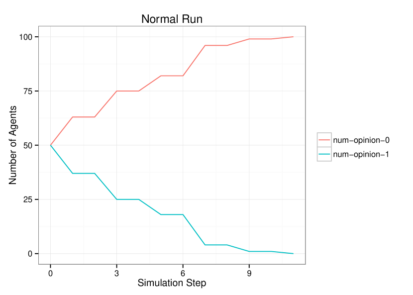
(a) Typical Run

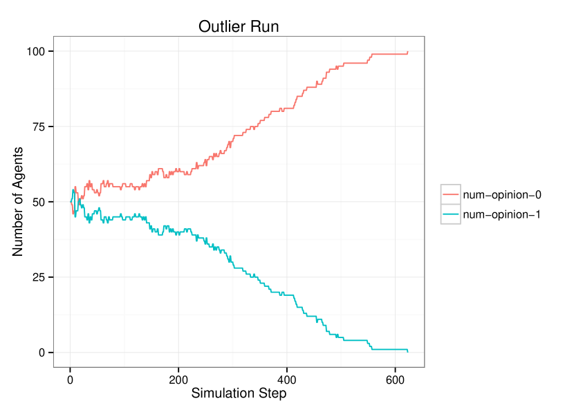
(b) Outlier Run

Figure 11: Number of agents with each opinion during a simulation run: typical run in 11(a) and “outlier run” in 11(b).

We take the outlier in the configuration with $k=3$ and $networks=3$, and look at the memory that agents use in the consensus game. As we described previously, agents record the number of individuals encountered with each opinion value (two possible values in this case). We look at the average difference between the number of values observed for all the agents. We also look at the variance to find how the opinion observations evolve throughout the simulation. Figure 12 shows the average difference between opinion memory for the first 10 steps (which was when the simulation converged for the normal run).

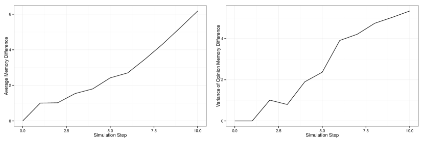
(a) Typical Run

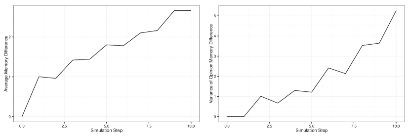
(b) Outlier Run

Figure 12: Average and variance of the difference between opinions observed for the 100 agents: typical run in figure 12(a) and first steps of the“outlier run” in figure 12(b).

We can see that both the average difference in the opinion memory and the variance grow faster in the normal run than in the outlier run. This is not enough to establish a significant difference between the two. Moreover, the memory differences are quite similar, but the number of agents for each opinion was quite even. This happens due to the position of agents in the network and their initial opinion values. These circumstances led the agents to a initial stability. Note that the opinion difference continues to rise throughout the simulation along with the variance. The variance starts to increase more rapidly after 200 steps. The exponential growth reveals that the convergence to consensus is not done evenly throughout the network, this is one of the reasons why consensus takes more time to be achieved. Also, the low variance in the first $200$ steps shows us that the opinion strength was evenly distributed: we have almost the same number of agents for each opinion but the memory differences are qualitatively the same for both opinions. As soon as this variance increases, one of the opinions breaks the stable state and convergence towards global consensus begins.

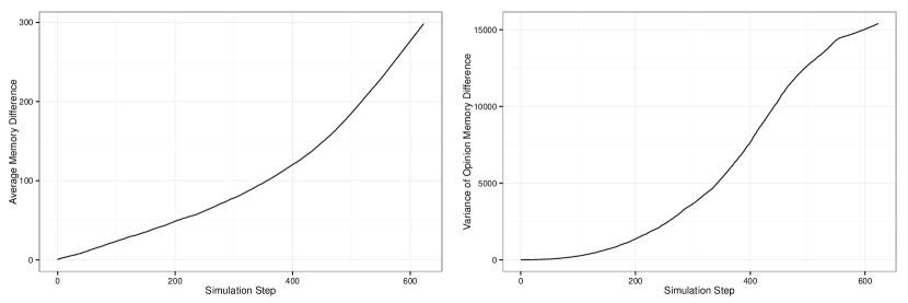
Figure 13: Average and variance of the difference between opinions observed for the 100 agents throughout the outlier run.

In other words, different neighbourhoods in the network lead to different opinion observation configurations (possibly even creating self-reinforcing structures). Thus, the influence of heterogeneous connectivity is reflected on the growth of opinion difference variance.

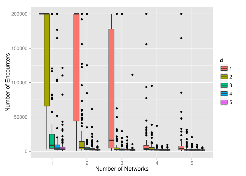
(a)

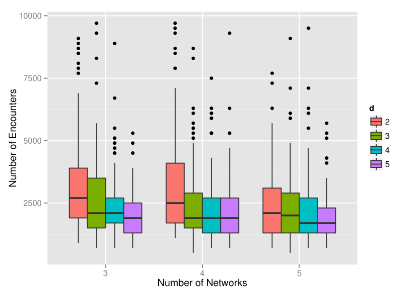
(b)

Figure 14: Number of meetings over 100 independent simulation runs for multiple scale-free networks: with d={1,2,3,4,5} (14(a)) with a zoom on the best configurations in 14(b).

Figure 14 shows the average number of encounters during 100 independent simulation runs for scale-free networks. (We don’t include the configuration for one network and $d=1$ because these never converge.) The convergence ratio is very low for the configurations with one network $d=2$ and 2 networks with $d=1$; hence the high number of encounters (see also table 3).

These results are similar to those of k-regular in that adding more networks speeds up the convergence to consensus. The difference is that more “atypical” runs occur with multiple scale-free networks. Again, this is the effect of these types of topologies. As we discussed previously, in these less connected topologies, agents are more prone to be arranged in such a way that progression towards consensus is more difficult to attain due to bottlenecks. Different regions in the network might converge towards different opinion values.

5.2.3 Heterogeneous Network Configuration

We also performed experiments with mixed network topologies: we used one scale-free and one k-regular networks. Table 5 shows the convergence ratio for the heterogeneous network configuration with the multiple values for $d$ and $k$ for the scale-free and k-regular respectively.

Table 5: Ratio of convergence to total consensus in 3000 independent runs with two networks: one k-regular and one scale-free network with different $k$ and $d$ values respectively.

	k
d	$1$	$2$	$3$	$4$	$5$	$10$	$20$	$30$	$40$	50
1	$0.18$	$0.47$	$0.55$	$0.67$	$0.61$	$0.76$	$0.77$	$0.81$	$0.75$	$0.82$
2	$0.63$	$0.72$	$0.88$	$0.89$	$0.90$	$0.97$	$1.00$	$1.00$	$0.99$	$1.00$
3	$0.77$	$0.86$	$0.87$	$0.97$	$0.98$	$0.99$	$0.98$	$0.99$	$1.00$	$1.00$
4	$0.73$	$0.92$	$0.92$	$0.97$	$0.96$	$0.96$	$0.99$	$1.00$	$1.00$	$1.00$
5	$0.87$	$0.85$	$0.94$	$0.94$	$0.98$	$0.99$	$1.00$	$1.00$	$1.00$	$1.00$

One of the differences between this configuration and the previous ones can be observed in the simulations with $d=1$ and $k=1$. The convergence ratio is higher than with $2$ $1-regular$ networks (see table 2) – but not better than two scale-free networks. This happens because with $k=1$ the network is basically a ring and has the maximum possible average path length for a connected graph. Adding two rings improves the convergence ratio but the underlying structure is still very susceptible to self-reinforcing structures (a connected sub-graph is basically a line). Adding a scale-free changes this drastically as we are mixing tree-like network components with a ring.

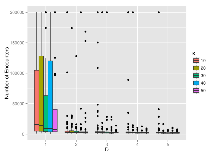
(a)

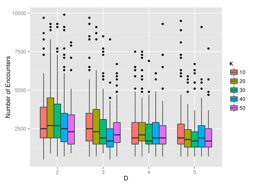
(b)

Figure 15: Number of meetings over 100 independent simulation runs for heterogeneous configuration: one k-regular network with $k=\{1,2,3,4,5\}$ and one scale-free network with $d\{1,2,3,4,5\}$. Figure 15(b) shows a zoom on the best configurations.

Figure 15 shows the results for the number of encounters necessary for the agents to achieve consensus. We focus on the k-regular networks with higher values of $k$. We can see that with these two networks, the configurations with values of $d>=2$ for scale-free networks produce drastically better results in terms of speed of convergence. The data for the average number of encounters, as well as the respective standard deviations referent to the results in figure 15, can be found in appendix B, table B.3.

5.3 Context Switching

In this section, we present the results relative to the context switching model. The difference between this model and the previous one is that the agents no longer interact in multiple networks at the same time (being able to select any neighbour at a given simulation step). In this model, they become active in a single network at a time. Agents can switch to a different network at the end of each step. The switching mechanism uses a probability associated with each network. With this new idea of swapping contexts, we covered some space left undeveloped in Antunes and colleagues original work [29, 30].

As we discussed in section 3.3 (see model 2), the switching probability dictates the frequency with which an agent switches from the current network after an encounter has been performed. In an abstract manner, this allows us to model how much time agents spend on each network. A further development of this model will be to assign different preferences to different networks for each agent. This can help us model phenomena such as real-world agents that dedicate more or less time consuming content from different social networks. For now, we attribute this probability to the network to restrain the model complexity.

5.3.1 Exploring the Switching Probability

We first look at the influence of the new parameter (switching probability) in the convergence to consensus. We span the switching probability between $0$ and $1$ in intervals of $0.05$. We do this for 2 networks with k-regular and scale-free topologies. Figure 16 shows the results for two k-regular networks: one configuration with $k=10$ and one configuration with $k=30$. We use these two configurations to study the relationship between the number of encounters, the switching probability parameter, and the connectivity of the networks. Remember that with $k=30$ the average path length is also lower (section 5.1.1).

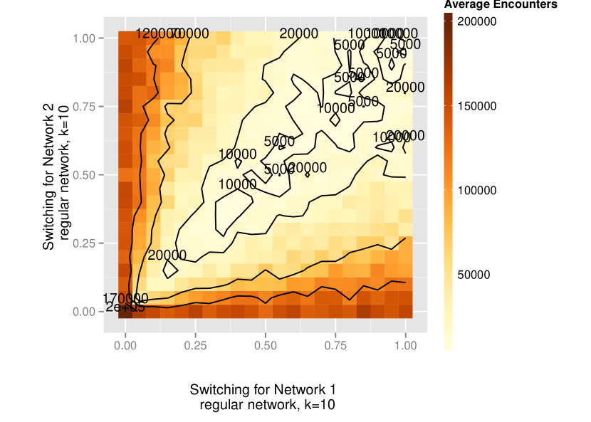
(a) 10-regular Networks

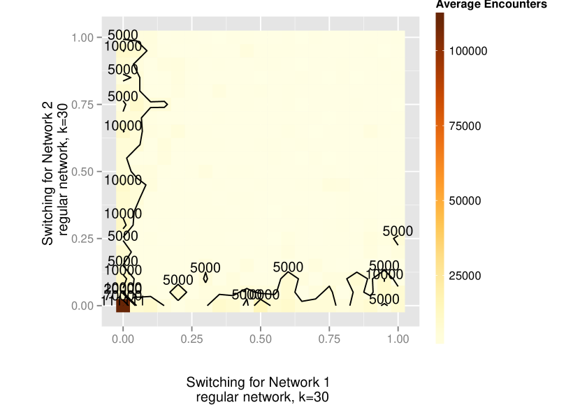
(b) 30-regular Networks

Figure 16: Contour plot for the average number of meets during a simulation for 100 independent runs: 2 10-regular networks (16(a)) and 30-regular networks (16(b)). See the perspective plots in appendix C.

For smaller values of $k$, symmetry in the context switching probability (having the same probability in both networks) is more important if the agent switches less from one of the networks. Switching less from one network means spending more time in that network. This means that switching more from the other network can be disruptive to a neighbourhood that has already converged to a sub-convention. This can be observed in configurations with k-regular networks (figure 16(a)) but it is especially apparent in scale-free networks (figure 17(a)).

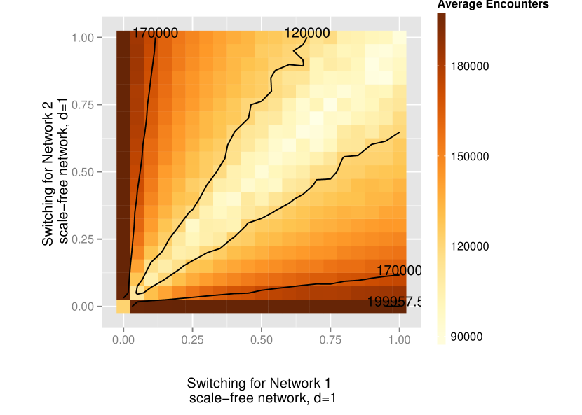
(a) Scale-Free $d=1$

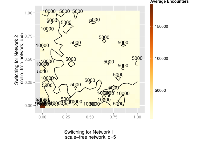
(b) Scale-Free $d=5$

Figure 17: Contour plot for the average number of meets during a simulation for 100 independent runs: 2 scale-free networks with $d=1$ (17(a)) and $d=5$ (17(b)). See the perspective plots in appendix C.

When we increase the connectivity (and lower the average path length), both in k-regular and scale-free networks, the switching probability becomes “irrelevant” –for any probability value, the speed of convergence will be the same–. The exception is obviously when considering the switching probability with value $0$. In this case, agents are isolated (they are initially equally distributed throughout the networks) and reaching consensus becomes very hard. (Especially because agents are active only in one network and this can create disconnected graphs.)

One major difference from the previous model is that the agents no longer interact with a neighbour from any network at any time. The neighbour selection has to be made from the network they are currently active in. This causes the agents to spend different amounts of time in different networks. An agent can be very influential in one network – being a very central node in that context – and marginally important in another: in a sense its opinion in one network can be more important to overall convergence than in other network, due to its position in the network.

To explore the contribution of connectivity to the new context switching dynamics, we setup two scale-free networks; one with $d=1$ and the other with $d=5$. We then spanned the switching probability in increments of $0.05$. The results can be seen in figure 18.

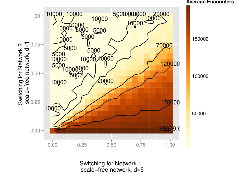
Figure 18: Contour plot for the average number of meets during a simulation for 100 independent runs: 2 scale-free networks, the first with $d=5$ and the second with $d=1$. See the perspective plots in appendix C (figure C.5).

In this case it is more important (to convergence speed) to switch from the network with lower average path length and a forest-like composition (and a probability of at least the same value or more than the one of the other network with $d=5$). The same can be observed when we mix k-regular with scale-free networks (see figure 19).

Switching less from the less connected network is bad in both cases: it is possible that spending more time in the network with bigger neighbourhoods allows for a stabler convergence. Sub-conventions can emerge in scale-free networks with $d=1$ because usually some network regions are isolated by a single node – the root of the sub-tree they belong to.

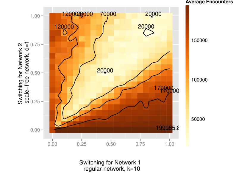
Figure 19: Contour plot for the average number of meets during a simulation for 100 independent runs: one 10-regular network (k=10) and a scale-free network with $d=1$. See the perspective plots in appendix C (figure C.6).

5.3.2 Comparison with Context Permeability

Finally, to compare the context switching model with the previous model of context permeability, we froze the switching probabilities with values $\zeta={0.25,0.5,0.75}$ and varied the number of networks. (We considered these values because they conveniently characterise the probability in low, medium and high switching.) We compare the results with the context permeability in terms of average number of encounters to achieve consensus. Note that in some cases, due to the distribution of the number of encounters, the average is not an accurate descriptor for the convergence. Nonetheless, configurations with highly variable outcomes usually produce an average that is qualitatively distinct from the rest (see figure 10 in section 5.2.2). We took the average number of encounters during the simulations to compare the context switching model with the context permeability model.

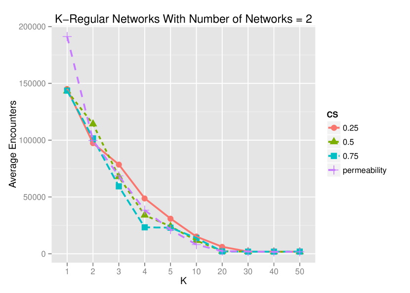
(a)

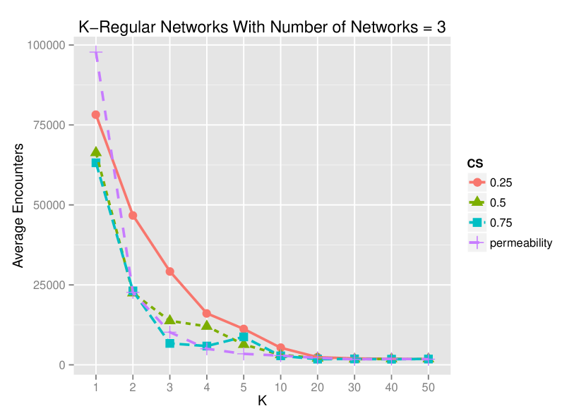
(b)

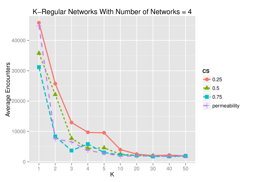
(c)

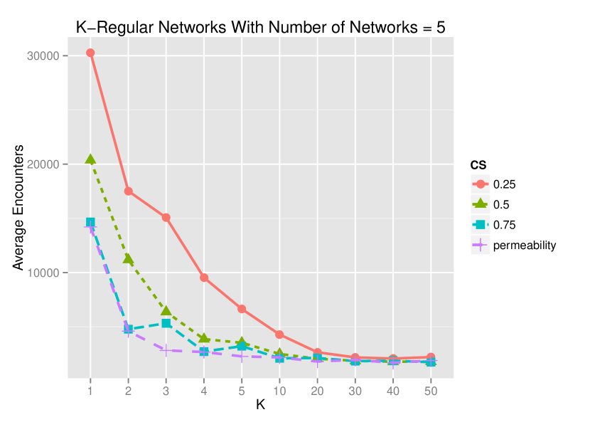
(d)

Figure 20: Average number of encounters during a simulation for 100 independent runs with k-regular topologies in all the network layers. We compare the results of context switching with context permeability with a $numberofnetworks=\{2,3,4,5\}$. The switching probability is the same in all the networks.

Figure 20 shows that for 2 networks the results in terms of number of encounters for the context switching approximate those for context permeability. When we increase the number of networks ($n\geq 3$), the configurations with higher switching probability lead the results to be closer to what happens in context permeability. This is no surprise since more switching makes agents switch more often between networks and consequently allows them too choose more often from different neighbourhoods. This is almost the same as having a larger neighbourhood to choose from, which is what happened in the context permeability model.

The surprise was that for values of $k\geq 20$, the results where practically the same for both models independently of the switching probability – even when we increased the number of networks, the number of encounters remained around $2000$ on average for all the models. Above a certain level of neighbourhood size (and overlapping, which causes the average path length to drop), the switching probability becomes less influential. It is still important that we get comparable results because we are introducing a temporal component that was never explored before in these types of opinion dynamics models: the fact that the agents can become active in different networks at different points in time.

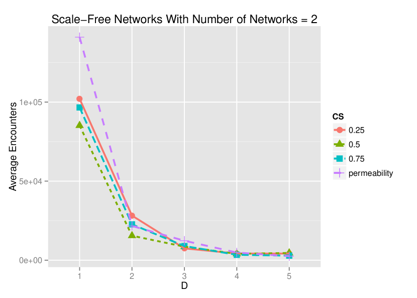
(a)

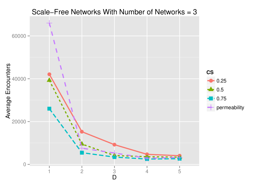
(b)

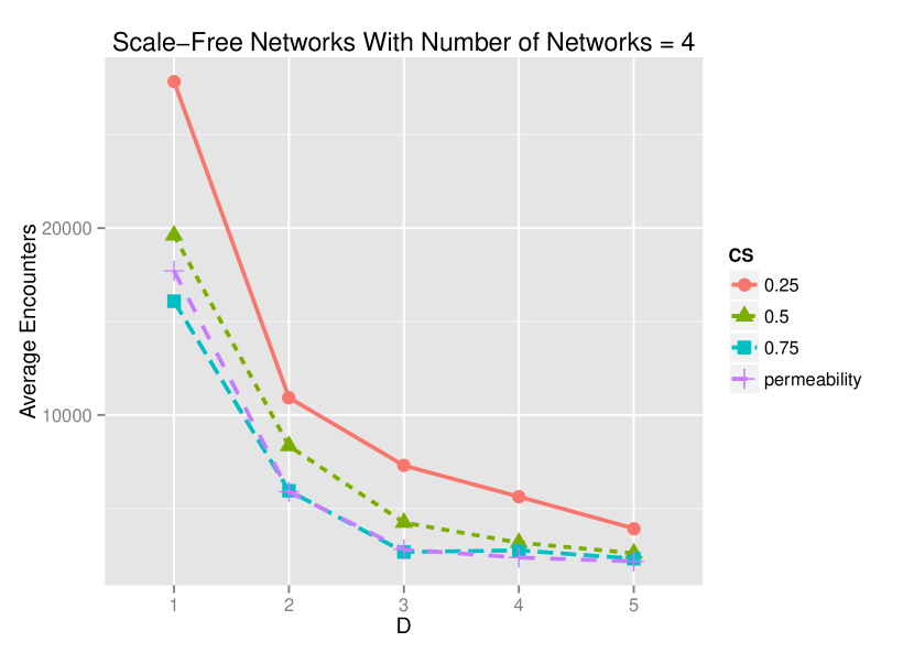
(c)

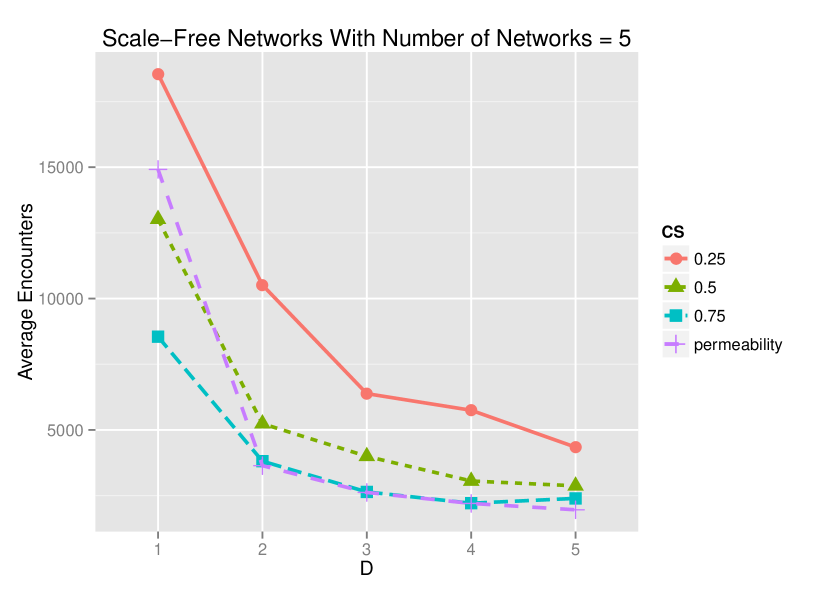
(d)

Figure 21: Average number of encounters during a simulation for 100 independent runs with scale-free topologies in all the network layers. We compare the results of context switching with context permeability with a $numberofnetworks=\{2,3,4,5\}$. The switching probability is the same in all the networks.

For scale-free networks, figure 21 shows us similar results. Switching with a higher probability displays results similar with those of context permeability. In this case, adding more networks makes so that lowering switching probabilities displays slightly worse results. This influence comes from the neighbourhoods being considerably smaller in scale-free networks – even with values of $d=5$ – so the impact of low switching was bound to be noticed.

An increasing number of networks seems to always reduce the number of encounters to achieve consensus in both models. This happens due to what we called permeability. Having multiple points of dissemination that permeate between different social networks enhances the overall convergence to consensus. With permeability there are more previously isolated nodes being reached in sparsely connected networks such as scale-free networks.

6 Conclusions

In this article, we analysed and discussed our modelling framework for multi-relational models of social spaces. These results show that not only contexts play an important role in the dissemination of consensus in artificial agent societies, but also that simple mechanisms can generate a great deal of complexity (especially in those scenarios where conventions are being co-learned by multiple agents). Adding more networks to our opinion dynamics model leads to outcomes where consensus was achieved not only more often but also faster. In particular, our results show that achieving convergence (i.e. total consensus in a network) is not a matter of connectivity. With scale-free networks we managed to achieve consensus more often and quicker than with less clustered networks. This conclusion is especially important for application (or models) dealing with real-world social phenomena, many times represented with such networks.

The second innovation presented in this article was the fact that our model describes an abstract way to represent the time spent on each network using the switching probability. This temporal component introduces a new dynamic to the study of opinion dynamics. Considering that in agent neighbourhoods, agents might not be available at all times – and spend different amounts of time in different neighbourhoods–, this is an important factor to be included in simulation models (either representing real-world systems with different levels of abstraction, or artificial agent societies for particular applications).

Future work includes the analysis of different complex network models. While k-regular and scale-free networks are two of the most pervasive network examples in social simulation, there has been a growing number of models with different properties inspired by real-world phenomena that can be considered. We will also analyse the networks according to different properties such as betweeness centrality of certain nodes. Moreover, we plan to apply what we learned with our consensus games to cooperation problems. Constructing agents that can learn both behaviour and coordination procedures is a difficult task (especially when working with large distributed artificial societies). Consensus games such as this one can be used to reduce the search space in problems where agents need to cooperate or coordinate in a decentralised fashion.

While the convergence and number of encounters seem to be correlated with the average path length, this might not be the only property that plays a role in faster convergence to consensus. Correlation is just an informal tool that helps us assert if some monotonic relationship exists. More research is needed to find out, for instance, if self-reinforced structures –like the ones reported by [39]– exist in our multi-network structures. In particular, we are interested in finding out if permeability mitigates the effects of such phenomenon.

We have seen that context permeability by context overlapping or switching can provide a fairly straightforward modelling methodology. This can be used to compose simulation scenarios for more complex social spaces. What remains to be done is to identify more precise contextual structures in real-world networks. While capturing the structure of real social network can be a daunting task, we do have pervasive records of networking activity between social actors: online social networks. Analysing these can lead us to insights about complex structural properties that emerge from user activity, and contexts that can be identified within those networks. A difficult –but not impossible– prospect for further research would be to track similar contexts between different real online social networks.

Appendix A Overlapping Network Properties

A.1 Homogeneous Network Topology Configurations

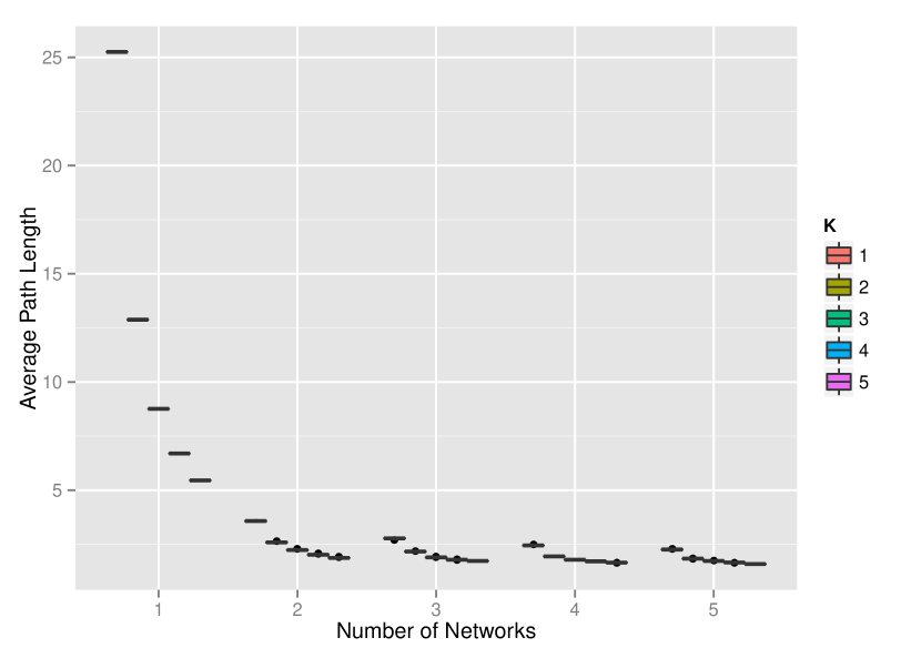
(a)

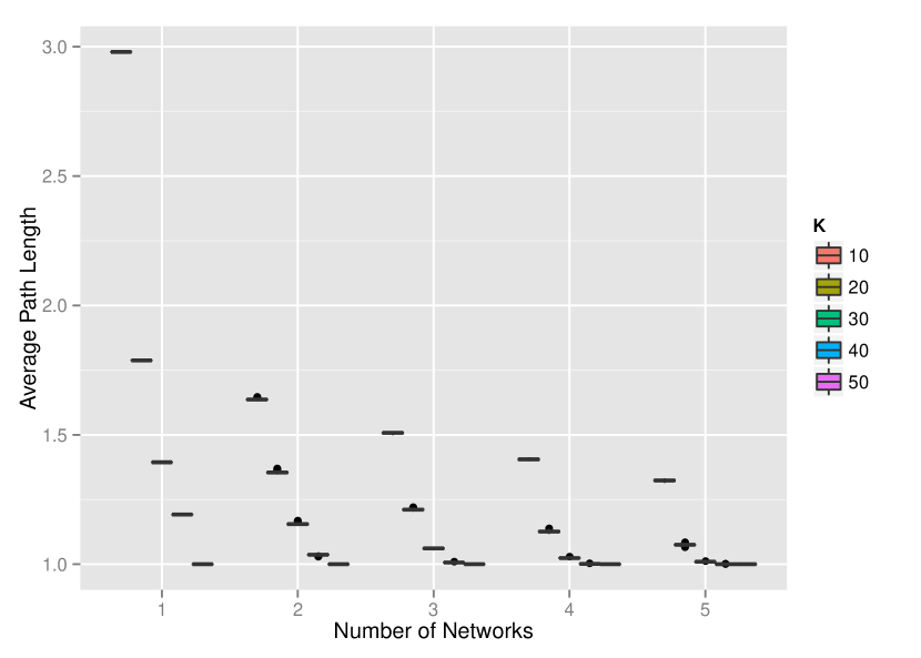
(b)

Figure A.1: Average path length for 100 instances of overlapping k-regular networks(containing 100 nodes each) with  $k=\{1,2,3,4,5\}$ (1(a)), and $k=\{10,20,30,40,50\}$ (1(b)). Since there is barely any variation in the property values for each configuration, the colours cannot be seen correctly, they are presented in the same order as the legend nonetheless.

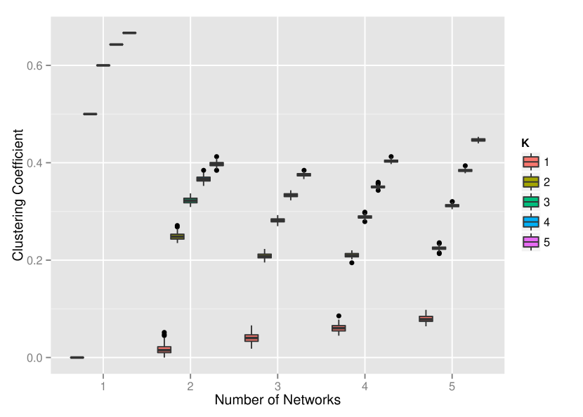
(a)

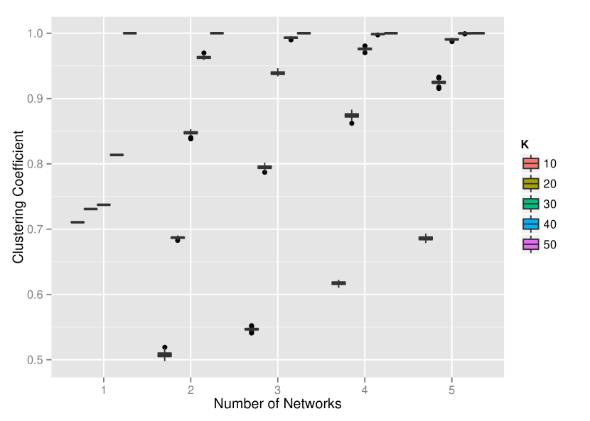
(b)

Figure A.2: Clustering coefficient for 100 instances of overlapping k-regular networks (containing 100 nodes each) with  $k=\{1,2,3,4,5\}$ (2(a)) and $k=\{10,20,30,40,50\}$ (2(b)). Note that the variation is bigger for networks with less connectivity. Also, for $k=50$, the network is fully connected.

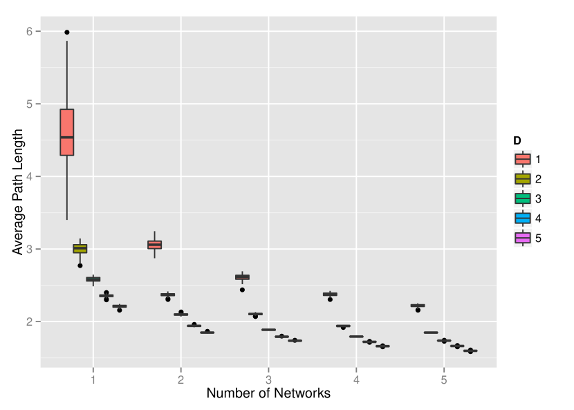
(a) Average path length

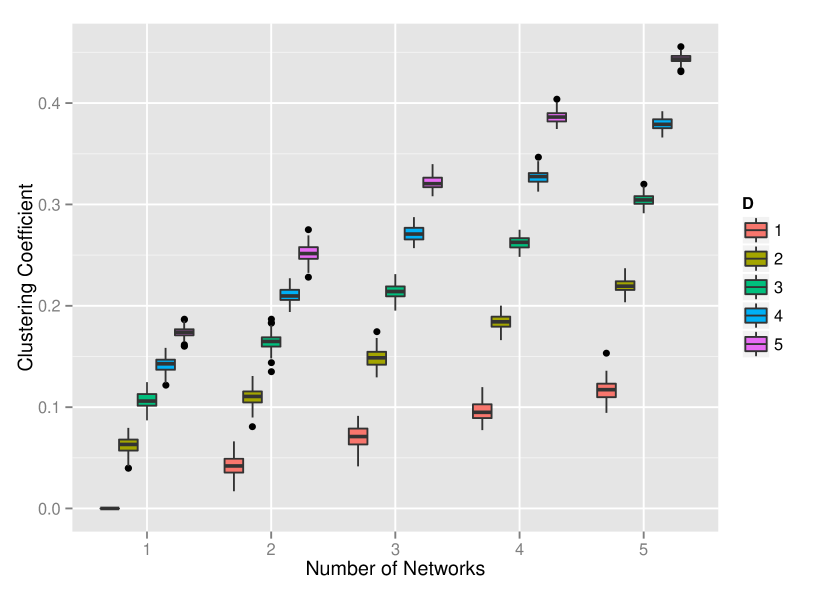
(b) Clustering Coefficient

Figure A.3: Average path length and clustering coefficient for 100 instances of overlapping scale-free networks. D is a parameter used to construct the network. It dictates how many edges are added by preferential attachment each time a new node is added to the networks. For more details refer to [24].

A.2 Heterogeneous Network Topology Configurations

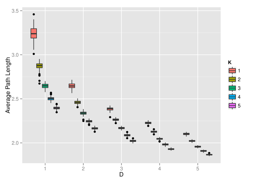
(a)

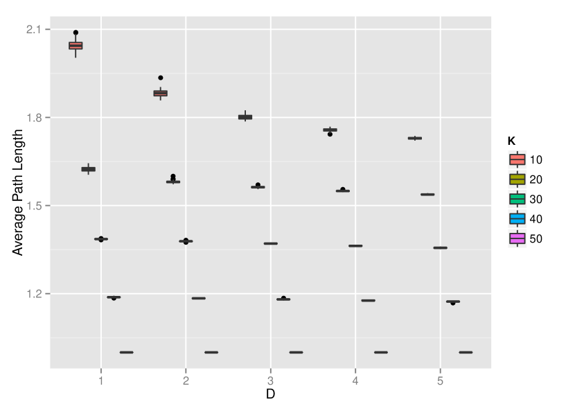
(b)

Figure A.4: Average path length for 100 instances of two overlapping networks: 1 scale-free with $d=\{1,2,3,4,5\}$ and 1 k-regular network with  $k=\{1,2,3,4,5\}$ (4(a)), and $k=\{10,20,30,40,50\}$ (4(b)). Since there is barely any variation in the property values for each configuration, the colours cannot be seen correctly in some cases, they are presented in the same order as the legend nonetheless.

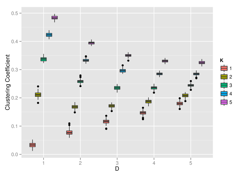
(a)

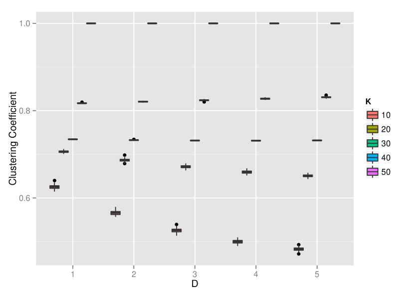
(b)

Figure A.5: Clustering coefficient for 100 instances of two overlapping networks: 1 scale-free with $d=\{1,2,3,4,5\}$ and 1 k-regular network with  $k=\{1,2,3,4,5\}$ (4(a)), and $k=\{10,20,30,40,50\}$ (4(b)). Since there is barely any variation in the property values for each configuration, the colours cannot be seen correctly in some cases, they are presented in the same order as the legend nonetheless.

Appendix B Context Permeability Analysis

Table B.1: Average number of meetings during a simulation run for 100 agents and a maximum of 2000 simulation cycles for different configuration of k-regular networks.

	Number of Networks
	1		2		3		4		5
k	avg.	sd	avg.	sd	avg.	sd	avg.	sd	avg.	sd
1	$200000$	$\phantom{0000}0.0$	$191237$	$35780.6$	$97770$	$86648.0$	$44827$	$71714.8$	$14210$	$31633.6$
2	$200000$	$\phantom{0000}0.0$	$\phantom{0}99744$	$89096.9$	$22690$	$50813.5$	$\phantom{0}7514$	$21352.6$	$\phantom{0}4602$	$\phantom{0}6116.7$
3	$198033$	$19670.0$	$\phantom{0}68555$	$82808.5$	$10217$	$33963.1$	$\phantom{0}6539$	$22227.3$	$\phantom{0}2828$	$\phantom{0}2283.6$
4	$198093$	$19070.0$	$\phantom{0}38359$	$69305.4$	$\phantom{0}5028$	$10680.0$	$\phantom{0}3710$	$\phantom{0}4618.7$	$\phantom{0}2678$	$\phantom{0}2127.4$
5	$196042$	$27845.6$	$\phantom{0}21287$	$48141.1$	$\phantom{0}3444$	$\phantom{0}5144.0$	$\phantom{0}2834$	$\phantom{0}4334.5$	$\phantom{0}2278$	$\phantom{0}1921.5$
10	$178207$	$62301.7$	$\phantom{00}8066$	$28298.4$	$\phantom{0}2894$	$\phantom{0}6424.5$	$\phantom{0}1800$	$\phantom{0}1148.2$	$\phantom{0}2180$	$\phantom{0}2078.3$
20	$\phantom{0}75541$	$95871.3$	$\phantom{00}2338$	$\phantom{0}2739.9$	$\phantom{0}2178$	$\phantom{0}1588.3$	$\phantom{0}1936$	$\phantom{00}989.4$	$\phantom{0}1802$	$\phantom{00}823.6$
30	$\phantom{0}11703$	$43425.0$	$\phantom{00}1952$	$\phantom{0}1087.9$	$\phantom{0}1726$	$\phantom{00}936.6$	$\phantom{0}1930$	$\phantom{0}1096.3$	$\phantom{0}1956$	$\phantom{0}1273.5$
40	$\phantom{00}1694$	$\phantom{00}954.5$	$\phantom{00}1646$	$\phantom{00}821.9$	$\phantom{0}1862$	$\phantom{00}872.3$	$\phantom{0}1806$	$\phantom{00}884.6$	$\phantom{0}1686$	$\phantom{00}647.1$
50	$\phantom{00}1788$	$\phantom{00}786.9$	$\phantom{00}1724$	$\phantom{00}744.7$	$\phantom{0}1776$	$\phantom{00}827.7$	$\phantom{0}1842$	$\phantom{00}896.8$	$\phantom{0}1896$	$\phantom{00}911.4$

Table B.2: Average number of meetings during a simulation run for 100 agents and a maximum of 2000 simulation cycles for different configuration of scale-free networks.

	Number of Networks
	1		2		3		4		5
d	avg.	sd	avg.	sd	avg.	sd	avg.	sd	avg.	sd
1	$200000$	$\phantom{0000}0$	$141085$	$83720$	$66020$	$82601$	$17712$	$42444$	$14917$	$38343.6$
2	$150632$	$78710$	$\phantom{0}21654$	$41341$	$\phantom{0}7555$	$21407$	$\phantom{0}5890$	$10889$	$\phantom{0}3638$	$\phantom{0}5127.0$
3	$\phantom{0}37824$	$64073$	$\phantom{0}12309$	$36441$	$\phantom{0}5299$	$20035$	$\phantom{0}2804$	$\phantom{0}3791$	$\phantom{0}2618$	$\phantom{0}2445.4$
4	$\phantom{0}13751$	$33295$	$\phantom{00}4846$	$\phantom{0}7921$	$\phantom{0}2852$	$\phantom{0}2766$	$\phantom{0}2370$	$\phantom{0}1441$	$\phantom{0}2200$	$\phantom{0}1433.4$
5	$\phantom{00}8802$	$18754$	$\phantom{00}2536$	$\phantom{0}1880$	$\phantom{0}3204$	$11008$	$\phantom{0}2166$	$\phantom{0}1269$	$\phantom{0}1958$	$\phantom{00}971.6$

Table B.3: Average number of meetings during a simulation run for 100 agents and a maximum of 2000 simulation cycles for different configuration of 1 k-regular and 1 scale-free networks.

	d
	1		2		3		4		5
k	avg.	sd	avg.	sd	avg.	sd	avg.	sd	avg.	sd
1	$173312$	$61519$	$100175$	$88406$	$63191$	$81071$	$73715$	$84549$	$51313$	$67704$
2	$118591$	$90107$	$\phantom{0}72054$	$86077$	$43308$	$70318$	$31756$	$58760$	$43281$	$72182$
3	$109155$	$88722$	$\phantom{0}38270$	$66714$	$34899$	$65533$	$26412$	$55589$	$23436$	$49978$
4	$\phantom{0}80035$	$88719$	$\phantom{0}33339$	$64075$	$21289$	$45725$	$15575$	$39516$	$24034$	$52407$
5	$\phantom{0}89179$	$91823$	$\phantom{0}31044$	$62485$	$13908$	$36791$	$14112$	$39490$	$\phantom{0}9252$	$28404$
10	$\phantom{0}62416$	$81036$	$\phantom{0}11017$	$35071$	$\phantom{0}9095$	$27266$	$12182$	$39798$	$\phantom{0}5559$	$20448$
20	$\phantom{0}61371$	$81409$	$\phantom{00}6680$	$17900$	$\phantom{0}6944$	$27826$	$\phantom{0}4721$	$19832$	$\phantom{0}2390$	$\phantom{0}2313$
30	$\phantom{0}51559$	$77468$	$\phantom{00}4980$	$12740$	$\phantom{0}5095$	$20028$	$\phantom{0}2268$	$\phantom{0}1355$	$\phantom{0}2046$	$\phantom{0}1225$
40	$\phantom{0}58625$	$83049$	$\phantom{00}5483$	$20169$	$\phantom{0}2726$	$\phantom{0}3735$	$\phantom{0}2346$	$\phantom{0}1503$	$\phantom{0}2412$	$\phantom{0}1874$
50	$\phantom{0}48702$	$74718$	$\phantom{00}6568$	$22611$	$\phantom{0}2566$	$\phantom{0}1716$	$\phantom{0}2362$	$\phantom{0}1619$	$\phantom{0}1980$	$\phantom{0}1081$

Appendix C Context Switching Analysis

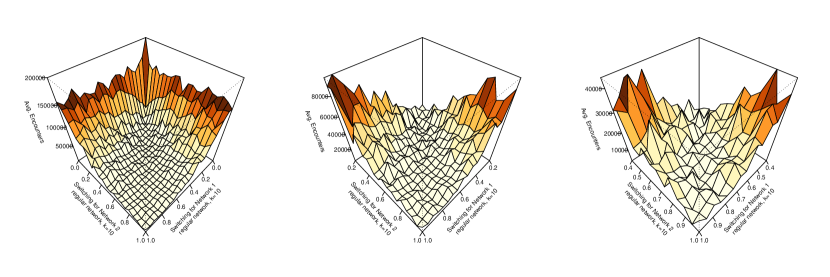
Figure C.1: Perpective plot for the average number of meets during a simulation for 100 independent runs: 2 10-regular networks ($k=30$).

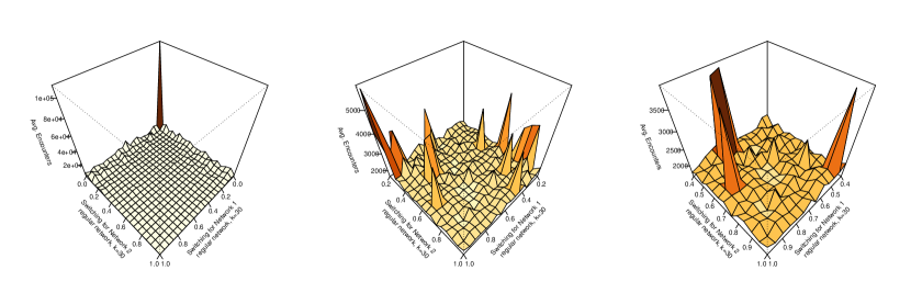
Figure C.2: Perpective plot for the average number of meets during a simulation for 100 independent runs: 2 30-regular networks ($k=30$).

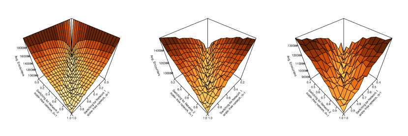
Figure C.3: Perpective plot for the average number of meets during a simulation for 100 independent runs: 2 scale-free networks with $d=1$.

R Figure C.4: Perpective plot for the average number of meets during a simulation for 100 independent runs: 2 scale-free networks with $d=5$.

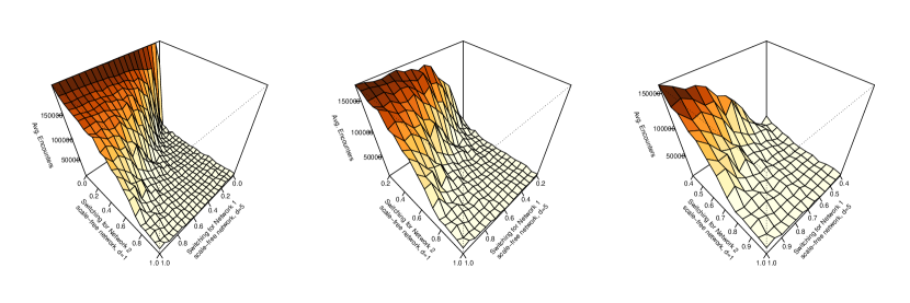
Figure C.5: Perspective plot for the average number of meets during a simulation for 100 independent runs: 2 scale-free networks, the first with $d=5$ and the second with $d=1$.

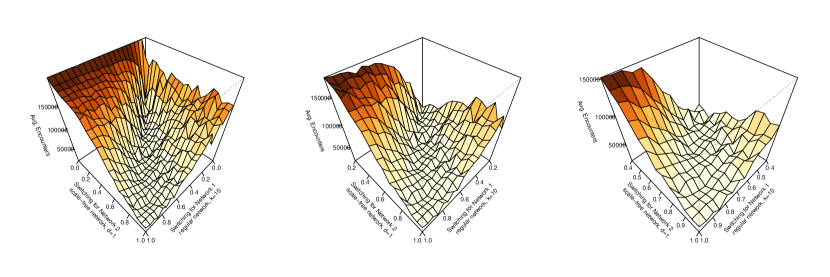
Figure C.6: Perspective plot for the average number of meets during a simulation for 100 independent runs: 1 10-regular network ($k=10$) and a scale-free network with $d=1$.

References

- [1] C. Emmeche, Aspects of complexity in life and science, PHILOSOPHICA-GENT- (1997) 41–68.
- [2] H. A. Simon, Bandwagon and underdog effects and the possibility of election predictions, The Public Opinion Quarterly 18 (3) (1954) pp. 245–253.
- [3] R. Axelrod, The Dissemination of Culture, Journal of Conflict Resolution 41 (2) (1997) 203–226.
- [4] G. Weisbuch, Bounded confidence and social networks, The European Physical Journal B - Condensed Matter and Complex Systems 38 (2004) 339–343.
- [5] P. S. Albin, The analysis of complex socioeconomic systems, Lexington, Mass. : Lexington Books, 1975.
- [6] S. Roccas, M. B. Brewer, Social identity complexity, Personality and Social Psychology Review 6 (2) (2002) 88–106.
- [7] N. Ellemers, R. Spears, B. Doosje, Self and social identity*, Annual Review of Psychology 53 (1) (2002) 161–186.
- [8] J. French, A formal theory of social power, Psychological Review 63 (1956) 181–194.
- [9] M. H. DeGroot, Reaching a Consensus, Journal of the American Statistical Association 69 (345) (1974) 118–121.
- [10] K. Lehrer, Social consensus and rational agnoiology, Synthese 31 (1975) 141–160.
- [11] S. Galam, Rational group decision making: A random field ising model t = 0, Physica A: Statistical Mechanics and its Applications 238 (1) (1997) 66–80.
- [12] L. Antunes, D. Nunes, H. Coelho, J. a. Balsa, P. Urbano, Context Switching versus Context Permeability in Multiple Social Networks, in: Progress in Artificial Intelligence, Vol. 5816 of Lecture Notes in Computer Science, 2009, pp. 547–559.
- [13] G. Deffuant, D. Neau, F. Amblard, G. Weisbuch, Mixing beliefs among interacting agents, Advances in Complex Systems 3 (01n04) (2000) 87–98.
- [14] G. Deffuant, F. Amblard, G. Weisbuch, T. Faure, How can extremism prevail? A study based on the relative agreement interaction model, Journal of Artificial Societies and Social Simulation 5 (4) (2002) 1.
- [15] R. Hegselmann, U. Krause, Opinion dynamics and bounded confidence: models, analysis and simulation, Journal of Artificial Societies and Social Simulation 5 (3) (2002) 2.
- [16] D. K. Lewis, Convention: a philosophical study, Harvard University Press Cambridge, 1969.
- [17] J. Delgado, Emergence of social conventions in complex networks, Artificial intelligence 141 (1) (2002) 171–185.
- [18] Y. Shoham, M. Tennenholtz, Co-learning and the evolution of social activity, Tech. rep., DTIC Document (1994).
- [19] T. C. Schelling, Dynamic models of segregation†, Journal of mathematical sociology 1 (2) (1971) 143–186.
- [20] J. M. Sakoda, The checkerboard model of social interaction, The Journal of Mathematical Sociology 1 (1) (1971) 119–132.
- [21] A. Flache, R. Hegselmann, Do irregular grids make a difference? relaxing the spatial regularity assumption in cellular models of social dynamics., Journal of Artificial Societies and Social Simulation 4 (4).
- [22] D. B. O’Sullivan, Graph-based cellular automaton models of urban spatial processes, Ph.D. thesis, University of London (2000).
- [23] P. Erdős, A. Rényi, On random graphs, Publ. Math. Debrecen 6 (1959) 290–297.
- [24] A. Barabási, R. Albert, Emergence of scaling in random networks, science 286 (5439) (1999) 509.
- [25] D. J. Watts, S. H. Strogatz, Collective dynamics of ’small-world’ networks, Nature 393 (6684) (1998) 440–442.
- [26] M. E. Gaston, M. desJardins, Agent-organized networks for dynamic team formation, in: Proceedings of the fourth international joint conference on Autonomous agents and multiagent systems, ACM, 2005, pp. 230–237.
- [27] D. Nunes, L. Antunes, Consensus by segregation - the formation of local consensus within context switching dynamics, Proceedings of the 4th World Congress on Social Simulation.
- [28] P. J. Hayes, Contexts in context, in: Context in knowledge representation and natural language, AAAI Fall Symposium, 1997.
- [29] L. Antunes, J. Balsa, P. Urbano, H. Coelho, The challenge of context permeability in social simulation, in: Proceedings of the Fourth European Social Simulation Association, 2007.
- [30] L. Antunes, J. Balsa, P. Urbano, H. Coelho, Exploring context permeability in multiple social networks, in: K. Takadama, C. Cioffi-Revilla, G. Deffuant (Eds.), Simulating Interacting Agents and Social Phenomena, Vol. 7 of Agent-Based Social Systems, Springer Japan, 2010, pp. 77–87.
- [31] S. Luke, C. Cioffi-Revilla, L. Panait, K. Sullivan, G. Balan, MASON: A Multiagent Simulation Environment, Simulation 81 (7) (2005) 517–527.
-
[32]
D. Nunes, L. Antunes, Context
Permeability Modelsdoi:{10.5281/zenodo.11067}.
URL {http://dx.doi.org/10.5281/zenodo.11067} -
[33]
R. D. C. Team, R: A Language and Environment
for Statistical Computing, R Foundation for Statistical Computing, Vienna,
Austria, ISBN 3-900051-07-0 (2008).
URL http://www.R-project.org -
[34]
Y. Xie, knitr: A
comprehensive tool for reproducible research in R, in: V. Stodden,
F. Leisch, R. D. Peng (Eds.), Implementing Reproducible Computational
Research, Chapman and Hall/CRC, 2014.
URL http://www.crcpress.com/product/isbn/9781466561595 -
[35]
D. Nunes, L. Antunes, Context
Permeability Analysisdoi:{10.5281/zenodo.11898}.
URL {http://dx.doi.org/10.5281/zenodo.11898} -
[36]
D. Nunes, L. Antunes, B-Have
Network Librarydoi:{10.5281/zenodo.11069}.
URL {http://dx.doi.org/10.5281/zenodo.11069} -
[37]
G. Csardi, T. Nepusz, The igraph software package for
complex network research, InterJournal Complex Systems (2006) 1695.
URL http://igraph.org - [38] S. Tomihisa, K. Kawai, An algorithm for drawing general undirected graphs, Information Processing Letters 31 (1) (1989) 7 – 15. doi:10.1016/0020-0190(89)90102-6.
- [39] D. Villatoro, J. Sabater-Mir, S. Sen, Robust convention emergence in social networks through self-reinforcing structures dissolution, ACM Trans. Auton. Adapt. Syst. 8 (1) (2013) 2:1–2:21. doi:10.1145/2451248.2451250.