Multi-degree bounds on the Betti numbers of real varieties and semi-algebraic sets and applications

Abstract.

We prove new bounds on the Betti numbers of real varieties and semi-algebraic sets that have a more refined dependence on the degrees of the polynomials defining them than results known before. Our method also unifies several different types of results under a single framework, such as bounds depending on the total degrees, on multi-degrees, as well as in the case of quadratic and partially quadratic polynomials. The bounds we present in the case of partially quadratic polynomials offer a significant improvement over what was previously known. Finally, we extend a result of Barone and Basu on bounding the number of connected components of real varieties defined by two polynomials of differing degrees to the sum of all Betti numbers, thus making progress on an open problem posed in that paper.

1. Introduction

Throughout this paper $\mathrm{R}$ will denote a fixed real closed field and $\mathrm{C}$ the algebraic closure of $\mathrm{R}$. For any semi-algebraic subset $S\subset\mathrm{R}^{k}$ we denote by $b_{i}(S,\mathbb{Z}_{2})$ the dimension of the $i$-th homology group, $\mbox{\rm H}_{i}(S,\mathbb{Z}_{2})$, and by $b(S,\mathbb{F})=\sum_{i\geq 0}b_{i}(S,\mathbb{F})$ (we refer the reader to [17, Chapter 6] for definition of homology groups of semi-algebraic sets defined over arbitrary real closed fields).

Remark 1.

Notice that by the universal coefficient theorem [43, page 222], $b_{i}(S,\mathbb{Z}_{2})\geq b_{i}(S)$ (where $b_{i}(S)$ denotes the rank of the $i$-th homology group of $S$ with integer coefficients), and thus an upper bound on $b_{i}(S,\mathbb{Z}_{2})$ is automatically an upper bound on $b_{i}(S)$.

1.1. Background

The problem of bounding the Betti numbers of real algebraic varieties as well as semi-algebraic subsets of $\mathrm{R}^{k}$, in terms of the format of their defining formulas, has been an active topic of investigation for a long time starting from the first results bounding the Betti numbers of real varieties proved by Oleĭnik and Petrovskiĭ [40], Thom [44] and Milnor [38]. Later these results were extended to more general semi-algebraic sets [11, 26, 27]. These results were based on Morse-theoretic arguments involving bounding the number of critical points of a Morse function on a bounded, non-singular real algebraic hypersurface, using Bezout’s theorem, arguments involving infinitesimal perturbations, and use of inequalities coming from the Mayer-Vietoris exact sequence. The bounds were singly exponential in the dimension of the ambient space and polynomial in the number of polynomials used in the definition of the given semi-algebraic set, and also in the maximum of the total degrees of these polynomials (see Theorems 1, 2, 3, below for precise statements).

In another direction, bounds which are polynomial in the dimension were proved for a restricted class of semi-algebraic sets – namely, semi-algebraic sets defined by few (i.e,. a constant number of) quadratic equalities and inequalities. Barvinok [10] proved a polynomial bound on the Betti numbers of semi-algebraic sets (see Theorem 4 for a precise statement), which were sharpened in [14, 36], and also extended to a more general setting in [15] (see Theorem 8 for a precise statement). Some of these results were proved using different techniques than a simple counting of critical points – for example, a spectral sequence argument first proposed by Agrachev [3, 2, 5] plays an important role in the results proved in [15, 36].

Much more recently, because of certain new techniques developed in incidence geometry, more refined bounds than those mentioned above were needed. In particular, it was not enough to prove bounds which depended on the maximum of the degrees of the polynomials, and it was necessary to prove bounds with a more refined dependence on the sequence of degrees. Nearly optimal bounds on the zero-th Betti numbers (i.e. the number of connected components) of semi-algebraic sets was proved later in [7, 8] which has proved useful in applications. However, the techniques used to prove the results in [7, 8] are not sufficient for bounding the higher Betti numbers. Extending the bounds proved in [7, 8] to the sum of all the Betti numbers (i.e. not just the zero-th Betti number) remains a challenging open problem in real algebraic geometry.

The main contributions of the current paper are as follows. The first contribution is to develop a single framework which allows one to prove the bounds on general semi-algebraic sets, as well as those defined by quadratic or even partially quadratic polynomials (Theorems 11, 16, 17, 18, 19). Moreover, we improve the known bounds in all of these cases. In the process, we also answer an open question of Lerario [36] on the asymptotic behavior of the Betti numbers of complete intersections of projective quadrics over $\mathrm{C}$ and $\mathrm{R}$ (Theorems 17 and 25).

Additionally, the framework allows us to prove bounds in terms of the multi-degrees of the polynomials instead of the total degrees (Theorems 12, 13, 14, 15, 20, 21). We give several applications in which this new flexibility proves to be important (Theorems 26, 27, 28, 29). Note that there have been some other applications of multi-degree bounds in special cases (see for instance [31] for a recent algorithmic application).

As mentioned above, extending the bounds proved in [7, 8] to the sum of all the Betti numbers remains an open problem. The second contribution of the current paper is extending the result [7] to the sum of all the Betti numbers to the case of degree sequence of length bounded by $2$ (Theorems 31 and 32), thereby making progress on the open problem posed in [8].

1.2. Prior Results

In this section we state more precisely the prior results mentioned in the previous section. We first fix some notation that we will use for the rest of the paper.

1.2.1. Basic notation and definition

Notation 1.

For $P\in\mathrm{R}[X_{1},\ldots,X_{k}]$ (resp. $P\in\mathrm{C}[X_{1},\ldots,X_{k}]$) we denote by $\mathrm{Zer}(P,\mathrm{R}^{k})$ (resp. $\mathrm{Zer}(P,\mathrm{C}^{k})$) the set of zeros of $P$ in $\mathrm{R}^{k}$(resp. $\mathrm{C}^{k}$). More generally, for any finite set $\mathcal{P}\subset\mathrm{R}[X_{1},\ldots,X_{k}]$ (resp. $\mathcal{P}\subset\mathrm{C}[X_{1},\ldots,X_{k}]$), we denote by $\mathrm{Zer}(\mathcal{P},\mathrm{R}^{k})$ (resp. $\mathrm{Zer}(\mathcal{P},\mathrm{C}^{k})$) the set of common zeros of $\mathcal{P}$ in $\mathrm{R}^{k}$ (resp. $\mathrm{C}^{k}$). For a homogeneous polynomial $P\in\mathrm{R}[X_{0},\ldots,X_{k}]$, (resp. $P\in\mathrm{C}[X_{0},\ldots,X_{k}]$) we denote by $\mathrm{Zer}(P,\mathbb{P}_{\mathrm{R}}^{k})$ (resp. $\mathrm{Zer}(P,\mathbb{P}_{\mathrm{C}}^{k})$) the set of zeros of $P$ in $\mathbb{P}_{\mathrm{R}}^{k}$. (resp. $\mathbb{P}_{\mathrm{C}}^{k}$). And, more generally, for any finite set of homogeneous polynomials $\mathcal{P}\subset\mathrm{R}[X_{0},\ldots,X_{k}]$, (resp. $\mathcal{P}\subset\mathrm{C}[X_{0},\ldots,X_{k}]$), we denote by $\mathrm{Zer}(\mathcal{P},\mathbb{P}_{\mathrm{R}}^{k})$ (resp. $\mathrm{Zer}(\mathcal{P},\mathbb{P}_{\mathrm{C}}^{k})$) the set of common zeros of $\mathcal{P}$ in $\mathbb{P}_{\mathrm{R}}^{k}$. (resp. $\mathbb{P}_{\mathrm{C}}^{k}$).

Notation 2.

For any finite family of polynomials $\mathcal{P}\subset\mathrm{R}[X_{1},\ldots,X_{k}]$, we call an element $\sigma\in\{0,1,-1\}^{\mathcal{P}}$, a sign condition on $\mathcal{P}$. For any semi-algebraic set $Z\subset\mathrm{R}^{k}$, and a sign condition $\sigma\in\{0,1,-1\}^{\mathcal{P}}$, we denote by $\mathrm{Reali}(\sigma,Z)$ the semi-algebraic set defined by

$$\{\mathbf{x}\in Z\mid\mbox{\bf sign}(P(\mathbf{x}))=\sigma(P),P\in\mathcal{P}\},$$

and call it the realization of $\sigma$ on $Z$. More generally, we call any Boolean formula $\Phi$ with atoms, $P\{=,>,<\}0,P\in\mathcal{P}$, to be a $\mathcal{P}$-formula. We call the realization of $\Phi$, namely the semi-algebraic set

$$\mathrm{Reali}\left(\Phi,\mathrm{R}^{k}\right) = \left\{\mathbf{x}\in\mathrm{R}^{k}\mid\Phi(\mathbf{x})\right\}$$

a $\mathcal{P}$-semi-algebraic set. Finally, we call a Boolean formula without negations, and with atoms $P\{\geq,\leq\}0$, $P\in\mathcal{P}$, to be a $\mathcal{P}$-closed formula, and we call the realization, $\mathrm{Reali}\left(\Phi,\mathrm{R}^{k}\right)$, a $\mathcal{P}$-closed semi-algebraic set.

1.2.2. General Bounds

The first results on bounding the Betti numbers of real varieties were proved by Oleĭnik and Petrovskiĭ [40], Thom [44] and Milnor [38]. Using a Morse-theoretic argument and Bezout’s theorem they proved:

Theorem 1.

[40, 44, 38] Let $\mathcal{Q}\subset\mathrm{R}[X_{1},\ldots,X_{k}]$ with $\deg(Q)\leq d,Q\in\mathcal{Q}$. Then,

(1.1) $$b(\mathrm{Zer}(\mathcal{Q},\mathrm{R}^{k}),\mathbb{Z}_{2})\leq d(2d-1)^{k-1}.$$

Remark 2.

Theorem 1 is proved (see for example proof of Theorem 11.5.3 in [20] for an exposition) by first replacing the given variety by a bounded basic, closed semi-algebraic set having the same homotopy type as $\mathrm{Zer}(\mathcal{Q},\mathrm{R}^{k})$ defined by a single polynomial inequality of total degree at most twice the maximum of the degrees of the polynomials in $\mathcal{Q}$. Moreover, the critical points of the coordinate function $X_{1}$ are shown to be non-degenerate and their number can be bounded using Bezout’s theorem.

Remark 3.

Also, note that the bound in Theorem 1 holds for dimensions of the homology groups with coefficients in any field and was proved in that generality. The same is true for some of the other results surveyed below. However, the new results in this paper give bounds only for Betti numbers over the field $\mathbb{Z}_{2}$ (because our technique for proving them involves using Smith inequalities cf. Theorem 22), and are thus correspondingly weaker. On the other hand they do imply via the universal coefficients theorem (see Remark 1) the same bounds on the ranks of the homology groups with integer coefficients. Moreover, $\mathbb{Z}_{2}$-homology is very natural in the context of real algebraic geometry. We will state all bounds for the $\mathbb{Z}_{2}$-Betti numbers from now on without comment (except in §6 below).

Theorem 1 was later generalized to arbitrary semi-algebraic sets defined by quantifier-free formulas in two steps. In the first step, Theorem 1 was extended to a particular – namely $\mathcal{P}$-closed semi-algebraic sets, where $\mathcal{P}\subset\mathrm{R}[X_{1},\ldots,X_{k}]$ is a finite family of polynomials. The following theorem (which makes more precise an earlier result appearing in [11]) appears in [16].

Theorem 2.

[16] If $S\subset\mathrm{R}^{k}$ is a $\mathcal{P}$-closed semi-algebraic set, then

(1.2) $$b(S,\mathbb{Z}_{2})\leq\sum_{i=0}^{k}\sum_{j=0}^{k-i}\binom{s+1}{j}6^{j}d(2d-1)^{k-1},$$

where $s=\mathrm{card}(\mathcal{P})>0$ and $d=\max_{P\in\mathcal{P}}\deg(P)$.

Using an additional ingredient (namely, a technique to replace an arbitrary semi-algebraic set by a locally closed one with a very controlled increase in the number of polynomials used to describe the given set), Gabrielov and Vorobjov [26] extended Theorem 2 to arbitrary $\mathcal{P}$-semi-algebraic sets with only a small increase in the bound. Their result in conjunction with Theorem 2 gives the following theorem.

Theorem 3.

[27] If $S\subset\mathrm{R}^{k}$ is a $\mathcal{P}$-semi-algebraic set, then

(1.3) $$b(S,\mathbb{Z}_{2})\leq\sum_{i=0}^{k}\sum_{j=0}^{k-i}\binom{2ks+1}{j}6^{j}d(2d-1)^{k-1},$$

where $s=\mathrm{card}(\mathcal{P})$ and $d=\max_{P\in\mathcal{P}}\deg(P)$.

1.2.3. Quadratic and partially quadratic case

Semi-algebraic sets defined by few quadratic inequalities are topologically simpler. This was first noticed by Agrachev [3, 2, 5] who proved a bound which is polynomial in the number of variables and exponential in the number of inequalities for generic quadratic inequalities. The technique introduced by Agrachev was very important in later developments as well. Independently, using a different technique (closer to the spirit of Morse theoretic arguments) Barvinok [10] proved the following theorem (no genericity assumption is required).

Theorem 4.

[10] Let $S\subset\mathrm{R}^{k}$ be defined by $P_{1}\geq 0,\ldots,P_{s}\geq 0,\;\deg(P_{i})\leq 2,\;1\leq i\leq s$. Then,

$$b(S,\mathbb{Z}_{2})\leq k^{O(s)}.$$

This bound was later sharpened in [14] and further sharpened in the case of algebraic sets by Lerario in [36, Theorem 15], where the following nearly optimal result was proved.

Theorem 5.

[36] Let $\mathcal{Q}\subset\mathrm{R}[X_{0},\ldots,X_{k}]$ be a set of $\ell$ quadratic forms, and $V=\mathrm{Zer}(\mathcal{Q},\mathbb{P}_{\mathrm{R}}^{k})$ be the projective variety defined by $\mathcal{Q}$. Then,

$$b(V,\mathbb{Z}_{2})\leq(O(k))^{\ell-1}.$$

Theorem 4 was later extended in [13] where the following theorem was proved. Notice that this bound is polynomial even in the number of inequalities (for fixed $\ell$).

Theorem 6.

[13] Let $\ell$ be any fixed number and let $\mathrm{R}$ be a real closed field. Let $S\subset\mathrm{R}^{k}$ be defined by $P_{1}\geq 0,\ldots,P_{s}\geq 0,\;\deg(P_{i})\leq 2$. Then,

$$b_{k-\ell}(S,\mathbb{Z}_{2})\leq\binom{s}{\ell}k^{O(\ell)}.$$

Theorem 6 was further improved using bounds on the Betti numbers of non-singular complete intersections and the Smith inequality (Theorem 22) in [14] where the following theorem is proved.

Theorem 7.

[14] Let $\mathcal{P}=\{P_{1},\ldots,P_{s}\}\subset\mathrm{R}[X_{1},\ldots,X_{k}],\;s\leq k$. Let $S\subset\mathrm{R}^{k}$ be defined by

$$P_{1}\geq 0,\ldots,P_{s}\geq 0$$

with $\deg(P_{i})\leq 2$. Then, for $0\leq i\leq k-1$,

$$b_{i}(S,\mathbb{Z}_{2})\leq\frac{1}{2}\left(\sum_{j=0}^{min\{s,k-i\}}\binom{s}{j}\binom{k+1}{j}2^{j}\right).$$

In particular, for $2\leq s\leq k/2$, we have

$$b_{i}(S,\mathbb{Z}_{2})\leq\frac{1}{2}3^{s}\binom{k+1}{s}\leq\frac{1}{2}\left(\frac{3e(k+1)}{s}\right)^{2}.$$

Finally, in [15] the authors also prove a result that generalizes the bounds on Betti numbers of general semi-algebraic sets (defined by $s$ polynomials having degrees bounded by $d$, cf. Theorem 2), as well as the bounds in the quadratic case (cf. Theorems 4, 6, and 7). More precisely they prove:

Theorem 8.

[15] Let $\mathcal{P}_{1}\subset\mathrm{R}[X_{1},\ldots,X_{k_{1}}]$, a finite set of polynomials with

$$\deg_{X}(P)\leq d,P\in\mathcal{P}_{1},\mathrm{card}({\mathcal{P}}_{1})=s,$$

and let $\mathcal{P}_{2}\subset\mathrm{R}[X_{1},\ldots,X_{k_{1}},Y_{1},\ldots,Y_{k_{2}}]$, a finite set of polynomials with

$$\deg_{X}(P)\leq d,\deg_{Y}(P)\leq 2,P\in\mathcal{P}_{2},\mathrm{card}(\mathcal{P}_{2})=m,$$

Let $S\subset\mathrm{R}^{k_{1}+k_{2}}$ be a $(\mathcal{P}_{1}\cup\mathcal{P}_{2})$-closed semi-algebraic set. Then

(1.4) $$b(S,\mathbb{Z}_{2}) \leq k_{2}^{2}(O(k_{2}+s+m)k_{2}d)^{k_{1}+2m}.$$

In particular, for $m\leq k_{2}$, $\displaystyle{b(S,\mathbb{Z}_{2})\leq k_{2}^{2}(O(s+k_{2})k_{2}d)^{k_{1}+2m}.}$

Remark 4.

In particular, if in Theorem 8, $\mathcal{P}_{1}=\emptyset$ (and hence $s=0$), and $m,k_{1}<k_{2}$, we get

(1.5) $$b(S,\mathbb{Z}_{2}) \leq k_{2}^{2}(O(m+k_{2})k_{2}d)^{k_{1}+2m}.$$

Remark 5.

The main tool used in the proof of Theorem 8 was a technique introduced by Agrachev in [5, 2, 3] and later exploited by several authors [15, 4, 35, 36] for bounding the Betti numbers of semi-algebraic sets defined by quadratic polynomials.

The techniques used in the proof of the theorems corresponding to Theorem 8 in the current paper (namely, Theorems 16, 18, and 19) are quite different – involving the method of infinitesimal perturbations, Mayer-Vietoris inequalities as explained in [17, Chapter 7], and bounds on the Betti numbers of real affine varieties defined by partially quadratic polynomials proved in Proposition 12 below.

1.2.4. Generic vs special

Definition 1 (Generic).

In this paper while considering tuples of polynomials $(P_{1},\ldots,P_{\ell})$ whose supports are contained in some fixed tuple of convex polytopes $\boldsymbol{\Delta}=(\Delta_{1},\ldots,\Delta_{\ell})$ we will often make the assumption that the polynomials in the system are generic. This means that the vector of coefficients of $(P_{1},\ldots,P_{\ell})$ lie outside of some Zariski-closed subset, $V_{\boldsymbol{\Delta}}$, of strictly positive codimension in the vector space of coefficients of the polynomial system (the Zariski-closed subset $V_{\boldsymbol{\Delta}}$ will depend on $\boldsymbol{\Delta}$).

Since the intersection of a Zariski-closed subset of $\mathrm{C}^{N}$ of strictly positive codimension with $\mathrm{R}^{N}\subset\mathrm{C}^{N}$ is a Zariski-closed subset of $\mathrm{R}^{N}$ of strictly positive (real) codimension, while considering systems of generic complex polynomials, we can always assume that the coefficients belong to $\mathrm{R}$. However, note that in the complex case since the discriminant hypersurface does not disconnect the space of coefficients, the varieties defined by generic systems are all diffeomorphic to each other, the same is clearly not always true for the real parts of such varieties.

In many quantitative results in algebraic geometry, one assumes that the given system of polynomials is generic. Bounding the topological complexity of varieties defined by generic systems of polynomials (over $\mathrm{R}$ as well as $\mathrm{C}$) is often easy. However, such a result does not imply a bound in the non-generic situation. The following example which appears in [25] is very well-known and shows that even for the zero-th Betti number, the “generic” bound might not hold for all special systems.

Example 1.

[25] Let $k=3$ and let

$$Q_{1} = X_{3},$$

$$Q_{2} = X_{3},$$

$$Q_{3} = \sum_{i=1}^{2}\left(\prod^{d}_{j=1}(X_{i}-j)^{2}\right).$$

The real variety defined by $\mathcal{Q}=\{Q_{1},Q_{2},Q_{3}\}$ is $0$-dimensional, and has $d^{2}$ isolated (in $\mathrm{R}^{3}$) points. However, a “generic” system of three polynomials in $\mathrm{R}[X_{1},X_{2},X_{3}]$ having degrees $1,1,2d$ will have by Bezout’s theorem at most $2d$ isolated points as its real zeros. Observe that even though the real variety $\mathrm{Zer}(\mathcal{Q},\mathrm{R}^{3})$ is zero-dimensional, the complex variety $\mathrm{Zer}(\mathcal{Q},\mathrm{C}^{3})$ is not, which accounts for this discrepancy. We refer the reader to [8] for a Bezout-type inequality that works over $\mathrm{R}$ as well.

There has been some work on bounding the number of connected components of real algebraic varieties defined by systems of polynomials satisfying certain genericity conditions. For example, the following theorem appears in [23].

Theorem 9.

[23] Let $(P_{1},\ldots,P_{s})\subset\mathbb{Q}[X_{1},\ldots,X_{k}]$ (with $s\leq k-1$) generate a radical ideal and define a smooth algebraic variety $V\subset\mathrm{C}^{k}$ of dimension $k^{\prime}$. Denote by $d_{1},\ldots,d_{s}$ the respective degrees of $P_{1},\ldots,P_{s}$ and by $d$ the maximum of $d_{1},\ldots,d_{s}$. The number of connected components of $V\cap\mathrm{R}^{k}$ is bounded by

$$d_{1}\cdots d_{s}\sum_{i=0}^{k^{\prime}}(d-1)^{k-s-i}\binom{k-i}{k-i-s}.$$

Moreover, if $(P_{1},\ldots,P_{s})$ is a regular sequence, the number of connected components of $V\cap\mathrm{R}^{k}$ is bounded by

$$d_{1}\cdots d_{s}\sum_{i=0}^{k^{\prime}}(d-1)^{k-s-i}\binom{k-i-1}{k-i-s}.$$

Even though, bounds on generic systems do not immediately produce a bound on the Betti numbers of general semi-algebraic sets, but with extra effort such bounds can be used to prove (possibly worse) bounds for general semi-algebraic sets. This is in fact the approach taken in this paper, but the approach already appears in the paper by Benedetti, Loeser and Risler [19], which is the starting point of the results presented in the current paper. Using a clever reduction from the general case to the generic case they prove the following theorem.

Theorem 10.

[19, Proposition 2.6] Let $\mathcal{P}=\{P_{1},\ldots,P_{\ell}\}$ with $\deg(P_{i})\leq d,\;1\leq i\leq\ell,\;P_{i}\in\mathrm{R}[X_{1},\ldots,X_{k}]$. Then,

$$b_{0}(\mathrm{Zer}(\mathcal{P},\mathrm{R}^{k}),\mathbb{Z}_{2})\leq\lambda(d,k,\ell),$$

where

$$\lambda(d,k,\ell)=Q_{1}(d,k)+2Q_{2}(d,k)+\cdots+2^{k-\ell-1}Q_{k-\ell}(d,k)+2^{k-\ell}\mu_{d}(\ell),$$

and each $Q_{i}$ is a polynomial in $d$ of degree $k-i+1$, the leading coefficient of $Q_{1}$ is a polynomial in $k$ of degree $\ell-1$ with leading coefficient $(\ell+1)/2$, and the other terms polynomials in $k$ of degree $\max\{\ell-1,1\}$, and $\mu_{d}(\ell)=d(2d-1)^{\ell-1}$.

Remark 6.

Of special interest here is that for every fixed $\ell$, and $k$ large enough (depending on $\ell$), and for $d$ tending to infinity, $\lambda(d,k,\ell)$ is asymptotically equal to $\left(\frac{1}{2}(\ell+1)k^{\ell-1}+O_{\ell}(k^{\ell-2})\right)d^{k}+O_{k,\ell}(d^{k-1})$ [19, Corollary 2.7] where the implied constant in the notation $O_{\ell}$ (resp. $O_{k,\ell}$) depends only on $\ell$ (resp. $k,\ell$) (compare with Theorem 11 and Remark 7 below).

In this paper, we consider the problem of bounding the sum of all the Betti numbers of real varieties and semi-algebraic sets with a more refined dependence on the degrees of the polynomials. These refinements are of two kinds. First, we allow different blocks of variables to have different degrees (see Theorems 12 and 13). Second, we allow different polynomials to have different degrees (see Theorems 14 and 15). Using our techniques we also improve existing bounds on the sum of the Betti numbers of real varieties and semi-algebraic sets in terms of the number and total degrees of polynomials defining them (Theorem 11) as well as in the partially quadratic case (Theorems 16, 17, 18, 19, 20, and 21).

The results mentioned above are all proved using a single framework, which can be summarized as follows. Using infinitesimal perturbation and inequalities derived from the Mayer-Vietoris exact sequence, we reduce the problem of bounding the sum of the $\mathbb{Z}_{2}$-Betti numbers of a particular class of semi-algebraic sets to bounding the same for a set of real algebraic varieties, which are non-singular complete intersections in affine space. The perturbations need to be chosen carefully so that the degree dependencies of the various blocks of variables in the original set of polynomials are preserved. We then use Smith inequalities and a result of Khovanskiĭ [32] to bound the $\mathbb{Z}_{2}$-Betti numbers of these varieties.

We apply the results mentioned above to prove refined bounds on the Betti numbers of pull-backs and direct images under polynomial maps (Theorems 26, 27, 28), and as an application of the last result (i.e. Theorem 28) give a better bound (than possible before) on the Betti numbers of the space of affine subspaces of a fixed dimension that meet a given semi-algebraic subset of $\mathrm{R}^{k}$ (related to an important problem studied in discrete geometry). Finally, we make some progress on extending the theorem on refined bounds on the number of connected components of real varieties defined by polynomials having different degrees, to a bound on the sum of the Betti numbers using results proved in this paper and some other ingredients (namely stratified Morse theory and Lefschetz duality from topology of manifolds). This is reported in Theorem 32.

The rest of the paper is organized as follows. In §2 we state the main results proved in this paper. In §3, we state some preliminary results that are needed in the proofs of the main theorems. In §4, we prove the main theorems of the paper. In §5, we prove bounds on the Betti numbers of pull-backs, direct images, and the space of transversals of semi-algebraic sets. In §6, we prove a refined bound on the Betti numbers of varieties defined by polynomials having two different degree bounds. Finally, in §7 we list some open problems and possible future research directions.

2. Main Results

2.1. Betti numbers of sets defined by polynomials of bounded total degree

We begin with the classical case of bounding the sum of the Betti numbers of varieties and semi-algebraic sets in terms of the total degrees of the polynomials defining them. This is the classical situation already considered by many authors and already surveyed in §1.2, but our methods produce slight improvements which we record here. We prove the following theorems.

Theorem 11.

Let $\mathcal{Q}=\{Q_{1},\ldots,Q_{\ell}\}\subset\mathrm{R}[X_{1},\ldots,X_{k}]$ be a finite set of polynomials whose (total) degrees are bounded by $d$ with $\ell>0$. Let $V$ denote $\mathrm{Zer}(\mathcal{Q},\mathrm{R}^{k})$. Then, $b(V,\mathbb{Z}_{2})$ is bounded by

(2.1) $$\min\left(\sum_{j=1}^{k-1}\binom{\ell}{j}2^{j}(F_{1}(d^{\prime},k,j)+F_{2}(d^{\prime},k,j))+\binom{\ell}{k}2^{k}d^{\prime k}+3,\frac{1}{2}(1+(2d-1)^{k})\right),$$

where

$$F_{1}(d^{\prime},k,j) = 1+(-1)^{k-j+1}+$$

$$2d^{\prime j-1}\cdot\left(\sum_{h=0}^{k-j}\sum_{i=0}^{h}(-1)^{k-j+h}\binom{k}{h+j}\binom{j+i-2}{i}2^{h-i}d^{\prime i}\right)$$

$$\leq 2\binom{k-2}{j-2}d^{k-1}+(O(d))^{k-2},$$

$$F_{2}(d,k,j) = 1+(-1)^{k-j+1}+\binom{k-1}{j-1}(d^{\prime k}+k-1)$$

$$\leq \binom{k-1}{j-1}d^{k}+O(1)^{k},$$

and $d^{\prime}$ is the least even integer $\geq d$.

In particular, if $k$ is fixed and $\ell\leq k$, then for large $d$ we have

(2.2) $$b(V,\mathbb{Z}_{2}) \leq \sum_{j=1}^{\ell}2^{j}\binom{\ell}{j}\binom{k-1}{j-1}d^{k}+(O(d))^{k-1}.$$

Remark 7.

Writing the bound in Theorem 11 as a polynomial in $d$, the leading coefficient is

$$\sum_{j=1}^{\ell}2^{j}\binom{\ell}{j}\binom{k-1}{j-1} \leq (3^{\ell}-1)\left(\sum_{j=1}^{\ell}\binom{k-1}{j-1}\right)$$

$$\leq \ell(3^{\ell}-1)\binom{k-1}{\ell-1}\mbox{ for }\ell<k/2.$$

Thus, for every fixed $\ell$ and every $k$ sufficiently large (depending on $\ell$), and as $d$ tends to infinity, the bound in (2.2) is asymptotically equal to

$$\left(\frac{\ell(3^{\ell}-1)}{(\ell-1)!}k^{\ell-1}+O_{\ell}(k^{\ell-2})\right)d^{k}+O_{k,\ell}(d^{k-1}),$$

where the implied constant in the notation $O_{\ell}$ (resp. $O_{k,\ell}$) depends only on $\ell$ (resp. $k,\ell$). Notice that for $\ell>8$,

$$\frac{\ell(3^{\ell}-1)}{(\ell-1)!}<\frac{1}{2}(\ell+1)$$

(cf. Remark 6 following Theorem 10). Thus, for fixed $\ell$ and $k$ (sufficiently large) the bound in Theorem 11 is asymptotically better (as $d$ tends to infinity) than the bound in Theorem 10. Indeed the leading coefficient, $\frac{\ell(3^{\ell}-1)}{(\ell-1)!}$, in the bound in Theorem 11 tends to $0$ exponentially fast with $\ell$, in contrast to the leading coefficient in the bound in Theorem 10.

Remark 8.

Notice that the bound in Theorem 11 is strictly better than the Oleĭnik-Petrovskiĭ-Thom-Milnor bound (Theorem 1) for all values of $\ell,d$ and $k$, with $d,k>1$, with equality in the case $d=1$ or $k=1$. Assuming that $d,k>1$, we have that

$$\frac{1}{2}(1+(2d-1)^{k})<d(2d-1)^{k-1}$$

since

$$1+(2d-1)^{k}<(2d-1)^{k-1}+(2d-1)^{k}=2d(2d-1)^{k-1}.$$

Remark 9.

Even though the results are incomparable, it is still interesting to note that using earlier results of Adolphson and Sperber [1] (who used methods involving bounding exponential sums) Katz [33] proved a bound of

(2.3) $$6\cdot 2^{r}\cdot(2+(1+rd))^{k+1}$$

on $\sum_{i\geq 0}\dim_{\mathbb{Q}_{\ell}}\mbox{\rm H}^{i}_{c}(V,\mathbb{Q}_{\ell})$ (here $\mbox{\rm H}_{c}^{*}(V,\mathbb{Q}_{\ell})$ denotes the $\ell$-adic cohomology groups with compact support), where $V\subset\mathrm{C}^{k}$ is an affine variety defined by $r$ polynomials in $\mathrm{C}[X_{1},\ldots,X_{k}]$ of total degrees bounded by $d$. While this result is incomparable with the results proved in this paper, and cannot be derived using our methods, notice that the bound in (2.3) has an exponent of $k+1$ which is worse than the bound in Theorem 11 (in the case $\ell,k$ are fixed and $d$ is large).

2.2. Betti numbers of sets defined by polynomials of bounded multi-degrees

We now consider the multi-degree case.

Notation 3.

Given, $\mathbf{k}=(k_{1},\ldots,k_{p}),\mathbf{d}=(d_{1},\ldots,d_{p})\in\mathbb{N}^{p},k=\sum_{i=1}^{p}k_{i}$, and $j>0$, we denote:

$$G_{\mathrm{gen}}(\mathbf{d},\mathbf{k},j)=1+(-1)^{k-j+1}+(k-j+2)^{2}\binom{k}{j-1}\binom{k}{\mathbf{k}}^{-1}\frac{(1+p)^{3k-j+1}}{p(p+2)}d_{1}^{k_{1}}\cdots d_{p}^{k_{p}}.$$

Theorem 12.

Let $\mathcal{Q}=\{Q_{1},\ldots,Q_{\ell}\}\subset\mathrm{R}[\mathbf{X}^{(1)},\ldots,\mathbf{X}^{(p)}]$ be a finite set of polynomials with $\ell>0$, where for $1\leq i\leq p$, $\mathbf{X}^{(i)}=(X^{(i)}_{1},\ldots,X^{(i)}_{k_{i}})$, and $\deg_{\mathbf{X}^{(i)}}(Q)\leq d_{i},\;d_{i}\geq 2$, for all $Q\in\mathcal{Q}$. Let also $V=\mathrm{Zer}(\mathcal{Q},\mathrm{R}^{k})$, where $k=\sum_{i=1}^{p}k_{i}$. Denote by $\mathbf{d}=(d_{1},\ldots,d_{p})$ and $\mathbf{k}=(k_{1},\ldots,k_{p})$. Then,

$$b(V,\mathbb{Z}_{2}) \leq G_{\min}(\mathbf{d},\mathbf{k},\ell)$$

$$\leq O(1)^{k}p^{3k}d_{1}^{k_{1}}\cdots d_{p}^{k_{p}},$$

where $G_{\min}(\mathbf{d},\mathbf{k},\ell)$ equals

$$\halign{\hbox to\displaywidth{$\hfil\displaystyle#\hfil$}\cr 0.0pt{\hfil$\displaystyle\min\left(3+\sum_{j=1}^{k}\binom{\ell}{j}2^{j}(G_{\mathrm{gen}}(\mathbf{d}^{\prime},\mathbf{k},j)+G_{\mathrm{gen}}(\mathbf{d}^{\prime},\mathbf{k},j+1)),\;\frac{1}{2}G_{\mathrm{gen}}(2\mathbf{d},\mathbf{k},1)\right),\crcr}}$$

$\mathbf{d}^{\prime}=(d_{1}^{\prime},\ldots,d_{p}^{\prime})$, and for $1\leq i\leq p$, $d_{i}^{\prime}$ is the least even integer $\geq d_{i}$.

Theorem 13.

Let $\mathcal{P}=\{P_{1},\ldots,P_{s}\}\subset\mathrm{R}[\mathbf{X}^{(1)},\ldots,\mathbf{X}^{(p)}]$ be a finite set of polynomials with $s>0$, where for $1\leq i\leq p$, $\mathbf{X}^{(i)}=(X^{(i)}_{1},\ldots,X^{(i)}_{k_{i}})$, and $\deg_{\mathbf{X}^{(i)}}(P)\leq d_{i},\;d_{i}\geq 2$, for all $P\in\mathcal{P}$. Denote by $\mathbf{d}=(d_{1},\ldots,d_{p})$ and $\mathbf{k}=(k_{1},\ldots,k_{p})$. Then, for each $i,0\leq i\leq k-1$,

$$\sum_{\sigma\in\{0,1,-1\}^{\mathcal{P}}}b_{i}(\mathrm{Reali}(\sigma,\mathrm{R}^{k}),\mathbb{Z}_{2}) \leq \sum_{j=1}^{k-i}\binom{s}{j}4^{j}G_{\min}(\mathbf{d},\mathbf{k},j)$$

$$\leq O(1)^{k}s^{k-i}p^{3k}d_{1}^{k_{1}}\cdots d_{p}^{k_{p}}.$$

Furthermore, if $S$ is any $\mathcal{P}$-closed semi-algebraic set, then

$$b(S,\mathbb{Z}_{2}) \leq \sum_{i=0}^{k}\sum_{j=1}^{k-i}\binom{s+1}{j}6^{j}G_{\min}(\mathbf{d},\mathbf{k},j)$$

$$\leq O(1)^{k}s^{k}p^{3k}d_{1}^{k_{1}}\cdots d_{p}^{k_{p}}.$$

2.3. Betti numbers of semi-algebraic sets defined by polynomials with different multi-degrees

We now consider the case when different polynomials are allowed to have different multi-degrees.

Notation 4.

For a matrix $\mathbf{d}\in\mathbb{Z}^{\ell\times k}$ and $I\subset[1,\ldots\ell],J\subset[1,k]$, denote by $\mathbf{d}_{I,J}$ the sub-matrix extracted from $\mathbf{d}$ by taking the rows indexed by $I$ and columns indexed by $J$. We denote

(2.4) $$K_{\mathrm{gen}}(\mathbf{d}) = \left(\sum_{j=\ell}^{k}\sum_{J\in\binom{[1,k]}{j}}(-1)^{k-j}\sum_{\begin{subarray}{c}\bm{\alpha}=(\alpha_{1},\ldots,\alpha_{\ell})\in\mathbb{Z}_{>0}^{\ell}\\ \alpha_{1}+\cdots+\alpha_{\ell}=j\end{subarray}}N(\mathbf{d}_{[1,\ell],J},\bm{\alpha})\right),$$

where the function $N(\cdot,\cdot)$ is defined in Eqn. (3.5).

Theorem 14.

Let $\mathbf{d}=\mathbb{Z}_{\geq 2}^{\ell\times k}$. Let for $1\leq i\leq\ell$, $B_{i}=[0,d_{i,1}]\ \times\cdots\times[0,d_{i,k}]\subset\mathbb{Z}^{k}$. Let $\mathcal{Q}=\{Q_{1},\ldots,Q_{\ell}\}\subset\mathrm{R}[X_{1},\ldots,X_{k}]$, with $\mathrm{supp}(Q_{i})\subset B_{i},1\leq i\leq\ell$, and let $V=\mathrm{Zer}(\mathcal{Q},\mathrm{R}^{k})$.

Then,

$$b(V,\mathbb{Z}_{2})\leq K(\mathbf{d}),$$

where

$$K(\mathbf{d}) = 3+\sum_{i=1}^{k}\sum_{I\subset[1,\ell],\mathrm{card}(I)=i}2^{i+1}K_{\mathrm{gen}}(\mathbf{d}^{\prime\prime}_{I,[1,k]}),$$

$$\mathbf{d}^{\prime\prime}=\left[\begin{array}[]{c}\mathbf{d}^{\prime}\\ \mathbf{d}^{\prime}\end{array}\right],$$

and $\mathbf{d}^{\prime}=[d^{\prime}_{i,j}]_{\begin{subarray}{c}1\leq i\leq\ell\\ 1\leq j\leq k\end{subarray}}$, with $d^{\prime}_{i,j}$ the least even number $\geq d_{i,j}$ for $1\leq i\leq\ell,1\leq j\leq k$.

Theorem 15.

Let $\mathbf{d}=\mathbb{Z}_{\geq 2}^{\ell\times k}$. Let for $1\leq i\leq\ell$, $B_{i}=[0,d_{i,1}]\ \times\cdots\times[0,d_{i,k}]\subset\mathbb{Z}^{k}$. Let $\mathcal{P}=\{P_{1},\ldots,P_{s}\}\subset\mathrm{R}[X_{1},\ldots,X_{k}]$, with $\mathrm{supp}(P_{i})\subset B_{i},1\leq i\leq s$, $s>0$.

Then, for each $i,0\leq i\leq k-1$,

$$\sum_{\sigma\in\{0,1,-1\}^{\mathcal{P}}}b_{i}(\mathrm{Reali}(\sigma,\mathrm{R}^{k}),\mathbb{Z}_{2})\leq\sum_{j=1}^{k-i}\binom{s}{j}4^{j}K(\mathbf{d}).$$

Furthermore, if $S$ is any $\mathcal{P}$-closed semi-algebraic set, then

$$b(S,\mathbb{Z}_{2})\leq\sum_{i=0}^{k}\sum_{j=1}^{k-i}\binom{s+1}{j}6^{j}K(\mathbf{d}).$$

Example 2.

We give here an example in which Theorem 14 can be applied. Let $\mathcal{Q}=\{Q_{1},\ldots,Q_{\ell}\}\subset\mathrm{R}[X_{1},\ldots,X_{k}]$ with $\ell\leq k$. Suppose that for each $i,1\leq i\leq\ell$, $\deg_{X_{i}}(Q_{i})\leq d_{i},\deg_{X_{j}}(Q_{i})=O(1),j\neq i$. Moreover, assume that $d_{1}\leq d_{2}\leq\cdots\leq d_{\ell}$. Then using Theorem 14, one obtains immediately that

(2.5) $$b(\mathrm{Zer}(\mathcal{Q},\mathrm{R}^{k}),\mathbb{Z}_{2})\leq O(1)^{k}\left(\sum_{\begin{subarray}{c}\bm{\alpha}\in\mathbb{Z}_{>0}^{\ell}\\ \alpha_{1}+\cdots+\alpha_{\ell}=k\end{subarray}}\mathrm{Cont}(\ell,k,\bm{\alpha},\mathbf{1})\right)d_{1}\cdots d_{\ell}^{k-\ell+1},$$

where for any $m,n>0$, and $\mathbf{r}=(r_{1},\ldots,r_{m})\in\mathbb{Z}_{>0}^{m},\mathbf{c}=(c_{1},\ldots,c_{n})\in\mathbb{Z}_{>0}^{n},\sum_{i}r_{i}=\sum_{j}c_{j}$, $\mathrm{Cont}(m,n,\mathbf{r},\mathbf{c})$ denotes the number of matrices in $\mathbb{Z}_{\geq 0}^{m\times n}$ with the vector of row-sums equal to $\mathbf{r}$, and the vector of column-sums equal to $\mathbf{c}$ (such matrices are often referred to as contingency tables). Note that the quantity

$$\left(\sum_{\begin{subarray}{c}\bm{\alpha}\in\mathbb{Z}_{>0}^{\ell}\\ \alpha_{1}+\cdots+\alpha_{\ell}=k\end{subarray}}\mathrm{Cont}(\ell,k,\bm{\alpha},\mathbf{1})\right)$$

appearing in (2.5) depends only on $k$ and $\ell$, is independent of the $d_{i}$’s, and is bounded by $2^{O(k^{2})}$ using results in [9] on the asymptotic number of contingency tables.

Notice that the dependence on the various degrees $d_{i}$ in the bound above is similar to the bound proved in [8] on the number of semi-algebraically connected components of a real variety defined by polynomials of increasing total degrees, with some added assumptions on the dimensions of the intermediate varieties defined by some of the subsets of the polynomials. There are no dimensional restrictions for the bound in (2.5) to hold, and moreover the inequality in (2.5) gives a bound on the sum of all Betti numbers not just on the zero-th one. However, the degree restrictions in the assumption for (2.5) is much stronger than just requiring that for each $i$, the total degree of the polynomial $Q_{i}$ is bounded by $d_{i}+O(1)$ which would suffice for the result in [8] to hold.

Finally, note that using Alexander duality, the bound in (2.5) is also an upper bound on $b(\mathrm{R}^{k}\setminus\mathrm{Zer}(\mathcal{Q},\mathrm{R}^{k}),\mathbb{Z}_{2})$.

2.4. Betti numbers of sets defined by quadratic and partially quadratic polynomials

In the following theorems we improve the result in Theorem 8. In Theorems 16 and 18, we assume that the set $\mathcal{P}_{1}$ is empty, and we are able to provide more precise bounds in this situation. In Theorem 19 the hypothesis is the same as in Theorem 8, and we improve the bound in Theorem 8 a significant way – namely the dependence of the bound on $m$.

We first introduce the following notation.

Notation 5.

In the following theorems, we will denote by $k=k_{1}+k_{2}$, and

$$H_{\mathrm{gen}}(d,k_{1},k_{2},j)=2+(-1)^{k-j+1}+j2^{j}(k_{1}+k_{2})^{j-1}\left(2d(k_{1}+k_{2})+1\right)^{k_{1}}.$$

Remark 10.

Notice that for $j,k_{1}<k_{2}$,

$$H_{\mathrm{gen}}(d,k_{1},k_{2},j)\leq(O(k_{2}))^{j-1}(O(dk_{2}))^{k_{1}}.$$

Theorem 16.

Let $\mathcal{Q}=\{Q_{1},\ldots,Q_{\ell}\}\subset\mathrm{R}[X_{1},\ldots,X_{k_{1}},Y_{1},\ldots,Y_{k_{2}}]$ be a finite set of polynomials with $\ell>0$, $\deg_{\mathbf{X}}(Q)\leq d,\;d\geq 2$, and $\deg_{\mathbf{Y}}(Q)\leq 2$ for all $Q\in\mathcal{Q}$. Let $V$ denote $\mathrm{Zer}(\mathcal{Q},\mathrm{R}^{k})$. Then,

$$b(V,\mathbb{Z}_{2}) \leq H(d,k_{1},k_{2},\ell),$$

where

(2.6) $$H(d,k_{1},k_{2},\ell)=3+\sum_{j=1}^{k}\binom{\ell}{j}2^{j}(H_{\mathrm{gen}}(d^{\prime},k_{1},k_{2},j)+H_{\mathrm{gen}}(d^{\prime},k_{1},k_{2},j+1)),$$

where $d^{\prime}$ is the least even integer $\geq d$. In particular, for $\ell,k_{1}\leq k_{2}$,

(2.7) $$b(V,\mathbb{Z}_{2}) \leq (O(k_{2}))^{\ell+k_{1}}d^{k_{1}}.$$

Remark 11.

Notice that in the case $k_{1}=0$ (thus the polynomials in $\mathcal{Q}$ are fully quadratic), the bound in inequality (2.7) reduces to $(O(k_{2}))^{\ell}$ almost recovering (i.e. up to a factor $k$) the bound in Theorem 5 (albeit for affine varieties).

Remark 12.

It might also be possible with more work (using the same ideas as in the proof of Theorem 25 taking into account signs) to remove a factor of $k_{2}$ from the bound in Theorem 16 (cf. Remark 23), and we leave this as an open question.

For projective varieties in $\mathbb{P}_{\mathrm{R}}^{k}$ defined by a fixed number of homogeneous quadratic polynomials we have the following bound that is asymptotically a slight improvement over the tightest bound known previously [36, Theorem 15] (namely, the bound $(O(k))^{\ell-1}$).

Theorem 17.

For each fixed $\ell>0$, and for each set $\mathcal{P}\subset\mathrm{R}[X_{0},\ldots,X_{k}]$ of homogeneous polynomials of degree $2$ of $\mathrm{card}(\mathcal{P})\leq\ell$,

(2.8) $$b(\mathrm{Zer}(\mathcal{P},\mathbb{P}_{\mathrm{R}}^{k}),\mathbb{Z}_{2}) \leq k+1\sum_{i=1}^{k}\binom{\ell}{i}2^{i}H_{\mathrm{gen}}^{\prime}(k,i)$$

$$\leq \left(O\left(\frac{k}{\ell}\right)\right)^{\ell-1},$$

where

$$\halign{\hbox to\displaywidth{$\hfil\displaystyle#\hfil$}\cr 0.0pt{\hfil$\displaystyle H_{\mathrm{gen}}^{\prime}(k,i)=(1+(-1)^{k-i+1})(k-i+1)+\cr 0.0pt{\hfil$\displaystyle(-1)^{k-i}\left(\sum_{h=0}^{i-1}(-2)^{h}\left(\sum_{j=i}^{k}(-1)^{j+1}\binom{j}{h}\right)+(k-i+1)\right).\crcr}}}$$

Theorem 18.

Let $\mathcal{P}=\{P_{1},\ldots,P_{s}\}\subset\mathrm{R}[X_{1},\ldots,X_{k_{1}},Y_{1},\ldots,Y_{k_{2}}]$ be a finite set of polynomials with $s>0$, $\deg_{\mathbf{X}}(P)\leq d,\;d\geq 2$, and $\deg_{\mathbf{Y}}(P)\leq 2$ for all $P\in\mathcal{P}$.

Then, for each $i,\;0\leq i\leq k-1$,

(2.9) $$\sum_{\sigma\in\{0,1,-1\}^{\mathcal{P}}}b_{i}(\mathrm{Reali}(\sigma,\mathrm{R}^{k}),\mathbb{Z}_{2}) \leq \sum_{j=1}^{k-i}\binom{s}{j}4^{j}H(d^{\prime},k_{1},k_{2},j)$$

$$\leq (O(k_{2}))^{s+k_{1}}d^{k_{1}}\mbox{ for }s,k_{1}<k_{2},$$

where $d^{\prime}$ is the least even integer $\geq d$. Furthermore, if $S$ is any $\mathcal{P}$-closed semi-algebraic set, then

$$b(S,\mathbb{Z}_{2}) \leq \sum_{i=0}^{k}\sum_{j=1}^{k-i}\binom{s+1}{j}6^{j}H(d^{\prime},k_{1},k_{2},j)$$

$$\leq (k_{1}+k_{2}+1)(O(k_{2}))^{s+k_{1}+1}d^{k_{1}},\mbox{ for }k_{1}<k_{2},$$

$$= (O(k_{2}))^{s+k_{1}+2}d^{k_{1}}.$$

Remark 13.

Notice that the bound in inequality (18) in Theorem 18 is significantly better than the previous best bound known on this quantity (namely, inequality (1.5) in Remark 4).

Theorem 19.

With the same notation as in Theorem 8, for each $i,\;0\leq i\leq k-1$ and assuming $m\leq k_{2}$, $\sum_{\sigma\in\{0,1,-1\}^{\mathcal{P}_{1}\cup\mathcal{P}_{2}}}b_{i}(\mathrm{Reali}(\sigma,\mathrm{R}^{k}),\mathbb{Z}_{2})$ is bounded by

(2.11) $$\sum_{j=1}^{k-i}\sum_{\begin{subarray}{c}0\leq j_{1}\leq\min(s,k_{1})\\ 0\leq j_{2}\leq\min(m+1,k_{1}+k_{2}-j_{1})\\ j_{1}+j_{2}=j\end{subarray}}\binom{s}{j_{1}}\binom{m+1}{j_{2}}5^{j}H(2d,k_{1},k_{2},j_{2}+1)$$

$$\leq (O(k_{2}))^{k_{1}+m+2}(O(sd))^{k_{1}},$$

for $m,k_{1}<k_{2}$.

Furthermore, if $S$ is any $(\mathcal{P}_{1}\cup\mathcal{P}_{2})$-closed semi-algebraic set, then

(2.12) $$b(S,\mathbb{Z}_{2}) \leq \sum_{i=0}^{k}\sum_{\begin{subarray}{c}0\leq j_{1}\leq\min(s,k_{1})\\ 0\leq j_{2}\leq\min(m+1,k_{1}+k_{2}-j_{1})\\ j_{1}+j_{2}=j\leq k-i\end{subarray}}\binom{s}{j_{1}}\binom{m+1}{j_{2}}7^{j}H(2d,k_{1},k_{2},j_{2}+1)$$

$$\leq (O(k_{2}))^{k_{1}+m+3}(O(sd))^{k_{1}},\mbox{ for }m,k_{1}<k_{2}.$$

Remark 14.

Notice that the bound in inequalities (2.11) and (2.12) in Theorem 19 is significantly better than the corresponding bounds in Theorem 8 (namely, in the dependence on $m$ and the exponent of $k_{2}$).

2.5. Betti numbers of semi-algebraic sets defined by partially quadratic polynomials with several blocks of variables

Lastly, we consider the case of partially quadratic polynomials, with the non-quadratically bounded variables allowed to have different degrees.

Notation 6.

In the following theorems, we will denote by $k=k_{1}+k_{2},\;\mathbf{d}=(d_{1},\ldots,d_{k_{1}})\in\mathbb{N}^{k_{1}}$ and

$$M_{\mathrm{gen}}(\mathbf{d},k_{1},k_{2},j)=2+(-1)^{k-j+1}+j2^{j}k_{1}!(k_{1}+k_{2})^{j-1}\left(2(k_{1}+k_{2})+1\right)^{k_{1}}d_{1}\cdots d_{k_{1}}.$$

Theorem 20.

Let $\mathcal{Q}=\{Q_{1},\ldots,Q_{\ell}\}\subset\mathrm{R}[X_{1},\ldots,X_{k_{1}},Y_{1},\ldots,Y_{k_{2}}]$ be a finite set of polynomials with $\ell>0$, $\deg_{X_{i}}(Q)\leq d_{i},\;d_{i}\geq 2$, and $\deg_{\mathbf{Y}}(Q)\leq 2$ for all $Q\in\mathcal{Q}$. Let $V$ denote $\mathrm{Zer}(\mathcal{Q},\mathrm{R}^{k})$. Then,

$$b(V,\mathbb{Z}_{2})\leq M(\mathbf{d},k_{1},k_{2},\ell)$$

where

$$M(\mathbf{d},k_{1},k_{2},\ell)=3+\sum_{j=1}^{k}\binom{\ell}{j}2^{j}(M_{\mathrm{gen}}(\mathbf{d}^{\prime},k_{1},k_{2},j)+M_{\mathrm{gen}}(\mathbf{d}^{\prime},k_{1},k_{2},j+1)),$$

and where $\mathbf{d}^{\prime}=(d_{1}^{\prime},\ldots,d_{k_{1}}^{\prime})$ and for $1\leq i\leq k_{1}$, $d_{i}^{\prime}$ is the least even integer $\geq d_{i}$.

In particular, for $\ell,k_{1}\leq k_{2}$,

$$b(V,\mathbb{Z}_{2}) \leq (O(k_{2}))^{\ell+k_{1}}d_{1}\cdots d_{k_{1}}.$$

Theorem 21.

Let $\mathcal{P}=\{P_{1},\ldots,P_{s}\}\subset\mathrm{R}[X_{1},\ldots,X_{k_{1}},Y_{1},\ldots,Y_{k_{2}}]$ be a finite set of polynomials with $s>0$, $\deg_{X_{i}}(P)\leq d_{i},\;d_{i}\geq 2$, and $\deg_{\mathbf{Y}}(P)\leq 2$ for all $P\in\mathcal{P}$. Then, for each $i,\;0\leq i\leq k-1$,

$$\sum_{\sigma\in\{0,1,-1\}^{\mathcal{P}}}b_{i}(\mathrm{Reali}(\sigma,\mathrm{R}^{k}),\mathbb{Z}_{2}) \leq \sum_{j=1}^{k-i}\binom{s}{j}4^{j}M(\mathbf{d}^{\prime},k_{1},k_{2},j)$$

$$\leq (O(k_{2}))^{s+k_{1}}d_{1}\cdots d_{k_{1}}\mbox{ for }s,k_{1}<k_{2},$$

where $\mathbf{d}^{\prime}=(d_{1}^{\prime},\ldots,d_{k_{1}}^{\prime})$ and for $1\leq i\leq k_{1}$, $d_{i}^{\prime}$ is the least even integer $\geq d_{i}$. Furthermore, if $S$ is any $\mathcal{P}$-closed semi-algebraic set, then

$$b(S,\mathbb{Z}_{2}) \leq \sum_{i=0}^{k}\sum_{j=1}^{k-i}\binom{s+1}{j}6^{j}M(\mathbf{d}^{\prime},k_{1},k_{2},j)$$

$$\leq (O(k_{2}))^{s+k_{1}+2}d_{1}\cdots d_{k_{1}},\mbox{ for }s,k_{1}<k_{2},$$

where $\mathbf{d}^{\prime}=(d_{1}^{\prime},\ldots,d_{k_{1}}^{\prime})$ and for $1\leq i\leq k_{1}$, $d_{i}^{\prime}$ is the least even integer $\geq d_{i}$.

3. Preliminaries

We first recall some preliminary results that we will need in the paper.

3.1. Real algebraic preliminaries

Notation 7.

For $\mathrm{R}$ a real closed field we denote by $\mathrm{R}\left\langle{\varepsilon}\right\rangle$ the real closed field of algebraic Puiseux series in ${\varepsilon}$ with coefficients in $\mathrm{R}$. We use the notation $\mathrm{R}\left\langle{\varepsilon}_{1},\ldots,{\varepsilon}_{m}\right\rangle$ to denote the real closed field $\mathrm{R}\left\langle{\varepsilon}_{1}\right\rangle\left\langle{\varepsilon}_{2}\right\rangle\cdots\left\langle{\varepsilon}_{m}\right\rangle$. Note that in the unique ordering of the field $\mathrm{R}\left\langle{\varepsilon}_{1},\ldots,{\varepsilon}_{m}\right\rangle$, $0<{\varepsilon}_{m}\ll{\varepsilon}_{m-1}\ll\cdots\ll{\varepsilon}_{1}\ll 1$.

Notation 8.

For elements $x\in\mathrm{R}\left\langle{\varepsilon}\right\rangle$ which are bounded over $\mathrm{R}$ we denote by $\lim_{{\varepsilon}}x$ to be the image in $\mathrm{R}$ under the usual map that sets ${\varepsilon}$ to $0$ in the Puiseux series $x$.

Notation 9.

If $\mathrm{R}^{\prime}$ is a real closed extension of a real closed field $\mathrm{R}$, and $S\subset\mathrm{R}^{k}$ is a semi-algebraic set defined by a first-order formula with coefficients in $\mathrm{R}$, then we will denote by $\mathrm{Ext}\left(S,\mathrm{R}^{\prime}\right)\subset\mathrm{R}^{\prime k}$ the semi-algebraic subset of $\mathrm{R}^{\prime k}$ defined by the same formula. It is well-known that $\mathrm{Ext}\left(S,\mathrm{R}^{\prime}\right)$ does not depend on the choice of the formula defining $S$ [17].

Notation 10.

For $x\in\mathrm{R}^{k}$ and $r\in\mathrm{R}$, $r>0$, we will denote by $B_{k}(x,r)$ the open Euclidean ball centered at $x$ of radius $r$. If $\mathrm{R}^{\prime}$ is a real closed extension of the real closed field $\mathrm{R}$ and when the context is clear, we will continue to denote by $B_{k}(x,r)$ the extension $\mathrm{Ext}\left(B_{k}(x,r),\mathrm{R}^{\prime}\right)$. This should not cause any confusion. We also denote by $\mbox{${\bf S}$}^{k-1}(x,r)$ the $(k-1)$-dimensional sphere in $\mathrm{R}^{k}$, centered at $x$ and of radius $r$.

3.2. Topological preliminaries

3.2.1. Mayer-Vietoris inequalities

Let $S_{1},S_{2}$ be two closed semi-algebraic sets, and $\mathbb{F}$ any field of coefficients. We will use heavily the following inequalities which are consequences of the exactness of the Mayer-Vietoris sequence.

(3.1) $$b_{i}(S_{1}\cup S_{2},\mathbb{F}) \leq b_{i}(S_{1},\mathbb{F})+b_{i}(S_{2},\mathbb{F})+b_{i-1}(S_{1}\cap S_{2},\mathbb{F}),$$

(3.2) $$b_{i}(S_{1}\cap S_{2},\mathbb{F}) \leq b_{i}(S_{1},\mathbb{F})+b_{i}(S_{2},\mathbb{F})+b_{i+1}(S_{1}\cup S_{2},\mathbb{F}),$$

(3.3) $$b_{i}(S_{1},\mathbb{F})+b_{i}(S_{2},\mathbb{F}) \leq b_{i}(S_{1}\cup S_{2},\mathbb{F})+b_{i}(S_{1}\cap S_{2},\mathbb{F}).$$

The following generalization in the case of more than two sets will also be useful for us (see for example [17, Proposition 7.33]).

Proposition 1.

Let $S_{1},\ldots,S_{s}\subset\mathrm{R}^{k},\;s\geq 1$, be closed semi-algebraic sets contained in a closed semi-algebraic set $T$ of dimension $k^{\prime}$. For $S_{\leq t}=\bigcap_{1\leq j\leq t}S_{j}$, and $S^{\leq t}=\bigcup_{1\leq j\leq t}S_{j}$. Also, for $J\subset\{1,\ldots,s\},\;J\neq\emptyset$, let $S_{J}=\bigcap_{j\in J}S_{j}$, and $S^{J}=\bigcup_{j\in J}S_{j}$. Finally, let $S^{\emptyset}=T$. Then

1. For $0\leq i\leq k^{\prime}$,

   $$b_{i}(S^{\leq s},\mathbb{F})\leq\sum_{j=1}^{i+1}\sum_{\begin{subarray}{c}J\subset\{1,\ldots,s\}\\ \mathrm{card}(J)=j\end{subarray}}b_{i-j+1}(S_{J},\mathbb{F}).$$

2. For $0\leq i\leq k^{\prime}$,

   $$b_{i}(S_{\leq s},\mathbb{F})\leq\sum_{j=1}^{k^{\prime}-i}\sum_{\begin{subarray}{c}J\subset\{1,\ldots,s\}\\ \mathrm{card}(J)=j\end{subarray}}b_{i+j-1}(S^{J},\mathbb{F})+\binom{s}{k^{\prime}-i}b_{k^{\prime}}(S^{\emptyset},\mathbb{F}).$$

3.2.2. Smith inequality

Let $X$ be a compact space (or a regular complex) equipped with an involution map $c:X\rightarrow S$. Let $\mathrm{Fix}(c)\subset X$ denote the subspace of fixed points of $X$. The Smith exact sequence (see for example [21, page 126]) then implies that

(3.4) $$b(\mathrm{Fix}(c),\mathbb{Z}_{2}) \leq b(X,\mathbb{Z}_{2}).$$

Taking the involution $c$ to be the complex conjugation we obtain:

Theorem 22 (Smith inequality for affine sub-varieties of $\mathrm{C}^{k}$ defined over $\mathrm{R}$).

Let $\mathcal{Q}\subset\mathbb{R}[X_{1},\ldots,X_{k}]$ be a finite set of polynomials. Then,

$$b(\mathrm{Zer}(\mathcal{Q},\mathrm{R}^{k}),\mathbb{Z}_{2}) \leq b(\mathrm{Zer}(\mathcal{Q},\mathrm{C}^{k}),\mathbb{Z}_{2}).$$

Proof of Theorem 22.

See §8.2 in the Appendix. ∎

3.2.3. Descent spectral sequence

The following theorem proved in [28] allows one to bound the Betti numbers of the image of a closed and bounded semi-algebraic set $S$ under a polynomial map $\mathbf{F}$ in terms of the Betti numbers of the iterated fibered product of $S$ over $\mathbf{F}$. More precisely:

Theorem 23.

[28] Let $S\subset\mathrm{R}^{k}$ be a closed and bounded semi-algebraic set, and $\mathbf{F}=(F_{1},\ldots,F_{m}):\mathrm{R}^{k}\rightarrow\mathrm{R}^{m}$ be a polynomial map. For for all $p,0\leq p\leq m$,

$$b_{p}(\mathbf{F}(S),\mathbb{Z}_{2})\leq\sum_{\begin{subarray}{c}i,j\geq 0\\ i+j=p\end{subarray}}b_{i}(\underbrace{S\times_{\mathbf{F}}\cdots\times_{\mathbf{F}}S}_{(j+1)},\mathbb{Z}_{2}).$$

3.3. Mixed volume

Mixed volumes of (Newton) polytopes of polynomials play a very important role in the role of toric varieties, and will play an important role in this paper (see Theorem 24 below). We recall here the definition and certain elementary property of mixed volumes that we will need later in the paper referring the reader to [39, §A.4] for any missing detail.

3.3.1. Definition of mixed volume

Definition 2 (Mixed volume).

Given compact, convex sets $K_{1},\ldots,K_{m}\subset\mbox{$\mathbb{R}$}^{m}$, and $\lambda_{1},\ldots,\lambda_{m}\geq 0$, $\lambda_{1}K_{1}+\cdots+\lambda_{m}K_{m}$ is also a compact, convex subset of $\mbox{$\mathbb{R}$}^{m}$, and $\frac{1}{m!}\mathrm{vol}_{m}(\lambda_{1}K_{1}+\cdots+\lambda_{m}K_{m})$ is given by a polynomial in $\lambda_{1},\ldots,\lambda_{m}$. The coefficient of $\lambda_{1}\cdots\lambda_{m}$ in the polynomial $\frac{1}{m!}\mathrm{vol}_{m}(\lambda_{1}K_{1}+\cdots+\lambda_{m}K_{m})$ is called the mixed volume of $K_{1},\ldots,K_{m}$ and denoted by $\mathrm{MV}(K_{1},\ldots,K_{m})$.

We will use a few basic properties of mixed volume that we list below (see [39, §A.4] for an exposition).

1. (Linearity)

   $$\halign{\hbox to\displaywidth{$\hfil\displaystyle#\hfil$}\cr 0.0pt{\hfil$\displaystyle\mathrm{MV}(K_{1},\ldots,K_{i-1},\lambda^{\prime}K_{i}^{\prime}+\lambda^{\prime\prime}K_{i}^{\prime\prime},K_{i+1},\ldots,K_{m})=\cr 0.0pt{\hfil$\displaystyle\lambda^{\prime}\mathrm{MV}(K_{1},\ldots,K_{i}^{\prime},\ldots,K_{m})+\lambda^{\prime\prime}\mathrm{MV}(K_{1},\ldots,K_{i}^{\prime\prime},\ldots,K_{m}).\crcr}}}$$

2. (Monotonicity) $K_{i}^{\prime}\subset K_{i}^{\prime\prime}$ implies that

   $$\mathrm{MV}(K_{1},\ldots,K_{i-1},K_{i}^{\prime},K_{i+1},\ldots,K_{m})\leq\mathrm{MV}(K_{1},\ldots,K_{i-1},K_{i}^{\prime\prime},K_{i+1},\ldots,K_{m}).$$

3. If $K_{1}=\cdots=K_{m}=K$, then

   $$\mathrm{MV}(K_{1},\ldots,K_{m})=\mathrm{vol}_{m}(K).$$

Since in many of our applications we will be interested in obtaining upper bounds on mixed-volumes of certain special polytopes – namely products of simplices or boxes, the following simple consequences of Properties (A), (B), and (C) will be useful.

Lemma 1.

For $a_{i}\geq 0,1\leq i\leq m$, let

$$K_{i}=\underbrace{\{0\}\times\{0\}}_{i-1}\times[0,a_{i}]\times\underbrace{\{0\}\times\{0\}}_{m-i-1}.$$

Then,

$$\mathrm{MV}(K_{1},\ldots,K_{m})=\frac{a_{1}\cdots a_{m}}{m!}.$$

Proof.

First observe that

$$\frac{1}{m!}\mathrm{vol}_{m}(\lambda_{1}K_{1}+\cdots+\lambda_{m}K_{m}) = \frac{1}{m!}\mathrm{vol}_{m}([0,\lambda_{1}a_{1}]\times\cdots\times[0,\lambda_{m}a_{m}])$$

$$= \left(\frac{a_{1}\cdots a_{m}}{m!}\right)\lambda_{1}\cdots\lambda_{m}.$$

It then follows from Definition 2 that

$$\mathrm{MV}(K_{1},\ldots,K_{m})=\frac{a_{1}\cdots a_{m}}{m!}.$$

∎

Proposition 2.

Let $B_{1},\ldots,B_{\ell}\subset\mbox{$\mathbb{R}$}^{k},1\leq\ell\leq k$, and for $1\leq i\leq\ell$, $B_{i}=[0,d_{i,1}]\ \times\cdots\times[0,d_{i,k}]$. We denote by $\mathbf{d}=\left(d_{i,j}\right)_{\begin{subarray}{c}1\leq i\leq\ell\\ 1\leq j\leq k\end{subarray}}$. Let $\alpha_{1},\ldots,\alpha_{\ell}\in\mathbb{Z}_{>0}$, with $\sum_{i=1}^{\ell}\alpha_{i}=k$, and denote $\bm{\alpha}=(\alpha_{1},\ldots,\alpha_{\ell})$. Let

$$N(\mathbf{d},\bm{\alpha})=\mathrm{MV}(\underbrace{B_{1},\ldots,B_{1}}_{\alpha_{1}},\ldots,\underbrace{B_{\ell},\ldots,B_{\ell}}_{\alpha_{\ell}}).$$

Then,

(3.5) $$N(\mathbf{d},\bm{\alpha}) = \sum_{\begin{subarray}{c}\mathbf{A}=(a_{ij})\in\{0,1\}^{\ell\times k}\\ \sum_{1\leq j\leq k}a_{ij}=\alpha_{i},1\leq i\leq\ell\\ \sum_{1\leq i\leq\ell}a_{ij}=1,1\leq j\leq k\end{subarray}}\mathbf{d}^{\mathbf{A}}.$$

Denoting by $\binom{[1,k]}{\bm{\alpha}}$ the set of all partitions of $[1,k]$ into disjoint subsets $J_{1},\ldots,J_{\ell}$ with $\mathrm{card}(J_{i})=\alpha_{i},1\leq i\leq\ell$,

(3.6) $$N(\mathbf{d},\bm{\alpha}) \leq \max_{(J_{1},\ldots,J_{\ell})\in\binom{[1,k]}{\bm{\alpha}}}\left(\prod_{\begin{subarray}{c}1\leq i\leq\ell\\ j\in J_{i}\end{subarray}}d_{i,j}\right).$$

In the special case, when for $1\leq i\leq\ell,1\leq j\leq k$, $d_{i,j}=d_{i}$,

(3.7) $$N(\mathbf{d},\bm{\alpha}) = d_{1}^{\alpha_{1}}\cdots d_{\ell}^{\alpha_{\ell}}.$$

Proof.

Eqns. (3.5) and (3.6) follow from Lemma 1 and properties (A), (B), and (C) of mixed volumes stated previously. Eqn. (3.7) is a simple consequence of properties (A) and (C) of mixed volumes stated earlier. ∎

Corollary 1.

With the same notation as in Proposition 2, denoting for $1\leq i\leq\ell$,

$$d_{i}=\max_{J\subset[1,k],\mathrm{card}(J)=\alpha_{i}}\prod_{j\in J}d_{i,j},$$

(3.8) $$N(\mathbf{d},\bm{\alpha}) \leq d_{1}^{\alpha_{1}}\cdots d_{\ell}^{\alpha_{\ell}}.$$

Proof.

Immediate from Eqn. (3.5) in Proposition 2. ∎

3.4. Topology of complex varieties

3.4.1. Euler-Poincaré characteristics of generic intersections in $\mathrm{C}^{n}$

In this section we recall a fundamental result due to Khovanskiĭ [32] that we will exploit heavily later in the paper. This result in conjunction with Theorem 22 (Smith inequality) allows us to bound the Betti numbers of generic algebraic varieties in $\mathrm{R}^{k}$ in terms of the Newton polytopes of the defining polynomials (under a weak hypothesis on the Newton polytopes stated in Property 1 below).

Before recalling Khovanskiĭ’s result we first introduce some more notation.

Notation 11.

Let $\mathbf{k}$ be any field. For $P=\sum_{\boldsymbol{\alpha}\in\mathbb{N}^{k}}c_{\boldsymbol{\alpha}}\mathbf{X}^{\boldsymbol{\alpha}}\in\mathbf{k}[X_{1},\ldots,X_{k}]$, we denote by $\mathrm{supp}(P)\subset\mathbb{Q}^{k}$ the convex hull of the set $\{\boldsymbol{\alpha}\in\mathbb{N}^{k}\;\mid\;c_{\boldsymbol{\alpha}}\neq 0\}$.

Property 1.

Given a tuple $\boldsymbol{\Delta}=(\Delta_{1},\ldots,\Delta_{\ell})$, where for $i=1,\ldots,\ell$, $\Delta_{i}\subset\mathbb{Q}^{k}$ is a convex polytope, we say that $\boldsymbol{\Delta}$ satisfies Property 1 if for each non-empty subset $L\subset[1,\ell]$, $\dim(\sum_{i\in L}\Delta_{i})$ is at least $k-\ell+\mathrm{card}(L)$. We say that a tuple of polynomials $\mathcal{P}=(P_{1},\ldots,P_{\ell}),P_{i}\in\mathbf{k}[X_{1},\ldots,X_{k}]$ satisfies the same property if the tuple $\mathrm{supp}(\mathcal{P})=(\mathrm{supp}(P_{1}),\ldots,\mathrm{supp}(P_{\ell}))$ satisfies the above property.

The following two special cases where Property 1 holds will be important later and we record this fact here.

Remark 15.

Notice that if each $\Delta_{i}$ is a standard $k$-dimensional simplex in $\mbox{$\mathbb{R}$}^{k}$ of side length $d_{i}$ (i.e. the convex hull of $\mathbf{0},(d_{i},0\ldots,0),\ldots,(0,\ldots,0,d_{i})$, with $d_{i}>0)$, then the tuple $(\Delta_{1},\ldots,\Delta_{\ell})$ satisfies Property 1. The same is true if each $\Delta_{i}=[0,d_{i,1}]\times\cdots\times[0,d_{i,k}]$, where $\mathbf{d}=(d_{i,j})_{\begin{subarray}{c}1\leq i\leq\ell\\ 1\leq j\leq k\end{subarray}}\in\mathbb{Z}_{>0}^{\ell\times k}$.

We first need a notation.

Notation 12.

For $\bm{\alpha}\in\mathbb{Z}_{\geq 0}^{p}$, and polytopes $\Delta_{1},\ldots,\Delta_{p}\subset\mbox{$\mathbb{R}$}^{k}$, and any monomial $M(X_{1},\ldots,X_{p})=\mathbf{X}^{\bm{\alpha}}$ of degree $k$,

$$M(\Delta_{1},\ldots,\Delta_{p})=k!\;\mathrm{MV}(\underbrace{\Delta_{1},\ldots,\Delta_{1}}_{\alpha_{1}},\ldots,\underbrace{\Delta_{p},\ldots,\Delta_{p}}_{\alpha_{p}}),$$

and the definition is extended to any form $H\in\mathbb{Q}[X_{1},\ldots,X_{p}]$ of degree $k$, by linearity. Finally, for any rational function $F(X_{1},\ldots,X_{p})$, we define

(3.9) $$F(\Delta_{1},\ldots,\Delta_{p}) = F_{k}(\Delta_{1},\ldots,\Delta_{p}),$$

where $F_{k}$ is the degree $k$ homogeneous component of the Taylor expansion of $F$ at $\mathbf{0}$.

Theorem 24.

[32] Let $\mathcal{P}=(P_{1},\ldots,P_{\ell})$, where each $P_{j}\in\mathrm{C}[X_{1},\ldots,X_{k}]$, and such that $\mathcal{P}$ satisfies Property 1, and the coefficients of the polynomials $P_{j}$ are generic. Let $V=\mathrm{Zer}(\mathcal{P},\mathrm{C}^{k})$. Then,

(3.10) $$\chi(V)=\sum_{I\subset[1,k]}\prod_{j=1}^{\ell}\frac{\Delta_{j}^{I}}{1+\Delta_{j}^{I}},$$

where $\Delta_{j}^{I}$ is the face of $\Delta_{j}$ obtained by setting $X_{i}=0$ for all $i\in I$ (cf. Notation 12 and Remark 16 below).

Remark 16.

The right hand side of Eqn. (3.10) needs some explanation. For $I\subset[1,k]$, each simplex $\Delta_{j}^{I}$ is a polytope in $\mathbb{R}^{k-\mathrm{card}(I)}$, and the expression

$$\prod_{j=1}^{\ell}\frac{\Delta_{j}^{I}}{1+\Delta_{j}^{I}}$$

being a rational function of these polytopes represents a rational number using Eqn. (3.9) in Notation 12 (with $k$ being replaced by $k-\mathrm{card}(I)$).

3.4.2. Betti numbers of smooth complete intersections in $\mathrm{C}^{k}$

The following proposition appears in [19] relates the Euler-Poincaré characteristic of affine varieties defined by generic systems of polynomials whose Newton polytopes satisfies Property 1.

Proposition 3.

[19, Lemma 3.5]. Let $\mathcal{P}=\{P_{1},\ldots,P_{\ell}\}$, where each

$$P_{j}\in\mathrm{C}[X_{1},\ldots,X_{k}],$$

and such that $\mathcal{P}$ satisfies Property 1, and the coefficients of the polynomials $P_{j}$ are generic. Let $V=\mathrm{Zer}(\mathcal{P},\mathrm{C}^{k})$. Then,

(3.11) $$b(V,\mathbb{Z}_{2})=1+(-1)^{k-\ell+1}+(-1)^{k-\ell}\chi(V,\mathbb{Z}_{2}).$$

Proof.

See [19, Lemma 3.5]. ∎

A similar result also holds for non-singular projective complete intersection varieties. This is very well known and we sketch a proof.

Proposition 4.

Let $\mathcal{P}=\{P_{1},\ldots,P_{\ell}\}\subset\mathrm{C}[X_{0},\ldots,X_{k}]$ be a set of generic homogeneous polynomials and $\ell\leq k$. Let $V=\mathrm{Zer}(\mathcal{P},\mathbb{P}_{\mathrm{C}}^{k})$. Then,

(3.12) $$b(V,\mathbb{Z}_{2}) = (1+(-1)^{k-\ell+1})\cdot(k-\ell+1)+(-1)^{k-\ell}\cdot\chi(V,\mathbb{Z}_{2}).$$

Proof.

It follows from the Lefschetz hyperplane section theorem and Poincaré duality that

(3.13) $$b_{i}(V,\mathbb{Z}_{2}) = b_{i}(\mathbb{P}^{k-\ell}_{\mathrm{C}},\mathbb{Z}_{2}),i\neq k-\ell.$$

The proposition follows immediately from (3.13), and the fact that

$$b_{i}(\mathbb{P}^{k-\ell}_{\mathrm{C}},\mathbb{Z}_{2}) = 1,\mbox{ if $i$ is even and $0\leq i\leq 2(k-\ell)$, and}$$

$$= 0,\mbox{ otherwise}.$$

∎

We stated previously that one of our main tools that we are going to exploit heavily is Theorem 24, and this what we proceed to do in this section. We use Theorem 24 in conjunction with Proposition 3 and Theorem 22 (Smith inequalities) to obtain bounds on the sum of the ($\mathbb{Z}_{2}$) Betti numbers of certain generic affine complete intersection sub-varieties of $\mathrm{C}^{k}$ and $\mathrm{R}^{k}$ that are of interest to us. These include varieties defined by generic polynomials having prescribed total degrees, or multi-degrees, or with a fixed block of variables appearing at most quadratically with the remaining having prescribed degrees, etc. These results are stated separately since the precise calculations and the bounds obtained in each case is different (though the main idea used to obtain these bounds is the same).

3.5. Some applications of Khovanskiĭ’s theorem

In this section we use Theorem 24 to obtain bounds on the Betti numbers of generic affine intersections in several cases of interest to us. Since some of the calculations are long and technical, for the sake of readability, we defer the proofs of some of the propositions to §8.2 in the Appendix.

We begin by observing that as a special case, when $\ell=k$, Theorem 24 gives us a theorem of Bernstein and Kouchnirenko, namely:

Proposition 5.

[34] Let $\mathcal{P}=\{P_{1},\ldots,P_{k}\}\subset\mathrm{C}[X_{1},\ldots,X_{k}]$ be a finite set such that $\mathcal{P}$ satisfies Property 1, and the coefficients of the polynomials $P_{i}$ are generic (cf. Definition 1) Then, $\mathrm{Zer}(\mathcal{P},\mathrm{C}^{k})$ is a finite set, and

$$\mathrm{card}(\mathrm{Zer}(\mathcal{P},\mathrm{C}^{k}))=k!\;\mathrm{MV}(\Delta_{1},\ldots,\Delta_{k}),$$

where $\Delta_{i}=\mathrm{supp}(P_{i}),1\leq i\leq k$. Moreover, if additionally $\mathcal{P}\subset\mathrm{R}[X_{1},\ldots,X_{k}]$, then

$$\mathrm{card}(\mathrm{Zer}(\mathcal{P},\mathrm{R}^{k}))\leq k!\;\mathrm{MV}(\Delta_{1},\ldots,\Delta_{k}).$$

Proof.

Immediate from Theorem 24. ∎

Proposition 5 deals with the generic zero-dimensional case. Another result that follows immediately from Theorem 24 is the following well known expression giving the sum of the Betti numbers of a generic affine hypersurface in $\mathrm{C}^{k}$ defined by one polynomial of degree $d$. Note that this proposition could be also be deduced using an argument involving counting multiplicities of Milnor fibers (see for example, [22, page 152]) or as a special case of Proposition 7 proved below.

Proposition 6.

Let $P\in\mathrm{C}[X_{1},\ldots,X_{k}],k>0$ be a generic polynomial of total degree $d$. Then,

(3.14) $$b(\mathrm{Zer}(P,\mathrm{C}^{k}),\mathbb{Z}_{2}) = 1+(d-1)^{k}.$$

If $P\in\mathrm{R}[X_{1},\ldots,X_{k}]$,

(3.15) $$b(\mathrm{Zer}(P,\mathrm{R}^{k}),\mathbb{Z}_{2}) \leq 1+(d-1)^{k}.$$

Proof.

See §8.2 in the Appendix. ∎

Remark 17.

Notice that if $P\in\mathrm{R}[X_{1},\ldots,X_{k}]$ and defines a bounded, non-singular hypersurface in $\mathrm{R}^{k}$, then Proposition 6 gives a better bound than just counting critical points of a linear functional on $\mathrm{Zer}(P,\mathrm{R}^{k})$. The latter gives a bound of $d(d-1)^{k-1}>1+(d-1)^{k}$ for all $d,k>1$, since

$$d(d-1)^{k-1}-(1+(d-1)^{k}) = (d-1)^{k-1}-1$$

$$> 0,\mbox{ for all }d,k>1.$$

We now consider the case of generic affine intersections of hypersufaces defined by generic polynomials of possibly different degrees.

Proposition 7.

Let $\mathcal{P}=\{P_{1},\ldots,P_{\ell}\}\subset\mathrm{C}[X_{1},\ldots,X_{k}],k\geq\ell>0$ be a set of generic polynomials with $\deg(P_{i})=d_{i}$. Then,

(3.16) $$b(\mathrm{Zer}(\mathcal{P},\mathrm{C}^{k}),\mathbb{Z}_{2})=1+(-1)^{k-\ell+1}+d_{1}\cdots d_{\ell}\cdot\left(\sum_{j=0}^{k-\ell}(-1)^{k-\ell+j}\binom{k}{j+\ell}h_{j}(d_{1},\ldots,d_{\ell})\right),$$

where

(3.17) $$h_{j}(d_{1},\ldots,d_{\ell})=\sum_{\begin{subarray}{c}\bm{\alpha}\in\mathbb{Z}_{\geq 0},\\ |\bm{\alpha}|=j\end{subarray}}\mathbf{d}^{\bm{\alpha}}$$

is the complete homogeneous symmetric polynomial of degree $j$ in $\mathbf{d}=(d_{1},\ldots,d_{\ell})$.

Moreover, if $d_{1}=\cdots=d_{\ell}=d$ then

(3.18) $$b(\mathrm{Zer}(\mathcal{P},\mathrm{C}^{k}),\mathbb{Z}_{2})\leq 1+(-1)^{k-\ell+1}+\binom{k-1}{\ell-1}(d^{k}+k-1)\mbox{ if }\ell<k,$$

(3.19) $$b(\mathrm{Zer}(\mathcal{P},\mathrm{C}^{k}),\mathbb{Z}_{2})\leq d^{k}\mbox{ if }\ell=k.$$

Additionally, if $\mathcal{P}\subset\mathrm{R}[X_{1},\ldots,X_{k}]$, then

(3.20) $$b(\mathrm{Zer}(\mathcal{P},\mathrm{R}^{k}),\mathbb{Z}_{2})\leq 1+(-1)^{k-\ell+1}+d_{1}\cdots d_{\ell}\cdot\left(\sum_{j=0}^{k-\ell}(-1)^{k-\ell+j}\binom{k}{j+\ell}h_{j}(d_{1},\ldots,d_{\ell})\right).$$

In the case $d_{1}=\cdots=d_{\ell}=d$,

(3.21) $$b(\mathrm{Zer}(\mathcal{P},\mathrm{R}^{k}),\mathbb{Z}_{2})\leq 1+(-1)^{k-\ell+1}+\binom{k-1}{\ell-1}(d^{k}+k-1),$$

if $\ell<k$, and

(3.22) $$b(\mathrm{Zer}(\mathcal{P},\mathrm{R}^{k}),\mathbb{Z}_{2})\leq d^{k},$$

if $\ell=k$.

Proof.

See §8.2 in the Appendix. ∎

Remark 18.

We remark that Eqn. (3.16) in Proposition 7 below can also be obtained by a Chern class computation and an argument using Lefschetz duality. (In view of its importance we include this alternate proof in §8.1 in the Appendix.) However, this approach is not applicable in many of the situations considered in the current paper since the generic affine intersections that we consider might necessarily be singular at infinity. For example, let $k=3$, and $\Delta=[0,1]\times[0,1]\times[0,1]$. Then, a generic polynomial $P\in\mathrm{C}[X_{1},X_{2},X_{3}]$ with $\mathrm{supp}(P)\subset\Delta$, defines a non-singular hypersurface in $\mathrm{C}^{3}$, but defines a singular curve in the projective plane at infinity defined by the (homogeneous) equation $X_{1}X_{2}X_{3}=0$ (with three singular points – namely, $(1:0:0),(0:1:0),(0:0:1)$). One could take more complicated compactifications of affine space – for example, multi-projective spaces – which would solve this problem, at the cost of increasing the complexity of the process of subtracting the added part, a process which moreover would be different in each of the cases that we consider. Because of these reasons it is convenient for us to have directly an expression for the Betti numbers of generic complex affine intersections – which is afforded by Theorem 24 in conjunction with Proposition 3.

Remark 19.

A special case of Proposition 7 will be used later, and we record it here for future use. Let $\mathcal{P}\subset\mathrm{R}[X_{1},\ldots,X_{k}]$ be generic and equal to the disjoint union of $\mathcal{P}_{1}$ and $\mathcal{P}_{2}$, with $\mathrm{card}(\mathcal{P}_{i})=\ell_{i}$, and the total degrees of the polynomials in $\mathcal{P}_{i}$ equal $d_{i}$, $i=1,2$. Applying Proposition 7 to this special case we obtain that $b(\mathrm{Zer}(\mathcal{P},\mathrm{R}^{k}),\mathbb{Z}_{2})$ is bounded by

$$1+(-1)^{k-\ell+1}+d_{1}^{\ell_{1}}d_{2}^{\ell_{2}}\cdot\left(\sum_{j=0}^{k-\ell}(-1)^{k-\ell+j}\binom{k}{j+\ell}h_{j}(\underbrace{d_{1},\ldots,d_{1}}_{\ell_{1}},\underbrace{d_{2},\ldots,d_{2}}_{\ell_{2}})\right)$$

$$= 1+(-1)^{k-\ell+1}+d_{1}^{\ell_{1}}d_{2}^{\ell_{2}}\cdot\left(\sum_{j=0}^{k-\ell}\sum_{i=0}^{j}(-1)^{k-\ell+j}\binom{k}{j+\ell}\binom{\ell+i-2}{i}d_{1}^{j-i}d_{2}^{i}\right)$$

$$\leq \binom{k-2}{\ell-2}d_{1}^{\ell_{1}}d_{2}^{k-\ell_{1}}+O(1)^{k}d_{1}^{\ell_{1}+1}d_{2}^{k-\ell_{1}-1}.$$

In particular if $\ell_{1}=1$, and $d_{1}=2$, $b(\mathrm{Zer}(\mathcal{P},\mathrm{R}^{k}),\mathbb{Z}_{2})$ is bounded by

$$1+(-1)^{k-\ell+1}+2d^{\ell-1}\cdot\left(\sum_{j=0}^{k-\ell}\sum_{i=0}^{j}(-1)^{k-\ell+j}\binom{k}{j+\ell}\binom{\ell+i-2}{i}2^{j-i}d^{i}\right)$$

$$\leq 2\binom{k-2}{\ell-2}d^{k-1}+(O(d))^{k-2}.$$

Proposition 8.

Let $\mathcal{P}\subset\mathrm{C}[\mathbf{X}^{(1)},\ldots,\mathbf{X}^{(p)}]$, for $1\leq i\leq p$, $\mathbf{X}^{(i)}=(X^{(i)}_{1},\ldots,X^{(i)}_{k_{i}})$ and $\deg_{\mathbf{X}^{(i)}}(P)\leq d_{i},P\in\mathcal{P}$, with $\ell=\mathrm{card}(\mathcal{P})>0$. Let $\mathbf{k}=(k_{1},\ldots,k_{p}),k=\sum_{i=1}^{p}k_{i}$ and $V_{\mathrm{C}}=\mathrm{Zer}(\mathcal{P},\mathrm{C}^{k})$. Suppose also that the polynomials in $\mathcal{P}$ are generic.

Then,

(3.24) $$b(V_{\mathrm{C}},\mathbb{Z}_{2})\leq 1+(-1)^{k-\ell+1}+(k-\ell+2)^{2}\binom{k}{\ell-1}\binom{k}{\mathbf{k}}^{-1}\frac{(1+p)^{3k-\ell+1}}{p(p+2)}d_{1}^{k_{1}}\cdots d_{p}^{k_{p}}.$$

If additionally, $\mathcal{P}\subset\mathrm{R}[\mathbf{X}^{(1)},\ldots,\mathbf{X}^{(p)}]$, and $V_{\mathrm{R}}=\mathrm{Zer}(\mathcal{P},\mathrm{R}^{k})$, then

(3.25) $$b(V_{\mathrm{R}},\mathbb{Z}_{2})\leq 1+(-1)^{k-\ell+1}+(k-\ell+2)^{2}\binom{k}{\ell-1}\binom{k}{\mathbf{k}}^{-1}\frac{(1+p)^{3k-\ell+1}}{p(p+2)}d_{1}^{k_{1}}\cdots d_{p}^{k_{p}}.$$

Proof.

See §8.2 in the Appendix. ∎

In order to investigate the tightness of the inequalities in Proposition 8, it is instructive to consider the special case of Proposition 8 when the block sizes are all equal to one (i.e. $p=k$) and $\ell=1$.

Proposition 9.

Let $P$ be a generic polynomial in $\mathrm{C}[X_{1},\ldots,X_{k}]$, and $\deg_{X_{i}}(P)\leq d_{i}$ with $d_{1}\geq d_{2}\geq\cdots\geq d_{k}\geq 0$. We denote by $\bar{d}=(d_{1},\ldots,d_{k})$, and for $J\subset[1,k]$, we denote $\bar{d}^{J}=\prod_{i\in J}d_{i}$. Then,

(3.26) $$b(\mathrm{Zer}(P,\mathrm{C}^{k}),\mathbb{Z}_{2})=1+(-1)^{k}+\left(\sum_{j=1}^{k}(-1)^{k-j}\sum_{\begin{subarray}{c}J\subset[1,k]\\ \mathrm{card}(J)=j\leq k\end{subarray}}j!\bar{d}^{J}\right),$$

and if $P\in\mathrm{R}[X_{1},\ldots,X_{k}]$, then

(3.27) $$b(\mathrm{Zer}(P,\mathrm{R}^{k}),\mathbb{Z}_{2})\leq 1+(-1)^{k}+\left(\sum_{j=1}^{k}(-1)^{k-j}\sum_{\begin{subarray}{c}J\subset[1,k]\\ \mathrm{card}(J)=j\leq k\end{subarray}}j!\bar{d}^{J}\right).$$

Proof.

See §8.2 in the Appendix. ∎

Remark 20 (Comparison with the Oleĭnik-Petrovskiĭ-Thom-Milnor bound).

Theorem 1 gives a bound of $D(2D-1)^{k-1}$ in the context of Proposition 9 with the total degree $D=d_{1}+\cdots+d_{k}$. This bound is in general much worse than the bound in inequality (3.27) in Proposition 9. For example, take $k=2$, $\bar{d}=(d,d)$. Then the bound from Theorem 1 (i.e. the Oleĭnik-Petrovskiĭ-Thom-Milnor bound) is $2d(4d-1)$, while Proposition 9 yields a bound of

$$1+1-2d+2d^{2}=2d^{2}-2d+2<2d(4d-1)$$

for all $d>0$.

Remark 21.

Proposition 9 is tight when $k_{1}=k_{2}=1$ and $\bar{d}=(2,2)$. Then, the bound in Proposition 9 is (using the formula in Remark 20)

$$2\cdot 2^{2}-2\cdot 2+2=6.$$

Consider the polynomial

$$P_{\varepsilon}=(X_{1}^{2}-1)(X_{2}^{2}-1)-{\varepsilon},$$

and let $V=\mathrm{Zer}(P_{\varepsilon},\mathrm{R}^{2})$. Then, for all sufficiently small ${\varepsilon}>0$, $b_{0}(V,\mathbb{Z}_{2})=5$, and $b_{1}(V,\mathbb{Z}_{2})=1$ (see Figure 1), so that $b(V,\mathbb{Z}_{2})=6$.

Notice that the Oleĭnik-Petrovskiĭ-Thom-Milnor bound of $d(2d-1)^{k-1}$, where $d$ is the total degree, yields in this case $4\cdot(8-1)=28$, which is much worse than the bound in Proposition 9.

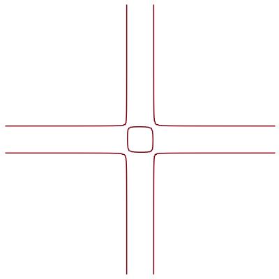
Figure 1. The set of real zeros in $\mathrm{R}^{2}$ of $P_{\varepsilon}=(X_{1}^{2}-1)(X_{2}^{2}-1)-{\varepsilon}$ for small ${\varepsilon}$.

Proposition 10.

Let $B_{1},\ldots,B_{\ell}\subset\mbox{$\mathbb{R}$}^{k},1\leq\ell\leq k$, and for $1\leq i\leq\ell$, $B_{i}=[0,d_{i,1}]\ \times\cdots\times[0,d_{i,k}]$. We denote by $\mathbf{d}=\left(d_{i,j}\right)_{\begin{subarray}{c}1\leq i\leq\ell\\ 1\leq j\leq k\end{subarray}}$. Let $\mathcal{P}=\{P_{1},\ldots,P_{\ell}\}\subset\mathrm{C}[X_{1},\ldots,X_{k}$, with $\mathrm{supp}(P_{i})=B_{i}$, $V_{\mathrm{C}}=\mathrm{Zer}(\mathcal{P},\mathrm{C}^{k})$, with $\mathcal{P}$ assumed to be generic.

(3.28) $$b(V_{\mathrm{C}},\mathbb{Z}_{2}) \leq 1+(-1)^{k-\ell+1}+\sum_{j=\ell}^{k}\sum_{J\in\binom{[1,k]}{j}}(-1)^{k-j}\sum_{\begin{subarray}{c}\bm{\alpha}=(\alpha_{1},\ldots,\alpha_{\ell})\in\mathbb{Z}_{>0}^{\ell}\\ \alpha_{1}+\cdots+\alpha_{\ell}=j\end{subarray}}N(\mathbf{d}_{J},\bm{\alpha})$$

$$\leq O(\ell)^{k}\cdot\max_{\begin{subarray}{c}\bm{\alpha}=(\alpha_{1},\ldots,\alpha_{\ell})\in\mathbb{Z}_{>0}\\ \alpha_{1}+\cdots+\alpha_{\ell}=k\end{subarray}}\max_{(J_{1},\ldots,J_{\ell})\in\binom{[1,k]}{\bm{\alpha}}}\left(\prod_{\begin{subarray}{c}1\leq i\leq\ell\\ j\in J_{i}\end{subarray}}d_{i,j}\right),$$

where for $J\subset[1,k]$, $\mathbf{d}_{J}$ is the $\ell\times\mathrm{card}(J)$ sub-matrix obtained by extracting the columns corresponding to $J$ in $\mathbf{d}$, and $N(\mathbf{d}_{J},\bm{\alpha})$ is defined in (3.5).

The same bound as in (3.28) also hold for $b(\mathrm{Zer}(\mathcal{P},\mathrm{R}^{k}),\mathbb{Z}_{2})$, if additionally $\mathcal{P}$ has coefficients in $\mathrm{R}$.

Proof.

See §8.2 in the Appendix. ∎

3.5.1. Quadratic and partially quadratic case

We now use Theorem 24 to obtain bounds on the Betti numbers of generic intersections of quadratic and partially quadratic polynomials. Since the dependence of the bounds on the different parameters in this case are rather different from the previous cases, we start by explaining the most simple case in detail.

Proposition 11.

Let $P_{1},P_{2}$ be two generic quadratic polynomials in $\mathrm{C}[X_{1},\ldots,X_{k}]$. Then,

(3.29) $$b(\mathrm{Zer}(\{P_{1},P_{2}\},\mathrm{C}^{k}),\mathbb{Z}_{2}) = 2k.$$

Proof.

First note that $\mathrm{supp}(P_{1}),\mathrm{supp}(P_{2})$ are both equal to the convex hull of $\mathbf{0},(2,0,\ldots,0),\ldots,(0,\ldots,0,2)$. It follows applying Theorem 24 that for $k\geq 2$,

$$\chi(\mathrm{Zer}(\{P_{1},P_{2}\},\mathrm{C}^{k}),\mathbb{Z}_{2}) = \sum_{j=2}^{k}\binom{k}{j}(-1)^{j}(j-1)j!\frac{2^{j}}{j!}$$

$$= 1+\sum_{j=0}^{k}\binom{k}{j}(-1)^{j}(j-1){2^{j}}$$

$$= 1+\sum_{j=0}^{k}\binom{k}{j}(-1)^{j}j2^{j}-\sum_{j=0}^{k}\binom{k}{j}(-1)^{j}2^{j}$$

$$= 1+2\sum_{j=0}^{k}\binom{k}{j}(-1)^{j}j2^{j-1}-\sum_{j=0}^{k}\binom{k}{j}(-1)^{j}2^{j}$$

$$= 1+2k(1-2)^{k-1}(-1)-(1-2)^{k}$$

$$= 1+(-1)^{k}2k-(-1)^{k}$$

$$= 1+(-1)^{k}(2k-1).$$

This implies (using Eqn. (3.11)) that

$$b(V,\mathbb{Z}_{2}) = 1+(-1)^{k}(\chi(V_{k},\mathbb{Z}_{2})-1)$$

$$= 1+(-1)^{k+1}+(-1)^{k}\chi(V_{k},\mathbb{Z}_{2})$$

$$= 1+(-1)^{k+1}+(-1)^{k}\left(1+(-1)^{k}(2k-1)\right)$$

$$= 2k.$$

∎

Remark 22.

In particular, when $k=2$, $b(\mathrm{Zer}(\{P_{1},P_{2}\},\mathrm{C}^{k}),\mathbb{Z}_{2})=4$, agreeing with the fact that two generic quadratic polynomials in two variables will have $4$ points in their intersection.

In the case $k=3$, notice that intersection, $W$ of two generic quadric surfaces in $\mathbb{P}_{\mathrm{C}}^{3}$ is topologically a torus $\mathbf{S}^{1}\times\mathbf{S}^{1}$. The intersection of $W$ with the plane at infinity is $4$ points. Hence, $\mathrm{Zer}(\{P_{1},P_{2}\},\mathrm{C}^{k})$ in this case is homeomorphic to $\mathbf{S}^{1}\times\mathbf{S}^{1}$ minus $4$ points. This gives,

$$b_{0}(\mathrm{Zer}(\{P_{1},P_{2}\},\mathrm{C}^{k}),\mathbb{Z}_{2}) = 1,$$

$$b_{1}(\mathrm{Zer}(\{P_{1},P_{2}\},\mathrm{C}^{k}),\mathbb{Z}_{2}) = 5.$$

This gives, $\chi(V,\mathbb{Z}_{2})=-4$ which agrees with the formula above.

We now consider a more general situation.

Proposition 12.

Let $\mathcal{P}=\{P_{1},\ldots,P_{\ell}\}$ be a finite set of generic polynomials in $\mathrm{C}[X_{1},\ldots,X_{k_{1}},Y_{1},\ldots,Y_{k_{2}}]$ with $0<\ell\leq k=k_{1}+k_{2}$, and $\deg_{\mathbf{X}}(P_{i})\leq d,\deg_{\mathbf{Y}}(P_{i})\leq 2$.

Then,

(3.30) $$b(\mathrm{Zer}(\mathcal{P},\mathrm{C}^{k}),\mathbb{Z}_{2})\leq 2+(-1)^{k-\ell+1}+\ell 2^{\ell}(k_{1}+k_{2})^{\ell-1}\left(2d(k_{1}+k_{2})+1\right)^{k_{1}}.$$

The same bound as in (3.30) also holds for $b(\mathrm{Zer}(\mathcal{P},\mathrm{R}^{k}),\mathbb{Z}_{2})$, if additionally $\mathcal{P}$ has coefficients in $\mathrm{R}$.

Proof.

See §8.2 in the Appendix. ∎

3.5.2. Generic intersections of quadrics in affine and projective spaces

Since the intersections of quadrics is a very well studied topic [3, 36] we investigate the special case of Proposition 12 where $k_{1}=0$. In particular, we calculate the leading coefficient of the polynomial in $k$ giving the sum of the Betti numbers of the intersection of $\ell$ generic quadrics in $\mathbb{P}_{\mathrm{C}}^{k}$ for every fixed $\ell$, thus solving a problem posed in [36] (see Eqn. 3.33 below).

Setting $k_{1}=0$ and $k_{2}=k$, in the above calculation and keeping the same notation, we obtain that

(3.31) $$\chi(\mathrm{Zer}(\mathcal{P},\mathrm{C}^{k}),\mathbb{Z}_{2}) = 1+(-1)^{k+1}\left(\sum_{h=0}^{\ell-1}\binom{k}{h}(-2)^{h}\right).$$

In order to calculate the Euler-Poincaré characteristic of a generic complete intersection of dimension $k-\ell$ in $\mathbb{P}_{\mathrm{C}}^{k}$ in terms of a fixed degree sequence $(d_{1},\ldots,d_{\ell})$, it suffices to take the sum of the Euler-Poincaré characteristics of the corresponding affine varieties in $\mathrm{C}^{k},\mathrm{C}^{k-1},\ldots,\mathrm{C}^{\ell}$ (with the same degree sequence). Applying this in our situation we obtain that if $\mathcal{P}=\{P_{1},\ldots,P_{\ell}\}$ are generic homogeneous quadrics in $\mathrm{C}[X_{0},\ldots,X_{k}]$ then it follows from the above and (3.31) that

(3.32) $$\chi(\mathrm{Zer}(\mathcal{P},\mathbb{P}_{\mathrm{C}}^{k}),\mathbb{Z}_{2}) = \sum_{j=\ell}^{k}\left(1+(-1)^{j+1}\left(\sum_{h=0}^{\ell-1}\binom{j}{h}(-2)^{h}\right)\right)$$

$$= \sum_{h=0}^{\ell-1}(-2)^{h}\left(\sum_{j=\ell}^{k}(-1)^{j+1}\binom{j}{h}\right)+(k-\ell+1),$$

and using Proposition 4

(3.33) $$b(\mathrm{Zer}(\mathcal{P},\mathbb{P}_{\mathrm{C}}^{k}),\mathbb{Z}_{2})=(1+(-1)^{k-\ell+1})(k-\ell+1)+(-1)^{k-\ell}\chi(\mathrm{Zer}(\mathcal{P},\mathbb{P}_{\mathrm{C}}^{k}),\mathbb{Z}_{2}),$$

for $\ell<k$.

It is easy to deduce directly from (3.32) and (3.33) that for $\ell\geq 3$

(3.34) $$b(\mathrm{Zer}(\mathcal{P},\mathbb{P}_{\mathrm{C}}^{k}),\mathbb{Z}_{2}) = \frac{2^{\ell-2}}{(\ell-1)!}{k}^{\ell-1}+O(k^{\ell-2}),$$

for fixed $\ell$ and $k$ large.

To see this define,

$$B(h,k,\ell)=2^{h}\left(\sum_{j=\ell}^{k}(-1)^{j+1}\binom{j}{h}\right).$$

$B(\ell-1,k,\ell)$ is the absolute value of the term corresponding to $h=\ell-1$ in the expression in (3.32). We have

(3.35) $$B(\ell-1,k,\ell) = 2^{\ell-1}\left(\binom{k}{\ell-1}-\binom{k-1}{\ell-1}+\cdots+(-1)^{k-\ell-1}\binom{\ell-1}{\ell-1}\right)$$

$$= 2^{\ell-1}\left(\binom{k-1}{\ell-2}+\binom{k-3}{\ell-2}+\cdots\right).$$

Lemma 2.

For $p\geq 0$, and all large $n$,

$$\sum_{i=0}^{\lfloor(n-p)/2\rfloor}\binom{n-2i}{p} = \frac{1}{2}\binom{n+1}{p+1}+O(n^{p}).$$

Proof.

Let

$$A(n,p)=\sum_{i=0}^{\lfloor(n-p)/2\rfloor}\binom{n-2i}{p}.$$

From standard binomial identities we deduce

$$A(n,p)+A(n-1,p)=\sum_{i=0}^{\lfloor(n-p)\rfloor}\binom{n-i}{p}=\binom{n+1}{p+1},$$

and

$$A(n,p)-A(n-1,p)=A(n-1,p-1)\leq A(n,p-1).$$

The lemma now follows by induction on $p$, the case $p=0$ being trivial. ∎

It follows from Lemma 2 and (3.35) that

(3.36) $$B(\ell-1,k,\ell) = 2^{\ell-2}\binom{k}{\ell-1}+O(k^{\ell-2}).$$

Moreover,

(3.37) $$\sum_{h=0}^{\ell-2}B(h,k,\ell) = O(k^{\ell-2}).$$

It follows from (3.36), (3.37), Proposition 4 that

(3.38) $$b(\mathrm{Zer}(\mathcal{P},\mathbb{P}_{\mathrm{C}}^{k}),\mathbb{Z}_{2}) = 2^{\ell-2}\binom{k}{\ell-1}+O(k^{\ell-2}),$$

which implies inequality (3.34).

This answers a question raised in [36, page 4], where the first few values of the leading coefficients were given, and the problem of calculating it exactly was posed. Notice that this coefficient, $\frac{2^{\ell-2}}{(\ell-1)!}$, goes to zero exponentially fast with $\ell$.

Using Theorem 22 (Smith inequality) and (3.34) we obtain the following theorem (cf. [36]).

Theorem 25.

Let $\mathcal{P}\subset\mathrm{R}[X_{0},\ldots,X_{k}]$ be a set of $\ell$ generic homogeneous polynomials of degree $2$. Then for every fixed $\ell\geq 3$,

$$b(\mathrm{Zer}(\mathcal{P},\mathbb{P}_{\mathrm{R}}^{k}),\mathbb{Z}_{2}) \leq 2^{\ell-2}\binom{k}{\ell-1}+O(k^{\ell-2}).$$

Remark 23.

Note that a more naive approach using a bound of $(O(k))^{\ell-1}$ on the Betti numbers of generic intersections of $\ell$ affine quadrics in $\mathrm{C}^{k}$, the fact that $\mathbb{P}_{\mathrm{C}}^{k}$ is the disjoint union of $\mathrm{C}^{k},\mathrm{C}^{k-1},\ldots,\mathrm{C}^{0}$, and the additivity property of the Euler-Poincaré characteristics, yields a slightly coarser bound of $(O(k))^{\ell}$. The signs thus play an important role in the proof of Theorem 25. Finally, note that the more general version of Theorem 25, with a slightly worse bound but without any assumption of genericity appears in Theorem 17.

3.5.3. One quadratic block and multi-degree case

We now consider the case of generic intersections of polynomials having one block of variables of degree $2$, while the other variables are allowed to have different degrees. More precisely, we prove:

Proposition 13.

Let $\mathcal{P}=\{P_{1},\ldots,P_{\ell}\}\subset\mathrm{C}[X_{1},\ldots,X_{k_{1}},Y_{1},\ldots,Y_{k_{2}}]$ be a finite set of generic polynomials with $\deg_{X_{i}}(P)\leq d_{i}$ and $\deg_{\mathbf{Y}}(P)\leq 2$ for all $P\in\mathcal{P}$ with $d_{1}\geq d_{2}\geq\cdots\geq d_{k_{1}}$ and $0<\ell\leq k=k_{1}+k_{2}$. Then,

(3.39) $$b(\mathrm{Zer}(\mathcal{P},\mathrm{C}^{k}),\mathbb{Z}_{2})\leq 2+(-1)^{k-\ell+1}+\ell 2^{\ell}k_{1}!(k_{1}+k_{2})^{\ell-1}\left(2(k_{1}+k_{2})+1\right)^{k_{1}}d_{1}\cdots d_{k_{1}}.$$

The same bound as in (3.30) holds for $b(\mathrm{Zer}(\mathcal{P},\mathrm{R}^{k}),\mathbb{Z}_{2})$, if additionally $\mathcal{P}$ has coefficients in $\mathrm{R}$.

Proof.

See §8.2 in the Appendix. ∎

4. Proofs of the main theorems

4.1. Summary of the methods

Our main tools are the bounds on the Betti numbers of generic intersections proved in §3.5 above, which are all consequences of Theorem 24 and Theorem 22 (Smith inequality), the techniques of infinitesimal perturbations ([17, Chapter 7]), and the inequalities derived from the Mayer-Vietoris exact sequence (Proposition 1). Using the techniques of infinitesimal perturbations, and the inequalities in Proposition 1, we reduce the problem of bounding the Betti numbers of semi-algebraic sets defined by general (non-generic) polynomials $P\in\mathcal{P}\subset\mathrm{R}[X_{1},\ldots,X_{k}]$ with support contained in given Newton polytopes $\Delta_{P},P\in\mathcal{P}$ (the tuple $(\Delta_{P})_{P\in\mathcal{P}}$ satisfying Property 1), to bounding the Betti numbers of a collection of real affine algebraic varieties defined by generic polynomials with (nearly) the same support. The proofs of Theorems 11, 12, 14, 16, and 20 (i.e. the cases of different classes of algebraic sets) are very similar to each other, differing only in the application of the appropriate generic bounds. Because of this reason we explain only the proof of Theorem 11 in full detail. Similarly, the proofs of Theorems 13, 15, 18, and 21 (the semi-algebraic cases) are all similar in structure to the proof of [17, Theorem 7.30] and [17, Theorem 7.38], again differing only in the application of the appropriate generic bounds. We refer the reader to [17] for any missing detail.

4.2. Deformation to generic

As mentioned above we will reduce the problem of bounding the Betti numbers of semi-algebraic sets defined by general (non-generic) polynomials $P\in\mathcal{P}\subset\mathrm{R}[X_{1},\ldots,X_{k}]$ to bounding the Betti numbers of a collection of real affine algebraic varieties defined by generic polynomials with the same support. For this we will need to following technical lemma.

Lemma 3.

Let $V\subset\mathrm{R}^{N}$ be a Zariski closed subset with $\dim_{\mathrm{R}}(V)<N$. Let $\mathbf{a}\in\mathrm{R}^{N}\setminus V$. Then, for all $\mathbf{b}\in\mathrm{R}^{N}$, $(1-\delta)\cdot\mathbf{b}+\delta\cdot\mathbf{a}\not\in\mathrm{Ext}(V,\mathrm{R}{\langle}\delta{\rangle})$.

Proof.

Since, $V$ is Zariski-closed, $V=\mathrm{Zer}(P,\mathrm{R}^{N})$ for some $P\in R[X_{1},\ldots,X_{N}]$. The polynomial $F(T):=P((1-T)\mathbf{b}+T\mathbf{a})\in\mathrm{R}[T]$ is not identically $0$, since $F(1)\neq 0$. Hence, there exists $t_{0}\in\mathrm{R}$ with $t_{0}>0$, such that $F$ does not vanish in the interval $(0,t_{0})$. This implies that $P((1-\delta)\cdot\mathbf{b}+\delta\cdot\mathbf{a})\neq 0$, and hence $(1-\delta)\cdot\mathbf{b}+\delta\cdot\mathbf{a}\not\in\mathrm{Ext}(V,\mathrm{R}{\langle}\delta{\rangle})$. ∎

Corollary 2.

For $1\leq i\leq\ell$, let $\Delta_{i}\subset\mathbb{Q}^{k}$ be a convex polytope, and let $H_{i}=\sum_{\boldsymbol{\alpha}\in\Delta_{i}\cap\mathbb{N}^{k}}a_{i,\boldsymbol{\alpha}}\mathbf{X}^{\boldsymbol{\alpha}},P_{i}=\sum_{\boldsymbol{\alpha}\in\Delta_{i}\cap\mathbb{N}^{k}}b_{i,\boldsymbol{\alpha}}\mathbf{X}^{\boldsymbol{\alpha}},\in\mathrm{R}[X_{1},\ldots,X_{k}],1\leq i\leq\ell$. Let $V\subset\mathrm{R}^{N}$ be a real variety, with $N=\sum_{i=1}^{\ell}\mathrm{card}(\Delta_{i}\cap\mathbb{N}^{k})$. Let $\mathbf{a}=(\ldots,a_{i,\boldsymbol{\alpha}},\ldots),\mathbf{b}=(\ldots,b_{i,\boldsymbol{\alpha}},\ldots)\in\mathrm{R}^{N}$ denote the vectors of coefficients of $(H_{1},\ldots,H_{\ell})$ and $(P_{1},\ldots,P_{\ell})$ respectively. Suppose also that $\mathbf{a}\not\in V$. Then, if $\mathbf{c}\in\mathrm{R}{\langle}\delta{\rangle}^{N}$ is the vector of coeffcients of $(1-\delta)\cdot P_{1}+\delta\cdot H_{1},\ldots,(1-\delta)\cdot P_{\ell}+\delta\cdot H_{\ell}$, then $\mathbf{c}\not\in\mathrm{Ext}(V,\mathrm{R}{\langle}\delta{\rangle})$. (In other words, using the language introduced in Definition 1, if $(H_{1},\ldots,H_{\ell})$ is a generic tuple of polynomials, so is $(1-\delta)\cdot P_{1}+\delta\cdot H_{1},\ldots,(1-\delta)\cdot P_{\ell}+\delta\cdot H_{\ell}$ for all tuples of polynomials $(P_{1},\ldots,P_{\ell})$ with $\mathrm{supp}(P_{i})\subset\Delta_{i},1\leq i\leq\ell$.)

Proof.

Apply Lemma 3. ∎

4.3. Proof of Theorem 11

Proof of Theorem 11.

We first prove

(4.1) $$b(V,\mathbb{Z}_{2})\leq\frac{1}{2}(1+(2d-1)^{k}).$$

Let $r>0$, and let

$$F(X_{1},\ldots,X_{k})=(Q_{1}^{2}+\cdots+Q_{\ell}^{2})/(r^{2}-\|\mathbf{X}\|^{2}).$$

The set of critical values of $F$ is finite, so there exists $c_{0}\in\mathrm{R},c_{0}>0$ so that $\mathrm{Zer}(\tilde{Q},\mathrm{R}^{k})$ is a non-singular hypersurface in $\mathrm{R}^{k}$, where

(4.2) $$\tilde{Q}_{r}=Q_{1}^{2}+\cdots+Q_{\ell}^{2}+c(\|\mathbf{X}\|^{2}-r^{2})=0,$$

for all $c\in(0,c_{0})$.

Denote by $\tilde{V}=\mathrm{Zer}(\tilde{Q},\mathrm{R}^{k})$. Since $\deg(\tilde{Q})\leq 2d$, we have by Proposition 6 that

(4.3) $$b(\tilde{V}_{r},\mathbb{Z}_{2})\leq 1+(2d-1)^{k}.$$

Notice that the the closed and bounded semi-algebraic set, $S_{r}$ defined by $\tilde{Q}_{r}\leq 0$, is semi-algebraically homotopy equivalent to $V_{r}=V\cap\overline{B_{k}(0,r)}$.

Since $S_{r}$ is bounded by $\tilde{V}_{r}$,

(4.4) $$b(S_{r},\mathbb{Z}_{2})\leq\frac{1}{2}b(\tilde{V}_{r},\mathbb{Z}_{2})$$

(using for example [17, Proposition 7.27]).

Combining (4.3) and (4.4) we obtain

$$b(V_{r},\mathbb{Z}_{2})=b(S_{r},\mathbb{Z}_{2})\leq\frac{1}{2}b(\tilde{V}_{r},\mathbb{Z}_{2})\leq\frac{1}{2}(1+(2d-1)^{k}),$$

which proves (4.1).

Finally, using conical structure theroem at infinity for semi-algebraic sets, we have that for all $r$ large enough, $V_{r}$ is semi-algebraically homeomorphic to $V$, from whence it follows that

$$b(V,\mathbb{Z}_{2})\leq\frac{1}{2}b(\tilde{V}_{r},\mathbb{Z}_{2})\leq\frac{1}{2}(1+(2d-1)^{k}).$$

We now prove that

(4.5) $$b(V,\mathbb{Z}_{2})\leq\binom{\ell}{k}2^{k}d^{\prime k}+\sum_{j=1}^{k-1}\binom{\ell}{j}2^{j}(F_{1}(d^{\prime},k,j)+F_{2}(d^{\prime},k,j))+3,$$

where $d^{\prime}$ is the least even integer $\geq 0$.

Denote for every even $d^{\prime\prime}\geq 0$, by $H_{d^{\prime\prime},k}\subset\mathrm{R}{\langle}{\varepsilon}{\rangle}[X_{1},\ldots,X_{k}]$ the subspace of polynomials of degree $\leq d^{\prime\prime}$, and observe that there is a non-empty, open semi-algebraic subset $U_{d^{\prime\prime},k}\subset H_{d^{\prime\prime},k}$ such that for every $H\in U_{d^{\prime\prime},k}$, $H$ is strictly positive on $\mathrm{R}{\langle}{\varepsilon}_{0}{\rangle}^{k}$.

Denote by $W\subset H_{2,k}\times\underbrace{H_{d^{\prime\prime},k}\times\cdots\times H_{d^{\prime\prime},k}}_{2\ell}$ the non-empty Zariski open subset of generic tuples of polynomials (cf. Definition 1). Then, $W\cap U_{2,k}\times U_{d^{\prime},k}\times\cdots\times U_{d^{\prime},k}$ is clearly non-empty. Choose polynomials $H_{0},H_{1},\ldots,H_{2\ell}$ such that the tuple $(H_{0},H_{1},\ldots,H_{2\ell})\in W\cap U_{2,k}\times U_{d^{\prime},k}\times\cdots\times U_{d^{\prime},k}$.

Let

$$\tilde{Q}_{0}=(1-\delta)\cdot(\|\mathbf{X}\|^{2}-1/{\varepsilon}^{2})-\delta\cdot H_{0},$$

and for $1\leq i\leq\ell$, let

$$\tilde{Q}_{i,+} = (1-\delta)\cdot Q_{i}+\delta\cdot H_{2i-1},$$

$$\tilde{Q}_{i,-} = (1-\delta)\cdot Q_{i}-\delta\cdot H_{2i}.$$

Also, let $\mathrm{R}^{\prime}=\mathrm{R}{\langle}{\varepsilon},\delta{\rangle}$.

Note that using Corollary 2, the polynomials $Q_{0},Q_{1,\pm},\ldots,Q_{\ell,\pm}$ are generic.

We need the following lemma.

Lemma 4.

The real algebraic variety $\mathrm{Ext}(V,\mathrm{R}^{\prime})$ (cf. Notation 9) is semi-algebraically homotopy equivalent to the semi-algebraic set $\tilde{S}\subset\mathrm{R}^{\prime k}$ defined by

$$(\tilde{Q}_{0}<0)\wedge\bigwedge_{1\leq i\leq\ell}((\tilde{Q}_{i,+}>0)\wedge(\tilde{Q}_{i,-}<0)).$$

Proof.

Follows from [17, Lemma 16.17]. ∎

Let

$$\tilde{W}=\mathrm{Zer}(\tilde{Q}_{0},\mathrm{R}^{\prime k})\cup\bigcup_{\begin{subarray}{c}1\leq i\leq\ell\\ \sigma\in\{+,-\}\end{subarray}}\mathrm{Zer}(\tilde{Q}_{i,\sigma},\mathrm{R}^{\prime k}).$$

Note that $\mathrm{R}^{\prime k}\setminus\tilde{W}$ is an open semi-algebraic set, and $\tilde{S}$ is the union of a subset of the semi-algebraically connected components of $\mathrm{R}^{\prime k}\setminus\tilde{W}$ which are bounded. This implies that

$$b(\tilde{S},\mathbb{Z}_{2})\leq b(\overset{\circ}{\mathrm{R}^{\prime k}}\setminus\tilde{W},\mathbb{Z}_{2}),$$

where $\overset{\circ}{\mathrm{R}^{\prime k}}$ is the one-point compactification of $\mathrm{R}^{\prime k}$, and is semi-algebraically homeomorphic to the sphere $\mbox{${\bf S}$}^{k}$ defined over $\mathrm{R}^{\prime}$. We will now use Alexander duality theorem for semi-algebraic subsets defined over $\mathrm{R}^{\prime}$. Note that the statement of this theorem over $\mathbb{R}$ restricted to semi-algebraic sets (proved for example in [43, page 296]) implies the corresponding statement over $\mathrm{R}^{\prime}$ by a standard application of the Tarski-Seidenberg transfer principle. Using Alexander duality and the fact that $\tilde{W}$ is non-empty we obtain

$$b(\tilde{S},\mathbb{Z}_{2})\leq b(\overset{\circ}{\mathrm{R}^{\prime k}}\setminus\tilde{W},\mathbb{Z}_{2})\leq b(\tilde{W},\mathbb{Z}_{2})+1.$$

We now bound $b(\tilde{W},\mathbb{Z}_{2})$ using Proposition 1 noting that $\tilde{W}$ is the union of $2\ell+1$ real algebraic sets.

Let

$$\tilde{\mathcal{Q}}=\{\tilde{Q}_{i,\sigma}\;\mid\;1\leq i\leq\ell,\sigma\in\{+,-\}\}.$$

Proposition 1 implies that

(4.6) $$b(\tilde{W},\mathbb{Z}_{2})\leq\sum_{\begin{subarray}{c}\tilde{\mathcal{Q}}^{\prime}\subset\tilde{\mathcal{Q}},\\ \mathrm{card}(\tilde{\mathcal{Q}}^{\prime})\leq k-1\end{subarray}}b(\mathrm{Zer}(\{\tilde{Q}_{0}\}\cup\tilde{\mathcal{Q}}^{\prime},\mathrm{R}^{\prime k}),\mathbb{Z}_{2})+\sum_{\begin{subarray}{c}\tilde{\mathcal{Q}}^{\prime}\subset\tilde{\mathcal{Q}},\\ \mathrm{card}(\tilde{\mathcal{Q}}^{\prime})\leq k\end{subarray}}b(\mathrm{Zer}(\tilde{\mathcal{Q}}^{\prime},\mathrm{R}^{\prime k}),\mathbb{Z}_{2}).$$

Notice that for $\tilde{\mathcal{Q}}^{\prime}\subset\tilde{\mathcal{Q}}$ with $\mathrm{card}(\tilde{\mathcal{Q}}^{\prime})=k$, we have by Bezout’s theorem that

(4.7) $$b(\mathrm{Zer}(\tilde{\mathcal{Q}}^{\prime},\mathrm{R}^{\prime k}),\mathbb{Z}_{2})\leq d^{\prime k}.$$

Inequalities (4.7) and (4.6) imply

(4.8) $$b(\tilde{W},\mathbb{Z}_{2})\leq\binom{\ell}{k}2^{k}d^{\prime k}+\sum_{\begin{subarray}{c}\tilde{\mathcal{Q}}^{\prime}\subset\tilde{\mathcal{Q}},\\ \mathrm{card}(\tilde{\mathcal{Q}}^{\prime})\leq k-1\end{subarray}}(b(\mathrm{Zer}(\{\tilde{Q}_{0}\}\cup\tilde{\mathcal{Q}}^{\prime},\mathrm{R}^{\prime k}),\mathbb{Z}_{2})+b(\mathrm{Zer}(\tilde{\mathcal{Q}}^{\prime},\mathrm{R}^{\prime k}),\mathbb{Z}_{2})).$$

Finally for $\tilde{\mathcal{Q}}^{\prime}\subset\tilde{\mathcal{Q}}$ with $\mathrm{card}(\tilde{\mathcal{Q}}^{\prime})=j,1\leq j\leq\min(\ell,k-1)$, we have,

(4.9) $$b(\mathrm{Zer}(\{\tilde{Q}\}\cup\tilde{\mathcal{Q}}^{\prime},\mathrm{R}^{\prime k}),\mathbb{Z}_{2})\leq F_{1}(d^{\prime},k,j),$$

using inequality (19) in Remark 19, and

(4.10) $$b(\mathrm{Zer}(\tilde{\mathcal{Q}}^{\prime},\mathrm{R}^{\prime k}),\mathbb{Z}_{2}))\leq F_{2}(d^{\prime},k,j)$$

using inequality (3.21) in Proposition 7. Note that if $j=0$, then

$$b(\mathrm{Zer}(\{\tilde{Q_{0}}\},\mathrm{R}^{\prime k}),\mathbb{Z}_{2})=2,$$

and

$$b(\mathrm{Zer}(\tilde{\mathcal{Q}}^{\prime},\mathrm{R}^{\prime k}),\mathbb{Z}_{2})=b(\mathrm{Zer}(\emptyset,\mathrm{R}^{\prime k}),\mathbb{Z}_{2})=b(\mathrm{R}^{\prime k},\mathbb{Z}_{2})=1.$$

Inequality (4.5) now follows from Lemma 4, and inequalities (4.6), (4.8), (4.9), and (4.10).

Finally, inequality (2.1) follows from inequalities (4.1) and (4.5). ∎

4.4. Proofs of Theorems 12 and 13

Proof of Theorem 12.

We first prove

(4.11) $$b(V,\mathbb{Z}_{2}) \leq \frac{1}{2}G_{\mathrm{gen}}(2\mathbf{d},\mathbf{k},1).$$

The proof is similar to that of Theorem 11, but we note that the polynomial (4.2) $\tilde{Q}=Q_{1}^{2}+\cdots+Q_{\ell}^{2}+c(\|\mathbf{X}\|^{2}-r^{2})\in\mathrm{R}[\mathbf{X}^{(1)},\ldots,\mathbf{X}^{(p)}]$ has multi-degree bounded by $2\mathbf{d}$. Therefore, $b(\mathrm{Zer}(\tilde{Q},\mathrm{R}^{k}),\mathbb{Z}_{2})\leq G_{\mathrm{gen}}(2\mathbf{d},\mathbf{k},1)$ using Proposition 8.

We now prove

(4.12) $$b(V,\mathbb{Z}_{2}) \leq 3+\sum_{j=1}^{k}\binom{\ell}{j}2^{j}(G_{\mathrm{gen}}(\mathbf{d}^{\prime},\mathbf{k},j)+G_{\mathrm{gen}}(\mathbf{d}^{\prime},\mathbf{k},j+1)).$$

We proceed in the same manner as in the proof of Theorem 11. We note that the sphere can also be viewed as a polynomial in $\mathrm{R}[\mathbf{X}^{(1)},\ldots,\mathbf{X}^{(p)}]$, where each block has degree equal to $2$. Notice that we assume all $d_{i}\geq 2$, so we can view the polynomial $Q_{0}$ in the proof of Theorem 11 as another polynomial with the same block structure and degree bounds as each polynomial in $\mathcal{Q}$. Therefore, we can replace both $F_{1}(d^{\prime},k,j)$ (resp. $F_{2}(d^{\prime},k,j)$) with $G_{\mathrm{gen}}(\mathbf{d}^{\prime},\mathbf{k},j+1)$ (resp. $G_{\mathrm{gen}}(\mathbf{d}^{\prime},\mathbf{k},j)$). The theorem follows from inequalities (4.11) and (4.12). ∎

Proof of Theorem 13.

The proof is similar to those of [17, Theorem 7.30] and [17, Theorem 7.38] with the following modification that instead of using Theorem 1 for bounding the sum of the Betti numbers of various algebraic sets that occur, we use the bound in Theorem 12. ∎

4.5. Proofs of Theorems 14 and 15

Proof of Theorem 14.

The proof is similar to the proof of Theorem 12 using Proposition 10 instead of Proposition 8. ∎

Proof of Theorem 15.

The proof is similar to the proof of Theorem 13 using Theorem 14 instead of Theorem 12. ∎

4.6. Proofs of Theorems 16, 17, 18, and 19

Proof of Theorem 16.

The proof is similar to that of Theorem 12. Since we have $\ell$ partially quadratic polynomials, we use $H_{\mathrm{gen}}(d^{\prime},k_{1},k_{2},j)$ in place of $G_{\mathrm{gen}}(\mathbf{d}^{\prime},\mathbf{k},j)$, where $H_{\mathrm{gen}}(d^{\prime},k_{1},k_{2},j)$ is the bound from Proposition 12, noting that we assume $d\geq 2$. ∎

Proof of Theorem 17.

The proof is similar to the proof of Theorem 11 above using generic positive quadrics to perturb the given polynomials (in lieu of the polynomials $H_{i}$ in the proof of Theorem 11). More precisely, for $1\leq i\leq\ell$, let

$$\tilde{Q}_{i,+} = (1-\delta)\cdot Q_{i}+\delta\cdot H_{2i-1},$$

$$\tilde{Q}_{i,-} = (1-\delta)\cdot Q_{i}-\delta\cdot H_{2i}.$$

where the polynomials $H_{1},\ldots,H_{2\ell}$ are chosen to be generic positive quadrics. Using Corollary 2, the polynomials $Q_{0},Q_{1,\pm},\ldots,Q_{\ell,\pm}$ are generic.

Also, let $\mathrm{R}^{\prime}=\mathrm{R}{\langle}\delta{\rangle}$.

Using Lemma 4 The real algebraic variety $\mathrm{Ext}(V,\mathrm{R}^{\prime})$ (cf. Notation 9) is semi-algebraically homotopy equivalent to the semi-algebraic set $\tilde{S}\subset\mathbb{P}_{\mathrm{R}^{\prime}}^{k}$ defined by

$$\bigwedge_{1\leq i\leq\ell}((\tilde{Q}_{i,+}>0)\wedge(\tilde{Q}_{i,-}<0)).$$

Let

$$\tilde{W}=\bigcup_{\begin{subarray}{c}1\leq i\leq\ell\\ \sigma\in\{+,-\}\end{subarray}}\mathrm{Zer}(\tilde{Q}_{i,\sigma},\mathrm{R}^{\prime k}).$$

Note that $\mathbb{P}_{\mathrm{R}^{\prime}}^{k}\setminus\tilde{W}$ is an open semi-algebraic set, and $\tilde{S}$ is the union of a subset of the semi-algebraically connected components of $\mathbb{P}_{\mathrm{R}^{\prime}}^{k}\setminus\tilde{W}$. This implies that

$$b(\tilde{S},\mathbb{Z}_{2})\leq b(\mathbb{P}_{\mathrm{R}^{\prime}}^{k}\setminus\tilde{W},\mathbb{Z}_{2}).$$

We will now use Lefschetz duality theorem for semi-algebraic subsets defined over $\mathrm{R}^{\prime}$.

Using Lefschetz duality we obtain that

(4.13) $$b(\tilde{S},\mathbb{Z}_{2}) \leq b(\mathbb{P}_{\mathrm{R}^{\prime}}^{k}\setminus\tilde{W},\mathbb{Z}_{2})$$

$$\leq b(\tilde{W},\mathbb{Z}_{2})+b(\mathbb{P}_{\mathrm{R}^{\prime}}^{k},\mathbb{Z}_{2})$$

$$= b(\tilde{W},\mathbb{Z}_{2})+k+1.$$

We now bound $b(\tilde{W},\mathbb{Z}_{2})$ using Proposition 1 noting that $\tilde{W}$ is the union of $2\ell$ real algebraic sets.

Let

$$\tilde{\mathcal{Q}}=\{\tilde{Q}_{i,\sigma}\;\mid\;1\leq i\leq\ell,\sigma\in\{+,-\}\}.$$

Proposition 1 implies that

(4.14) $$b(\tilde{W},\mathbb{Z}_{2}) \leq \sum_{\tilde{\mathcal{Q}}^{\prime}\subset\tilde{\mathcal{Q}}}b(\mathrm{Zer}(\tilde{\mathcal{Q}}^{\prime},\mathbb{P}_{\mathrm{R}^{\prime}}^{k}),\mathbb{Z}_{2}).$$

Now use inequalities (4.13), (4.14), and (3.33) to obtain the bound in the theorem. ∎

Proof of Theorem 18.

The proof is similar to those of [17, Theorem 7.30] and [17, Theorem 7.38] with the modification that instead of using Theorem 1 for bounding the sum of the Betti numbers of various algebraic sets that occur, we use the bound in Theorem 16. ∎

Proof of Theorem 19.

The proof is again similar to the proofs of Theorem 7.30 and Theorem 7.38 in [17] with several modifications. In the proof of Theorem 7.30 in [17], we let $\mathcal{Q}=\{0\}$, and $\mathcal{P}=\mathcal{P}_{1}\cup\mathcal{P}_{2}$, and we let $\mathcal{P}_{1}=\{P_{1},\ldots,P_{s}\}$ and $\mathcal{P}_{2}=\{P_{s+1},\ldots,P_{s+m}\}$. In Proposition 7.34, for each sign condition $\sigma\in\{0,1,-1\}^{\mathcal{P}}$, we redefine the basic closed semi-algebraic set

$$\overline{\mathrm{Reali}(\sigma)}\subset\mathrm{R}{\langle}\delta,\delta_{1},\ldots,\delta_{s+m},{\varepsilon}_{1},\ldots,{\varepsilon}_{s+m}{\rangle}^{k}$$

in the following way. Without loss of generality assume

$$\halign{\hbox to\displaywidth{$\hfil\displaystyle#\hfil$}\cr 0.0pt{\hfil$\displaystyle\sigma(P_{h})=0\mbox{ if }h\in I,\cr 0.0pt{\hfil$\displaystyle\sigma(P_{h})=1\mbox{ if }h\in J,\cr 0.0pt{\hfil$\displaystyle\sigma(P_{h})=-1\mbox{ if }h\in\{1,\ldots,s+m\}\setminus(I\cup J),\crcr}}}}$$

and denote by $\overline{\mathrm{Reali}(\sigma)}$ the subset of $\mathrm{R}{\langle}\delta,\delta_{1},\ldots,\delta_{s+m},{\varepsilon}_{1},\ldots,{\varepsilon}_{s+m}{\rangle}^{k}$ defined by

$$\halign{\hbox to\displaywidth{$\hfil\displaystyle#\hfil$}\cr 0.0pt{\hfil$\displaystyle\delta(|\mathbf{X}|^{2}+|\mathbf{Y}|^{2})\leq 1,\cr 0.0pt{\hfil$\displaystyle-{\varepsilon}_{h}\leq P_{h}\leq{\varepsilon}_{h},\mbox{ if }h\in I,\cr 0.0pt{\hfil$\displaystyle P_{h}\geq\delta_{h},\mbox{ if }h\in J,\cr 0.0pt{\hfil$\displaystyle P_{h}\leq-\delta_{h},\mbox{ if }h\in\{1,\ldots,s+m\}\setminus(I\cup J).\crcr}}}}}$$

It is easy to verify that Proposition 7.34 in [17] remains true with this new definition of $\overline{\mathrm{Reali}(\sigma)}$.

Now we observe that since $\mathcal{P}_{1}\subset\mathrm{R}[X_{1},\ldots,X_{k_{1}}]$, no more than $k_{1}$ polynomials amongst the set $\{P_{1}\pm\delta_{1},P_{1}\pm{\varepsilon}_{1},\ldots,P_{s}\pm\delta_{s},P_{s}\pm{\varepsilon}_{s}\}$ can have a common zero. Each non-empty real algebraic set $V$ defined by some subset of the polynomials $\{P_{1}\pm\delta_{1},P_{1}\pm{\varepsilon}_{1},\ldots,P_{s}\pm\delta_{s},P_{s}\pm{\varepsilon}_{s}\}\cup\{P_{0}\}$, where $P_{0}=\delta(|\mathbf{X}|^{2}+|\mathbf{Y}|^{2})-1$, is the set of zeros of two sets of polynomials, namely

$$\halign{\hbox to\displaywidth{$\hfil\displaystyle#\hfil$}\cr 0.0pt{\hfil$\displaystyle(P_{h}+\sigma_{h}\eta_{h})_{h\in J_{1}},\eta_{h}\in\{{\varepsilon}_{h},\delta_{h}\},\sigma_{h}\in\{\pm 1\},J_{1}\subset[1,s],\cr 0.0pt{\hfil$\displaystyle(P_{h}+\sigma_{h}\eta_{h})_{h\in J_{2}},\eta_{h}\in\{{\varepsilon}_{h},\delta_{h}\},\sigma_{h}\in\{\pm 1\},J_{2}\subset[s+1,s+m],\crcr}}}$$

and possibly $P_{0}$, with $j_{1}=\mathrm{card}(J_{1})\leq k_{1}$, and $j_{2}=\mathrm{card}(J_{2})\leq\min(m+1,k_{1}+k_{2}-j_{1}-i)$.

We also note that $V$ is defined by the $(\mathrm{card}(J_{2})+1)$ or $(\mathrm{card}(J_{2})+2)$ (depending on whether $P_{0}$ is included or not) polynomials

$$\sum_{h\in J_{1}}(P_{h}+\sigma_{h}\eta_{h})^{2},(P_{h}+\sigma_{h}\eta_{h})_{h\in J_{2}}$$

(and possibly $P_{0}$). The degrees of these polynomials are at most $2d$ in $\mathbf{X}$, and at most $2$ in $\mathbf{Y}$. We can use Theorem 16 to bound $b(V,\mathbb{Z}_{2})$ by $H(2d,k_{1},k_{2},\mathrm{card}(J_{2})+1)$ or $H(2d,k_{1},k_{2},\mathrm{card}(J_{2})+2)$ (depending on whether $P_{0}$ is included or not) (cf. Eqn. (2.6)).

Moreover, the total number of non-empty real algebraic sets $V$ that occur in the proof is bounded by

$$\sum_{\begin{subarray}{c}0\leq j_{1}\leq k_{1}\\ 0\leq j_{2}\leq\min(m+1,k_{1}+k_{2}-j_{1}-i)\end{subarray}}\binom{s}{j_{1}}\binom{m+1}{j_{2}}4^{j_{1}+j_{2}}.$$

One now obtains inequality (2.11) by following the rest of the argument in the proof of Theorem 7.30. Note that we needed to increase the number of polynomials by one by including the polynomial $P_{0}$. This accounts for the $m+1$ in the subscript of the second sum in the bound.

The proof of inequality (2.12) is by a similar modification of the proof of Theorem 7.38 in [17] and is omitted. ∎

4.7. Proofs of Theorems 20 and 21

Proof of Theorem 20.

The proof is similar to that of Theorem 12. Since we have $\ell$ partially quadratic polynomials with several blocks, we use the bound

$$M_{\mathrm{gen}}(\mathbf{d}^{\prime},k_{1},k_{2},j)$$

in place of $G_{\mathrm{gen}}(\mathbf{d}^{\prime},\mathbf{k},j)$, where $M_{\mathrm{gen}}(\mathbf{d}^{\prime},k_{1},k_{2},j)$ is the bound from Proposition 13, noting that we assume each $d_{i}\geq 2$. ∎

Proof of Theorem 21.

The proof is similar to that of Theorem 13, except that the bound for the sum of the Betti numbers corresponding to a subset of indices of cardinality $j$ is now given by $M(\mathbf{d}^{\prime},k_{1},k_{2},j)$. ∎

5. A few applications

In this section we give a few applications of the results proved in the last section.

5.1. Bounding Betti numbers of pull-backs and direct images under polynomial maps

We discuss a few immediate applications of the multi-degree bounds proved in §4.

Theorem 26 (Bound on pull-back).

Let $\mathcal{F}=\{F_{1},\ldots,F_{m}\}\subset\mathrm{R}[X_{1},\ldots,X_{k}]$ and $\mathcal{G}\subset\mathrm{R}[Y_{1},\ldots,Y_{m}]$, with $\deg(F)\leq d,F\in\mathcal{F}$, and $\deg(G)\leq D,G\in\mathcal{G}$, and let $\mathrm{card}(\mathcal{G})=s$. Let $\mathbf{F}:\mathrm{R}^{k}\rightarrow\mathrm{R}^{m}$ denote the polynomial map $x\mapsto(F_{1}(x),\ldots,F_{m}(x))$, and let $S\subset\mathrm{R}^{m}$ be a $\mathcal{G}$-closed semi-algebraic set. Then,

$$b(\mathbf{F}^{-1}(S),\mathbb{Z}_{2}) \leq \sum_{i=0}^{k+m}\sum_{j=1}^{k+m-i}\binom{m+s+1}{j}6^{j}G_{\min}(\mathbf{d},\mathbf{k},j)$$

$$\leq O(1)^{k+m}(m+s)^{k+m}d^{k}D^{m}.$$

Proof.

Suppose that $\Phi(Y_{1},\ldots,Y_{m})$ is a $\mathcal{G}$-closed formula defining $S$. Notice that $\mathbf{F}^{-1}(S)$ is semi-algebraically homeomorphic to the semi-algebraic subset of $\mathrm{R}^{k+m}$ defined by the formula

$$\Psi(\mathbf{X},\mathbf{Y}):=\bigwedge_{i=1}^{m}(Y_{i}-F_{i}=0)\wedge\Phi(Y_{1},\ldots,Y_{m}).$$

The number of polynomials appearing in $\Psi$ is bounded by $m+s$. The degrees in $\mathbf{Y}$ of the polynomials appearing in $\Psi$ are bounded by $D$, while the degrees in $\mathbf{X}$ are bounded by $d$. Applying Theorem 13 with $p=2$, $\mathbf{k}=(k,m)$, and $\mathbf{d}=(d,D)$, we obtain

$$b(\mathrm{Reali}(\Psi,\mathrm{R}^{k+m}),\mathbb{Z}_{2}) \leq \sum_{i=0}^{k+m}\sum_{j=1}^{k+m-i}\binom{m+s+1}{j}6^{j}G_{\min}(\mathbf{d},\mathbf{k},j)$$

$$\leq \sum_{i=0}^{k+m}\sum_{j=1}^{k+m-i}\binom{m+s+1}{j}6^{j}O(1)^{k+m}d^{k}D^{m}\mbox{ (using (\ref{eqn:Gmin}))}$$

$$\leq O(1)^{k+m}(m+s)^{k+m}d^{k}D^{m}.$$

∎

Theorem 27 (Bound on image).

Let $\mathcal{F}=\{F_{1},\ldots,F_{m}\},\mathcal{G}\subset\mathrm{R}[X_{1},\ldots,X_{k}]$, with $\deg(F)\leq d,F\in\mathcal{F}$, and $\deg(G)\leq D,G\in\mathcal{G}$, and let $\mathrm{card}(\mathcal{G})=s$. Let $\mathbf{F}:\mathrm{R}^{k}\rightarrow\mathrm{R}^{m}$ denote the polynomial map $x\mapsto(F_{1}(x),\ldots,F_{m}(x))$, and let $T\subset\mathrm{R}^{k}$ be a bounded $\mathcal{G}$-closed semi-algebraic set. Suppose also that $d\geq D$.

Then, for $0\leq i\leq m$,

$$b_{i}(\mathbf{F}(T),\mathbb{Z}_{2}) \leq \sum_{j=0}^{i}\sum_{h=0}^{\alpha_{j}}\sum_{\ell=1}^{\alpha_{j}-h}\binom{(j+1)(m+s)+1}{\ell}6^{\ell}G_{\min}(\mathbf{d},\mathbf{k},\ell)$$

$$\leq O(i)^{\alpha_{i}}(m+s)^{\alpha_{i}}d^{(i+1)k}D^{m}$$

where $\alpha_{i}=(i+1)k+m$.

Proof.

Using the descent spectral sequence we have that

(5.1) $$b_{i}(\mathbf{F}(T),\mathbb{Z}_{2}) \leq \sum_{j=0}^{i}b_{i-j}(\underbrace{T\times_{\mathbf{F}}\cdots\times_{\mathbf{F}}T}_{(j+1)},\mathbb{Z}_{2})$$

$$\leq \sum_{j=0}^{i}b(\underbrace{T\times_{\mathbf{F}}\cdots\times_{\mathbf{F}}T}_{(j+1)},\mathbb{Z}_{2}).$$

Suppose that $T$ is defined by a $\mathcal{G}$-closed formula $\Psi$. Notice that for all $j\geq 0$, $\underbrace{T\times_{\mathbf{F}}\cdots\times_{\mathbf{F}}T}_{(j+1)}$ is defined by the formula

$$\Psi^{(j)}(\mathbf{X}^{(0)},\ldots,\mathbf{X}^{(j)},\mathbf{Y}):=\bigwedge_{i=1}^{m}\bigwedge_{h=0}^{j}\Psi(\mathbf{X}^{(h)},\mathbf{Y})\wedge(Y_{i}-F_{i}(\mathbf{X}^{(h)})=0),$$

where $\mathbf{Y}=(Y_{1},\ldots,Y_{m}),\mathbf{X}^{(h)}=(X^{(h)}_{1},\ldots,X^{(h)}_{k}),0\leq h\leq j$.

The cardinality of the set of polynomials appearing in $\Psi^{(j)}$ is $(j+1)(m+s)$, the degree in each block $\mathbf{X}^{(h)}$ is bounded by $d$, and that in $\mathbf{Y}$ is bounded by $D$.

Denote by $\alpha_{j}=(j+1)k+m$. Now apply Theorem 13 with $p=j+2$, $\mathbf{k}=(\underbrace{k,\ldots,k}_{j+1},m)$, $\mathbf{d}=(\underbrace{d,\ldots,d}_{j+1},D)$ to obtain

(5.2) $$b(\underbrace{T\times_{\mathbf{F}}\cdots\times_{\mathbf{F}}T}_{(j+1)},\mathbb{Z}_{2}) \leq \sum_{h=0}^{\alpha_{j}}\sum_{\ell=1}^{\alpha_{j}-h}\binom{(j+1)(m+s)+1}{\ell}6^{\ell}G_{\min}(\mathbf{d},\mathbf{k},\ell)$$

$$\leq O(j)^{\alpha_{j}}(m+s)^{\alpha_{j}}d^{(j+1)k}D^{m}$$

The theorem now follows from Eqns. (5.1) and (5.2). ∎

Remark 24.

Note that versions of Theorem 26 and Theorem 27 without the distinction between the two degrees $d$ and $D$ were known before (see [26]). The novel aspect of these two theorems is the different dependence of the bounds proved on the two degrees $d,D$. In certain applications, this distinction is important.

We record the following result similar to that of Theorem 27, which is also useful in practice. The following situation occurs very frequently in semi-algebraic geometry.

Let $S_{1}\subset\mathrm{R}^{k}$, and $S_{2}\subset\mathrm{R}^{k}\times\mathrm{R}^{m}$ be semi-algebraic subsets, and $\pi_{\mathbf{X}}:\mathrm{R}^{k}\times\mathrm{R}^{m}\rightarrow\mathrm{R}^{k},\pi_{\mathbf{Y}}:\mathrm{R}^{k}\times\mathrm{R}^{m}\rightarrow\mathrm{R}^{m}$ be the two projection maps on the first and second factors resp.. Let $T=\pi_{\mathbf{Y}}(\pi_{\mathbf{X}}^{-1}(S_{1})\cap S_{2})$ (see figure below).

Theorem 28 (Set-theoretic Fourier-Mukai transform).

With the same notation as above, let $\mathcal{P}_{1}\subset\mathrm{R}[X_{1},\ldots,X_{k}]$ and $\mathcal{P}_{2}\subset\mathrm{R}[X_{1},\ldots,X_{k},Y_{1},\ldots,Y_{m}]$ be finite sets such that $S_{1}\subset\mathrm{R}^{k}$ is a $\mathcal{P}_{1}$-closed semi-algebraic set and $S_{2}\subset\mathrm{R}^{k+m}$ is a bounded $\mathcal{P}_{2}$-closed semi-algebraic set. Suppose that $\deg_{\mathbf{X}}(\mathcal{P}_{1}),\deg_{\mathbf{X}}(\mathcal{P}_{2})\leq d$ and $\deg_{\mathbf{Y}}(\mathcal{P}_{2})\leq D$. Suppose also that $d\geq D$.

Then for $0\leq i\leq m$,

$$b_{i}(T,\mathbb{Z}_{2}) \leq \sum_{j=0}^{i}\sum_{h=0}^{\alpha_{j}}\sum_{\ell=1}^{\alpha_{j}-h}\binom{(j+1)(s_{1}+s_{2})+1}{\ell}6^{\ell}G_{\min}(\mathbf{d},\mathbf{k},\ell)$$

$$\leq O(i)^{\alpha_{i}}(s_{1}+s_{2})^{\alpha_{i}}d^{(i+1)k}D^{m},$$

where $\alpha_{i}=(i+1)(k+m)+k$, and $s_{1}=\mathrm{card}(\mathcal{P}_{1}),s_{2}=\mathrm{card}(\mathcal{P}_{2})$.

Proof.

Note that the semi-algebraic set $\pi_{\mathbf{X}}^{-1}(S_{1})\cap S_{2}$ is a bounded $(\mathcal{P}_{1}\cup\mathcal{P}_{2})$-closed semi-algebraic set, with degrees in $\mathbf{X}$ bounded by $d$ and in $\mathbf{Y}$ bounded by $D$. Note that if $S_{1}$ is defined by the formula $\Phi(X_{1},\ldots,X_{k})$ and $S_{2}$ is defined by the formula $\Psi(X_{1},\ldots,X_{k},Y_{1},\ldots,Y_{m})$, then the set $\pi_{\mathbf{X}}^{-1}(S_{1})\cap S_{2}$ is defined by $\Phi(X_{1},\ldots,X_{k})\wedge\Psi(X_{1},\ldots,X_{k},Y_{1},\ldots,Y_{m})$. Note that with the above notation, for all $j\geq 0$, $\underbrace{T\times_{\pi_{\mathbf{Y}}}\cdots\times_{\pi_{\mathbf{Y}}}T}_{(j+1)}$ is defined by the formula

$$\Theta^{(j)}(\mathbf{X}^{(0)},\ldots,\mathbf{X}^{(j)},\mathbf{Y}):=\bigwedge_{h=0}^{j}\Phi(\mathbf{X}^{(h)},\mathbf{Y})\wedge\Psi(\mathbf{X}^{(h)},\mathbf{Y}),$$

where $\mathbf{Y}=(Y_{1},\ldots,Y_{m}),\mathbf{X}^{(h)}=(X^{(h)}_{1},\ldots,X^{(h)}_{k}),0\leq h\leq j$.

The cardinality of the set of polynomials appearing in $\Theta^{(j)}$ is $(j+1)(s_{1}+s_{2})$, the degree in each block $\mathbf{X}^{(h)}$ is bounded by $d$, and that in $\mathbf{Y}$ is bounded by $D$.

Applying Theorem 27 with $\alpha_{j}=(j+1)k+m$ we get

(5.3) $$b(\underbrace{T\times_{\pi_{\mathbf{Y}}}\cdots\times_{\pi_{\mathbf{Y}}}T}_{(j+1)},\mathbb{Z}_{2}) \leq \sum_{h=0}^{\alpha_{j}}\sum_{\ell=1}^{\alpha_{j}-h}\binom{(j+1)(s_{1}+s_{2})+1}{\ell}6^{\ell}G_{\min}(\mathbf{d},\mathbf{k},\ell)$$

$$\leq O(j)^{\alpha_{j}}(s_{1}+s_{2})^{\alpha_{j}}d^{(j+1)k}D^{m}.$$

The theorem follows from the inequality (5.1). ∎

5.2. An application to discrete geometry

The theory of transversals is a very well-studied topic in discrete geometry with many applications. Suppose that $S\subset\mathrm{R}^{k}$ is a closed and bounded semi-algebraic set. We define the space $\mathrm{Transversal}_{k^{\prime}}(S)\subset\mathrm{AffGr}_{k,k^{\prime}}(\mathrm{R})$ to be the set of $k^{\prime}$-dimensional affine subspaces $\ell$ of $\mathrm{R}^{k}$ such that $\ell\cap S\neq\emptyset$ (where we denote by $\mathrm{AffGr}_{k,k^{\prime}}(\mathrm{R})$ the space (the affine Grassmannian) of $k^{\prime}$-dimensional affine subspaces of $\mathrm{R}^{k}$ . Upper bounds on the topology of such spaces of transversals are important in discrete geometry (see for example [29]).

We prove the following theorem which improves the bound that one obtains using previously known methods by exploiting the multi-degree bounds proved in the current paper (see Remark 25).

Theorem 29.

Let $S\subset\mathrm{R}^{k}$ be a bounded $\mathcal{P}$-closed semi-algebraic set, where $\mathcal{P}\subset\mathrm{R}[X_{1},\ldots,X_{k}]$ with $\deg(P)\leq d,P\in\mathcal{P}$, and $\mathrm{card}(\mathcal{P})=s$. Then, for all $k^{\prime},0\leq k^{\prime}\leq k$, $b_{i}(\mathrm{Transversal}_{k^{\prime}}(S),\mathbb{Z}_{2})$ is bounded by

$$\sum_{j=0}^{i}\sum_{h=0}^{\alpha_{j}}\sum_{\ell=1}^{\alpha_{j}-h}\binom{(j+1)(s+m+2(k+1))+1}{\ell}6^{\ell}G_{\min}(\mathbf{d},\mathbf{k},\ell)$$

$$\leq O(i)^{\alpha_{i}}(s+m+2(k+1))^{\alpha_{i}}d^{(i+1)k},$$

where $\mathbf{k}=(\underbrace{k,\ldots,k}_{j+1},m)$, $\mathbf{d}=(\underbrace{d,\ldots,d}_{j+1},2)$, and $\alpha_{i}=(i+1)k+m$, with $m=(k+1)(k+2)/2-1$.

Proof.

We first identify $\mathrm{AffGr}_{k,k^{\prime}}(\mathrm{R})$ with an open dense semi-algebraic subset of the real Grassmannian $\mathrm{Gr}_{k+1,k^{\prime}+1}(\mathrm{R})$ of $(k^{\prime}+1)$-dimensional subspaces of $\mathrm{R}^{k+1}$ in the standard way, identifying $\ell\in\mathrm{AffGr}(k,k^{\prime})$ with the linear hull of $\ell^{\prime}=\{(x,1)\mid x\in\ell^{\prime}\subset\mathrm{R}^{k}\}\subset\mathrm{R}^{k+1}$. Similarly, let $S_{1}=\{(x,1)\mid x\in S\}\subset\mathrm{R}^{k}$. The set $\mathrm{Transversal}_{k^{\prime}}(S)$ can then be identified with the space (which we also denote by $\mathrm{Transversal}_{k^{\prime}}(S)$)

$$\{\ell^{\prime}\in\mathrm{Gr}_{k+1,k^{\prime}+1}(\mathrm{R})\mid\ell\cap S_{1}\neq\emptyset\}.$$

Now $\mathrm{Gr}_{k+1,k^{\prime}+1}(\mathrm{R})$ is semi-algebraically homeomorphic to the real affine variety defined by

(5.4) $$\{A\in\mathrm{R}^{(k+1)\times(k+1)}\mid A^{t}=A,A^{2}=A,\operatorname{Tr}(A)=k^{\prime}+1\}.$$

(see for example [20, Theorem 3.4.4]).

We identify $\mathrm{Gr}_{k+1,k^{\prime}+1}(\mathrm{R})\subset\mathrm{R}^{(k+1)(k+2)/2-1}$ with the subset of the linear subspace of the space of $(k+1)\times(k+1)$ symmetric matrices with entries in $\mathrm{R}$ having trace $k^{\prime}+1$ (notice that the subspace containing $\mathrm{Gr}_{k+1,k^{\prime}+1}(\mathrm{R})$ has dimension $(k+1)(k+2)/2-1$ and that the degrees of the polynomials in $(k+1)(k+2)/2-1$ variables defining $\mathrm{Gr}_{k+1,k^{\prime}+1}$ are all bounded by $2$).

Let $S_{2}\subset\mathrm{R}^{k}\times\mathrm{R}^{(k+1)(k+1)/2-1}$ be the semi-algebraic set (the total space of the tautological bundle over $\mathrm{Gr}_{k+1,k^{\prime}+1}(\mathrm{R})$) defined by

(5.5) $$S_{2}=\{(x,A)\mid x\in\mathrm{R}^{k},A\in\mathrm{Gr}_{k+1,k^{\prime}+1}(\mathrm{R}),Ax^{\prime}=x^{\prime},x^{\prime}=(x,1)\}.$$

Let $\pi_{1},\pi_{2}$ be the projection maps as depicted in the following figure.

Observe that

$$\mathrm{Transversal}_{k^{\prime}}(S)=\pi_{2}(\pi_{1}^{-1}(S_{1})\cap S_{2}).$$

Now apply Theorem 28 noting that the number of polynomial equations (each of degree $2$) used to define $\mathrm{Gr}_{k+1,k^{\prime}+1}(\mathrm{R})$ in Eqn. (5.4) is equal to $k+m+1$, where $m=(k+1)(k+2)/2-1$, and hence the number of equations (each of degree at most $2$) used in the definition of $S_{2}$ in Eqn. (5.5) is equal to $m+2(k+1)$. ∎

Remark 25.

Note that if we used the more standard Plücker embedding of the Grassmannian $\mathrm{Gr}_{k+1,k^{\prime}+1}(\mathrm{R})$ in the projective space $\mathbb{P}(\bigwedge^{k^{\prime}+1}\mathrm{R}^{k+1})$ of dimension $\binom{k+1}{k^{\prime}+1}-1$, we would obtain a bound which is doubly exponential in $k$ in the worst case. The fact that over a real closed field, the Grassmannians are semi-algebraically homeomorphic to the real affine variety described in Eqn. (5.4) allows us to obtain a much better bound (which is only singly exponential in $k$). Secondly, if we used the best known prior results on effective quantifier elimination to estimate $b_{i}(\mathrm{Transversal}_{k^{\prime}}(S),\mathbb{Z}_{2})$ from above, we would obtain a bound of $(O(ksd))^{km}$ which has a much worse dependence on $d$ than the bound proved in Theorem 29.

6. Bound on the Betti numbers of real varieties defined by two polynomials having different degrees

6.1. Background

It was mentioned in the introduction that quantitative bounds on the Betti numbers (in particular, on the $0$-th Betti number) has proved to be important tools in several areas. More recently, triggered by the development of a new technique in discrete geometry (namely, the polynomial partitioning method) it became necessary to prove bounds which has a finer dependence on the degree sequence of the polynomials rather than on the maximum degree (as in Theorem 2). The following theorem (conjectured by J. Matoušek [37]) was proved in [7] to meet the needs of discrete geometry and has already found several applications.

Theorem 30.

[7] Let $\mathcal{Q},\mathcal{P}\subset\mathrm{R}[X_{1},\dots,X_{k}]$ be finite subsets of non-zero polynomials such that $\deg(Q)\leq d_{1}$ for all $Q\in\mathcal{Q}$, $\deg P=d_{2}$ for all $P\in\mathcal{P}$, and suppose that $d_{1}\leq d_{2}$. Suppose that the real dimension of $\mathrm{Zer}(\mathcal{Q},\mathrm{R}^{k})$ is $k^{\prime}\leq k$, and that $\mathrm{card}(\mathcal{P})=s$.

Then,

$$\halign{\hbox to\displaywidth{$\hfil\displaystyle#\hfil$}\cr 0.0pt{\hfil$\displaystyle\sum_{\sigma\in\{0,1,-1\}^{\mathcal{P}}}b_{0}(\mathrm{Reali}(\sigma,\mathrm{Zer}(\mathcal{Q},\mathrm{R}^{k})),\mathbb{Z}_{2})\crcr}}$$

is at most

$$\halign{\hbox to\displaywidth{$\hfil\displaystyle#\hfil$}\cr 0.0pt{\hfil$\displaystyle\sum_{j=0}^{k^{\prime}}4^{j}{s+1\choose j}\left(\textstyle\binom{k+1}{k-k^{\prime}+j+1}\;(2d_{1})^{k-k^{\prime}}d^{j}\;\max\{2d_{1},d_{2}\}^{k^{\prime}-j}+2(k-j+1)\right).\crcr}}$$

In particular,

(6.1) $$\sum_{\sigma\in\{0,1,-1\}^{\mathcal{P}}}b_{0}(\mathrm{Reali}(\sigma,\mathrm{Zer}(\mathcal{Q},\mathrm{R}^{k})),\mathbb{Z}_{2}) \leq O(1)^{k}(sd_{2})^{k^{\prime}}d_{1}^{k-k^{\prime}}.$$

Theorem 30 has proved to be important in incidence questions in discrete geometry [42, 45, 41, 18]. Even though in these applications it is usually a bound on the number of semi-algebraically connected components of semi-algebraic sets defined by polynomials of possibly different degrees that is important, it is a very interesting mathematical question (asked already in [7]) if the inequality (6.1) in Theorem 30 can be extended to a bound on the higher Betti numbers. We formulate below a more precise conjecture.

Conjecture 1.

With the same notation and hypothesis as in Theorem 30, for all $i,0\leq i\leq k^{\prime}$,

(6.2) $$\sum_{\sigma\in\{0,1,-1\}^{\mathcal{P}}}b_{i}(\mathrm{Reali}(\sigma,\mathrm{Zer}(\mathcal{Q},\mathrm{R}^{k})),\mathbb{Z}_{2}) \leq O(1)^{k}s^{k^{\prime}-i}d_{1}^{k-k^{\prime}}d_{2}^{k^{\prime}}.$$

At present we do not know how to prove Conjecture 1 except in the case $i=0$, which is Theorem 30, and the techniques used in proving Theorem 30 do not easily extend to the case of $i>0$. In this paper, we make some progress on this problem by proving Conjecture 1 for all $i\geq 0$, but only in the special case when $k^{\prime}=k-1$. In fact we prove the following slightly stronger theorem.

Unlike in the previous sections the bounds stated in this section will be valid for Betti numbers with coefficients in an arbitrary field $\mathbb{F}$ rather than just $\mathbb{Z}_{2}$. This is because we do not use Smith inequality in our proofs.

Theorem 31.

With the same notation and hypothesis as in Theorem 30, for all $i,0\leq i\leq k^{\prime}<k$, and any field of coefficients $\mathbb{F}$,

$$\sum_{\sigma\in\{0,1,-1\}^{\mathcal{P}}}b_{i}(\mathrm{Reali}(\sigma,\mathrm{Zer}(\mathcal{Q},\mathrm{R}^{k})),\mathbb{F})$$

is bounded by

(6.3) $$\sum_{j=1}^{k^{\prime}-i}\binom{s}{j}4^{j}(F(2d_{1},2d_{2},k)+F(2d_{1},2d_{2},k-1)+1)\leq O(1)^{k}s^{k^{\prime}-i}d_{1}d_{2}^{k-1},$$

where

$$F(d_{1},d_{2},k)=\binom{k+1}{2}d_{1}\left((d_{1}-1)^{k-1}+\frac{4(k-1)}{3}d_{2}(d_{2}-1)^{k-2}\right).$$

The rest of this section is devoted to the proof Theorem 31. We begin as usual with the algebraic case.

6.2. The algebraic case

In this section we prove a nearly optimal bound on the sum of the Betti numbers of a real variety $V\subset\mathrm{R}^{k}$ defined by two polynomials of possibly differing degrees $d_{1}\leq d_{2}$. We prove that

$$b(V,\mathbb{F})\leq O(1)^{k}d_{1}d_{2}^{k-1}.$$

The above bound follows from the following more precise theorem.

Theorem 32.

Let $P_{1},P_{2}\in\mathrm{R}[X_{1},\ldots,X_{k}]$, with $0<\deg(P_{1})\leq d_{1},\deg(P_{2})\leq d_{2},2\leq d_{1}\leq d_{2}$, and $V=\mathrm{Zer}(\{P_{1},P_{2}\},\mathrm{R}^{k})$. Then,

$$b(V,\mathbb{F})\leq F(d_{1},d_{2},k)+F(d_{1},d_{2},k-1)+1,$$

where

$$F(d_{1},d_{2},k)=\binom{k+1}{2}d_{1}\left((d_{1}-1)^{k-1}+\frac{4(k-1)}{3}d_{2}(d_{2}-1)^{k-2}\right).$$

In particular,

$$b(V,\mathbb{F})\leq 8\binom{k+1}{3}d_{1}d_{2}(d_{2}-1)^{k-2}.$$

Remark 26.

Notice that direct application of Theorem 11 would yield a bound of $O(d_{2})^{k}$ which is not optimal if $d_{1}\ll d_{2}$.

We now prove Theorem 32. The proof involves several steps and utilizes a few results from stratified Morse theory that we recall first.

6.2.1. Stratified Morse Theory

We follow the exposition in [30] (and also [12].

A Whitney stratification of a space $X$ is a decomposition of $X$ into sub-manifolds called strata, which satisfy certain frontier conditions, (see [30] page 37). In particular, given a compact set bounded by a smooth algebraic hypersurface, the boundary and the interior form a Whitney stratification.

Now, let $S$ be a compact Whitney stratified subset of $\mbox{$\mathbb{R}$}^{k},$ and $f$ a restriction to $S$ of a smooth function. A critical point of $f$ is defined to be a critical point of the restriction of $f$ to any stratum, and a critical value of $f$ is the value of $f$ at a critical point. A function is called a Morse function if it has only non-degenerate critical points when restricted to each stratum, and all its critical values are distinct. (There is an additional non-degeneracy condition which states that the differential of $F$ at a critical point $p$ of a strata $S$ should not annihilate any limit of tangent spaces to a stratum other than $S.$ However, in our situation this will always be true.)

We now assume that $S\subset\mbox{$\mathbb{R}$}^{k}$ is a Whitney-stratified set, and suppose that $f:S\rightarrow\mathrm{R}$ is a Morse function. We denote $S_{x}$ (resp. $S_{\leq x}$) denote $S\cap f^{-1}(x)$ (resp. $S\cap f^{-1}((-\infty,x])$).

The first fundamental result of stratified Morse theory is the following.

Theorem 33.

[30] As $c$ varies in the open interval between two adjacent critical values, the topological type of $S\cap\pi^{-1}((-\infty,c])$ remains constant.

Stratified Morse theory actually gives a recipe for describing the topological change in $S_{\leq c}$ as $c$ crosses a critical value of $f$. This is given in terms of Morse data, which consists of a pair of topological spaces $(A,B),A\supset B,$ with the property that as $c$ crosses the critical value $v=f(p),$ the change in $S_{\leq c}$ can be described by gluing in $A$ along $B$.

In stratified Morse theory the Morse data is presented as a product of two pairs, called the tangential Morse data and the normal Morse data. The notion of product of pairs is the standard one in topology, namely

$$(A,B)\times(A^{\prime},B^{\prime})=(A\times A^{\prime},A\times B^{\prime}\cup B\times A^{\prime}).$$

Definition 3 (Tangential Morse data [30]).

The tangential Morse data at a critical point $p$ is then given by $(B^{\lambda}\times B^{k-\lambda},(\partial B^{\lambda})\times B^{k-\lambda})$ where $B^{k}$ is the closed $k$-dimensional disk, $\partial$ is the boundary map, and $\lambda$ is the index of the Hessian matrix of $f$ (in any local co-ordinate system of the stratum containing $p$ in a neighborhood of $p$) of $f$ (restricted to the stratum containing $p$) at $p$.

Definition 4 (Normal Morse data [30]).

Let $p$ be a critical point in some $k^{\prime}$-dimensional stratum $Z$ of a stratified subset $S$ of $R^{k}$.

Let $N^{\prime}$ be any $(k-k^{\prime})$-dimensional hyperplane passing through the point $p$ which is transverse to $Z$ which intersects the stratum $Z$ locally at the single point $p$.

Then, the normal slice, $N(p)$ at the point $p$ is defined to be,

$$N(p)=N^{\prime}\cap S\cap\overline{B_{k}(p,\delta)},$$

for sufficiently small $\delta>0$.

Choose $\delta\gg{\varepsilon}>0$, and let $\ell^{-}=N(p)\cap f^{-1}(f(p)-{\varepsilon}).$ The normal Morse data has the homotopy type of the pair $({\rm cone}(\ell^{-}),\ell^{-}).$

The following theorem measures the change in topology as we cross a critical value.

Theorem 34.

[30, page 69] Let $[a,b]\subset\mbox{$\mathbb{R}$}$ an interval which contains no critical values except for an isolated critical value $v\in(a,b)$ which corresponds to a critical point $p$ of $f$ restricted to some stratum $Z$ of $S$. Let $\lambda$ be the Morse index of the critical point $p$, Then, the space $S_{\leq b}$ has the homotopy type of a space which is obtained from $S_{\leq a}$ by attaching the pair $(B^{\lambda},\partial B^{\lambda})\times({\rm cone}(\ell^{-}),\ell^{-}).$

We will need to use Theorem 34 in the following particularly simple situation. Let $S\subset\mathrm{R}^{k}$ be a closed and bounded semi-algebraic set defined by $\bigwedge_{P\in\mathcal{P}}(P=0)\wedge Q\geq 0$, where $\mathcal{P}\cup\{Q\}\subset\mathrm{R}[X_{1},\ldots,X_{k}]$ such that $\mathrm{Zer}(P,\mathrm{R}^{k}),\mathrm{Zer}(Q,\mathrm{R}^{k}),P\in\mathcal{P}$ are non-singular hypersurfaces intersecting transversally. Then $S$ is Whitney stratified with two strata – namely, $Z=\mathrm{Zer}(\mathcal{P}\cup\{Q\},\mathrm{R}^{k})$ and $Z^{\prime}=S\setminus Z$. Suppose that $f$ is a Morse function on the stratified set $S$, and moreover $f$ restricted to $\mathrm{Zer}(\mathcal{P},\mathrm{R}^{k})$ has no critical points that belong to $S$. We prove the following theorem as a consequence of Theorems 33 and 34 above.

Theorem 35.

With tfhe assumptions stated above, $b(S,\mathbb{F})$ is bounded by the number of critical points of $f$ restricted to $\mathrm{Zer}(\mathcal{P}\cup\{Q\},\mathrm{R}^{k})$.

Proof.

We note first that it suffices to prove the theorem for $\mathrm{R}=\mbox{$\mathbb{R}$}$. The general case then follows after a standard application of the Tarski-Seidenberg transfer principle. Let $p\in\mathrm{R}^{k}$ be a critical point of $f$ restricted to $\mathrm{Zer}(\mathcal{P}\cup\{Q\},\mathrm{R}^{k})$ and without loss of generality let $p=\mathbf{0}$. Let $W=T_{p}\mathrm{Zer}(\mathcal{P},\mathrm{R}^{k})$ and $V=T_{p}(\mathrm{Zer}(\mathcal{P}\cup\{Q\},R^{k})$, and we have $V$ is subspace of $W$ of codimension one. Since $p$ is a non-degenerate critical point of $f$ restricted to $\mathrm{Zer}(\mathcal{P}\cup\{Q\},\mathrm{R}^{k})$, but not of $\mathrm{Zer}(\mathcal{P},\mathrm{R}^{k})$, the linear form $df$ vanishes on $W$, but not on $V$. Let $\mathbf{u}$ (resp. $\mathbf{v}$) denote the orthogonal projection of $\mathrm{grad}(Q)(p)$ (resp. $\mathrm{grad}(f)(p)$) to $V$. Note that $\mathbf{u},\mathbf{v}\neq 0$. There are two cases to consider. We denote by $(\cdot,\cdot)$ the standard inner product in $\mbox{$\mathbb{R}$}^{k}$.

1. $(\mathbf{u},\mathbf{v})>0$: In this case following the notation in Definition 4, $\ell^{-}=\emptyset$, and it follows from Definition 4 that the normal Morse data at $p$ equals $(p,\emptyset)$, and hence the product of the tangential and the normal Morse data equals the tangential Morse data in this case. Thus, in this case the change in $b(S_{\leq c})$ as $c$ crosses $f(p)$ is $\pm 1$ as in ordinary Morse theory.

2. $(\mathbf{u},\mathbf{v})<0$. In this case the normal Morse data is homotopy equivalent to the pair $([0,1],\{0\})$. Since the product $(B^{\lambda},\partial B^{\lambda})\times([0,1],\{0\})$ where $\lambda$ is the index of the critical point of $p$, the Morse data is homotopy equivalent to $(*,*)$. Thus in this case there is no change in the homotopy type of the sublevel set $S_{\leq c}$ as $c$ crosses the critical value $f(p)$ (using Theorem 34) as the pair that is being added is contractible.

The theorem now follows from Theorems 33 and 34 just as in the case of usual Morse theory. ∎

6.2.2. Summary of the ideas behind the proof of Theorem 32

Figure 2. An Illustrative figure in the plane.

For simplicity let us assume that $V=\mathrm{Zer}(\{P_{1},P_{2}\},\mathrm{R}^{k})$ is bounded. The case of unbounded $V$ introduces an additional complication which we ignore in this informal summary. We replace $V$ by a closed bounded semi-algebraic subset $S\subset\mathrm{R}{\langle}{\varepsilon}_{1},{\varepsilon}_{2}{\rangle}^{k}$ defined by $-{\varepsilon}_{i}\leq P_{i}\leq{\varepsilon}_{i},i=1,2$. Then, $S$ is semi-algebraically homotopy equivalent to $V$, and moreover $S$ is a topological manifold whose boundary is a union of basic closed semi-algebraic sets, $S_{1},S_{2}$, where $S_{1}$ is defined by $P_{1}^{2}-{\varepsilon}_{1}^{2}=0\wedge-{\varepsilon}_{2}\leq P_{2}\leq{\varepsilon}_{2}$, and $S_{2}$ is defined by $P_{2}^{2}-{\varepsilon}_{2}^{2}=0\wedge-{\varepsilon}_{1}\leq P_{1}\leq{\varepsilon}_{1}$. Figure 2 gives a schematic diagram of all these sets. Using Alexander duality, in order to bound $b(S,\mathbb{F})$ it suffices to bound $b(\partial S,\mathbb{F})$ (see Lemma 6 below). Now, in order to bound $b(S_{1}\cup S_{2},\mathbb{F})$ it suffices to bound (using inequality (3.1)) $b(S_{1},\mathbb{F}),b(S_{2},\mathbb{F})$ as well as $b(S_{1}\cap S_{2},\mathbb{F})$ (see Lemma 7 below).

The techniques used for bounding each of the above quantities are distinct. We bound $b(S_{1},\mathbb{F})$ by first reducing the problem to bounding $b(\partial S_{1},\mathbb{F})$ and bounding $b(\mathrm{Zer}(P_{1}^{2}-{\varepsilon}_{1},\mathrm{R}{\langle}{\varepsilon}_{1},{\varepsilon}_{2}{\rangle}^{k}),\mathbb{F})$ using inequality (3.1), and then using Corollary 3 to bound these quantities (see Proposition 15).

In order to bound $b(S_{2},\mathbb{F})$, we observe that a generic linear functional has no critical points in the relative interior of $S_{2}$ (see Lemmas 8 and 9, and 10). Note that this fact is not necessarily true for $S_{1}$. This fact allows us to bound $b(S_{2},\mathbb{F})$ by counting the critical points of the functional on its boundary strata using Theorem 35 (see Lemma 11). Finally, we bound the number of such critical points using Proposition 5 (see Lemma 12). The number of such critical points also gives an upper bound on $b(S_{1}\cap S_{2},\mathbb{F})$ (Corollary 3).

6.2.3. Proof of Theorem 32

For the rest of this section we keep the same notation as in Theorem 32.

Let $\mathrm{R}_{0}=\mathrm{R}{\langle}{\varepsilon}_{0}{\rangle},\mathrm{R}_{1}={\langle}{\varepsilon}_{0},{\varepsilon}_{1}{\rangle},\mathrm{R}_{2}=\mathrm{R}{\langle}{\varepsilon}_{0},{\varepsilon}_{1},{\varepsilon}_{2}{\rangle}$, and let $W_{k+1}\subset\mathrm{R}_{0}^{k+1}$ denote the real variety defined by the polynomials $P_{1},P_{2}$ and $Q_{k+1}={\varepsilon}_{0}\sum_{i=1}^{k+1}X_{i}^{2}-1$, and $W_{k}\subset\mathrm{R}_{0}^{k}$ the real variety defined by the polynomials $P_{1},P_{2}$ and $Q_{k}={\varepsilon}_{0}\sum_{i=1}^{k}X_{i}^{2}-1$.

It follows from [20, Corollary 9.3.7] (Local Conic Structure at infinity of semi-algebraic sets) that, the intersection, $W_{k+1}^{+}$ (resp. $W_{k+1}^{-}$) of $W_{k+1}$ with the closed half-space defined by $X_{k+1}\geq 0$ (resp. $X_{k+1}\leq 0$) are each semi-algebraically homeomorphic to $V$.

$$W_{k+1}^{+}\cup W_{k+1}^{-} = W_{k+1},$$

$$W_{k+1}^{+}\cap W_{k+1}^{-} = W_{k}.$$

It now follows from inequality (3.3) that:

Proposition 14.

$$b(V,\mathbb{F})\leq\frac{1}{2}\left(b(W_{k},\mathbb{F})+b(W_{k+1},\mathbb{F})\right).$$

We now bound $b(W_{k+1},\mathbb{F})$ (the proof for the bound on $b(W_{k},\mathbb{F})$ is very similar). Consider the closed and bounded semi-algebraic set, $\tilde{W}_{k+1}\subset\mathrm{R}_{2}^{k+1}$ defined by ${Q}_{k+1}=0,-{\varepsilon}_{1}\leq P_{1}\leq{\varepsilon}_{1},-{\varepsilon}_{2}\leq P_{2}\leq{\varepsilon}_{2}$. Let for $i=1,2$,

$$Z_{i}^{+} = \mathrm{Zer}(\{Q_{k+1},P_{i}+{\varepsilon}_{i}\},\mathrm{R}_{i}^{k+1}),$$

$$Z_{i}^{-} = \mathrm{Zer}(\{Q_{k+1},P_{i}-{\varepsilon}_{i}\},\mathrm{R}_{i}^{k+1}),$$

$$S_{1}^{+} = \mathrm{Ext}(Z_{1}^{+},\mathrm{R}_{2})\cap\tilde{W}_{k+1},$$

$$S_{1}^{-} = \mathrm{Ext}(Z_{1}^{-},\mathrm{R}_{2})\cap\tilde{W}_{k+1},$$

$$S_{2}^{+} = Z_{2}^{+}\cap\tilde{W}_{k+1},$$

$$S_{2}^{-} = Z_{2}^{-}\cap\tilde{W}_{k+1}.$$

Lemma 5.

The semi-algebraic set $\tilde{W}_{k+1}$ is semi-algebraically homotopy equivalent to $\mathrm{Ext}(W_{k+1},\mathrm{R}^{\prime})$. In particular,

$$b(\tilde{W}_{k+1},\mathbb{F})=b(W_{k+1},\mathbb{F}).$$

Proof.

Clearly $\tilde{W}_{k+1}$ is closed and bounded over $\mathrm{R}^{\prime}$, and $\lim_{{\varepsilon}_{1}}\tilde{W}_{k+1}$. The lemma now follows from [17, Lemma 16.17]. ∎

Lemma 6.

$$b(\tilde{W}_{k+1},\mathbb{F})\leq\frac{1}{2}\left(b(\bigcup_{\begin{subarray}{c}i=1,2\\ \sigma\in\{+,-\}\end{subarray}}S_{i}^{\sigma},\mathbb{F})+1\right).$$

Proof.

Let $\tilde{W}_{k+1}^{\prime}$ be the closure of the semi-algebraic set $\mbox{${\bf S}$}^{k}(0,{\varepsilon}_{0}^{-1/2})\setminus\tilde{W}_{k+1}$. Then,

$$\tilde{W}_{k+1}\cup\tilde{W}_{k+1}^{\prime} = \mbox{${\bf S}$}^{k}(0,{\varepsilon}_{0}^{-1/2}),$$

$$\tilde{W}_{k+1}\cap\tilde{W}_{k+1}^{\prime} = \bigcup_{\begin{subarray}{c}i=1,2\\ \sigma\in\{+,-\}\end{subarray}}S_{i}^{\sigma}.$$

We also have that $\tilde{W}_{k+1}^{\prime}$ is semi-algebraically homotopy equivalent to $\mbox{${\bf S}$}^{k}(0,{\varepsilon}_{0}^{-1/2})\setminus\tilde{W}_{k+1}$, and hence by [43, page 296] (Alexander duality)

(6.4) $$b(\tilde{W}_{k+1},\mathbb{F}) = b(\tilde{W}_{k+1}^{\prime},\mathbb{F})-1.$$

Also, using inequality (3.1) we have

(6.5) $$b(\tilde{W}_{k+1},\mathbb{F})+b(\tilde{W}_{k+1}^{\prime},\mathbb{F}) \leq b(\bigcup_{\begin{subarray}{c}i=1,2\\ \sigma\in\{+,-\}\end{subarray}}S_{i}^{\sigma},\mathbb{F})+2.$$

The lemma now follows from (6.4) and (6.5). ∎

Lemma 7.

$$b(\bigcup_{\begin{subarray}{c}i=1,2\\ \sigma\in\{+,-\}\end{subarray}}S_{i}^{\sigma},\mathbb{F})\leq\sum_{\begin{subarray}{c}i=1,2\\ \sigma\in\{+,-\}\end{subarray}}b(S_{i}^{\sigma},\mathbb{F})+\sum_{\sigma_{1},\sigma_{2}\in\{+,-\}}b(S_{1}^{\sigma_{1}}\cap S_{2}^{\sigma_{2}},\mathbb{F}).$$

Proof.

Apply inequality (3.1). ∎

We need separate arguments to bound $b(\bigcup_{\sigma_{1}\in\{+,-\}}S_{1}^{\sigma_{1}},\mathbb{F})$ and $b(\bigcup_{\sigma_{2}\in\{+,-\}}S_{2}^{\sigma_{2}},\mathbb{F})$.

We first bound $b(\bigcup_{\sigma_{1}\in\{+,-\}}S_{1}^{\sigma_{1}},\mathbb{F})$.

Proposition 15.

$$b(\bigcup_{\sigma_{1}\in\{+,-\}}S_{1}^{\sigma_{1}},\mathbb{F}) \leq 4\binom{k+1}{2}d_{1}\left(\frac{2(k-1)}{3}d_{2}(d_{2}-1)^{k-2}+(d_{1}-1)^{k-1}\right).$$

Proof.

Using inequality (3.1) and Corollary 3 we have

$$b(\bigcup_{\sigma_{1}\in\{+,-\}}S_{1}^{\sigma_{1}},\mathbb{F}) \leq \sum_{\sigma_{1}\in\{+,-\}}\left(b(\partial S_{1}^{\sigma_{1}},\mathbb{F})+b(Z_{1}^{\sigma_{1}},\mathbb{F})\right)$$

$$= \sum_{\sigma_{1},\sigma_{2}\in\{+,-\}}b(S_{2}^{\sigma_{2}}\cap S_{1}^{\sigma_{1}},\mathbb{F})+\sum_{\sigma_{1}\in\{+,-\}}b(Z_{1}^{\sigma_{1}},\mathbb{F})$$

$$\leq 8\binom{k+1}{3}d_{1}d_{2}(d_{2}-1)^{k-2}+4\binom{k+1}{2}d_{1}(d_{1}-1)^{k-1}$$

$$= 4\binom{k+1}{2}d_{1}\left(\frac{2(k-1)}{3}d_{2}(d_{2}-1)^{k-2}+(d_{1}-1)^{k-1}\right).$$

∎

Next we bound $b(\bigcup_{\sigma_{2}\in\{+,-\}}S_{2}^{\sigma_{2}},\mathbb{F})$ as follows.

Lemma 8.

There exists a linear functional $F:\mathrm{R}_{1}^{k+1}\rightarrow\mathrm{R}_{1}$, such that the set of critical points of $F$ restricted to $Z_{1}^{\pm}$ has an empty intersection with $\mathrm{Zer}(P_{2},\mathrm{R}_{1}^{k+1})$.

Proof.

The semi-algebraic subset $T\subset\mathrm{Gr}_{k+1,k}(\mathrm{R})$ defined by,

$$T:=\cup_{x\in Z_{1}^{\pm}\cap\mathrm{Zer}(P_{2},\mathrm{R}^{\prime\prime k+1})}\{H\in\mathrm{Gr}_{k+1,k}(\mathrm{R})\mid H\supset T_{x}Z_{1}^{\pm}\}$$

is of co-dimension at least $1$ in $\mathrm{Gr}_{k+1,k}(\mathrm{R})$. Thus, the complement of $T$ in $\mathrm{Gr}_{k+1,k}(\mathrm{R})$ contains an open dense set. ∎

Lemma 9.

There exists an open dense subset of linear functionals $F:\mathrm{R}_{2}^{k+1}\rightarrow\mathrm{R}_{2}$, such that the set of critical points of $F$ restricted to $\mathrm{Ext}(Z_{1}^{\pm},\mathrm{R}_{2})$ has an empty intersection with $S_{1}^{\pm}$.

Proof.

Follows from Lemma 8 and the fact that $S_{1}^{\pm}$ is bounded over $\mathrm{R}_{1}$, and ${\varepsilon}_{2}$ is infinitesimal with respect to $\mathrm{R}_{1}$. ∎

Lemma 10.

There exists an open dense subset of linear functionals $F:\mathrm{R}_{2}^{k+1}\rightarrow\mathrm{R}_{2}$, such that the critical points of $F$ restricted to $\mathrm{Ext}(Z_{1}^{\pm},\mathrm{R}_{2})\cap Z_{2}^{\pm}$ are non-degenerate.

Proof.

The lemma can be deduced as a special case of [6, Theorem 2]. ∎

Lemma 11.

Let $F$ be a linear functional satisfying the hypothesis of Lemmas 9 and 10. Then, for $\sigma\in\{+,-\}$, $b(S_{1}^{\sigma},\mathbb{F})$ is bounded by the number of critical points of $F$ restricted to $\mathrm{Ext}(Z_{1}^{\sigma},\mathrm{R}_{2})\cap Z_{2}^{\pm}$.

Proof.

Follows from Theorem 35. ∎

Lemma 12.

Let $F$ be a linear functional satisfying the hypothesis of Lemmas 9 and 10 below. Then, for $\sigma\in\{+,-\}$, $b(S_{1}^{\sigma},\mathbb{F})$ the number of critical points of $F$ restricted to $\mathrm{Ext}(Z_{1}^{\sigma},\mathrm{R}_{2})\cap Z_{2}^{\pm}$ is bounded by

$$8\binom{k+1}{3}d_{1}d_{2}(d_{2}-1)^{k-2}.$$

Proof.

For $d,k\geq 0$, let $\Delta_{d,k}\subset\mathbb{Q}^{k}$ denote the simplex defined as the convex hull of $(d,0,\ldots,0),\ldots,(0,\ldots,0,d),\mathbf{0}$. For $\sigma_{1},\sigma_{2}\in\{+,-\}$, the set of critical points of $F$ restricted to $\mathrm{Ext}(Z_{1}^{\sigma},\mathrm{R}_{2})\cap Z_{2}^{\pm}$ satisfies the following system of equations:

(6.6) $$Q_{k+1} = 0,$$

$$P_{1}-\sigma_{1}{\varepsilon}_{1} = 0,$$

$$P_{2}-\sigma_{2}{\varepsilon}_{2} = 0,$$

$$\frac{\partial Q_{k+1}}{\partial X_{1}}+\lambda_{1}\frac{\partial Q_{k+1}}{\partial X_{1}}+\lambda_{2}\frac{\partial P_{1}}{\partial X_{1}}+\lambda_{3}\frac{\partial P_{2}}{\partial X_{1}} = 0,$$

$$\vdots \vdots \vdots$$

$$\frac{\partial Q_{k+1}}{\partial X_{k+1}}+\lambda_{1}\frac{\partial Q_{k+1}}{\partial X_{k+1}}+\lambda_{2}\frac{\partial P_{1}}{\partial X_{k+1}}+\lambda_{3}\frac{\partial P_{2}}{\partial X_{k+1}} = 0.$$

Using Proposition 5 we obtain that the number of solutions of the system (6.6) is bounded by

$$\halign{\hbox to\displaywidth{$\hfil\displaystyle#\hfil$}\cr 0.0pt{\hfil$\displaystyle\mathrm{MV}(\Delta_{2,k+1},\Delta_{d_{1},k+1},\Delta_{d_{2},k+1},\underbrace{\Delta_{d_{2}-1,k+1}+\Delta_{1,3},\ldots,\Delta_{d_{2}-1,k+1}+\Delta_{1,3}}_{k+1})\cr 0.0pt{\hfil$\displaystyle\leq\binom{k+1}{3}\mathrm{MV}(\Delta_{2,k+1},\Delta_{d_{1},k+1},\Delta_{d_{2},k+1},\underbrace{\Delta_{d_{2}-1,k+1},\ldots,\Delta_{d_{2}-1,k+1}}_{k-2},\underbrace{\Delta_{1,3},\ldots,\Delta_{1,3}}_{3})\cr 0.0pt{\hfil$\displaystyle=\binom{k+1}{3}2d_{1}d_{2}(d_{2}-1)^{k-2}.\crcr}}}}$$

Hence, the number of critical points of $F$ restricted to $\mathrm{Ext}(Z_{1}^{\sigma},\mathrm{R}_{2})\cap Z_{2}^{\pm}$ is bounded by

$$4\binom{k+1}{3}2d_{1}d_{2}(d_{2}-1)^{k-2}=8\binom{k+1}{3}d_{1}d_{2}(d_{2}-1)^{k-2}.$$

∎

In particular, we obtain as an immediate corollary that

Corollary 3.

$$\sum_{\sigma_{1},\sigma_{2}\in\{+,-\}}b(S_{1}^{\sigma_{1}}\cap S_{2}^{\sigma_{2}},\mathbb{F})\leq 8\binom{k+1}{3}d_{1}d_{2}(d_{2}-1)^{k-2}.$$

Proposition 16.

$$b(\bigcup_{\sigma_{2}\in\{+,-\}}S_{2}^{\sigma_{2}},\mathbb{F})\leq 8\binom{k+1}{3}d_{1}d_{2}(d_{2}-1)^{k-2}.$$

Proof.

Follows from Lemmas 8, 9, 10, 11 and 12. ∎

Proposition 17.

$$b(W_{k+1},\mathbb{F}) \leq 2\binom{k+1}{2}d_{1}\left((d_{1}-1)^{k-1}+\frac{4(k-1)}{3}d_{2}(d_{2}-1)^{k-2}\right)+1,$$

$$b(W_{k},\mathbb{F}) \leq 2\binom{k}{2}d_{1}\left((d_{1}-1)^{k-2}+\frac{4(k-2)}{3}d_{2}(d_{2}-1)^{k-3}\right)+1.$$

Proof.

The inequality for $b(W_{k+1},\mathbb{F})$ follows from Lemmas 6, 7, Corollary 3, and Propositions 15 and 16. The proof of the inequality involving $b(W_{k},\mathbb{F})$ follows the same steps as in the proof for $b(W_{k+1},\mathbb{F})$ replacing $k$ by $k-1$. We omit the steps. ∎

Proof of Theorem 32.

The theorem follows from Propositions 14 and 17. ∎

6.3. The semi-algebraic case: Proof of Theorem 31

Proof of Theorem 31.

The proof is by following the proof of Proposition 7.30 in [17] using Theorem 32 to bound the Betti numbers of the algebraic sets that arise instead of Theorem 1. ∎

7. Open problems and future directions

In this section we list some of the open problems and conjectures that could serve as future directions for research in this area.

1. It is an interesting open question to generalize the bounds proved in §2 to the case of complex varieties, as well as constructible subsets of $\mathrm{C}^{k}$, defined by polynomial systems having similar degree sequences. One could apply the results in the current paper, treating constructible subsets of $\mathrm{C}^{k}$, as special cases of semi-algebraic subsets of $\mathrm{R}^{2k}$, but this would lead to non-optimal upper bounds. On the other hand, the perturbation techniques, that allowed us to reduce to the case of non-degenerate complete intersections, used throughout this paper does not apply to the complex case.

2. Another open problem is to prove Conjecture 1 in its full generality.

8. Appendix

8.1. Betti numbers of generic complex projective and affine complete intersection varieties via Chern class computation

The Betti numbers of projective varieties which are non-singular complete intersections can be expressed in terms of the degree sequence defining them (see for example [24, §5.7.2-3]) using a Chern class computation and Proposition 4. More precisely, suppose that $V=\mathrm{Zer}(\mathcal{P},\mathbb{P}_{\mathrm{C}}^{k})$ is a non-singular complete intersection, where $\mathcal{P}=\{P_{1},\ldots,P_{\ell}\}$, $\deg(P_{i})=d_{i},1\leq i\leq\ell$. We denote by $\mathcal{T}_{V}$ the tangent bundle of $V$, and by $c(\mathcal{T}_{V})$ the Chern class of $\mathcal{T}_{V}$. The following formula which is classical (see for example [24, §5.7.2-3]) expresses $c(\mathcal{T}_{V})$ in terms of the of the restriction, $\zeta_{V}\in\mbox{\rm H}^{2}(V,\mathbb{Z})$, of the hyperplane class of $\mathbb{P}_{\mathrm{C}}^{k}$ to $V$.

(8.1) $$c(\mathcal{T}_{V})=\frac{(1+\zeta_{V})^{k+1}}{\prod_{j=1}^{\ell}(1+d_{i}\zeta_{V})},$$

The Euler class of $\mathcal{T}_{V}$ is the top Chern class $c_{k-\ell}(\mathcal{T}_{V})$, and the Euler-Poincaré characteristic of $V$ equals the Euler number of $\mathcal{T}_{V}$ and is then given by:

$$\chi(V,\mathbb{Z}) = \int_{V}c_{k-\ell}(\mathcal{T}_{V}).$$

Moreover, it follows from the fact that the cohomology of $V$ is torsion-free that

(8.2) $$\chi(V,\mathbb{Z}_{2}) = \chi(V,\mathbb{Z})$$

$$= \int_{V}c_{k-\ell}(\mathcal{T}_{V}).$$

It follows from Eqn. (8.1) that the coefficient, $N_{k,\ell,\mathbf{d}}$, of $\zeta_{V}^{k-\ell}$ is given by:

$$N_{k,\ell,\mathbf{d}} = \sum_{i=0}^{k-\ell}(-1)^{k-\ell-i}\cdot\binom{k+1}{i}\cdot h_{k-\ell-i}(d_{1},\ldots,d_{\ell}),$$

where $h_{j}(d_{1},\ldots,d_{\ell})$ is the complete homogeneous symmetric polynomial of degree $j$ in $\mathbf{d}=(d_{1},\ldots,d_{\ell})$ (cf. Eqn. (3.17)).

Since,

$$c_{k-\ell}(\mathcal{T}_{V})=N_{k,\ell,\mathbf{d}}\cdot\zeta_{V}^{k-\ell},$$

and

$$\int_{V}\zeta_{V}^{k-\ell}=\deg(\zeta_{V}^{k-\ell})=d_{1}\cdots d_{\ell},$$

it follows from Eqn. (8.2) that

(8.3) $$\chi(V,\mathbb{Z}_{2}) = N_{k,\ell,\mathbf{d}}\cdot\int_{V}\zeta_{V}^{k-\ell}$$

$$= N_{k,\ell,\mathbf{d}}\cdot d_{1}\cdot d_{2}\cdots d_{\ell}.$$

It now follows from Eqns. (8.2) and (8.3) that,

$$\chi(V,\mathbb{Z}_{2}) = d_{1}\cdot d_{2}\cdots d_{\ell}\cdot\left(\sum_{i=0}^{k-\ell}(-1)^{k-\ell-i}\cdot\binom{k+1}{i}\cdot h_{k-\ell-i}(d_{1},\ldots,d_{\ell})\right)$$

$$= d_{1}\cdot d_{2}\cdots d_{\ell}\cdot\left(\sum_{j=0}^{k-\ell}(-1)^{j}\cdot\binom{k+1}{j+\ell+1}\cdot h_{j}(d_{1},\ldots,d_{\ell})\right).$$

Finally using Eqn. (3.12) we have

$$b(V,\mathbb{Z}_{2}) = (1+(-1)^{k-\ell+1})\cdot(k-\ell+1)+$$

$$d_{1}\cdot d_{2}\cdots d_{\ell}\cdot\left(\sum_{i=0}^{k-\ell}(-1)^{i}\cdot\binom{k+1}{i}\cdot h_{k-\ell-i}(d_{1},\ldots,d_{\ell})\right)$$

$$= (1+(-1)^{k-\ell+1})\cdot(k-\ell+1)+$$

$$d_{1}\cdot d_{2}\cdots d_{\ell}\cdot\left(\sum_{j=0}^{k-\ell}(-1)^{k-\ell-j}\cdot\binom{k+1}{j+\ell+1}\cdot h_{j}(d_{1},\ldots,d_{\ell})\right).$$

The above calculations yield via Lefschetz duality formulas for the Euler-Poincaré characteristics (and hence the Betti numbers) of generic complex affine complex intersection varieties as well. More precisely, if $V=\mathrm{Zer}(\mathcal{P},\mathrm{C}^{k})$ is a non-singular complete intersection, where $\mathcal{P}=\{P_{1},\ldots,P_{\ell}\}$, $\deg(P_{i})=d_{i},1\leq i\leq\ell$. Let $\mathcal{P}^{h}=\{P_{1}^{h},\ldots,P_{\ell}^{h}\}$ denote the homogenization of $\mathcal{P}$, and $\overline{V}=\mathrm{Zer}(\mathcal{P}^{h},\mathbb{P}_{\mathrm{C}}^{k})$, and $\overline{W}=\overline{V}\cap H_{0}$, where $H_{0}$ is the hyperplane at infinity defined by $X_{0}=0$.

Then, $V=\overline{V}-\overline{W}$, and using Lefschetz duality (see for example [43, Page 297, Theorem 19]), we have

$$\chi(V,\mathbb{Z}_{2}) = \chi(\overline{V},\mathbb{Z}_{2})-\chi(\overline{W},\mathbb{Z}_{2})$$

$$= d_{1}\cdot d_{2}\cdots d_{\ell}\left(\sum_{j=0}^{k-\ell}(-1)^{j}\cdot\binom{k+1}{j+\ell+1}h_{j}(d_{1},\ldots,d_{\ell})\right)$$

$$-d_{1}\cdot d_{2}\cdots d_{\ell}\left(\sum_{j=0}^{k-\ell-1}(-1)^{j}\cdot\binom{k}{j+\ell+1}h_{j}(d_{1},\ldots,d_{\ell})\right)$$

$$= d_{1}\cdot d_{2}\cdots d_{\ell}\left(\sum_{j=0}^{k-\ell}(-1)^{j}\left(\binom{k+1}{j+\ell+1}-\binom{k}{j+\ell+1}\right)h_{j}(d_{1},\ldots,d_{\ell})\right)$$

$$= d_{1}\cdot d_{2}\cdots d_{\ell}\left(\sum_{j=0}^{k-\ell-1}(-1)^{j}\cdot\binom{k}{j+\ell}h_{j}(d_{1},\ldots,d_{\ell})\right)$$

(cf. Eqn. (3.16)).

8.2. Proofs omitted in the main text

We include in this section proofs of several theorems and propositions which were omitted in the main text.

Proof of Theorem 22.

The only difficulty in applying inequality (3.4) is that in general an affine sub-variety of $\mathrm{C}^{k}$ will not bounded. In order to apply inequality (3.4) we need to reduce to the closed and bounded case which we do as follows.

Let for $r>0$, $B_{\mathrm{C}}(r)\subset\mathrm{C}^{k}$ be defined by

$$B_{\mathrm{C}}(r)=\{(x_{1}+iy_{1},\ldots,x_{k}+iy_{k})\in\mathrm{C}^{k}\mid|x_{i}|,|y_{i}|\leq r,1\leq i\leq k\},$$

and denote by $B_{\mathrm{R}}(r)=B_{\mathrm{C}}(r)\cap\mathrm{R}^{k}$.

Then, $\mathrm{Zer}(\mathcal{Q},\mathrm{C}^{k})\cap B_{\mathrm{C}}(r)$ is closed and bounded, and using [20, Corollary 9.3.7] (Local Conic Structure at infinity of semi-algebraic sets), we have that for all $r>0$ and large enough, $\mathrm{Zer}(\mathcal{Q},\mathrm{C}^{k})\cap B_{\mathrm{C}}(r)$ is semi-algebraically homeomorphic to $\mathrm{Zer}(\mathcal{Q},\mathrm{C}^{k})$, and $\mathrm{Zer}(\mathcal{Q},\mathrm{R}^{k})\cap B_{\mathrm{R}}(r)$ is semi-algebraically homeomorphic to $\mathrm{Zer}(\mathcal{Q},\mathrm{R}^{k})$.

The complex conjugation restricts to an involution of $B_{\mathrm{C}}(r)$ with fixed points $B_{\mathrm{R}}(r)$. Now apply inequality (3.4). ∎

Proof of Proposition 6.

First observe that $\mathrm{Zer}(P,\mathrm{C}^{k})$ is either $0$-dimensional, or is smooth and connected in case $k>1$ (since $\mathrm{Zer}(P,\mathrm{C}^{k})$ is a non-singular projective hypersurface of dimension $k-1$ minus a sub-variety of strictly smaller dimension). Using Theorem 24 we obtain

$$\chi(\mathrm{Zer}(P,\mathrm{C}^{k}),\mathbb{Z}_{2}) = \sum_{j=1}^{k}\binom{k}{j}(-1)^{j+1}j!\frac{d^{j}}{j!}$$

$$= 1+\sum_{j=0}^{k}\binom{k}{j}(-1)^{j+1}j!\frac{d^{j}}{j!}$$

$$= 1-(1-d)^{k}$$

$$= 1+(-1)^{k-1}(d-1)^{k}.$$

This implies using Proposition 3 that

$$b(\mathrm{Zer}(P,\mathrm{C}^{k}),\mathbb{Z}_{2}) = 1+(-1)^{k-1}(\chi(\mathrm{Zer}(P,\mathrm{C}^{k}),\mathbb{Z}_{2})-1)$$

$$= 1+(-1)^{k}+(-1)^{k-1}\chi(\mathrm{Zer}(P,\mathrm{C}^{k}),\mathbb{Z}_{2})$$

$$= 1+(d-1)^{k}.$$

This proves Eqn.(3.14).

Finally, inequality (3.15) follows from Eqn. (3.14) and Theorem 22 (Smith inequality). ∎

Proof of Proposition 7.

Let $V=\mathrm{Zer}(\mathcal{P},\mathrm{C}^{k})$. First observe that either $V$ is $0$-dimensional (in case $k=\ell$) or is non-singular and connected (if $k>\ell$) since in the latter case $V$ is equal to a non-singular complete intersection variety in a product of projective varieties minus a sub-variety of strictly smaller dimension.

Using Theorem 24 we have

(8.4) $$\chi(V,\mathbb{Z}_{2}) = \sum_{j=\ell}^{k}(-1)^{j+\ell}\binom{k}{j}d_{1}\cdots d_{\ell}\sum_{\begin{subarray}{c}j_{1},\ldots,j_{\ell}\geq 0\\ j_{1}+\cdots+j_{\ell}=j-\ell\end{subarray}}d_{1}^{j_{1}}\cdots d_{\ell}^{j_{\ell}}$$

$$= d_{1}\cdots d_{\ell}\cdot\left(\sum_{j=\ell}^{k}(-1)^{j+\ell}\binom{k}{j}h_{j-\ell}(d_{1},\ldots,d_{\ell})\right)$$

$$= d_{1}\cdots d_{\ell}\cdot\left(\sum_{j=0}^{k-\ell}(-1)^{j}\binom{k}{j+\ell}h_{j}(d_{1},\ldots,d_{\ell})\right).$$

Eqns. (8.4) and Proposition 3 imply that

$$b(V,\mathbb{Z}_{2}) = 1+(-1)^{k-\ell}(\chi(\mathrm{Zer}(\mathcal{P},\mathrm{C}^{k}),\mathbb{Z}_{2})-1)$$

$$= 1+(-1)^{k-\ell+1}+(-1)^{k-\ell}\chi(\mathrm{Zer}(\mathcal{P},\mathrm{C}^{k}),\mathbb{Z}_{2})$$

$$= 1+(-1)^{k-\ell+1}+d_{1}\cdots d_{\ell}\left(\sum_{j=0}^{k-\ell}(-1)^{k-\ell+j}\binom{k}{j+\ell}h_{j}(d_{1},\ldots,d_{\ell})\right)$$

(recovering the same result proved in §8.1 using Chern class computations).

Now assume that $d_{1}=\cdots=d_{\ell}=d$. It follows from (8.4) that

$$\chi(V,\mathbb{Z}_{2}) = \sum_{j=\ell}^{k}(-1)^{j+\ell}\binom{k}{j}\binom{j-1}{\ell-1}d^{j}$$

$$= \sum_{j=\ell}^{k}(-1)^{j+\ell}\frac{k!}{j!(k-j)!}\frac{(j-1)!}{(j-\ell)!(\ell-1)!}d^{j}$$

$$= \ell\binom{k}{\ell}\sum_{j=\ell}^{k}(-1)^{j+\ell}\binom{k-\ell}{j-\ell}\frac{d^{j}}{j}$$

$$= \ell\binom{k}{\ell}\sum_{j=0}^{k-\ell}(-1)^{j}\binom{k-\ell}{j}\frac{d^{j+\ell}}{j+\ell}$$

$$= \ell\binom{k}{\ell}\sum_{j=0}^{k-\ell}(-1)^{j}\binom{k-\ell}{j}\frac{d^{j+\ell}}{j+\ell}$$

$$= \ell\binom{k}{\ell}\int_{0}^{d}x^{\ell-1}(1-x)^{k-\ell}\mathrm{d}x.$$

This implies

$$|\chi(V,\mathbb{Z}_{2})| \leq \ell\binom{k}{\ell}\left(\int_{0}^{1}x^{\ell-1}(1-x)^{k-\ell}\mathrm{d}x+\int_{1}^{d}x^{\ell-1}(x-1)^{k-\ell}\mathrm{d}x\right)$$

$$\leq \ell\binom{k}{\ell}\left(1+\int_{1}^{d}x^{k-1}\mathrm{d}x\right)$$

$$= \ell\binom{k}{\ell}\left(1+\frac{d^{k}}{k}-\frac{1}{k}\right)$$

$$= \binom{k-1}{\ell-1}(d^{k}+k-1),$$

whence using Proposition 3

$$b(V,\mathbb{Z}_{2}) = 1+(-1)^{k-\ell}(\chi(V,\mathbb{Z}_{2})-1)$$

$$= 1+(-1)^{k-\ell+1}+(-1)^{k-\ell}\chi(V,\mathbb{Z}_{2})$$

$$\leq 1+(-1)^{k-\ell+1}+\binom{k-1}{\ell-1}(d^{k}+k-1).$$

This proves Eqn. (3.16) and inequality (3.18). Inequalities (3.20) and (3.21), follow from Eqn. (3.16), inequality (3.18), and Theorem 22 (Smith inequality). ∎

Proof of Proposition 8.

It follows from Theorem 24 that

$$\chi(V,\mathbb{Z}_{2}) = \sum_{j=\ell}^{k}(-1)^{j+\ell}\sum_{\begin{subarray}{c}j_{1},\ldots,j_{p}\\ 0\leq j_{i}\leq k_{i},1\leq i\leq p\\ j_{1}+\cdots+j_{p}=j\end{subarray}}\binom{j-1}{\ell-1}\binom{j}{j_{1},\ldots,j_{p}}\left(\prod_{i=1}^{p}\binom{k_{i}}{j_{i}}d_{i}^{j_{i}}\right)$$

$$= \frac{k_{1}!\cdots k_{p}!}{(k-\ell)!(\ell-1)!}F(\mathbf{k},\mathbf{j},\mathbf{d},\ell),$$

where $\mathbf{k}=(k_{1},\ldots,k_{p}),\;\mathbf{j}=(j_{1},\ldots,j_{p}),\;\mathbf{d}=(d_{1},\ldots,d_{p})$, and $F(\mathbf{k},\mathbf{j},\mathbf{d},\ell)$ is defined as

$$\sum_{j=\ell}^{k}\frac{(-1)^{j+\ell}}{j}\sum_{\begin{subarray}{c}j_{1},\ldots,j_{p}\\ 0\leq j_{i}\leq k_{i},1\leq i\leq p\\ j_{1}+\cdots+j_{p}=j\end{subarray}}\binom{j}{j_{1},\ldots,j_{p}}^{2}\binom{k-\ell}{k_{1}-j_{1},\ldots,k_{p}-j_{p},j-\ell}d_{1}^{j_{1}}\cdots d_{p}^{j_{p}}.$$

We now bound $|F(\mathbf{k},\mathbf{j},\mathbf{d},\ell)|$ as follows. $|F(\mathbf{k},\mathbf{j},\mathbf{d},\ell)|$ is bounded by

$$\left(\prod_{i=1}^{p}d_{i}^{k_{i}}\right)\sum_{j=\ell}^{k}(1+p)^{2j}\sum_{\begin{subarray}{c}j_{1},\ldots,j_{p}\\ 0\leq j_{i}\leq k_{i}\\ 1\leq i\leq p\end{subarray}}\binom{k-\ell}{k_{1}-j_{1},\ldots,k_{p}-j_{p},j-\ell}\prod_{i=1}^{p}d_{i}^{-(k_{i}-j_{i})}$$

$$= \left(\prod_{i=1}^{p}d_{i}^{k_{i}}\right)\sum_{j=\ell}^{k}(1+p)^{2j}\left(1+\frac{1}{d_{1}}+\cdots+\frac{1}{d_{p}}\right)^{k-\ell}$$

$$\leq \left(\prod_{i=1}^{p}d_{i}^{k_{i}}\right)(1+p)^{k+\ell}\sum_{j=0}^{k-\ell}(1+p)^{2j}$$

$$= \left(\prod_{i=1}^{p}d_{i}^{k_{i}}\right)(1+p)^{k+\ell}\frac{(1+p)^{2(k-\ell+1)}-1}{(1+p)^{2}-1}$$

$$\leq \frac{(1+p)^{3k-\ell+1}}{p(p+2)}d_{1}^{k_{1}}\cdots d_{p}^{k_{p}}.$$

This implies that

$$|\chi(V,\mathbb{Z}_{2})| \leq \ell(k-\ell+1)\binom{k}{\ell}\binom{k}{\mathbf{k}}^{-1}\frac{(1+p)^{3k-\ell+1}}{p(p+2)}d_{1}^{k_{1}}\cdots d_{p}^{k_{p}}$$

$$\leq (k-\ell+2)^{2}\binom{k}{\ell-1}\binom{k}{\mathbf{k}}^{-1}\frac{(1+p)^{3k-\ell+1}}{p(p+2)}d_{1}^{k_{1}}\cdots d_{p}^{k_{p}},$$

and also (using Eqn. (3.11))

$$b(V,\mathbb{Z}_{2}) \leq 1+(-1)^{k-\ell+1}+(k-\ell+2)^{2}\binom{k}{\ell-1}\binom{k}{\mathbf{k}}^{-1}\frac{(1+p)^{3k-\ell+1}}{p(p+2)}d_{1}^{k_{1}}\cdots d_{p}^{k_{p}}.$$

This proves inequality (3.24). Inequality (3.25) follows from inequality (3.24) and Theorem 22 (Smith inequality). ∎

Proof of Proposition 9.

First observe that $\mathrm{Zer}(P,\mathrm{C}^{k})$ is non-singular and connected for $k>1$, and is $0$-dimensional if $k=1$. Using Theorem 24

$$\chi(\mathrm{Zer}(P,\mathrm{C}^{k}),\mathbb{Z}_{2}) = \sum_{j=1}^{k}(-1)^{j+1}\sum_{\begin{subarray}{c}J\subset[1,k]\\ \mathrm{card}(J)=j\leq k\end{subarray}}j!\bar{d}^{J}.$$

Now using Eqn. (3.11) we get

$$b(\mathrm{Zer}(P,\mathrm{C}^{k}),\mathbb{Z}_{2}) = 1+(-1)^{k-1}(\chi(V_{k},\mathbb{Z}_{2})-1)$$

$$= 1+(-1)^{k}+(-1)^{k-1}\chi(V_{k},\mathbb{Z}_{2})$$

$$= 1+(-1)^{k}+(-1)^{k-1}\left(\sum_{j=1}^{k}(-1)^{j+1}\sum_{\begin{subarray}{c}J\subset[1,k]\\ \mathrm{card}(J)=j\leq k\end{subarray}}j!\bar{d}^{J}\right)$$

$$= 1+(-1)^{k}+\left(\sum_{j=1}^{k}(-1)^{k-j}\sum_{\begin{subarray}{c}J\subset[1,k]\\ \mathrm{card}(J)=j\leq k\end{subarray}}j!\bar{d}^{J}\right).$$

This proves inequality (3.26). Inequality (3.27) now follows from Eqn. (3.26) and Theorem 22 (Smith inequality). ∎

Proof of Proposition 10.

It follows from Theorem 24 that $|\chi(\mathrm{Zer}(\mathcal{P},\mathrm{C}^{k}),\mathbb{Z}_{2})|$ is

$$\leq \sum_{j=\ell}^{k}\sum_{J\in\binom{[1,k]}{j}}\binom{j+\ell-1}{\ell-1}\max_{\begin{subarray}{c}\bm{\alpha}=(\alpha_{1},\ldots,\alpha_{\ell})\in\mathbb{Z}_{>0}^{\ell}\\ \alpha_{1}+\cdots+\alpha_{\ell}=k\end{subarray}}\max_{(J_{1},\ldots,J_{\ell})\in\binom{[1,k]}{\bm{\alpha}}}\left(\prod_{\begin{subarray}{c}1\leq i\leq\ell\\ j\in J_{i}\end{subarray}}d_{i,j}\right),$$

So we have that

(8.5) $$|\chi(\mathrm{Zer}(\mathcal{P},\mathrm{C}^{k}),\mathbb{Z}_{2})|\leq O(\ell)^{k}\max_{\begin{subarray}{c}\bm{\alpha}=(\alpha_{1},\ldots,\alpha_{\ell})\in\mathbb{Z}_{>0}^{\ell}\\ \alpha_{1}+\cdots+\alpha_{\ell}=k\end{subarray}}\max_{(J_{1},\ldots,J_{\ell})\in\binom{[1,k]}{\bm{\alpha}}}\left(\prod_{\begin{subarray}{c}1\leq i\leq\ell\\ j\in J_{i}\end{subarray}}d_{i,j}\right).$$

Therefore, combining inequality (8.5) and Proposition 3, we have that

(8.6) $$b(\mathrm{Zer}(\mathcal{P},\mathrm{C}^{k}),\mathbb{Z}_{2}) = 1+(-1)^{k-\ell+1}+(-1)^{k-\ell}\chi(\mathrm{Zer}(\mathcal{P},\mathrm{C}^{k}),\mathbb{Z}_{2})$$

$$\leq O(\ell)^{k}\max_{\begin{subarray}{c}\bm{\alpha}=(\alpha_{1},\ldots,\alpha_{\ell})\in\mathbb{Z}_{>0}^{\ell}\\ \alpha_{1}+\cdots+\alpha_{\ell}=k\end{subarray}}\max_{(J_{1},\ldots,J_{\ell})\in\binom{[1,k]}{\bm{\alpha}}}\left(\prod_{\begin{subarray}{c}1\leq i\leq\ell\\ j\in J_{i}\end{subarray}}d_{i,j}\right).$$

This proves inequality (3.28). The inequality in the case $\mathcal{P}$ has coefficients in $\mathrm{R}$ follows from inequality (3.28) and Theorem 22 (Smith inequality). ∎

Proof of Proposition 12.

Using Theorem 24 we obtain that $\chi(\mathrm{Zer}(\mathcal{P},\mathrm{C}^{k}),\mathbb{Z}_{2})$ equals

$$\sum_{j=0}^{k}(-1)^{j+\ell}\sum_{\begin{subarray}{c}0\leq j_{1}\leq k_{1},0\leq j_{2}\leq k_{2}\\ j_{1}+j_{2}=j\end{subarray}}\binom{k_{1}}{j_{1}}\binom{k_{2}}{j_{2}}\binom{j-1}{\ell-1}\binom{j}{j_{1}}d^{j_{1}}2^{j_{2}}+1$$

$$= \sum_{j_{1}=0}^{k_{1}}(-1)^{j_{1}+\ell}\binom{k_{1}}{j_{1}}d^{j_{1}}\left(\sum_{j_{2}=0}^{k_{2}}\binom{j_{1}+j_{2}}{j_{2}}\binom{j_{1}+j_{2}-1}{\ell-1}\binom{k_{2}}{j_{2}}(-2)^{j_{2}}\right)+1.$$

We now bound from above the quantity $|F(j_{1},k_{2})|$, where $F(j_{1},k_{2})$ is defined by

$$F(j_{1},k_{2}):=\sum_{j_{2}=0}^{k_{2}}\binom{j_{1}+j_{2}}{j_{2}}\binom{j_{1}+j_{2}-1}{\ell-1}\binom{k_{2}}{j_{2}}(-2)^{j_{2}}.$$

First notice that $F(j_{1},k_{2})$ equals, setting $\beta=\beta(j_{1},\ell)=\frac{1}{j_{1}!(\ell-1)!}$,

$$\beta\sum_{j_{2}=0}^{k_{2}}(j_{1}+j_{2})^{\underline{j_{1}}}(j_{1}+j_{2}-1)^{\underline{\ell-1}}\binom{k_{2}}{j_{2}}(-2)^{j_{2}}$$

$$= \beta\left[\frac{\mathrm{d}^{j_{1}}}{\mathrm{d}{x^{j_{1}}}}x^{\ell}\left(\frac{\mathrm{d}^{\ell-1}}{\mathrm{d}{x^{\ell-1}}}(x^{j_{1}-1}(1+x)^{k_{2}})\right)\right]_{x=-2}$$

$$= \beta\left[\sum_{i=0}^{j_{1}}\binom{j_{1}}{i}\ell^{\underline{i}}x^{\ell-i}\left(\frac{\mathrm{d}^{\ell-1+j_{1}-i}}{\mathrm{d}{x^{\ell-1+j_{1}-i}}}(x^{j_{1}-1}(1+x)^{k_{2}})\right)\right]_{x=-2}$$

$$= \beta\left[\sum_{i=0}^{j_{1}}\binom{j_{1}}{i}\ell^{\underline{i}}x^{\ell-i}\left(\sum_{h=0}^{\alpha}\binom{\alpha}{h}(j_{1}-1)^{\underline{h}}k_{2}^{\underline{\alpha-h}}x^{j_{1}-1-h}(1+x)^{k_{2}-(\alpha-h)}\right)\right]_{x=-2}$$

where $\alpha=\alpha(\ell,j_{1},i)=\ell-1+j_{1}-i$, and we have used the “falling factorial” notation

$$t^{\underline{n}}:=t(t-1)\cdots(t-n+1),$$

for all real $t$ and integer $n$.

Continuing, we have $F(j_{1},k_{2})$ equals

$$\beta\left[\sum_{i=0}^{j_{1}}\binom{j_{1}}{i}\binom{\ell}{i}\alpha!i!x^{\alpha}(1+x)^{k_{2}-\alpha}\left(\sum_{h=0}^{\alpha}\binom{k_{2}}{\alpha-h}\binom{j_{1}-1}{h}(\omega(x))^{h}\right)\right]_{x=-2},$$

where $\omega(x)=1+\frac{1}{x}$.

This implies that

$$|F(j_{1},k_{2})| \leq \beta\sum_{i=0}^{j_{1}}\binom{j_{1}}{i}\binom{\ell}{i}\alpha!i!2^{\alpha}\left(\sum_{h=0}^{\alpha}\binom{k_{2}}{\alpha-h}\binom{j_{1}-1}{h}\right)$$

$$\leq \beta\sum_{i=0}^{j_{1}}\binom{j_{1}}{i}\binom{\ell}{i}\alpha!i!2^{\alpha}\binom{k_{2}+j_{1}-1}{\alpha}.$$

We obtain

$$|\chi(V\mathrm{Zer}(\mathcal{P},\mathrm{C}^{k}),\mathbb{Z}_{2})| \leq 1+\sum_{j_{1}=0}^{k_{1}}\binom{k_{1}}{j_{1}}d^{j_{1}}|F(j_{1},k_{2})|$$

$$\leq 1+\sum_{j_{1}=0}^{k_{1}}\sum_{i=0}^{j_{1}}\binom{k_{1}}{j_{1}}d^{j_{1}}\beta(j_{1},\ell)\binom{j_{1}}{i}\binom{\ell}{i}\alpha!i!2^{\alpha}\binom{k_{2}+j_{1}-1}{\alpha}$$

$$\leq 1+\ell\sum_{j_{1}=0}^{k_{1}}\sum_{i=0}^{j_{1}}\binom{k_{1}}{j_{1}}d^{j_{1}}\alpha!2^{\alpha}\binom{k_{2}+j_{1}-1}{\alpha}$$

$$\leq 1+\ell\sum_{j_{1}=0}^{k_{1}}\sum_{i=0}^{j_{1}}\binom{k_{1}}{j_{1}}d^{j_{1}}2^{\alpha}(k_{2}+j_{1})^{\alpha}$$

$$\leq 1+2\ell\sum_{j_{1}=0}^{k_{1}}\binom{k_{1}}{j_{1}}d^{j_{1}}\left(2(k_{2}+k_{1})\right)^{\ell-1+j_{1}}$$

$$= 1+\ell 2^{\ell}(k_{1}+k_{2})^{\ell-1}\sum_{j_{1}=0}^{k_{1}}\binom{k_{1}}{j_{1}}d^{j_{1}}\left(2(k_{1}+k_{2})\right)^{j_{1}}$$

$$= 1+\ell 2^{\ell}(k_{1}+k_{2})^{\ell-1}\left(2d(k_{1}+k_{2})+1\right)^{k_{1}}.$$

Now using Eqn. (3.11) we get

$$b(\mathrm{Zer}(\mathcal{P},\mathrm{C}^{k}),\mathbb{Z}_{2}) = 2+(-1)^{k-\ell}(\chi(V_{k},\mathbb{Z}_{2})-1)$$

$$\leq 2+(-1)^{k-\ell+1}+\ell 2^{\ell}(k_{1}+k_{2})^{\ell-1}\left(2d(k_{1}+k_{2})+1\right)^{k_{1}}.$$

which proves inequality (3.30). The inequality in the real case follows from inequality (3.30) and Theorem 22 (Smith inequality). ∎

Proof of Proposition 13.

First observe that either $\mathrm{Zer}(\mathcal{P},\mathrm{C}^{k})$ is $0$ dimensional (in case $k=\ell$), or $\mathrm{Zer}(\mathcal{P},\mathrm{C}^{k})$ is non-singular and connected (in case $k>\ell$). We denote by $\overline{d}=\prod_{j=1}^{k_{1}}d_{j}$ and for a subset $J_{1}\subset[1,k_{1}],\;\overline{d}^{J_{1}}=\prod_{j\in J_{1}}d_{j}$. Then, using Theorem 24, $\chi(\mathrm{Zer}(\mathcal{P},\mathrm{C}^{k}),\mathbb{Z}_{2})$ equals (setting $\epsilon(j,\ell)=(-1)^{j+\ell}$)

$$\sum_{j=\ell}^{k}\epsilon(j,\ell)\sum_{\begin{subarray}{c}J=J_{1}\sqcup J_{2}\\ \mathrm{card}(J_{1})=j_{1}\leq k_{1},\mathrm{card}(J_{2})=j_{2}\leq k_{2}\\ j=j_{1}+j_{2}\end{subarray}}\binom{j-1}{\ell-1}\frac{j!}{j_{2}!}\overline{d}^{J_{1}}2^{j_{2}}$$

$$= \sum_{j_{1}=0}^{k_{1}}\epsilon(j_{1},\ell)\sum_{\begin{subarray}{c}J_{1}\subset[1,k_{1}]\\ \mathrm{card}(J_{1})=j_{1}\end{subarray}}\overline{d}^{J_{1}}\left(\sum_{\begin{subarray}{c}J_{2}\subset[1,k_{2}]\\ \mathrm{card}(J_{2})=j_{2}\end{subarray}}(-1)^{j_{2}}\binom{j_{1}+j_{2}-1}{\ell-1}\frac{(j_{1}+j_{2})!}{j_{2}!}2^{j_{2}}\right)+1$$

$$= \sum_{j_{1}=0}^{k_{1}}\epsilon(j_{1},\ell)\sum_{\begin{subarray}{c}J_{1}\subset[1,k_{1}]\\ \mathrm{card}(J_{1})=j_{1}\end{subarray}}j_{1}!\overline{d}^{J_{1}}\left(\sum_{j_{2}=0}^{k_{2}}(-1)^{j_{2}}\binom{j_{1}+j_{2}-1}{\ell-1}\binom{j_{1}+j_{2}}{j_{2}}\binom{k_{2}}{j_{2}}2^{j_{2}}\right)+1.$$

Note that the last sum is the same function $F(j_{1},k_{2})$ as in Proposition 12. Applying the same bound, we have $|\chi(\mathrm{Zer}(\mathcal{P},\mathrm{C}^{k}),\mathbb{Z}_{2})|$ is bounded by

$$1+\sum_{j_{1}=0}^{k_{1}}\sum_{\begin{subarray}{c}J_{1}\subset[1,k_{1}]\\ \mathrm{card}(J_{1})=j_{1}\end{subarray}}j_{1}!\overline{d}^{J_{1}}|F(j_{1},k_{2})|$$

$$\leq 1+\ell 2^{\ell}(k_{1}+k_{2})^{\ell-1}\sum_{j_{1}=0}^{k_{1}}j_{1}!(2(k_{1}+k_{2}))^{j_{1}}\sum_{\begin{subarray}{c}J_{1}\subset[1,k_{1}]\\ \mathrm{card}(J_{1})=j_{1}\end{subarray}}\overline{d}^{J_{1}}$$

$$\leq 1+\ell 2^{\ell}(k_{1}+k_{2})^{\ell-1}\sum_{j_{1}=0}^{k_{1}}j_{1}!(2(k_{1}+k_{2}))^{j_{1}}\binom{k_{1}}{j_{1}}d_{1}\cdots d_{k_{1}}$$

$$\leq 1+\ell 2^{\ell}k_{1}!(k_{1}+k_{2})^{\ell-1}d_{1}\cdots d_{k_{1}}\sum_{j_{1}=0}^{k_{1}}\binom{k_{1}}{j_{1}}(2(k_{1}+k_{2}))^{j_{1}}$$

$$= 1+\ell 2^{\ell}k_{1}!(k_{1}+k_{2})^{\ell-1}((2(k_{1}+k_{2})+1)^{k_{1}}d_{1}\cdots d_{k_{1}}.$$

Therefore, using Proposition 3, we have $b(\mathrm{Zer}(\mathcal{P},\mathrm{C}^{k}),\mathbb{Z}_{2})$ equals

$$1+(-1)^{k-\ell}(\chi(\mathrm{Zer}(\mathcal{P},\mathrm{C}^{k}),\mathbb{Z}_{2})-1)$$

$$\leq 2+(-1)^{k-\ell+1}+\ell 2^{\ell}k_{1}!(k_{1}+k_{2})^{\ell-1}((2(k_{1}+k_{2})+1)^{k_{1}}d_{1}\cdots d_{k_{1}}.$$

This proves inequality (3.39). The inequality in the real case follows from inequality (3.39) and Theorem 22 (Smith inequality). ∎

References

- [1] A. Adolphson and S. Sperber. On the degree of the -function associated with an exponential sum. Compositio Math., 68(2):125–159, 1988.
- [2] A. Agrachev. Homology of intersections of real quadrics. Sov. Math., Dokl., 37(2):493–496, 1988.
- [3] A. Agrachev. Topology of quadratic maps and Hessians of smooth maps. In Algebra, Topology, Geometry, volume 26 of Itogi Nauki i Tekhniki, Akad. Nauk SSSR, Vsesoyuz. Inst. Nauchn. Tekhn. Inform., pages 85–124. VINITI, Moscow, 1988. Translated in J. Soviet Mathematics. 49 (1990), no. 3, 990-1013.
- [4] A. Agrachev and A. Lerario. Systems of quadratic inequalities. Proc. Lond. Math. Soc. (3), 105(3):622–660, 2012.
- [5] A. A. Agrachev and R. V. Gamkrelidze. Computation of the euler characteristic of intersections of real quadrics. Sov. Math., Dokl., 37(2):297–300, 1988.
- [6] B. Bank, M. Giusti, J. Heintz, M. Safey El Din, and E. Schost. On the geometry of polar varieties. Appl. Algebra Engrg. Comm. Comput., 21(1):33–83, 2010.
- [7] S. Barone and S. Basu. Refined bounds on the number of connected components of sign conditions on a variety. Discrete Comput. Geom., 47(3):577–597, 2012.
- [8] S. Barone and S. Basu. On a real analog of Bezout inequality and the number of connected components of sign conditions. Proc. Lond. Math. Soc. (3), 112(1):115–145, 2016.
- [9] A. Barvinok. Asymptotic estimates for the number of contingency tables, integer flows, and volumes of transportation polytopes. Int. Math. Res. Not. IMRN, (2):348–385, 2009.
- [10] A. I. Barvinok. On the Betti numbers of semialgebraic sets defined by few quadratic inequalities. Math. Z., 225(2):231–244, 1997.
- [11] S. Basu. On bounding the Betti numbers and computing the Euler characteristic of semi-algebraic sets. Discrete Comput. Geom., 22(1):1–18, 1999.
- [12] S. Basu. The combinatorial and topological complexity of a single cell. Discrete Comput. Geom., 29(1):41–59, 2003.
- [13] S. Basu. Different bounds on the different Betti numbers of semi-algebraic sets. Discrete Comput. Geom., 30(1):65–85, 2003. ACM Symposium on Computational Geometry (Medford, MA, 2001).
- [14] S. Basu and M. Kettner. A sharper estimate on the Betti numbers of sets defined by quadratic inequalities. Discrete Comput. Geom., 39(4):734–746, 2008.
- [15] S. Basu, D. V. Pasechnik, and M.-F. Roy. Bounding the Betti numbers and computing the Euler-Poincaré characteristic of semi-algebraic sets defined by partly quadratic systems of polynomials. J. Eur. Math. Soc. (JEMS), 12(2):529–553, 2010.
- [16] S. Basu, R. Pollack, and M.-F. Roy. On the Betti numbers of sign conditions. Proc. Amer. Math. Soc., 133(4):965–974 (electronic), 2005.
- [17] S. Basu, R. Pollack, and M.-F. Roy. Algorithms in real algebraic geometry, volume 10 of Algorithms and Computation in Mathematics. Springer-Verlag, Berlin, 2006 (second edition).
- [18] S. Basu and M. Sombra. Polynomial partitioning on varieties of codimension two and point-hypersurface incidences in four dimensions. Discrete Comput. Geom., 55(1):158–184, 2016.
- [19] R. Benedetti, F. Loeser, and J.-J. Risler. Bounding the number of connected components of a real algebraic set. Discrete Comput. Geom., 6(3):191–209, 1991.
- [20] J. Bochnak, M. Coste, and M.-F. Roy. Géométrie algébrique réelle (Second edition in english: Real Algebraic Geometry), volume 12 (36) of Ergebnisse der Mathematik und ihrer Grenzgebiete [Results in Mathematics and Related Areas ]. Springer-Verlag, Berlin, 1987 (1998).
- [21] G. E. Bredon. Introduction to compact transformation groups. Academic Press, New York-London, 1972. Pure and Applied Mathematics, Vol. 46.
- [22] A. Dimca. Singularities and topology of hypersurfaces. Universitext. Springer-Verlag, New York, 1992.
- [23] M. S. E. Din and P. Trebuchet. Strong bi-homogeneous bézout theorem and its use in effective real algebraic geometry. CoRR, abs/cs/0610051, 2006.
- [24] D. Eisenbud and J. Harris. 3264 and all that: A second course in algebraic geometry. Cambridge University Press, 2016.
- [25] W. Fulton. Intersection theory, volume 2 of Ergebnisse der Mathematik und ihrer Grenzgebiete. 3. Folge. A Series of Modern Surveys in Mathematics [Results in Mathematics and Related Areas. 3rd Series. A Series of Modern Surveys in Mathematics]. Springer-Verlag, Berlin, second edition, 1998.
- [26] A. Gabrielov and N. Vorobjov. Betti numbers of semialgebraic sets defined by quantifier-free formulae. Discrete Comput. Geom., 33(3):395–401, 2005.
- [27] A. Gabrielov and N. Vorobjov. Approximation of definable sets by compact families, and upper bounds on homotopy and homology. J. Lond. Math. Soc. (2), 80(1):35–54, 2009.
- [28] A. Gabrielov, N. Vorobjov, and T. Zell. Betti numbers of semialgebraic and sub-Pfaffian sets. J. London Math. Soc. (2), 69(1):27–43, 2004.
- [29] J. E. Goodman, R. Pollack, and R. Wenger. Bounding the number of geometric permutations induced by -transversals. J. Combin. Theory Ser. A, 75(2):187–197, 1996.
- [30] M. Goresky and R. MacPherson. Stratified Morse theory, volume 14 of Ergebnisse der Mathematik und ihrer Grenzgebiete (3) [Results in Mathematics and Related Areas (3)]. Springer-Verlag, Berlin, 1988.
- [31] P. Görlach, C. Riener, and T. Weiß er. Deciding positivity of multisymmetric polynomials. J. Symbolic Comput., 74:603–616, 2016.
- [32] A. G. Hovanskiĭ. Newton polyhedra, and the genus of complete intersections. Funktsional. Anal. i Prilozhen., 12(1):51–61, 1978.
- [33] N. M. Katz. Sums of Betti numbers in arbitrary characteristic. Finite Fields Appl., 7(1):29–44, 2001. Dedicated to Professor Chao Ko on the occasion of his 90th birthday.
- [34] A. G. Kušnirenko. Newton polyhedra and Bezout’s theorem. Funkcional. Anal. i Priložen., 10(3, 82–83.), 1976.
- [35] A. Lerario. The total Betti number of the intersection of three real quadrics. Adv. Geom., 14(3):541–551, 2014.
- [36] A. Lerario. Complexity of intersections of real quadrics and topology of symmetric determinantal varieties. J. Eur. Math. Soc. (JEMS), 18(2):353–379, 2016.
- [37] J. Matousek. Private correspondence.
- [38] J. Milnor. On the Betti numbers of real varieties. Proc. Amer. Math. Soc., 15:275–280, 1964.
- [39] T. Oda. Convex bodies and algebraic geometry, volume 15 of Ergebnisse der Mathematik und ihrer Grenzgebiete (3) [Results in Mathematics and Related Areas (3)]. Springer-Verlag, Berlin, 1988. An introduction to the theory of toric varieties, Translated from the Japanese.
- [40] I. G. Petrovskiĭ and O. A. Oleĭnik. On the topology of real algebraic surfaces. Izvestiya Akad. Nauk SSSR. Ser. Mat., 13:389–402, 1949.
- [41] M. Sharir, A. Sheffer, and J. Zahl. Improved bounds for incidences between points and circles. Combin. Probab. Comput., 24(3):490–520, 2015.
- [42] J. Solymosi and T. Tao. An incidence theorem in higher dimensions. Discrete Comput. Geom., 48(2):255–280, 2012.
- [43] E. H. Spanier. Algebraic topology. McGraw-Hill Book Co., New York, 1966.
- [44] R. Thom. Sur l’homologie des variétés algébriques réelles. In Differential and Combinatorial Topology (A Symposium in Honor of Marston Morse), pages 255–265. Princeton Univ. Press, Princeton, N.J., 1965.
- [45] J. Zahl. An improved bound on the number of point-surface incidences in three dimensions. Contrib. Discrete Math., 8(1):100–121, 2013.