A new solvable many-body problem of goldfish type is introduced and the behavior of its solutions is tersely discussed.

MSC 70F10, 70K42.

1 Introduction

Notation 1.1. Hereafter $N$ is (unless otherwise indicated) an arbitrary integer, $N\geq 2$, the (generally complex) numbers $z_{n}\equiv z_{n}\left(t\right)$ are the dependent variables, $t$ (“time”) is the independent variable, superimposed dots denote time-differentiations, and indices such as $n,$ $m,$ $\ell$ run over the integers from $1$ to $N$ unless otherwise indicated (see for instance below in (1a) the limitation $\ell\neq n$ on the $N$ values of $\ell$). Below we often omit to indicate explicitly the $t$-dependence of various quantities, when this can be done without causing misunderstandings. Hereafter $N\times N$ matrices are denoted by upper-case boldface letters (so that, for instance, the matrix $\mathbf{C}$ has the $N^{2}$ elements $C_{nm}$). Lower-case boldface letters stand for $N$-vectors (so that, for instance, the $N$-vector $\mathbf{z}$ has the $N$ components $z_{n})$; and the imaginary unit is denoted by $\mathbf{i}$ (so that $\mathbf{i}^{2}=-1$, and $\mathbf{i}$ is of course not a $N$-vector!). We occasionally use the Kronecker symbol, with its standard definition: $\delta_{mn}=1$ for $m=n,$ $\delta_{mn}=0$ for $m\neq n$. And let us mention the standard convention according to which an empty sum vanishes and an empty product equals unity, i. e. $\sum_{j=J}^{K}\left(f_{j}\right)=0,$ $\prod\nolimits_{j=J}^{K}\left(f_{j}\right)=1\$if $K<J$. $\blacksquare$

A prototypical “goldfish” many-body model [1] [2] [3] [4] is characterized by the translation-invariant equations of motion

$$\ddot{z}_{n}=\mathbf{i}~{}\omega~{}\dot{z}_{n}+\sum_{\ell=1,~{}\ell\neq n}^{N}\left(\frac{2~{}\dot{z}_{n}~{}\dot{z}_{\ell}}{z_{n}-z_{\ell}}\right)~{}.$$ (1a)

A Hamiltonian producing these equations of motion reads as follows:

$$H\left(\mathbf{\zeta};\mathbf{z}\right)=\sum_{n=1}^{N}\left[\mathbf{i}~{}\omega~{}z_{n}+\exp\left(\zeta_{n}\right)~{}\prod\limits_{\ell=1,~{}\ell\neq n}^{N}\left(z_{n}-z_{\ell}\right)^{-1}\right]~{},$$ (1b)

where of course the $$N \zeta_{n}\equiv\zeta_{n}\left(t\right) z_{n}\equiv z_{n}\left(t\right) N z_{n}\equiv z_{n}\left(t\right) z$$ coordinates are the canonical momenta corresponding to the canonical particle coordinates . The solution of the corresponding initial-values problem is provided by the roots of the following, rather neat, algebraic equation in the variable :

$$\sum_{\ell=1,~{}\ell\neq n}^{N}\left[\frac{\dot{z}_{\ell}\left(0\right)+\mathbf{i}~{}\omega~{}z_{\ell}\left(0\right)}{z-z_{\ell}\left(0\right)}\right]=\frac{\mathbf{i}~{}\omega}{\exp\left(\mathbf{i}~{}\omega~{}t\right)-1}~{}.$$ (1c)

(Note that this is actually a polynomial equation of degree $$N z \mathop{\textstyle\prod}\nolimits_{m=1}^{N}\left[z-z_{m}\left(0\right)\right] \omega \omega=0 T=2\pi/\omega T$$ in , as seen by multiplying it by ). Hence this model is isochronous (whenever the parameter is positive, as we generally assume hereafter; the special case is “the” prototypical, nonisochronous, case…): all its solutions are completely periodic, with the period or, possibly, due to an exchange of the particle positions through the motion, with a period that is a (generally small, see [5]) integer multiple of .

Several solvable generalizations of the goldfish model, characterized by Newtonian equations of motion featuring additional forces besides those appearing in the right-hand side of (1a), are known: see for instance [2] [3] [4] and references therein.

Remark 1.1. Above and hereafter we call a many-body model solvable if its initial-values problem can be solved by algebraic operations, such as finding the $N$ zeros of a known $t$-dependent polynomial of degree $N$ (of course such an algebraic equation can be explicitly solved only for $N\leq 4$). $\blacksquare$

Recently a simple technique has been introduced [6], which allows to identify and investigate additional solvable models of goldfish type; and a few examples of such models yielded by this new approach have been identified and tersely discussed [6]. The model treated in this paper is another such new model, which is perhaps itself interesting (as all solvable models tend to be), and moreover allows—as reported in a separate paper [7]—to obtain remarkable Diophantine results for the zeros of (monic) polynomials of degree $N$ the coefficients of which are the zeros of Hermite polynomials (see, for instance, [8]) of degree $N$.

2 The model and its solutions

The Newtonian equations of motion of the new many-body problem of goldfish type read as follows:

$$\ddot{z}_{n}=\sum_{\ell=1,~{}\ell\neq n}^{N}\left(\frac{2~{}\dot{z}_{n}~{}\dot{z}_{\ell}}{z_{n}-z_{\ell}}\right)-\left[\mathop{\textstyle\prod}\limits_{\ell=1,~{}\ell\neq n}^{N}\left(z_{n}-z_{\ell}\right)\right]^{-1}\cdot$$

$$\cdot\sum_{m=1}^{N}\left\{\left(z_{n}\right)^{N-m}~{}\left[-\omega^{2}~{}c_{m}+2~{}\sum_{\ell=1,~{}\ell\neq m}^{N}\left(c_{m}-c_{\ell}\right)^{-3}\right]\right\}~{},$$ (2a)

with

$$c_{m}=\left(-1\right)^{m}~{}\sum_{1\leq s_{1}<s_{2}...<s_{m}\leq N}\left[\mathop{\textstyle\prod}\limits_{r=1}^{m}\left(z_{s_{r}}\right)\right]~{}.$$ (2b)

Here and hereafter the symbol $$\sum_{1\leq s_{1}<s_{2}...<s_{m}\leq N} 1 N m s_{j} j=1,...,m s_{1}<s_{2}<\ldots<s_{m}; m>N,$$ signifies the sum from to over the (integer) indices with and the restriction of course this sum vanishes if consistently with Notation 1.1.

The solutions $z_{n}\equiv z_{n}\left(t\right)$ of this $N$-body problem are provided—consistently with the expressions (2b)—by the $N$ zeros of the following $t$-dependent (monic) polynomial $\psi_{N}\left(z;t\right)$ of degree $N$ in $z$:

$$\psi_{N}\left(z;t\right)=z^{N}+\sum_{m=1}^{N}\left[c_{m}\left(t\right)~{}z^{N-m}\right]~{},$$ (3)

where the coefficients $c_{m}\left(t\right)$ are themselves the solutions of the system of $N$ ODEs

$$\ddot{c}_{m}=-\omega^{2}~{}c_{m}+2~{}\sum_{\ell=1,~{}\ell\neq m}^{N}\left(c_{m}-c_{\ell}\right)^{-3}~{}.$$ (4)

Because this is a well-known solvable model, the time-dependence of these $N$ quantities $c_{m}\left(t\right)$ can be obtained by solving an algebraic (in fact polynomial) problem, indeed the solution of the initial-value problem of this dynamical system, (4), is provided by the following prescription (see for instance section 4.2.2 in [4] or [9, 3]): the $N$ quantities $c_{m}\equiv c_{m}\left(t\right)$ are the $N$ eigenvalues of the $N\times N$ ($t$-dependent) matrix

$$\mathbf{C}\left(t\right)=\mathbf{C}\left(0\right)~{}\cos(\omega~{}t)+\mathbf{\dot{C}}\left(0\right)~{}\frac{\sin(\omega~{}t)}{\omega}~{},$$ (5a)

with

$$\mathbf{C}\left(0\right)=\text{diag}\left[c_{m}\left(0\right)\right]~{},$$ (5b)

$$\mathbf{\dot{C}}\left(0\right)=\text{diag}\left[\dot{c}_{m}\left(0\right)\right]+\mathbf{i}~{}\left[\mathbf{M}\left(0\right),~{}\mathbf{C}\left(0\right)\right]~{},$$ (5c)

where of course (see (2b))

$$c_{m}\left(0\right)=\left(-1\right)^{m}~{}\sum_{1\leq s_{1}<s_{2}...<s_{m}\leq N}\left\{\mathop{\textstyle\prod}\limits_{r=1}^{m}\left[z_{s_{r}}\left(0\right)\right]\right\}~{},$$ (5d)

$$\dot{c}_{m}\left(0\right)=\left(-1\right)^{m}~{}\sum_{1\leq s_{1}<s_{2}...<s_{m}\leq N}~{}\sum_{q=1}^{m}\left\{\dot{z}_{s_{q}}\left(0\right)\mathop{\textstyle\prod}\limits_{r=1,~{}r\neq q}^{m}\left[z_{s_{r}}\left(0\right)\right]\right\}~{},$$ (5e)

and in the right-hand side of (5c)

$$\left[\mathbf{M}\left(0\right),~{}\mathbf{C}\left(0\right)\right]\equiv\mathbf{M}\left(0\right)~{}\mathbf{C}\left(0\right)-\mathbf{C}\left(0\right)~{}\mathbf{M}\left(0\right)$$ (5f)

with the matrix $$\mathbf{M}\left(0\right) z_{n}\left(0\right)$$ defined componentwise in terms of the initial data as follows:

$$M_{nm}\left(0\right) = \left[z_{n}\left(0\right)-z_{m}\left(0\right)\right]^{-2}~{},~{}~{}~{}n\neq m~{},$$

$$M_{nn}\left(0\right) = -\sum_{\ell=1,~{}\ell\neq n}M_{n\ell}\left(0\right)=-\sum_{\ell=1,~{}\ell\neq n}\left[z_{n}\left(0\right)-z_{\ell}\left(0\right)\right]^{-2}~{}.$$ (5g)

Note that these formulas provide an explicit definition of the $N$ time-dependent coefficients $c_{m}\left(t\right)$ in terms of the initial data $z_{n}\left(0\right),$ $\dot{z}_{n}\left(0\right)$ of the $N$-body problem of goldfish type characterized by the Newtonian equations of motion (2), via algebraic operations, amounting essentially to the solution of polynomial equations of degree $N$; and that the values $z_{n}\left(t\right)$ at time $t$ of the particle coordinates $z_{n}$ are then provided by the $N$ zeros of the polynomial $\psi_{N}\left(z;t\right)$, explicitly known (see (3)) in terms of its $N$ coefficients $c_{m}\left(t\right)$. It is thereby demonstrated that the $N$-body problem of goldfish type characterized by the Newtonian equations of motion (2) is solvable (see Remark 1.1).

Remark 2.1. Let us call attention to a (well known) tricky point associated with the solution—as described above—of the $N$-body problem of goldfish type characterized by the Newtonian equations of motion (2). The identification of the $N$ eigenvalues of a given matrix is only unique up to permutations, and likewise the identification of the zeros of a polynomial is only unique up to permutations. Therefore the $N$ coordinates $z_{n}=z_{n}\left(t\right)$ yielded by the solution detailed above are only identified up to permutations of their $N$ labels $n$. The (only) way to identify a specific coordinate—say, the coordinate $z_{1}\left(t\right)$ that corresponds to the initial data $z_{1}\left(0\right),$ $\dot{z}_{1}\left(0\right)$—is by following the (continuous) time evolution of the coordinate $z_{1}\left(t\right)$ from its (assigned) initial value $z_{1}\left(0\right)$ to its value $z_{1}\left(t\right)$ at time $t$. In this manner one arrives at the uniquely defined value of the coordinate $z_{1}\left(t\right)$ corresponding to the initial value $z_{1}\left(0\right)$, which coincides of course with that uniquely yielded by the time evolution of the $N$-body problem (2). An analogous phenomenology is also relevant to the solution of model (1a). $\blacksquare$

Because of the way system (2) is constructed, its equilibria can be obtained by finding the zeros of the polynomials whose coefficients are equilibria of system (4). On the other hand, it is known that the zeros of the $N$-th degree Hermite polynomial are equilibria of system (4) (see for instance [3]). This relationship allows to prove Diophantine properties of the polynomials whose coefficients are the zeros of Hermite polynomials. These properties, together with the study of the behavior of system (2) in the immediate vicinity of its equilibria, are discussed in a separate paper [7].

The findings reported above imply the possibility to display in completely explicit form the solution of the $N$-body problem of goldfish type characterized by the Newtonian equations of motion (2) for $N=2,$ $3,$ $4$; but we doubt this would be very illuminating, and we therefore leave this task to the eager reader. We rather like to emphasize that these findings imply that, for arbitrary $N$—and arbitrary positive $\omega$—this $N$-body problem is isochronous, all its solutions satisfying the periodicity property

$$z_{n}\left(t+T\right)=z_{n}\left(t\right)~{},$$ (6)

with $T=2\pi/\omega$ (or possibly $T$ might be replaced by a, generally small, integer multiple of $2\pi/\omega$: see [5]). We end this paper by displaying a few examples of this phenomenology.

Example 2.1. For $N=2$ and $\omega=1$, taking into account that $c_{1}=-z_{1}-z_{2}$ and $c_{2}=z_{1}z_{2}$, we see that system (2) reduces to

$$\ddot{z}_{1}=\frac{2\dot{z}_{1}\dot{z}_{2}}{z_{1}-z_{2}}-\frac{1}{(z_{1}-z_{2})}\left[z_{1}^{2}-\frac{2(z_{1}-1)}{(z_{1}+z_{2}+z_{1}z_{2})^{3}}\right],$$

$$\ddot{z}_{2}=-\frac{2\dot{z}_{1}\dot{z}_{2}}{z_{1}-z_{2}}+\frac{1}{(z_{1}-z_{2})}\left[z_{2}^{2}-\frac{2(z_{2}-1)}{(z_{1}+z_{2}+z_{1}z_{2})^{3}}\right].$$

(7)

The assignment $\omega=1$ is motivated by the fact that this quantity, $\omega$, can be eliminated from system (1a) by a constant rescaling of the dependent variables $z_{n}(t)$ and of the independent variable $t$.

System (7) has 4 equilibrium configurations $(\hat{z}^{(j)}_{1},\hat{z}^{(j)}_{2})$, $j=1,2,3,4$, up to the exchange of $\hat{z}^{(j)}_{1}$ with $\hat{z}^{(j)}_{2}$, whose approximate numerical values are given below:

$$\begin{array}[]{l}(\hat{z}^{(1)}_{1},\hat{z}^{(1)}_{2})=(0.353553-0.762959~{}\mathbf{i},0.353553+0.762959~{}\mathbf{i}),\\ (\hat{z}^{(2)}_{1},\hat{z}^{(2)}_{2})=(-0.54455+1.00281~{}\mathbf{i},0.54455-0.295704~{}\mathbf{i}),\\ (\hat{z}^{(3)}_{1},\hat{z}^{(3)}_{2})=(-0.54455-1.00281~{}\mathbf{i},0.54455+0.295704~{}\mathbf{i}),\\ (\hat{z}^{(4)}_{1},\hat{z}^{(4)}_{2})=(-1.26575,0.558645).\end{array}$$ (12)

These equilibria can be obtained either by the substitution $z_{n}(t)=\hat{z}_{n}$, $n=1,2$ into system  (7) and the subsequent solution of the resulting system of algebraic equations for $\hat{z}_{1},\hat{z}_{2}$, or by finding the zeros of the polynomials whose coefficients are the equilibria of system (4) for $N=2$. We note that, in this case where $N=2$ and $\omega=1$, system (4) has the four equilibria $(\frac{1}{\sqrt{2}},-\frac{1}{\sqrt{2}})$, $(-\frac{1}{\sqrt{2}},\frac{1}{\sqrt{2}})$, $(\frac{\mathbf{i}}{\sqrt{2}},-\frac{\mathbf{i}}{\sqrt{2}})$, and $(-\frac{\mathbf{i}}{\sqrt{2}},\frac{\mathbf{i}}{\sqrt{2}})$. Two of them are the zeros $\pm\frac{1}{\sqrt{2}}$ of the Hermite polynomial $H_{2}(c)=4c^{2}-2$, which is consistent with the known fact that the zeros of the $N$-th order Hermite polynomial are the equilibria of system (4).

In Figure 1 each equilibrium of system (7) is represented by the two points $\hat{z}^{(j)}_{1}$ and $\hat{z}^{(j)}_{2}$, labeled by $(j)$, where $j=1,2,3,4$.

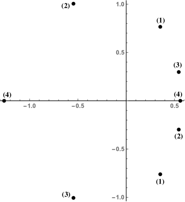
Figure 1: Equilibria of system (7). Each equilibrium is represented by the two points $\hat{z}^{(j)}_{1}$ and $\hat{z}^{(j)}_{2}$ labeled by the index $j=1,2,3,4$, see (12).

Below we provide graphs of the real and imaginary parts of the components of the solution $(z_{1}\left(t\right),z_{2}(t))$ of system (7) as functions of time, and some trajectories of the particles $z_{1}$ and $z_{2}$ in the complex $z$-plane. These graphs have been obtained by solving system (7) numerically using Mathematica.

(7a) Initial conditions $z_{1}(0)=\hat{z}^{(1)}_{1}+0.01$, $z_{2}(0)=\hat{z}^{(1)}_{2}+0.01$,

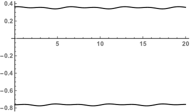
Figure 2: System (7), initial conditions (7a). Graphs of the real and imaginary parts of the coordinate $z_{1}(t)$.

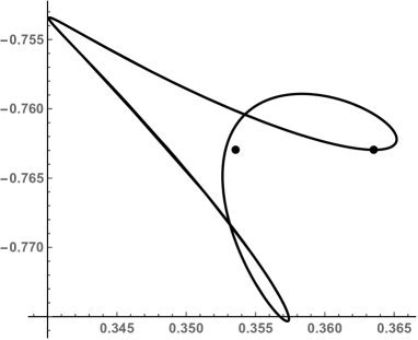
Figure 3: System (7), initial conditions (7a). Trajectory, in the complex $z$-plane, of $z_{1}(t)$. The two dots on the figure indicate the positions of $\hat{z}^{(1)}_{1}$ respectively ${z}_{1}(0)$, i.e. of a nearby equilibrium point respectively the initial value of $z_{1}(t)$.

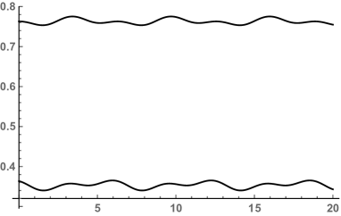
Figure 4: System (7), initial conditions (7a). Graphs of the real and the imaginary parts of the coordinate $z_{2}(t)$.

$\dot{z}_{1}(0)=0.01$, $\dot{z}_{2}(0)=-0.01$. See Figures 2, 3, 4, 5.

(7b) Initial conditions $z_{1}(0)=\hat{z}^{(1)}_{1}+0.01+0.01~{}\mathbf{i}$, $z_{2}(0)=\hat{z}^{(1)}_{2}+0.01+0.01~{}\textbf{i}$,

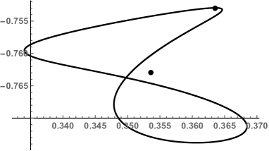
Figure 6: System (7), initial conditions (7b). Trajectory, in the complex $z$-plane, of $z_{1}(t)$. The two dots on the figure indicate the positions of $\hat{z}^{(1)}_{1}$ respectively ${z}_{1}(0)$, i.e. of a nearby equilibrium point respectively the initial value of $z_{1}(t)$.

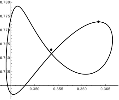
Figure 7: System (7), initial conditions (7b). Trajectory, in the complex $z$-plane, of $z_{2}(t)$. The two dots on the figure indicate the positions of $\hat{z}^{(1)}_{2}$ respectively ${z}_{2}(0)$, i.e. of a nearby equilibrium point respectively the initial value of $z_{2}(t)$.

$\dot{z}_{1}(0)=-0.01$, $\dot{z}_{2}(0)=0.01$. See Figures 6, 7.

(7c) Initial conditions $z_{1}(0)=\hat{z}^{(2)}_{1}+0.01+0.01~{}\mathbf{i}$, $z_{2}(0)=\hat{z}^{(2)}_{2}+0.01+0.01~{}\mathbf{i}$,

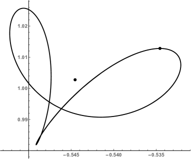
Figure 8: System (7), initial conditions (7c). Trajectory, in the complex $z$-plane, of $z_{1}(t)$. The two dots on the figure indicate the positions of $\hat{z}^{(2)}_{1}$ respectively ${z}_{1}(0)$, i.e. of a nearby equilibrium point respectively the initial value of $z_{1}(t)$.

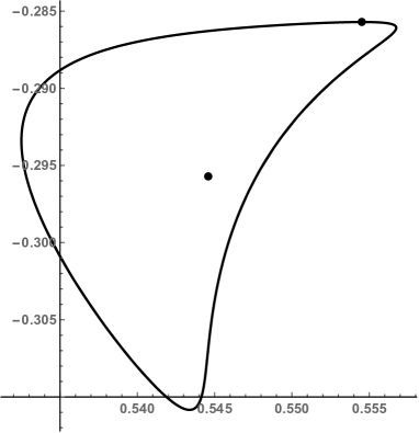
Figure 9: System (7), initial conditions (7c). Trajectory, in the complex $z$-plane, of $z_{2}(t)$. The two dots on the figure indicate the positions of $\hat{z}^{(2)}_{2}$ respectively ${z}_{2}(0)$, i.e. of a nearby equilibrium point respectively the initial value of $z_{2}(t)$.

$\dot{z}_{1}(0)=-0.01$, $\dot{z}_{2}(0)=0.01$. See Figures 8, 9.

(7d) Initial conditions $z_{1}(0)=\hat{z}^{(3)}_{1}+0.01+0.01~{}\mathbf{i}$, $z_{2}(0)=\hat{z}^{(3)}_{2}+0.01+0.01~{}\mathbf{i}$,

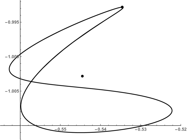
Figure 10: System (7), initial conditions (7d). Trajectory, in the complex $z$-plane, of $z_{1}(t)$. The two dots on the figure indicate the positions of $\hat{z}^{(3)}_{1}$ and ${z}_{1}(0)$, i.e. of a nearby equilibrium point respectively the initial value of $z_{1}(t)$.

$\dot{z}_{1}(0)=-0.005$, $\dot{z}_{2}(0)=0.005$. See Figures 10 and 11.

(7e) Initial conditions $z_{1}(0)=\hat{z}^{(4)}_{1}+0.01+0.01~{}\mathbf{i}$, $z_{2}(0)=\hat{z}^{(4)}_{2}+0.01+0.01~{}\mathbf{i}$,

$\dot{z}_{1}(0)=-0.01$, $\dot{z}_{2}(0)=0.01$. See Figures 10 and 11.

Example 2.2. For $N=3$ and $\omega=1$, taking into account that $c_{1}=-z_{1}-z_{2}-z_{3}$, $c_{2}=z_{1}z_{2}+z_{1}z_{3}+z_{2}z_{3}$, and $c_{3}=-z_{1}z_{2}z_{3}$, we see that system (2) reduces to

$$\ddot{z}_{1}=\frac{2\dot{z}_{1}\dot{z}_{2}}{z_{1}-z_{2}}+\frac{2\dot{z}_{1}\dot{z}_{3}}{z_{1}-z_{3}}$$

$$-\frac{1}{(z_{1}-z_{2})(z_{1}-z_{3})}\left[z_{1}^{2}F_{1}(z_{1},z_{2},z_{3})+z_{1}F_{2}(z_{1},z_{2},z_{3})+F_{3}(z_{1},z_{2},z_{3}))\right],$$

$$\ddot{z}_{2}=-\frac{2\dot{z}_{1}\dot{z}_{2}}{z_{1}-z_{2}}+\frac{2\dot{z}_{2}\dot{z}_{3}}{z_{2}-z_{3}}$$

$$+\frac{1}{(z_{1}-z_{2})(z_{2}-z_{3})}\left[z_{2}^{2}F_{1}(z_{1},z_{2},z_{3})+z_{2}F_{2}(z_{1},z_{2},z_{3})+F_{3}(z_{1},z_{2},z_{3}))\right],$$

$$\ddot{z}_{3}=-\frac{2\dot{z}_{1}\dot{z}_{3}}{z_{1}-z_{3}}-\frac{2\dot{z}_{2}\dot{z}_{3}}{z_{2}-z_{3}}$$

$$-\frac{1}{(z_{1}-z_{3})(z_{2}-z_{3})}\left[z_{3}^{2}F_{1}(z_{1},z_{2},z_{3})+z_{3}F_{2}(z_{1},z_{2},z_{3})+F_{3}(z_{1},z_{2},z_{3}))\right],$$

(13a)

where

$$F_{1}(z_{1},z_{2},z_{3})=z_{1}+z_{2}+z_{3}-\frac{2}{(z_{1}+z_{2}+z_{3}-z_{1}z_{2}z_{3})^{3}}$$

$$-\frac{2}{(z_{1}+z_{2}+z_{3}+z_{1}z_{2}+z_{1}z_{3}+z_{2}z_{3})^{3}},$$

$$F_{2}(z_{1},z_{2},z_{3})=-z_{1}z_{2}-z_{1}z_{3}-z_{2}z_{3}$$

$$+\frac{2}{(z_{1}+z_{2}+z_{3}+z_{1}z_{2}+z_{1}z_{3}+z_{2}z_{3})^{3}}+\frac{2}{(z_{1}z_{2}+z_{1}z_{3}+z_{2}z_{3}+z_{1}z_{2}z_{3})^{3}},$$

$$F_{3}(z_{1},z_{2},z_{3})=z_{1}z_{2}z_{3}$$

$$+\frac{2}{(z_{1}+z_{2}+z_{3}-z_{1}z_{2}z_{3})^{3}}-\frac{2}{(z_{1}z_{2}+z_{1}z_{3}+z_{2}z_{3}+z_{1}z_{2}z_{3})^{3}}.$$ (13b)

We obtained equilibria of system  (13) as follows. First, we found the equilibria of system (4) for $N=3$; they are given by $(0,\sqrt{\frac{3}{2}},-\sqrt{\frac{3}{2}})$ and $(0,\mathbf{i}\sqrt{\frac{3}{2}},-\mathbf{i}\sqrt{\frac{3}{2}})$, up to the permutations of the three coordinates. Second, we found the zeros of the monic polynomials whose coefficients are the equilibria of system (4) for $N=3$. These zeros are equilibriumum solutions of system (2) because of how this system is constructed. Therefore, system (13) has at least 12 equilibrium configurations $(\hat{z}^{(j)}_{1},\hat{z}^{(j)}_{2},\hat{z}^{(j)}_{3})$, $j=1,2,\ldots,12$, up to the permutations of $\hat{z}^{(j)}_{1}$, $\hat{z}^{(j)}_{2}$ and $\hat{z}^{(j)}_{3}$, whose approximate numerical values are given below:

$$\begin{array}[]{l}(\hat{z}^{(1)}_{1},\hat{z}^{(1)}_{2},\hat{z}^{(1)}_{3})=(0.720239-0.575751~{}\mathbf{i},0.720239+0.575751~{}\mathbf{i},-1.44048),\\ (\hat{z}^{(2)}_{1},\hat{z}^{(2)}_{2},\hat{z}^{(2)}_{3})=(0.397225+1.07661~{}\mathbf{i},-1.12106-0.854451~{}\mathbf{i},0.72384-0.222154~{}\mathbf{i}),\\ (\hat{z}^{(3)}_{1},\hat{z}^{(3)}_{2},\hat{z}^{(3)}_{3})=(0.397225-1.07661~{}\mathbf{i},0.72384+0.222154~{}\mathbf{i},-1.12106+0.854451~{}\mathbf{i}),\\ (\hat{z}^{(4)}_{1},\hat{z}^{(4)}_{2},\hat{z}^{(4)}_{3})=(0.709,-0.3545-1.2656~{}\mathbf{i},-0.3545+1.2656~{}\mathbf{i}),\\ (\hat{z}^{(5)}_{1},\hat{z}^{(5)}_{2},\hat{z}^{(5)}_{3})=(-0.781352,1.00305-0.749241~{}\mathbf{i},1.00305+0.749241~{}\mathbf{i}),\\ (\hat{z}^{(6)}_{1},\hat{z}^{(6)}_{2},\hat{z}^{(6)}_{3})=(0,0.612372-0.921816~{}\mathbf{i},0.612372+0.921816~{}\mathbf{i}),\\ (\hat{z}^{(7)}_{1},\hat{z}^{(7)}_{2},\hat{z}^{(7)}_{3})=(-0.82853-0.22063~{}\mathbf{i},0.82853-0.22063~{}\mathbf{i},1.666~{}\mathbf{i}),\\ (\hat{z}^{(8)}_{1},\hat{z}^{(8)}_{2},\hat{z}^{(8)}_{3})=(0,-0.673004+1.52228~{}\mathbf{i},0.673004-0.297537~{}\mathbf{i}),\\ (\hat{z}^{(9)}_{1},\hat{z}^{(9)}_{2},\hat{z}^{(9)}_{3})=(0.82853+0.22063~{}\mathbf{i},-1.666~{}\mathbf{i},-0.82853+0.22063~{}\mathbf{i}),\\ (\hat{z}^{(10)}_{1},\hat{z}^{(10)}_{2},\hat{z}^{(10)}_{3})=(0,-0.673004-1.52228~{}\mathbf{i},0.673004+0.297537~{}\mathbf{i}),\\ (\hat{z}^{(11)}_{1},\hat{z}^{(11)}_{2},\hat{z}^{(11)}_{3})=(-1.00305+0.749241~{}\mathbf{i},-1.00305-0.749241~{}\mathbf{i},0.781352),\\ (\hat{z}^{(12)}_{1},\hat{z}^{(12)}_{2},\hat{z}^{(12)}_{3})=(0,-1.87718,0.652438).\end{array}$$ (26)

It is possible that the system of algebraic equations characterizing the equilibria of (13) has additional solutions besides those listed above. A direct attempt to solve this system of algebraic equations using Mathematica was unsuccessful, and we did not deem the matter surficiently relevant to justify further investigations.

In Figure 14 each equilibrium of system (13) is represented by the three points $\hat{z}^{(j)}_{1}$, $\hat{z}^{(j)}_{2}$ and $\hat{z}^{(j)}_{3}$, where $j=1,2,\ldots,12$. We leave it to the interested reader to compare Figure 14 with the list of equilibria (26), in order to locate the triples that correspond to each of the 12 equilibria.

Below we provide some trajectories, in the complex plane, of the particles $z_{1}$, $z_{2}$ and $z_{3}$ whose evolution is described by system (13) with the initial conditions

$$z_{1}(0)=\hat{z}^{(3)}_{1}+0.1,\dot{z}_{1}(0)=0.1,$$

$$z_{2}(0)=\hat{z}^{(3)}_{2}+0.1,\dot{z}_{2}(0)=0.1,$$

$$z_{3}(0)=\hat{z}^{(3)}_{3}+0.1,\dot{z}_{3}(0)=0.1,$$ (27)

see Figures 15, 16 and 17. These graphs have been obtained by solving system (13) with the initial conditions (27) numerically using Mathematica.

Figure 5: System (7), initial conditions (7a). Trajectory, in the complex $z$-plane, of $z_{2}(t)$. The two dots on the figure indicate the positions of $\hat{z}^{(1)}_{2}$ respectively ${z}_{2}(0)$, i.e of a nearby equilibrium point respectively the initial value of $z_{2}(t)$.

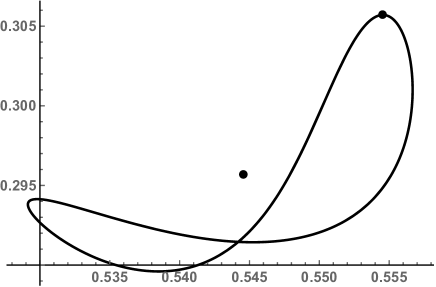
Figure 11: System (7), initial conditions (7d). Trajectory, in the complex $z$-plane, of $z_{2}(t)$. The two dots on the figure indicate the positions of $\hat{z}^{(3)}_{2}$ and ${z}_{2}(0)$, i.e. of a nearby equilibrium point respecttively the initial value of $z_{2}(t)$.

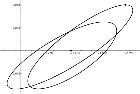
Figure 12: System (7), initial conditions (7e). Trajectory, in the complex $z$-plane, of $z_{1}(t)$. The two dots on the figure indicate the positions of $\hat{z}^{(4)}_{1}$ and ${z}_{1}(0)$, i.e. of a nearby equilibrium point respectively the initial value of $z_{1}(t)$.

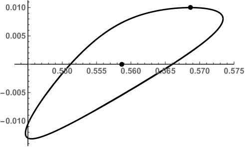
Figure 13: System (7), initial conditions (7e). Trajectory, in the complex $z$-plane, of $z_{2}(t)$. The two dots on the figure indicate the positions of $\hat{z}^{(4)}_{2}$ and ${z}_{2}(0)$, i.e. of a nearby equilibrium point respectively the initial value of $z_{2}(t)$.

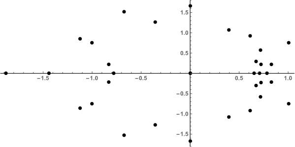
Figure 14: Equilibria of system (13). Each equilibrium is represented by the three points $\hat{z}^{(j)}_{1}$, $\hat{z}^{(j)}_{2}$ and $\hat{z}^{(j)}_{3}$ indexed by $j=1,2,\ldots,12$, see (26).

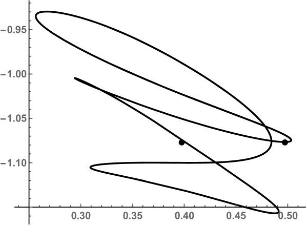
Figure 15: System (13), initial conditions (27). Trajectory, in the complex $z$-plane, of $z_{1}(t)$. The two dots on the figure indicate the positions of $\hat{z}^{(3)}_{1}$ respectively ${z}_{1}(0)$, i.e. of a nearby equilibrium point respectively the initial value of $z_{1}(t)$.

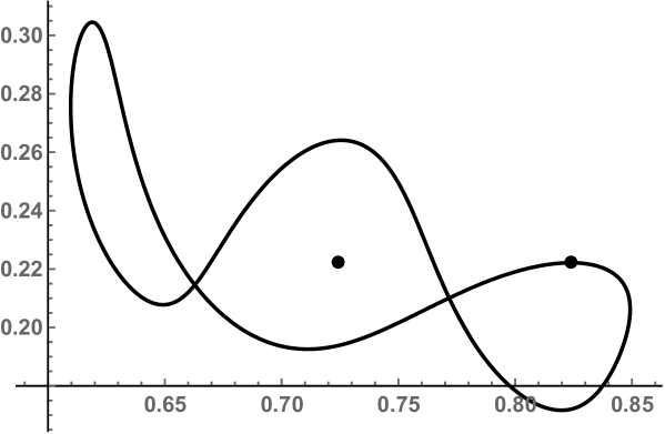
Figure 16: System (13), initial conditions (27). Trajectory, in the complex $z$-plane, of $z_{2}(t)$. The two dots on the figure indicate the positions of $\hat{z}^{(3)}_{2}$ and ${z}_{2}(0)$, i.e. of a nearby equilibrium point respectively the initial value of $z_{2}(t)$.

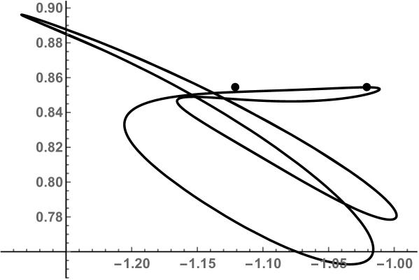
Figure 17: System (13), initial conditions (27). Trajectory, in the complex $z$-plane, of $z_{3}(t)$. The two dots on the figure indicate the positions of $\hat{z}^{(3)}_{3}$ and ${z}_{3}(0)$, i.e. of a nearby equilibrium point respectively the initial value of $z_{3}(t)$.

3 Outlook

The interest of the many-body model introduced and discussed above is demonstrated by its solvable and isochronous character as well as by the remarkable trajectories it features – already in the simple $N=2$ and $N=3$ cases, as shown by the graphs reported above. It is also amusing to observe—as the cognoscienti will have noted—that this solvable model has been obtained by appropriately combining the two solvable equations—see (1a) and (4)—which are the prototypes of two, quite different, basic families of solvable many-body problems of Newtonian type. Moreover—as reported in [7]—the findings reported above provide the point of departure to obtain Diophantine properties of the $N$ zeros of each of the $N!$ (monic) polynomials the coefficients of which are the $N$ zeros of the Hermite polynomial $H_{N}\left(z\right)$ of degree $N$ (these $N!$ polynomials correspond of course to the $N!$ permutations of the $N$ zeros of $H_{N}\left(z\right)$). And a rather ample vista of further developments is provided by these findings.

References

- [1] F. Calogero, “The “neatest” many-body problem amenable to exact treatments (a “goldfish”?)”, Physica D 152-153, 78-84 (2001).
- [2] F. Calogero, “Motion of Poles and Zeros of Special Solutions of Nonlinear and Linear Partial Differential Equations, and Related “Solvable” Many Body Problems”, Nuovo Cimento 43B, 177-241 (1978).
- [3] F. Calogero, Classical many-body problems amenable to exact treatments, Lecture Notes in Physics Monographs m66, Springer, Heidelberg, 2001.
- [4] F. Calogero, Isochronous systems, Oxford University Press, Oxford, 2008; marginally updated paperback edition 2012.
- [5] D. Gómez-Ullate and M. Sommacal, “Periods of the Goldfish Many-Body Problem”, J. Nonlinear Math. Phys. 12, Suppl. 1, 351–362 (2005).
- [6] F. Calogero, “New solvable variants of the goldfish many-body problem”, Studies Appl. Math. (submitted to, 20.05.2015).
- [7] O. Bihun and F. Calogero, “Diophantine properties of the zeros of (monic) polynomials the coefficients of which are the zeros of Hermite polynomials”, SIGMA (submitted to).
- [8] A. Erdélyi (editor), Higher transcendental functions, vol. II, McGraw-Hill, New York, 1953.
- [9] M. A. Olshanetsky and A. M. Perelomov, “Classical integrable finite-dimensional systems related to Lie algebras”, Phys. Rep. 71, 313–400 (1981).