Spectral Detection on Sparse Hypergraphs

Abstract

We consider the problem of the assignment of nodes into communities from a set of hyperedges, where every hyperedge is a noisy observation of the community assignment of the adjacent nodes. We focus in particular on the sparse regime where the number of edges is of the same order as the number of vertices. We propose a spectral method based on a generalization of the non-backtracking Hashimoto matrix into hypergraphs. We analyze its performance on a planted generative model and compare it with other spectral methods and with Bayesian belief propagation (which was conjectured to be asymptotically optimal for this model). We conclude that the proposed spectral method detects communities whenever belief propagation does, while having the important advantages to be simpler, entirely nonparametric, and to be able to learn the rule according to which the hyperedges were generated without prior information.

I Introduction

Detecting information about the vertex properties that is hidden (or encoded) in the structure of a graph is a central issue in many problems in physics, biology and computer science. In fact, many systems of interest are composed of a large number of variables about which we do not have any information but the relationships (or part of the relationships) between them. Starting from this knowledge we aim at inferring individual properties of the nodes.

In this context, the main approaches are statistical inference, where the detection is based on the assumption of a generative model for the graph [1, 2], and spectral methods [3]. For some classes of generative models, statistical inference methods based on belief propagation were predicted to be optimal in detecting planted hidden configurations [4, 5, 6]. Spectral methods have the great advantage of being non-parametric, meaning that they do not require any knowledge of the generative model (if one exists) and are completely independent of it. Nonetheless, standard spectral methods such as the adjacency matrix or the Laplacian succeed down to the information theoretical limit when the graph is sufficiently dense or regular [7, 8, 9, 10, 11] while tend to fail when graphs are sparse due to their sensitivity to fluctuations in the vertex degree.

These problems have been well studied in the case of graphs with simple edges between couples of vertices. However, many networks have a different structure, and the relationships between vertex-variables are not established in couples but in $k$-uplets, with $k>2$. An exemple is given, for instance, by the network of scientific collaborations, of skype conference calls, email exchanges or recommendation systems where we can associate a user with a specific content and a rating. Translating the hypergraph into pairwise interaction would inevitably lead to a loss of information, and therefore some effort has been made to generalize spectral methods to multi-body interactions [12, 13, 14].

Here we study an extension of the spectral clustering method proposed in [15] based on a generalization of the non-backtracking matrix [16, 15] to the case of hypergraphs (or factor graphs), that we argue to be effective on sparse networks. To test the performance of the spectral method we study it on a generative stochastic block model of hypergraphs similar to the ones defined in [17, 12] which is relevant for different problems ranging from community detection to planted constraint satisfiability. We compare the results with statistical inference based on belief propagation, which we also derive, and show the intimate connections between the latter and the non-backtracking operator. We also illustrate that on the sparse networks we consider, other spectral methods based on standard operators fail in the detection where the method we propose succeeds.

A particularly remarkable point about the method is that it works without any prior knowledge of the generative model or its parameters, it is hence a promising tool to learn the probabilistic rules that were used to create the hypergraph. We illustrate this on the example of planted constraint satisfaction problems where information about the nature of the constraints is not assumed but inferred.

The paper is organized as follows: In Sec. II we give the form of the generalized non-backtracking matrix and summarize the algorithm. In Sec. III we present the generative model. In Sec. IV we then discuss the performance of the algorithm on hypergraphs generated by the model. In Sec. V we derive the belief propagation algorithm and the detectability phase transition by linearization around the uniform fixed point. In Sec. VI-A and VI-B we apply the spectral algorithm to two specific cases of the generative model, namely an assortative stochastic block model and the planted $2$-in-$4$-sat, comparing its behavior and phase transitions with the one of belief-propagation. Finally in Sec. VII we give our conclusions.

II Spectral Detection Algorithm

Consider a hypergraph $G(V,E)$, with vertices $V$ with $|V|=N$, and hyperedges $E$, $|E|=M$. We denote by $\partial\mu$ the set of vertices included in the hyperedge $\mu$. Each vertex $i$ has an associated variable $a_{i}$ that can take values in the set ${\cal A}=\{0,\cdots,q-1\}$. These variables are hidden from us, but it is assumed that the hyperedges were chosen in a way that depends on the values of these variables. The goal is to infer the variables from the structure of the hypergraph.

The spectral algorithm we propose to detect hidden labels of the vertices in a sparse hypergraph is based on the following hypergraph non-backtracking operator

$$B_{(i\rightarrow\mu)(j\rightarrow\nu)}=\begin{cases}1&\text{if }j\in\partial\mu\backslash i\,\,,\,\,\nu\neq\mu\,,\\ 0&\text{otherwise}\,,\end{cases}$$ (1)

where $i,j=1,\cdots,N$ are vertex indices and $\mu,\nu=1,\cdots,M$ are hyper-edges (or factors). In Fig. 1 we show a graphical representation of one non-null element of the matrix. Vertices are represented by circles and hyperedges by squares. Each hyper-edge can be seen as a group of $k_{\mu}$ edges going from the participating vertices to the factor $\mu$. The matrix is therefore of size $\overline{k}M\times\overline{k}M$, where $M$ is the number of factors and

$$\overline{k}=\frac{1}{M}\sum_{\mu}\,k_{\mu}$$ (2)

is the average degree of a factor.

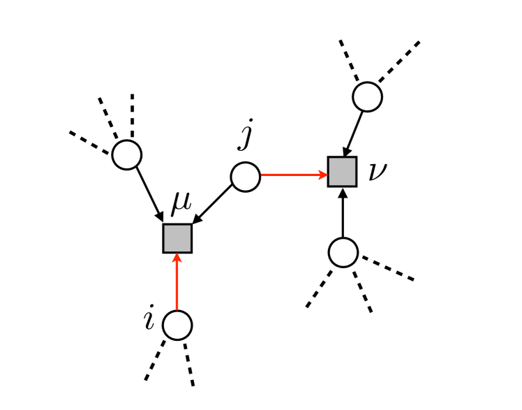
Figure 1: A graphical representation of one non-zero element $B_{(i\rightarrow\mu)(j\rightarrow\nu)}$ of the generalized non-backtracking matrix, where grey squares represent hyper-edges (or factors) and white circles are vertices.

This matrix has multiple advantages with respect to the use of adjacency or incidence matrix, in particular the fact that it is non-backtracking inhibits the eigenvalues linked to high degree vertices and the bulk of the spectrum is confined in a circle in the complex plane for large random networks.

The algorithm is the following:

• Given the hypergraph, construct the non-backtracking matrix according to (1).

• Compute the largest norm eigenvalues (and associated eigenvectors) down to the first that has a non-zero imaginary part. In this way we obtain $q$ eigenvalue-eigenvector pairs. Given that the first eigenvector is associated to the degree of the vertices, we retain the subsequent $q-1$ to identify a partition in $q$ groups.

• For each of the $q$ eigenvectors ${\bf v}$ construct an $N$ component vector ${\bf u}$ as

  $$u_{i}=\sum_{\mu\in\partial i}v_{i\rightarrow\mu}\,,$$ (3)

  where $\partial i$ indicates the set of factors to which vertex $i$ participates.

• Run the preferred clustering algorithm, for example soft $k$-means, on the components of the $q-1$ eigenvectors ${\bf u}$ to obtain a partition of the vertices in $q$ groups.

The algorithm we propose can be applied to any kind of hypergraphs with any distribution of vertex and factor degrees.

The other spectral method we consider for comparison is based on the adjacency matrix $A$, whose elements $a_{ij}$ are the number of hyper-edges containing both the vertices $i$ and $j$. The adjacency matrix of a hypergraph can be written in terms of the incidence matrix $H$ as $A=HH^{T}-D$, where the incidence matrix is an $N\times M$ matrix such that

$$H_{i\mu}=\begin{cases}1\quad\quad i\in\partial\mu\,,\\ 0\quad\quad{\rm otherwise}.\end{cases}$$ (4)

In the following we specify a generative model on which we will analyze the performance of our non-backtracking algorithm comparing it with the ground truth and other algorithms.

III The Model

Consider a set of vertices $V$ with $|V|=N$, where each vertex variable $a_{i}$ can take values in the set ${\cal A}=\{0,\cdots,q-1\}$. Each vertex is independently assigned a value $a\in{\cal A}$ with a probability $n_{a}$ such that $\sum_{a}n_{a}=1$.

Consider now a kernel function ${\mathcal{P}}:{\cal A}^{k}\rightarrow{\rm I\!R}_{[0,1]}$ that is symmetric under any permutation of the arguments and represented by the symmetric $k$-tensor ${\bf p}$ (although generalization to non-symmetric kernels should not present any particular difficulty). Let ${\cal E}^{(k)}$ be the set of all the possible hyper-edges of degree $k$ between the $N$ vertices, the kernel tensor gives the probability of existence, independently, for any hyper-edge in ${\cal E}^{(k)}$. To every hyper-edge in ${\cal E}^{(k)}$ is associated an indicator variable $e_{\mu}$ with $\mu=1,\cdots,\binom{N}{k}$, with probability

$${\rm Prob}\left(e_{\mu}=1|\,\underline{a}_{\mu}\right)=p_{\underline{a}_{\mu}}\,,$$ (5)

where $\underline{a}_{\mu}\in{\cal A}^{k}$ is the set of labels planted on the vertices participating to the hyper-edge $\mu$. The hypergraph is fully specified by the vector ${\bf e}$. The expected number of edges in the hypergraph is given by

$$M=\mathbb{E}\left[\sum_{\mu}e_{\mu}\right]\,.$$ (6)

We are interested in the sparse case, i.e. $M=O(N)$, therefore the elements of the tensor must scale as

$$p_{\underline{a}}=\frac{c_{\underline{a}}}{N^{k-1}}\,,$$ (7)

where $c_{\underline{a}}=O(1)$. In the following, with a slight abuse of notation, $\underline{a}$ will indicate a variable in ${\cal A}^{k}$, ${\cal A}^{k-1}$ or ${\cal A}^{k-2}$, which one of the three will be clear in the context.

In the large $N$ limit at leading order the expected degree of a node with a label $a$ is

$$c_{a}=\frac{1}{(k-1)!}\sum_{\underline{b}\in{\cal A}^{k-1}}c_{a,\underline{b}}\prod_{l=1}^{k-1}n_{b_{l}}\,.$$ (8)

It will also be useful in the following to define the two-vertices average degree, namely

$$c_{ab}=\frac{1}{(k-2)!}\sum_{\underline{s}\in{\cal A}^{k-2}}c_{ab,\underline{s}}\prod_{l=1}^{k-2}n_{s_{l}}\,.$$ (9)

Given the planted assignment $\{a_{i}\}$, the conditional probability of generating a certain hypergraph $G$ specified by the set of indicator variables $\{e_{\mu}\}$ is

$$P(G|\{a_{i}\}_{i=1,\dots,N})=\prod_{\mu\in{\cal E}^{(k)}}\left[\left(\frac{c_{\underline{a}_{\mu}}}{N^{k-1}}\right)^{e_{\mu}}\left(1-\frac{c_{\underline{a}_{\mu}}}{N^{k-1}}\right)^{1-e_{\mu}}\right]\,.$$ (10)

As anticipated in the introduction, this generative model covers a wide range of problems of which we give some examples below.

• Planted Constraint Satisfaction Problems. Constraint satisfaction problems play a crucial role in theoretical and applied computer science as well as in engineering and physics due to their very general nature. In a CSP we consider a set of $N$ discrete variables, typically Boolean, subject to a set of $M$ constraints. In many of the usually considered cases like $k$-SAT or $k$-XORSAT or $k$-in-$2k$-SAT these constraints are all of the same type. In $k$-SAT, for example, the OR between $M$ $k$-uples of variables (or their negations) must result to TRUE. In a random CSP the constraints are thrown at random between groups of variables, giving raise to a random graph. The question is if we can find a satisfying assignment. In a planted CSP [18, 19, 20, 21] we throw at random an assignment of the variables and then a series of constraints (factors or hyper-edges) that are satisfied by the assignment itself. The question is if and how, given the graph, we can recover the planted assignment. Planted CSPs are covered by the above generative model.

• Hypergraph Stochastic Block Models. The stochastic block model is a popular way of generating graphs with a community structure. An ensemble of $N$ vertices is labeled with values from $1$ to $q$ depending on which of the $q$ communities they belong to. Given this assignment, edges between couples of nodes are thrown at random with a probability (kernel) that depends on the labeling of the two nodes that participate to the edge. Two typical choices are the assortative case where nodes belonging to the same community are more likely to be connected or disassortative if the case is the opposite. Again, the objective is, given the graph, recover the underlying community structure. Our model is the natural generalization of the stochastic block model to the case of hypergraphs, which is relevant in many applications, from recommendation systems to co-authoring networks.

• Coding. If we allow, in the planted CSP scenario, the constraints to be soft, meaning that they can be violated with a certain finite probability, the hypergraph can be seen as a noisy observation of the data, where the data consist in the planted assignment. In many cases encoding is performed by summing a random set of variables and transmitting the sum through a noisy channel. The choice of the sets results in a random hyper-graph with a structure that is determined by the code construction and the transmission gives a noisy version of this hypergraph. Our generative model can also be seen as a representation of this kind of setting.

For the analysis of this paper we will consider the case where the average degree of the vertices is independent of the labeling, namely $c_{a}=c$. This is the statistically hardest case, because simply observing the degree of a node does not give any information about its planted variable. In doing so we obtain a random sparse hypergraph with structure but in which degrees of all the vertices come from Poisson distribution with average $c$.

The performance of a detection algorithm can be evaluated through a measure of the normalized overlap between the planted assignment and the inferred one, namely

$$Q=\max_{\pi}\frac{\frac{1}{N}\sum_{i}\delta_{a_{i},\pi(\hat{a}_{i})}-\max_{a}n_{a}}{1-\max_{a}n_{a}}$$ (11)

where ${\bf a}$ is the planted assignment, $\hat{{\bf a}}$ is the inferred assignment and $\pi$ is any permutation of the labels.

IV Properties of $B$ on the planted model

In this section we present the properties of the non-backtracking matrix for a hypergraph generated with the above planted model.

First we remark that the hypergraph can be seen as a bipartite graph between the variable nodes and the hyperedges. In the case this bipartite graph is random (non-planted, but fixed degree sequence), results derived for the spectrum of the non-backtracking operator of this bipartite graph in [15, 22] translate directly to the present case.

The largest eigenvalue of $B$ is, asymptotically in the large $N$ limit, equal to the average branching factor of the locally tree-like hypergraph. For a $k$-regular hypergraph this reads

$$\mu_{1}=(k-1)\mathbb{E}_{Q}\left[d\right]\,,$$ (12)

where $Q_{d}=(d+1)p_{d+1}/c$ is the excess degree distribution and $p_{d}$ is the degree distribution. Since we are considering Poissonian degree, for the first eigenvalue we find

$$\mu_{1}=c(k-1)\,.$$ (13)

The bulk of the spectrum is confined in the circle of radius

$$\rho=\sqrt{c(k-1)}\,.$$ (14)

This can be seen by considering that for any matrix $B$ with eigenvalue $\mu$

$$\sum_{i=1}^{kM}|\mu|^{2r}<\text{Tr}(B^{r})(B^{r})^{T}\,.$$ (15)

Moreover, for any fixed $r$ and in the limit $N\rightarrow\infty$, the hypergraph is locally tree-like, therefore the diagonal elements $(i\rightarrow\mu)(i\rightarrow\mu)$ of $(B^{r})(B^{r})^{T}$ count the exact number of factor nodes at $r$ steps from $\mu$ through paths not including $i$, which in expectation is $(k-1)^{r}c^{r}$. Therefore for the trace we obtain

$$\mathbb{E}\left[\text{Tr}(B^{r})(B^{r})^{T}\right]=kM(k-1)^{r}c^{r}\,,$$ (16)

which gives

$$\mathbb{E}\left[|\mu|^{2r}\right]\leq(k-1)^{r}c^{r}\,.$$ (17)

Since this relation is true for any fixed value of $r$, we conclude that almost all the eigenvalues of the non-backtracking matrix lie in the circle of radius (14). More refined analysis of [22] leads to the result that for a random hypergraph all but one eigenvalue lie in that circle.

The planted model can be seen as a perturbed rank-$r$ matrix. If the rescaled eigenvalues of the non-perturbed rank $r$ matrix fall outside of the circle confining the bulk then they are also visible on the real axes in the spectrum of the non-backtracking operator. Hence, in analogy with [15, 22] the second $q-1$ eigenvalues, when exceeding the bulk, are associated to eigenvectors that are correlated with the planted configuration and take values

$$\mu_{2}=c(k-1)\lambda\,,$$ (18)

where $\lambda$ is one of the largest $q-1$ eigenvalues of the matrix

$$T_{ab}=n_{a}\left[\frac{c_{ab}}{c(k-1)}-1\right]\,,$$ (19)

which, as we will see, are degenerate under appropriate conditions.

Inference of the planted assignment can be performed through a standard clustering algorithm like $k$-means applied to these eigenvectors when the informative eigenvalues exceed the bulk, namely

$$|\mu_{2}|>\sqrt{c(k-1)}\,.$$ (20)

The vectors that we cluster are constructed from the eigenvectors of $B$ by summing all the outgoing edges for each vertex.

The algorithm hence requires to find the leading eigenvalues of a $\overline{k}M\times\overline{k}M$ matrix, which can be very large if the average degree of the nodes is high. Nonetheless, if the hypergraph is $k$-regular as we are considering, we can reduce the size of the problem. The eigenvalue equation we are solving is the following

$$\sum_{\nu\in\partial i\backslash\mu}\sum_{k\in\partial\nu\backslash i}v_{k\rightarrow\nu}=\mu v_{i\rightarrow\mu}\,.$$ (21)

Let us consider the sums of incoming and outgoing messages, respectively

$$\begin{split}v^{\rm in}_{i}&=\sum_{\nu\in\partial i}\sum_{k\in\partial\nu\backslash i}v_{k\rightarrow\nu}\,,\\ v^{\rm out}_{i}&=\sum_{\nu\in\partial i}v_{i\rightarrow\nu}\,,\end{split}$$ (22)

for which the eigenvalue equation (21) translates into

$$\begin{split}(d_{i}-1)v^{\rm in}_{i}&=\lambda v^{\rm out}_{i}\,,\\ \sum_{\mu\in\partial i}\sum_{j\in\partial\mu\backslash i}v^{\rm in}_{j}-(k-2)v^{\rm in}_{i}-(k-1)v^{\rm out}_{i}&=\lambda v^{\rm in}_{i}\,.\end{split}$$ (23)

The preceding equation can be written in a compact form as

$$B^{\prime}{\bf v}=\lambda{\bf v}\,,$$ (24)

with

$${\bf v}=\left(\begin{matrix}{\bf v}^{\rm out}\\ {\bf v}^{\rm in}\end{matrix}\right)\,,$$ (25)

and

$$B^{\prime}=\left(\begin{matrix}0&D-\mathbb{1}\\ -(k-1)\mathbb{1}&A-(k-2)\mathbb{1}\end{matrix}\right)\,,$$ (26)

where $B^{\prime}$ is a $2N\times 2N$ matrix, $D$ is the diagonal degree matrix $A$ is the symmetric adjacency matrix. Given this, we see that all the eigenvalues of the complete non-backtracking operator $B$ are also eigenvalues of the reduced one $B^{\prime}$ except for those $kM-2N$ associated to the subspace defined by

$$\begin{split}\sum_{\nu\in\partial i}\sum_{k\in\partial\nu\backslash i}v_{k\rightarrow\nu}=0\quad\forall i\,,\\ \sum_{\nu\in\partial i}v_{i\rightarrow\nu}=0\quad\quad\forall i\,,\end{split}$$ (27)

for which we cannot assure the correspondence. Moreover, by a further transformation of the eigenvalue eq. (21), we can obtain the following non-linear equation describing the eigenvalues of the reduced operator

$$v_{i}=\frac{1}{1-\frac{\lambda(p-2+\lambda)}{p-1}}\left[d_{i}v_{i}-\frac{\lambda}{p-1}\sum_{\mu\in\partial i}\sum_{k\in\partial\mu\backslash i}v_{k}\right]$$ (28)

telling us that the differences between the $B$ and $B^{\prime}$ spectra will be located in $\lambda=1$ and $\lambda=-(p-1)$ due to the singularities that appear in the formula.

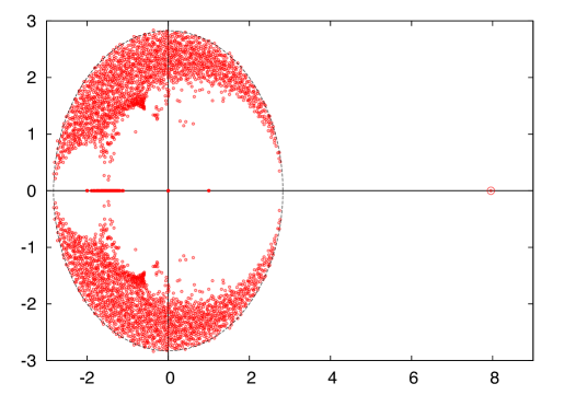
(a) (b) (c)

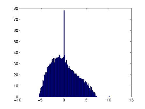
Figure 2: The spectrum of the hypergraph non-backtracking matrix (1) for an hypergraph of size $N=1800$ generated through the assortative HSBM with $k=3$, $q=3$ and $c=4$ for (a) $\tilde{\varepsilon}=0.22$ and (b) $\tilde{\varepsilon}=0.14$. In (b) the informative eigenvalues lie outside the bulk and are degenerate. (c) The spectrum of the adjacency matrix for $\tilde{\varepsilon}=0.14$. Despite being in the detectable phase the informative eigenvalue of the adjacency matrix is hidden in the bulk.

V Belief Propagation and Phase Transitions

In this section we derive the asymptotic properties of the generative model through belief propagation and, as a byproduct, we highlight the connection between belief propagation and the generalized non-backtracking operator.

Given the conditional probability of a graph (10), according to the Bayes rule the posterior probability of the planted assignment ${a_{i}}$ given the hypergraph $G$ reads

$$\begin{split}P(\{a_{i}\}_{i=1,\dots,N}|G)&=\frac{1}{Z(G)}\prod_{i=1}^{N}n_{a_{i}}\times\\ &\times\prod_{\mu\in{\cal E}^{(k)}}\left[c_{\underline{a}_{\mu}}^{e_{\mu}}\left(1-\frac{c_{\underline{a}_{\mu}}}{N^{k-1}}\right)^{1-e_{\mu}}\right]\,,\end{split}$$ (29)

where $Z(G)$ is the proper normalization constant. This posterior probability is associated to a graphical model for which we can write $2k|{\cal E}^{(k)}|$ coupled message-passing equations [23]

$$\begin{split}\psi_{a}^{\mu\rightarrow i}&=\frac{1}{Z^{\mu\rightarrow i}}\sum_{\underline{b}}\left(\prod_{j\in\partial\mu\backslash i}\chi^{j\rightarrow\mu}_{b_{j}}\right)\times\,,\\ &\times\left[c_{a,\underline{b}}^{e_{\mu}}\left(1-\frac{c_{a,\underline{b}}}{N^{k-1}}\right)^{1-e_{\mu}}\right]\,,\\ \chi^{i\rightarrow\mu}_{a}&=\frac{1}{\Theta^{i\rightarrow\mu}}\,n_{a}\,\prod_{\nu\in{\tilde{\partial}}i\backslash\mu}\psi_{a}^{\nu\rightarrow i}\,,\end{split}$$ (30)

where ${\tilde{\partial}}i$ indicates all the hyperedges in ${\cal E}^{(k)}$ that contain vertex $i$, $Z^{\mu\rightarrow i}$ and $\Theta^{i\rightarrow\mu}$ are normalization constants. The estimated marginal probability that a vertex was planted in the group $a$ is given by the associated belief, namely

$$\chi^{i}_{a}=\frac{1}{\Theta^{i}}\,n_{a}\,\prod_{\nu\in{\tilde{\partial}}i}\psi_{a}^{\nu\rightarrow i}\,.$$ (31)

By plugging the first equation of (30) into the second, we obtain a closed set of $k|{\cal E}^{(k)}|$ equations for the $\chi$ messages:

$$\begin{split}\chi^{i\rightarrow\mu}_{a}&=\frac{1}{K^{i\rightarrow\mu}}\,n_{a}\,\prod_{\nu\in{\tilde{\partial}}i\backslash\mu}\sum_{\underline{b}}\left(\prod_{j\in\partial\nu\backslash i}\chi^{j\rightarrow\nu}_{b_{j}}\right)\times\\ &\times\left[c_{a,\underline{b}}^{e_{\nu}}\left(1-\frac{c_{a,\underline{b}}}{N^{k-1}}\right)^{1-e_{\nu}}\right]\,.\end{split}$$ (32)

In order to reduce the number of equations we note that there are two different types of messages $i\rightarrow\mu$, namely the ones living on the $kM$ edges that actually exist in $G$, for which $i\in\partial\mu$ and $e_{\mu}=1$, and the “ghost” edges for which $i\notin\partial\mu$ and $e_{\mu}=0$.

It can be shown that, up to corrections that vanish when $N\rightarrow\infty$, for the “ghost” hyper-edges we have $\chi^{i\rightarrow\mu}_{a}\simeq\chi^{i}_{a}$, while for the messages living on the real edges

$$\chi^{i\rightarrow\mu}_{a}=\frac{e^{-h_{a}}}{K^{i\rightarrow\mu}}\,n_{a}\prod_{\nu\in\partial i\backslash\mu}\sum_{\underline{b}}\left(\prod_{j\in\partial\nu\backslash i}\chi^{j\rightarrow\nu}_{b_{j}}\right)\,c_{a,\underline{b}}\,,$$ (33)

with

$$h_{a}=\frac{1}{N^{k-1}}\sum_{\gamma\in{\cal E}^{(k-1)}}\sum_{\underline{b}}\,c_{a,\underline{b}}\,\left(\prod_{j\in\partial\gamma}\,\chi^{j}_{b_{j}}\right)\,,$$ (34)

which reduces the number of messages to $kM$. Still, the computation of the effective field $h_{a}$ requires the summation of order $N^{k-1}$ terms which for large hypergraphs becomes problematic as soon as $k>2$. We will show in Sec. VI that the computation of the field can be largely simplified when a specific choice of the connectivity tensor ${\bf c}$ is made.

It can be easily verified that, if the condition $c_{a}=c\,\,\forall a$ holds, then the so-called factorized solution $\chi^{i\rightarrow\mu}_{a}=n_{a}$ is a fixed point of eq. (33). In order for the inference of the planted assignment to be easy, the above mentioned factorized fixed point must be unstable, guaranteeing that belief propagation does not remain trapped in it.

To analyze the linear stability of the factorized fixed point under random perturbation of the messages. Let us consider messages of the form

$$\chi^{i\rightarrow\mu}_{a}=n_{a}+\epsilon^{i\rightarrow\mu}_{a}\,.$$ (35)

Plugging (35) into (33) and developing to first order we obtain

$$\epsilon^{i\rightarrow\mu}_{a}=\sum_{b}\,T_{ab}\,\sum_{j\in\partial\nu\setminus i}\,B^{T}_{(i\rightarrow\mu)(j\rightarrow\nu)}\epsilon_{b}^{j\rightarrow\nu}\,,$$ (36)

where $T_{ab}$ is the matrix from (19) and $B$ is the hypergraph non-backtracking matrix.

The hypergraphs generated by the model in the regime we are considering are sparse and locally tree-like, meaning that on average loops start to be observed at a distance $O(\log N)$. Let us then consider a tree of depth $d$ and observe how a perturbation on a leaf propagates through the (unique) path connecting it to the root

$$\delta\chi_{a_{0}}^{0}=\sum_{a_{1},\cdots,a_{d}}\,\left[\prod_{i=0}^{d-1}\,T_{a_{i}a_{i+1}}\right]\delta\chi_{a_{d}}^{d}=\sum_{a_{d}}(T^{d})_{a_{0}a_{d}}\delta\chi_{a_{d}}^{d}\,.$$ (37)

Now, taking independent random perturbations, summing up the contributions of all the leaves and considering that in the limit $d\rightarrow\infty$ the matrix $T^{d}$ is dominated by its largest eigenvalue $\lambda$, we have

$$\delta{\bf\chi}^{0}\simeq\sum_{k\in{\rm leaves}}\lambda^{d}\delta{\bf\chi}_{||}^{k}\,,$$ (38)

where $\delta{\bf\chi}_{||}^{k}$ is the perturbation along the direction of the dominating eigenvector. Therefore, in terms of expectation we obtain

$$\mathbb{E}\left[\delta\chi^{0}\right]=0\,,$$ (39)

and

$$\mathbb{E}\left[\left(\delta\chi^{0}\right)^{2}\right]\simeq c^{d}(k-1)^{d}\lambda^{2d}\mathbb{E}\left[\left(\delta\chi_{||}\right)^{2}\right]\,.$$ (40)

The instability threshold is finally given by

$$c(k-1)\lambda^{2}=1\,.$$ (41)

When $c(k-1)\lambda^{2}<1$ the factorized fixed point is stable and belief propagation will hence not be able to infer the planted assignment, and for $c(k-1)\lambda^{2}>1$ belief propagation succeeds.

Moreover, if we restrict ourselves to the case $n_{a}=1/q$ with $c_{ab}$ from (9) being

$$c_{ab}=\begin{cases}c_{\rm in}&\text{if }a=b\,,\\ c_{\rm out}&\text{if }a\neq b\,.\end{cases}$$ (42)

and consequently

$$T_{ab}=\begin{cases}T_{\rm in}&\text{if }a=b\,,\\ T_{\rm out}&\text{if }a\neq b\,,\end{cases}$$ (43)

then we find the two following eigenvalues

$$\lambda_{1} =T_{\rm in}+(q-1)T_{\rm out}=0\,,$$ (44)

$$\lambda_{2} =T_{\rm in}-T_{\rm out}=\frac{c_{\rm in}-c_{\rm out}}{q(k-1)c}\,,$$ (45)

with multiplicities of $1$ and $q-1$ respectively. Therefore the instability has a closed expression, namely

$$\frac{|c_{\rm in}-c_{\rm out}|}{q}=\sqrt{c(k-1)}\,,$$ (46)

with the expected degree given by

$$c=\frac{c_{\rm in}+(q-1)c_{\rm out}}{q(k-1)}\,.$$ (47)

VI Examples

VI-A Hypergraph Stochastic Block Model

Restricting ourselves to the case (42) and by analogy with the $k=2$ case [5, 15], we define the hypergraph stochastic block model (HSBM) as assortative if $c_{\rm in}>c_{\rm out}$ and disassortative otherwise. A sensible choice for the parametrization of the problem is by $\varepsilon=c_{\rm out}/c_{\rm in}$ and the expected degree $c$. With this notation the transition is located at

$$\varepsilon_{c}=\frac{\sqrt{c(k-1)}-1}{\sqrt{c(k-1)}+(q-1)}\,.$$ (48)

In this section we consider the specific case

$$c_{a_{1}\cdots a_{k}}=\begin{cases}\tilde{c}_{\rm in}\quad{\rm if}\quad a_{1}=a_{2}=\cdots=a_{k}\,,\\ \tilde{c}_{\rm out}\quad{\rm otherwise}\,,\end{cases}$$ (49)

for which we can define the specific parameter

$$\tilde{\varepsilon}=\tilde{c}_{\rm out}/\tilde{c}_{\rm in}=\frac{\varepsilon}{q^{k-2}+(q^{k-2}-1)\varepsilon}\,.$$ (50)

As anticipated, with this setting the computation of the effective field in the belief propagation iteration takes linear time and simplifies in the following way up to $O(1/N)$ corrections

$$h_{a}=\tilde{c}_{\rm out}+\frac{(\tilde{c}_{\rm in}-\tilde{c}_{\rm out})}{(k-1)!\,N^{k-1}}\left(\sum_{i=1}^{N}\chi^{i}_{a}\right)^{k-1}+O\left(\frac{1}{N}\right)\,.$$ (51)

We take as an example a HSBM with $k=3$, $q=3$ and $c=4$ which gives the detectability transition located at $\tilde{\varepsilon}_{c}=0.1688$. In Fig. 2 we show the spectrum of the non-backtracking operator (a) in the undetectable phase (where the factorized belief propagation fixed point is stable) and (b) in the detectable phase (where belief propagation gives an informative fixed point). While in the undetectable phase we find only the leading eigenvalue associated to the average excess degree, in the detectable phase two more eigenvalues stick out of the bulk and the correspondent eigenvectors are correlated with the community structure.

In Fig. 3 we show the performance of the spectral clustering through the non-backtracking operator combined with a standard $k$-means. Despite a slightly worse performance, it displays the same phase transition as belief-propagation, which we conjectured to be an optimal algorithm [5]. By contrast, spectral clustering through the adjacency matrix has a comparable performance deep in the detectable phase but it breaks down well before the phase transition due to the sparsity of the hypergraph.

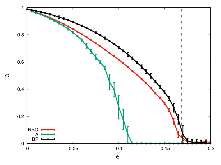
Figure 3: Performance, in terms of the overlap $Q$ (11), of the spectral detection on the assortative HSBM through the non-backtracking matrix (NBO) compared to spectral detection with the adjacency matrix (A) and Bayesian belief propagation (BP). The size of the graph is $N=300000$ for the three curves and averages are taken over $5$ samples. The vertical dashed line marks the detectability transition.

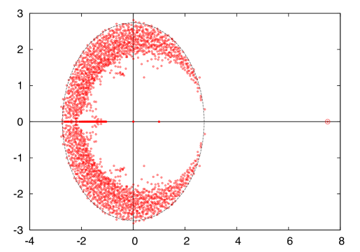
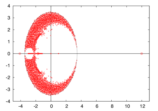
(a) (b) (c)

Figure 4: (a,b) The spectrum of the hypergraph non-backtracking matrix (1) for a hypergraph of size $N=2000$ generated through the planted $2$-in-$4$-sat ($k=4$, $q=2$) for (a) $c=2.5$ and (b) $c=4$. In (b) the informative eigenvalue lie outside the bulk on the left because the model is disassortative. In (c) the spectrum of the adjacency matrix for $c=4$. The informative eigenvalue is hidden in the bulk.

VI-B Planted $2$-in-$4$-sat

In the planted $2$-in-$4$-sat problem, after giving a random binary assignment to the vertices of the network, hyperedges are thrown at random between groups of $k=4$ vertices with a certain non-zero probability only if in the $k$-uplet there is an equal number of zeros and ones. At fixed expected degree $c$, this generative process fits into our general formulation with

$$\begin{split}c_{0011}&=16c\,,\\ c_{\rm in}&=2c\,,\\ c_{\rm out}&=4c\,.\end{split}$$ (52)

This problem has been studied through the cavity method in the so called “locked” case in [24]. Here we are interested in the problem of finding a configuration correlated to the planted one. The scenario is quite different with respect to the preceding case. In fact here we find two phase transitions in the average degree, namely one from an impossible to hard detection [6, 24], and a second one from hard to easy detection that is our main focus. In the hard phase we conjecture that no known algorithm is able to retrieve the planted assignment due to the presence of the stable factorized fixed point, despite the fact that the global fixed point would be the one at high overlap. In this case the hard/easy phase transition in belief propagation is discontinuous and the transition is located at

$$c_{c}=3\,,$$ (53)

which is obtained by plugging (52) into (46). In this case the computation of the effective field in the belief propagation equations is reduced to linear time with

$$h_{a}\simeq\frac{8c}{N^{3}}\,\left(\sum_{i=1}^{N}\chi_{a}^{i}\right)\left(\sum_{i=1}^{N}\chi_{1-a}^{i}\right)^{2}+O\left(\frac{1}{N}\right)\,.$$ (54)

Since this planted problem is essentially disassortative, as shown in Fig. 4 the informative eigenvalue sticks out at the left of the spectrum.

In Fig. 5 we show the performance of the spectral algorithm based on the generalized non-backtracking matrix compared with spectral clustering on the adjacency matrix and with belief propagation. The adjacency matrix displays a terrible behavior up to very large average degree. The non-backtracking matrix instead undergoes a phase transition, located at the same value of the one we encounter in belief-propagation but the transition is continuous. Despite the fact that the non-backtracking operator performs considerably worse than belief propagation, the important point to underline is that the spectral method is completely non-parametric and we do not even need to know what the kernel is. In fact, we can think of the spectral method also as a way to learn the kernel, in order to feed it as a starting condition for the hyper-parameters in belief propagation with parameter learning. Let us take as an example a graph generated with $c=3.4$ and $N=40000$, after running the spectral detection we have an inferred labeling of each vertex. Then let us take the list of $M=34000$ factors and look at their composition (according to the inferred labels). The result is shown in Table I, telling us that we are likely observing a planted $2$-in-$4$-sat model or something very close to it.

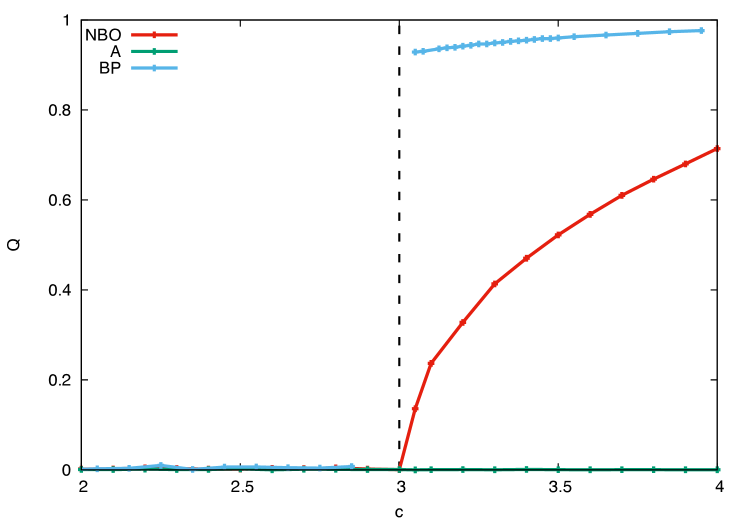
Figure 5: Performance, in terms of the overlap $Q$ (11), of the spectral detection on the planted $2$-in-$4$-sat through the non-backtracking matrix (NBO) compared to spectral detection with the adjacency matrix (A) and Bayesian belief propagation (BP). The size of the graph is $N=200000$ for belief propagation and $N=400000$ for the spectral algorithms. In both cases a single sample was taken. The vertical dashed line marks the hard/easy transition. The adjacency matrix starts giving a non-zero overlap only at very high average degree, namely around $c\approx 9$ which is out of the plot range.

TABLE I: 2-in-4 kernel estimation

0000	1/34000
0001	5764/34000
0011	21758/34000
0111	6477/34000
1111	0/34000

VII Conclusion

In this paper we have proposed a spectral algorithm to detect hidden planted configurations in very sparse hypergraphs, based on a generalization of the non-backtracking Hashimoto matrix. To test the performance of the algorithm we have focused on a generative probabilistic model for hypergraphs in which the hyperedges depend on the incident variables via a fixed probability kernel. Given the generative model, we have also derived an asymptotically (conjectured) optimal belief propagation algorithm and presented a derivation of the non-backtracking matrix as a linearization of belief propagation equations around the factorized fixed point. In addition we have used belief propagation to compute the location of the detectability phase-transition.

The generative model that we consider includes a broad class of problems. Among them we have studied the assortative stochastic block model and the planted $2$-in-$4$-sat. In the first case we obtained that the spectral non-backtracking clustering has a performance that is very close to the optimal belief propagation and displays a detectability phase transition at the same point. It also performed much better than the spectral clustering based on the adjacency matrix that breaks down way before the phase transition due to the sparsity of the graph. In the second case of the planted $2$-in-$4$-sat we observed a different phenomenon, reminiscent of a first order phase transition. While for belief propagation the phase transition is discontinuous from a hard inference phase to an easy inference phase with the overlap that jumps from zero to a value close to one, in the spectral detection algorithm we observe a continuous transition at the very same point. Spectral detection with the adjacency matrix, again, performs badly up to even higher degree. In both cases, the gain provided by the non-backtracking approach was clear.

We also showed that despite the fact that the accuracy of the spectral method is significantly worse w.r.t. belief propagation (although they start to detect assignments at the same values of the parameters), the spectral approach has many important advantages: not only it is entirely non-parametric, but it is also a powerful instrument to learn the parameters, such as the kernel, when they are unknown.

References

- [1] Paul W. Holland, Kathryn Blackmond Laskey, and Samuel Leinhardt. Stochastic blockmodels: First steps. Social Networks, 5(2):109 – 137, 1983.
- [2] Yuchung J. Wang and George Y. Wong. Stochastic blockmodels for directed graphs. Journal of the American Statistical Association, 82(397):8–19, 1987.
- [3] Ulrike von Luxburg. A tutorial on spectral clustering. Statistics and Computing, 17(4):395–416, 2007.
- [4] Aurelien Decelle, Florent Krzakala, Cristopher Moore, and Lenka Zdeborová. Inference and phase transitions in the detection of modules in sparse networks. Phys. Rev. Lett., 107:065701, Aug 2011.
- [5] A. Decelle, F. Krzakala, C. Moore, and L. Zdeborová. Asymptotic analysis of the stochastic block model for modular networks and its algorithmic applications. Phys. Rev. E, 84:066106, 2011.
- [6] Lenka Zdeborová and Florent Krzakala. Quiet planting in the locked constraint satisfaction problems. SIAM Journal on Discrete Mathematics, 25(2):750–770, 2011.
- [7] Peter J. Bickel and Aiyou Chen. A nonparametric view of network models and newman–girvan and other modularities. Proceedings of the National Academy of Sciences, 106(50):21068–21073, 2009.
- [8] A. Coja-Oghlan, E. Mossel, and D. Vilenchik. A spectral approach to analysing belief propagation for 3-colouring. Combinatorics, Probability and Computing, 18:881–912, 11 2009.
- [9] A. Coja-Oghlan. Graph partitioning via adaptive spectral techniques. Combinatorics, Probability and Computing, 19:227–284.
- [10] F. McSherry. Spectral partitioning of random graphs. In Foundations of Computer Science, 2001. Proceedings. 42nd IEEE Symposium on, pages 529–537, Oct 2001.
- [11] Raj Rao Nadakuditi and M. E. J. Newman. Graph spectra and the detectability of community structure in networks. Phys. Rev. Lett., 108:188701, May 2012.
- [12] D. Ghoshdastidar and A. Dukkipati. Consistency of spectral partitioning of uniform hypergraphs under planted partition model. In Z. Ghahramani, M. Welling, C. Cortes, N.D. Lawrence, and K.Q. Weinberger, editors, Advances in Neural Information Processing Systems 27, pages 397–405. Curran Associates, Inc., 2014.
- [13] Dengyong Zhou, Jiayuan Huang, and Bernhard Schölkopf. Learning with hypergraphs: Clustering, classification, and embedding. In B. Schölkopf, J.C. Platt, and T. Hoffman, editors, Advances in Neural Information Processing Systems 19, pages 1601–1608. MIT Press, 2007.
- [14] S. Agarwal, Jongwoo Lim, L. Zelnik-Manor, P. Perona, D. Kriegman, and S. Belongie. Beyond pairwise clustering. In Computer Vision and Pattern Recognition, 2005. CVPR 2005. IEEE Computer Society Conference on, volume 2, pages 838–845 vol. 2, June 2005.
- [15] F. Krzakala, C. Moore, E. Mossel, J. Neeman, A. Sly, L. Zdeborová, and P. Zhang. Spectral redemption in clustering sparse networks. Proceedings of the National Academy of Sciences, 110(52):20935–20940, 2013.
- [16] K. Hashimoto. Zeta functions of finite graphs and representations of p-adic groups automorphic forms and geometry of arithmetic varieties. pages 211–280, 1989.
- [17] E. Abbe and A. Montanari. Conditional random fields, planted constraint satisfaction and entropy concentration. In Prasad Raghavendra, Sofya Raskhodnikova, Klaus Jansen, and JoséD.P. Rolim, editors, Approximation, Randomization, and Combinatorial Optimization. Algorithms and Techniques, volume 8096 of Lecture Notes in Computer Science, pages 332–346. Springer Berlin Heidelberg, 2013.
- [18] Dimitris Achlioptas and Amin Coja-Oghlan. Algorithmic barriers from phase transitions. In Foundations of Computer Science, 2008. FOCS’08. IEEE 49th Annual IEEE Symposium on, pages 793–802. IEEE, 2008.
- [19] Florent Krzakala and Lenka Zdeborová. Hiding quiet solutions in random constraint satisfaction problems. Phys. Rev. Lett., 102:238701, 2009.
- [20] Florent Krzakala, Marc Mézard, and Lenka Zdeborová. Reweighted belief propagation and quiet planting for random k-sat. Journal on Satisfiability, Boolean Modeling and Computation, 8:149–171, 2014.
- [21] Vitaly Feldman, Will Perkins, and Santosh Vempala. Subsampled power iteration: a new algorithm for block models and planted csp’s. arXiv preprint arXiv:1407.2774, 2014.
- [22] C. Bordenave, M. Lelarge, and L. Massoulié. Non-backtracking spectrum of random graphs: community detection and non-regular ramanujan graphs. arXiv:1501.06087v1, 2015.
- [23] M. Mézard and A. Montanari. Information, Physics, and Computation. Oxford Press, Oxford, 2009.
- [24] L. Zdeborová and M. Mézard. Constraint satisfaction problems with isolated solutions are hard. Journal of Statistical Mechanics: Theory and Experiment, 2008(12):P12004, 2008.