Van der Waals Interactions among Alkali Rydberg Atoms with Excitonic States

Abstract

We investigate the influence of the appearance of excitonic states on van der Waals interactions among two Rydberg atoms. The atoms are assumed to be in different Rydberg states, e.g., in the $|ns\rangle$ and $|np\rangle$ states. The resonant dipole-dipole interactions yield symmetric and antisymmetric excitons, with energy splitting that give rise to new resonances as the atoms approach each other. Only far from these resonances the van der Waals coefficients, $C_{6}^{sp}$, can be defined. We calculate the $C_{6}$ coefficients for alkali atoms and present the results for lithium by applying perturbation theory. At short interatomic distances of several $\mu m$, we show that the widely used simple model of two-level systems for excitons in Rydberg atoms breaks down, and the correct representation implies multi-level atoms. Even though, at larger distances one can keep the two-level systems but in including van der Waals interactions among the atoms.

I Introduction

Rydberg atoms, i.e. atoms with large principal quantum numbers $n\gg 1$, have been the subject of extensive research due to their unique optical and electrical features Gallagher (1994). They are an ideal platform for the study of a wide range of quantum phenomena, mainly since their properties scale strongly with $n$, and often turning them extraordinary relative to those of ground-state atoms. The property which has stimulated the most recent experimental and theoretical work is strong interactions among Rydberg atoms that are separated by relatively large distances of several $\mu m$ Saffman et al. (2010); Löw et al. (2012); Jaksch et al. (2000); Lukin et al. (2001); Pohl et al. (2010); Kiffner et al. (2013).

On the other hand, electronic excitations can be delocalized among distant atoms through resonant dipole-dipole interactions to form collective electronic excitations that are termed excitons Davydov (1971); Agranovich (2009). Different processes of resonant energy transfer are possible Gallagher and Pillet (2008), here we concentrate on the exchange type, e.g. $ns\ +\ np\ \leftrightarrow\ np\ +\ ns$. Excitons have been introduced to a system of ultracold atoms in an optical lattice with lowest excited states where van der Waals interactions are negligible Zoubi and Ritsch (2007, 2013). The formation of excitons in a cluster of Rydberg atoms has been investigated, but van der Waals forces were completely neglected and the discussion limited to two-level atoms Wüster et al. (2010); Möbius et al. (2011); Ates et al. (2008). In previous work we investigated the influence of van der Waals interactions on the formation of excitons in an aggregate of two-level Rydberg atoms Zoubi et al. (2014). Coherent energy transfer among Rydberg atoms that induces by resonant dipole-dipole interaction has been realized experimentally at large interatomic distances of tenths $\mu m$ where van der Waals forces are negligible Ravets et al. (2014); Barredo et al. (2015).

An excitonic state contains at least two different atomic states. The simplest case is of two atoms in which one in the $|ns\rangle$ state and the other in the $|np\rangle$ state. The discussion can be limited to dipole-dipole interactions, where dipole-quadrupole, quadrupole-quadrupole and higher order interactions are neglected. Approximate long-range potentials can be derived by applying perturbation theory up to the second order in the dipole-dipole interactions. The lowest order term of the perturbation series results in resonant dipole-dipole interaction of the form $C_{3}^{sp}/R^{3}$, where $R$ is the interatomic distance with the resonant dipole-dipole coefficient $C_{3}^{sp}$. This interaction leads to a coherent mixing of the two possible states, which are $|ns,np\rangle$ and $|np,ns\rangle$. The second order term is of the van der Waals type of the form $C_{6}^{sp}/R^{6}$, with the van der Waals coefficient $C_{6}^{sp}$. As was shown in our previous work Zoubi et al. (2014), van der Waals interactions result in energy shifts that significantly influence the formation of excitons when atoms approach each other. Higher order terms play significant roles and can change completely the long-range interaction potentials Boisseau et al. (2002); Porsev et al. (2014). Furthermore, the appearance of resonances breaks down the validity of the perturbative calculation and then other techniques are required, e.g. in using direct Hamiltonian diagonalization Schwettmann et al. (2006). Moreover, non-adiabatic interactions between Rydberg atoms in different electronic surfaces can be important Robicheaux et al. (2004).

Long-range van der Waals interactions among pairs of Rydberg atoms have been intensively investigated, mainly using a perturbative approach Singer et al. (2005); Reinhard et al. (2007); Béguin et al. (2013). The dispersion coefficients of the type $C_{6}^{ss}$, $C_{6}^{pp}$ and $C_{6}^{dd}$, are calculated and listed for homonuclear dimers of alkali metal atoms in the $ns-ns$, $np-np$ and $nd-nd$ states, where both atoms are in the same state. These coefficients are of importance for experimental and theoretical applications in strongly interacting Rydberg gases, especially for the current cold and ultracold Rydberg atom experiments, e.g., in the implementation of dipole blockade phenomena for quantum information processing Saffman et al. (2010); Löw et al. (2012); Weimer et al. (2010). But coefficients of the mixed type in which atoms are in different electronic states, e.g., $C_{6}^{sp}$, are not much emphasized, while they are of importance for processes that involve resonant energy transfer Zoubi et al. (2014).

In the present paper we study the influence of the formation of excitons on van der Waals interactions among Rydberg atoms. We check the validity of using the simple model of two-level systems to describe excitons in interacting Rydberg atoms. We start by developing simple models using three and four atomic levels that provide a qualitative understanding of the different interactions among Rydberg atoms. In treating $ns-ns$ and $np-np$ Rydberg atoms we extract the limit in which atom-atom interactions have the forms $C_{6}^{ss}/R^{6}$ and $C_{6}^{pp}/R^{6}$. For the case of $ns-np$ Rydberg atoms we derive the condition in which the interactions can be described by $C_{3}^{sp}/R^{3}$ and $C_{6}^{sp}/R^{6}$ terms. Afterwards, we exploit perturbation theory in order to get quantitative values for all $C_{3}$ and $C_{6}$ coefficients by summing over all the allowed atomic states. We treat Rydberg alkali metal atoms, and as an example we present the values for lithium atoms.

We emphasize here van der Waals interactions of the mixed type with coefficient $C_{6}^{sp}$, and examine the effect of resonant dipole-dipole transfer on van der Waals interactions. The point is that as the two states $|ns,np\rangle$ and $|np,ns\rangle$ are degenerate, perturbation theory implies the removal of these degeneracy. But the states are coupled by resonant dipole-dipole interactions and the diagonalization mixes and splits them to yield symmetric and antisymmetric orthogonal states. Then we use these orthogonal states as the zero order eigenstates in the perturbative calculation of the van der Waals interactions. We found that as the symmetric-antisymmetric splitting energy is $R$-dependent new resonances appear as the interatomic distance decreases.

The paper is organized as follows. In section 2 we present a qualitative study of van der Waals interactions among two Rydberg atoms using multi-level simple models. Quantitative derivations of van der Waals interactions appear in section 3 using perturbation theory. Section 4 contains calculations of van der Waals coefficients for alkali Rydberg atoms, and the results are presented for lithium atoms in section 5. A summary is given in section 6. The appendix includes the angular parts of the dipole moment matrix elements.

II Rydberg Atom Interactions: Simple Models

We start by treating Rydberg atoms using models of two, three and four-level systems. The derivations provide a qualitative understanding of the type of interactions that can appear among Rydberg atoms and pave the way towards the quantitative treatment presented in the next section. We examine the validity of using two-level systems for describing excitons in Rydberg atoms. The model of two-level systems is widely used to describe Frenkel excitons in organic solids involving lowest excited states where van der Waals interactions result in small energy shifts Davydov (1971); Agranovich (2009). But for Rydberg atoms van der Waals forces are significant and the appearance of resonances is probable. Hence we examine the validity of using the simple model of two-level systems for Rydberg atoms. Our objective in this section is to extend the simple model into multi-level systems, which are necessary in order to exploit the appearance of resonances. We show that far from resonances one can keep the simple model but in including energy shifts due to van der Waals interactions, which implies quantitative calculations of the van der Waals coefficients that we calculate in the next section using perturbation theory.

II.1 Two atoms in the same Rydberg state

Let us assume the two atoms to be in the same internal atomic level, say in the $(nl)$ state. The two-atom state is $|\pi\rangle=|nl,nl\rangle$ of energy $E_{i}=2E_{nl}$. We assume a single channel to be close to resonance with this state. Namely, we consider a process of the transfer type $nl+nl\leftrightarrow n^{\prime}l^{\prime}+n^{\prime\prime}l^{\prime\prime}$. We have two possible degenerate final states $|\rho_{1}\rangle=|n^{\prime}l^{\prime},n^{\prime\prime}l^{\prime\prime}\rangle$ and $|\rho_{2}\rangle=|n^{\prime\prime}l^{\prime\prime},n^{\prime}l^{\prime}\rangle$, with the energy $E_{f}=E_{n^{\prime}l^{\prime}}+E_{n^{\prime\prime}l^{\prime\prime}}$. The states have the energy detuning $\Delta=E_{f}-E_{i}=E_{n^{\prime}l^{\prime}}+E_{n^{\prime\prime}l^{\prime\prime}}-2E_{nl}$. We assume here coupling among the $|\pi\rangle$ state and each one of the $|\rho_{1}\rangle$ and $|\rho_{2}\rangle$ states, with the coupling parameter $J$, which we specify later. We neglect coupling among the $|\rho_{1}\rangle$ and $|\rho_{2}\rangle$ states. The Hamiltonian that is restricted to the states defined above can be written as

$$H = E_{i}\ |\pi\rangle\langle\pi|+E_{f}\left(|\rho_{1}\rangle\langle\rho_{1}|+|\rho_{2}\rangle\langle\rho_{2}|\right)$$ (1)

$$+ J\left(|\pi\rangle\langle\rho_{1}|+|\pi\rangle\langle\rho_{2}|+|\rho_{1}\rangle\langle\pi|+|\rho_{2}\rangle\langle\pi|\right).$$

In matrix elements we have

$$H=E_{i}\hat{\bf 1}+\left(\begin{tabular}[]{cccc}$0$&$J$&$J$\\ $J$&$\Delta$&$0$\\ $J$&$0$&$\Delta$\\ \end{tabular}\right).$$ (5)

We diagonalize the matrix to get the characteristic equation $(\lambda-\Delta)\left(\lambda^{2}-\lambda\Delta-2J^{2}\right)=0$, with the three solutions

$$\lambda_{1}=\frac{\Delta}{2}-\frac{1}{2}\sqrt{\Delta^{2}+8J^{2}},\ \lambda_{2}=\frac{\Delta}{2}+\frac{1}{2}\sqrt{\Delta^{2}+8J^{2}},\ \lambda_{3}=\Delta.$$ (6)

In the far off-resonant limit, that is $\Delta\gg J$, we get

$$E_{1}\approx E_{i}-2\frac{J^{2}}{\Delta},\ E_{2}\approx E_{f}+2\frac{J^{2}}{\Delta},\ E_{3}=E_{f}.$$ (7)

Transfer processes are induced by resonant dipole-dipole interaction that have the form $J=-\frac{hC_{3}}{R^{3}}$, where $R$ is the interatomic distance, and $C_{3}$ will be calculated in details later. We can also define $D=-2\frac{(hC_{3})^{2}}{\Delta}\frac{1}{R^{6}}$, which is of the van der Waals type. In the general case we have $D=-\frac{hC_{6}}{R^{6}}$, where one need to calculate the van der Waals coefficient $C_{6}$ for each specific states by considering all possible atomic transitions, which is the main aim in the next sections. Next we consider the case of $(ns)$ state in details.

In the case of $|\pi\rangle=|ns,ns\rangle$ of energy $E_{i}=2E_{ns}$, we have, e.g., the channel $ns+ns\leftrightarrow np+(n-1)p$, that is $|\rho_{1}\rangle=|np,(n-1)p\rangle$ and $|\rho_{2}\rangle=|(n-1)p,np\rangle$, with the energy $E_{f}=E_{np}+E_{(n-1)p}$, and with the detuning $\Delta_{ss}=E_{np}+E_{(n-1)p}-2E_{ns}$, (see Fig. 1). The energy of the two interacting atoms is $E_{ss}=2E_{ns}+D_{ss}$, with the van der Waals interaction $D_{ss}=-2\frac{\left(hC_{3}^{ss}\right)^{2}}{\Delta_{ss}}\frac{1}{R^{6}}$. In the general case we can write $D_{ss}=-\frac{hC^{ss}_{6}}{R^{6}}$. Later on we calculate the $C_{3}^{ss}$ and $C^{ss}_{6}$ coefficients in details. Similar consideration holds for the case of two $(np)$-state atoms.

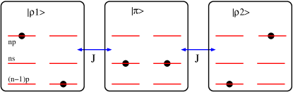
Figure 1: The three states $|\pi\rangle$, $|\rho_{1}\rangle$, and $|\rho_{2}\rangle$ are illustrated, with the coupling among them.

II.2 Two atoms in different Rydberg states

Here we consider the case in which the atoms are in different states, e.g., one atom in the $(ns)$-state and the other in $(np)$-state. We get two degenerate states $|\pi_{1}\rangle=|np,ns\rangle$ and $|\pi_{2}\rangle=|ns,np\rangle$ of energy $E_{i}=E_{ns}+E_{np}$. We have, e.g., the possible transfer channel of $ns+np\leftrightarrow(n-1)p+(n+1)s$. Further, we consider the two degenerate states $|\rho_{1}\rangle=|(n+1)s,(n-1)p\rangle$ and $|\rho_{2}\rangle=|(n-1)p,(n+1)s\rangle$, of energy $E_{f}=E_{(n+1)s}+E_{(n-1)p}$, (see Fig. 2). Their energy detuning compared to $|\pi\rangle$ state is $\Delta_{sp}=E_{(n+1)s}-E_{ns}+E_{(n-1)p}-E_{np}$. The states $|\pi_{1}\rangle=|np,ns\rangle$ and $|\pi_{2}\rangle=|ns,np\rangle$ are coupled by the resonant dipole-dipole interaction of strength $J$, where $J=-\frac{hC_{3}^{sp}}{R^{3}}$. The state $|\pi_{1}\rangle=|np,ns\rangle$ is coupled to $|\rho_{1}\rangle=|(n+1)s,(n-1)p\rangle$ by the resonant dipole-dipole interaction of strength $J^{\prime}$, and the state $|\pi_{2}\rangle=|ns,np\rangle$ is coupled to $|\rho_{2}\rangle=|(n-1)p,(n+1)s\rangle$ with the same parameter $J^{\prime}$. We neglect the resonant dipole-dipole interaction among the $|\rho_{1}\rangle=|(n+1)s,(n-1)p\rangle$ and $|\rho_{2}\rangle=|(n-1)p,(n+1)s\rangle$ states, due to their small amplitudes.

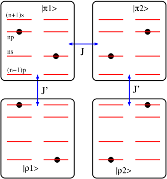
Figure 2: The four states $|\pi_{1}\rangle$, $|\pi_{2}\rangle$, $|\rho_{1}\rangle$, and $|\rho_{2}\rangle$ are illustrated, with the coupling among them.

The Hamiltonian can be then written as

$$H = E_{i}\left(|\pi_{1}\rangle\langle\pi_{1}|+|\pi_{2}\rangle\langle\pi_{2}|\right)+E_{f}\left(|\rho_{1}\rangle\langle\rho_{1}|+|\rho_{2}\rangle\langle\rho_{2}|\right)$$ (8)

$$+ J\left(|\pi_{1}\rangle\langle\pi_{2}|+|\pi_{2}\rangle\langle\pi_{1}|\right)$$

$$+ J^{\prime}\left(|\pi_{1}\rangle\langle\rho_{1}|+|\pi_{2}\rangle\langle\rho_{2}|+|\rho_{1}\rangle\langle\pi_{1}|+|\rho_{2}\rangle\langle\pi_{2}|\right).$$

In matrix elements we get

$$H=E_{i}\hat{\bf 1}+\left(\begin{tabular}[]{cccc}$0$&$J$&$J^{\prime}$&$0$\\ $J$&$0$&$0$&$J^{\prime}$\\ $J^{\prime}$&$0$&$\Delta_{sp}$&$0$\\ $0$&$J^{\prime}$&$0$&$\Delta_{sp}$\\ \end{tabular}\right).$$ (13)

We diagonalize the Hamiltonian, to get the characteristic equations

$$\left(\lambda-\Delta_{sp}\right)^{2}\left(\lambda^{2}-J^{2}\right)-2\lambda\left(\lambda-\Delta_{sp}\right)J^{\prime\ 2}+J^{\prime\ 4}=0,$$ (14)

with the four solutions

$$\lambda_{1,2} = \frac{\Delta_{sp}\mp J}{2}-\frac{1}{2}\sqrt{\left(\Delta_{sp}\pm J\right)^{2}+4J^{\prime\ 2}},$$

$$\lambda_{3,4} = \frac{\Delta_{sp}\mp J}{2}+\frac{1}{2}\sqrt{\left(\Delta_{sp}\pm J\right)^{2}+4J^{\prime\ 2}}.$$ (15)

In the far off-resonant limit, that is $\Delta_{sp}\gg J^{\prime}$, we get the energies

$$E_{a,b} = E_{ns}+E_{np}\mp J-\frac{J^{\prime\ 2}}{\Delta_{sp}\pm J},$$

$$E_{c,d} = E_{(n+1)s}+E_{(n-1)p}+\frac{J^{\prime\ 2}}{\Delta_{sp}\pm J}.$$ (16)

As far as $\Delta_{sp}\gg J$ the shifts are of the van der Waals type, where $D_{sp}=-J^{\prime\ 2}/\Delta_{sp}$. In general we can write $D_{sp}=-\frac{hC_{6}^{sp}}{R^{6}}$, where the $C_{6}$ coefficient will be calculated later.

II.3 Two-level atoms

In the light of this result, we can go one step back and start with two effective two-level atoms including van der Waals interactions. We again treat the case of one atom in the $(ns)$ Rydberg state, and the other in the $(np)$ state, as seen in Fig. 3. The atoms are separated by the distance $R$. We have two states $|\pi_{1}\rangle=|np,ns\rangle$ and $|\pi_{2}\rangle=|ns,np\rangle$, and they are degenerate with the energy $E_{0}=E_{ns}+E_{np}+D_{sp}$, where we include the van der Waals interaction among the two atoms $D_{sp}=-hC_{6}^{sp}/R^{6}$. The energy transfer parameter among the two states is as before $J=-hC_{3}^{sp}/R^{3}$. These consideration exactly fits with the above four-level model in the limit of $\Delta_{sp}\gg J$, where the detuning $\Delta_{sp}$ is much larger than the symmetric-antisymmetric splitting.

The Hamiltonian is now written as

$$H=E_{0}\left(|\pi_{1}\rangle\langle\pi_{1}|+|\pi_{2}\rangle\langle\pi_{2}|\right)+J\left(|\pi_{1}\rangle\langle\pi_{2}|+|\pi_{2}\rangle\langle\pi_{1}|\right).$$ (17)

The Hamiltonian can be diagonalized by using the collective states

$$|\psi_{a}\rangle=\frac{|\pi_{1}\rangle+|\pi_{2}\rangle}{\sqrt{2}},\ |\psi_{b}\rangle=\frac{|\pi_{1}\rangle-|\pi_{2}\rangle}{\sqrt{2}},$$ (18)

which gives

$$H=E_{a}\ |\psi_{a}\rangle\langle\psi_{a}|+E_{b}\ |\psi_{b}\rangle\langle\psi_{b}|,$$ (19)

with the energies $E_{a}=E_{0}+J$ and $E_{b}=E_{0}-J$, which fit exactly with the above derived energies.

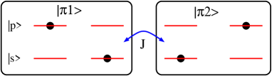
Figure 3: The two states $|\pi_{1}\rangle$ and $|\pi_{2}\rangle$ are illustrated with the coupling $J$ among them.

As other states can be close to resonance with the considered states, the picture of two-level atoms breaks down at short interatomic distances of several $\mu m$. Then, the excitonic picture implies multi-level systems, as beside the considered states, e.g. $ns$ and $np$, the formalism must include all close to resonance states, e.g $(n+1)s$ and $(n-1)p$, as treated before. The model of two-level systems can be reserved for larger interatomic distances when other states are off-resonance, but in including van der Waals interactions among the atoms. We adopted this direction in treating $N$ Rydberg atoms in our previous paper Zoubi et al. (2014). At much larger interatomic distances of tenth of $\mu m$ the van der Waals interactions are negligible.

After this qualitative study of the resonant dipole-dipole and van der Waals interactions, we move to quantitative calculations of the different $C_{3}$ and $C_{6}$ coefficients.

III Dimeric Energies in Perturbation Theory

We give first a general presentation of a perturbative treatment for the electrostatic interactions among Rydberg atoms. For a system of two atoms the Hamiltonian reads $\hat{H}=\hat{H}_{1}+\hat{H}_{2}+\hat{V}$, where $\hat{H}_{\alpha}$ is the $\alpha$ independent atom Hamiltonian, and $\hat{V}$ is the interaction among the two atoms. We assume the independent atom eigenstates to be known and given by $\hat{H}_{\alpha}|\phi_{\alpha}^{i}\rangle=E_{\alpha}^{i}|\phi_{\alpha}^{i}\rangle$, where the eigenstates are orthonormal with $\langle\phi_{\beta}^{j}|\phi_{\alpha}^{i}\rangle=\delta_{\alpha\beta}\delta_{ij}$, and $\sum_{i}|\phi_{\alpha}^{i}\rangle\langle\phi_{\alpha}^{i}|=\hat{\bf 1}$.

The lowest order interaction among neutral atoms is the dipole-dipole one, where

$$\hat{V}=\frac{1}{4\pi\epsilon_{0}R^{3}}\left\{\left(\hat{\mbox{\boldmath$\mu$}}_{1}\cdot\hat{\mbox{\boldmath$\mu$}}_{2}\right)-3\frac{\left(\hat{\mbox{\boldmath$\mu$}}_{1}\cdot{\bf R}\right)\left(\hat{\mbox{\boldmath$\mu$}}_{2}\cdot{\bf R}\right)}{R^{5}}\right\},$$ (20)

with ${\bf R}={\bf R}_{1}-{\bf R}_{2}$, and the interatomic distance is $R=|{\bf R}|$. Here $\hat{\mbox{\boldmath$\mu$}}_{\alpha}$ is the dipole operator at atom $\alpha$. We assume no permanent dipoles to exist, and hence $\mbox{\boldmath$\mu$}_{\alpha}^{ii}=\langle\phi_{\alpha}^{i}|\hat{\mbox{\boldmath$\mu$}}_{\alpha}|\phi_{\alpha}^{i}\rangle=0$. We have $\mbox{\boldmath$\mu$}_{\alpha}^{ij}=\langle\phi_{\alpha}^{i}|\hat{\mbox{\boldmath$\mu$}}_{\alpha}|\phi_{\alpha}^{j}\rangle$ with $(i\neq j)$. The atoms are taken to be localized along the $z$-axis, which is also the quantization axis, hence

$$\hat{V}=\frac{1}{4\pi\epsilon_{0}R^{3}}\left\{\hat{\mu}_{1x}\hat{\mu}_{2x}+\hat{\mu}_{1y}\hat{\mu}_{2y}-2\hat{\mu}_{1z}\hat{\mu}_{2z}\right\}.$$ (21)

We apply perturbation theory in order to calculate the resonant dipole-dipole and van der Waals coefficients by deriving the corrections to each dimer energy.

We write the perturbative terms up to the second order explicitly where the two atoms are assumed to be in the states $i$ and $j$. The lowest order correction to the free energy is $J^{ij,kl}=\langle\phi_{1}^{i},\phi_{2}^{j}|\hat{V}|\phi_{1}^{k},\phi_{2}^{l}\rangle$, where for the dimer we use a product basis $|\phi_{1}^{i},\phi_{2}^{j}\rangle=|\phi_{1}^{i}\rangle|\phi_{2}^{j}\rangle$. This term give rise to resonant dipole-dipole interaction that is responsible for the energy transfer among atoms at different internal states. When the two atoms are in the same $i$-th quantum state one has $\langle\phi_{1}^{i},\phi_{2}^{i}|\hat{V}|\phi_{1}^{i},\phi_{2}^{i}\rangle=0$. Only terms of $(i\neq k)$ and $(j\neq l)$ are nonzero, with the appropriate selection rules. We define $J^{ij,kl}=-\frac{hC_{3}^{ij,kl}}{R^{3}}$, where now

$$C_{3}^{ij,kl}=-\frac{1}{4\pi\epsilon_{0}}\left\{\mu_{1x}^{ik}\mu_{2x}^{jl}+\mu_{1y}^{ik}\mu_{2y}^{jl}-2\mu_{1z}^{ik}\mu_{2z}^{jl}\right\},$$ (22)

and the transition dipole matrix element is defined by $\mu_{\alpha r}^{ij}=\langle\phi_{\alpha}^{i}|\hat{\mu}_{\alpha r}|\phi_{\alpha}^{j}\rangle$, with $(r=x,y,z)$.

Resonances can appear among the dimer states, e.g., for $|\phi_{1}^{i},\phi_{2}^{j}\rangle$ and $|\phi_{1}^{k},\phi_{2}^{l}\rangle$ states with the energy $E_{1}^{k}+E_{2}^{l}=E_{1}^{i}+E_{2}^{j}$, which implies the use of degenerate perturbation theory. In the following we present separately the degenerate and non-degenerate perturbation theory.

III.1 Non-degenerate states

For non degenerate states $|\phi_{1}^{i},\phi_{2}^{j}\rangle$ the first order term $\langle\phi_{1}^{i},\phi_{2}^{j}|\hat{V}|\phi_{1}^{i},\phi_{2}^{j}\rangle$ vanishes, because the atoms do not have a permanent dipole. The second order term is

$$D^{ij}=-\sum_{k,l}\frac{\langle\phi_{1}^{i},\phi_{2}^{j}|\hat{V}|\phi_{1}^{k},\phi_{2}^{l}\rangle\langle\phi_{1}^{k},\phi_{2}^{l}|\hat{V}|\phi_{1}^{i},\phi_{2}^{j}\rangle}{E_{1}^{k}-E_{1}^{i}+E_{2}^{l}-E_{2}^{j}},$$ (23)

which results in van der Waals interactions. Since $\hat{V}$ has a $1/R^{3}$ distance dependence, we can write $D^{ij}=-\frac{hC_{6}^{ij}}{R^{6}}$, where we have defined

$$C_{6}^{ij}=\left(\frac{1}{4\pi\epsilon_{0}}\right)^{2}\sum_{k,l}\frac{\left|\mu_{1x}^{ik}\mu_{2x}^{jl}+\mu_{1y}^{ik}\mu_{2y}^{jl}-2\mu_{1z}^{ik}\mu_{2z}^{jl}\right|^{2}}{E_{1}^{k}-E_{1}^{i}+E_{2}^{l}-E_{2}^{j}}.$$ (24)

The present perturbation theory can break down due to the appearance of resonances at $E_{1}^{k}+E_{2}^{l}=E_{2}^{j}+E_{1}^{i}$, and one appeals to other methods, e.g., to the direct Hamiltonian diagonalization Schwettmann et al. (2006).

III.2 Degenerate States

We now consider states $|\phi_{1}^{i},\phi_{2}^{j}\rangle$ for which a state $|\phi_{1}^{k},\phi_{2}^{l}\rangle$ with the same energy exists, i.e. $E_{i}+E_{j}=E_{k}+E_{l}$, and for which also $J^{ij,kl}=\langle\phi_{1}^{i},\phi_{2}^{j}|\hat{V}|\phi_{1}^{k},\phi_{2}^{l}\rangle\neq 0$. Then we have to use degenerate perturbation theory and first diagonalize the degenerate subspace. Here we concentrate in degenerate states of the type $|\phi_{1}^{i},\phi_{2}^{j}\rangle$ and $|\phi_{1}^{j},\phi_{2}^{i}\rangle$. The ’correct’ zero order states have the form

$$|\phi_{\pm}^{ij}\rangle=|\phi_{1}^{i},\phi_{2}^{j}\rangle\pm|\phi_{1}^{j},\phi_{2}^{i}\rangle,$$ (25)

with energy

$$E_{\pm}^{ij}=E_{1}^{i}+E_{2}^{j}\pm J^{ij}.$$ (26)

The first order contributions then vanish and the second order term, which has a $1/R^{6}$ behavior is calculated by

$$D^{ij}_{\pm}=-\sum_{k,l}\frac{|\langle\phi_{\pm}^{ij}|\hat{V}|\phi^{k}_{1},\phi^{l}_{2}\rangle|^{2}}{E^{k}_{1}+E^{l}_{2}-E_{\pm}^{ij}},$$ (27)

where the sum over $k$ and $l$ includes all states but $|\phi_{\pm}^{ij}\rangle$. Note that resonances appear at $E^{k}_{1}+E^{l}_{2}=E_{\pm}^{ij}$ and then a special treatment is required.

IV Interactions between Alkali Rydberg Atoms

We calculate the $C_{3}$ and $C_{6}$ coefficients for specific cases that include the $|\phi^{ns}\rangle$ and $|\phi^{np}\rangle$ states, and we concentrate in interactions among alkali Rydberg atoms. We use the nondegenerate perturbation theory in order to calculate $C_{6}^{ss}$ and $C_{6}^{pp}$ coefficients. Next we calculate $C_{6}^{sp}$ coefficients, and as here a resonance appears between the states $|\phi_{1}^{ns},\phi_{2}^{np}\rangle$ and $|\phi_{1}^{np},\phi_{2}^{ns}\rangle$ we use degenerate perturbation theory. Let us first present the atomic states for alkali Rydberg atoms.

IV.1 Atomic eigenstates

The atomic state is given by the wave function $\psi_{nlm}(r,\theta,\phi)=R_{nl}(r)Y_{lm}(\theta,\phi)$, where $R_{nl}(r)$ is the radial wavefunction and $Y_{lm}(\theta,\phi)$ is the spherical harmonic function. In general the dipole moment matrix element can be factorized as $\mu_{r}^{nlm,n^{\prime}l^{\prime}m^{\prime}}=e\tilde{\mu}_{r}^{lm,l^{\prime}m^{\prime}}{\cal I}^{nl}_{n^{\prime}l^{\prime}}$, where the radial integral is

$${\cal I}^{nl}_{n^{\prime}l^{\prime}}=\int_{0}^{\infty}dr\ r^{3}R_{n^{\prime}l^{\prime}}R_{nl},$$ (28)

and the angular part is

$$\tilde{\mu}_{i}^{lm,l^{\prime}m^{\prime}}=\int_{0}^{\pi}d\theta\int_{0}^{2\pi}d\phi\sin\theta\ Y^{\ast}_{lm}(\theta,\phi)\hat{\bf e}_{i}Y_{l^{\prime}m^{\prime}}(\theta,\phi).$$ (29)

Here $\hat{\bf e}_{i}$ are the axis unit vectors with

$$\hat{\bf e}_{x}=\sin\theta\cos\phi,\ \hat{\bf e}_{y}=\sin\theta\sin\phi,\ \hat{\bf e}_{z}=\cos\theta.$$ (30)

The radial wave function for alkali atoms in atomic units is given by

$$R_{nl}(r) = \frac{2}{n^{\star 2}}\sqrt{\frac{(n^{\star}-l^{\star}-1)!}{(n^{\star}+l^{\star})!}}$$ (31)

$$\times \left(\frac{2r}{n^{\star}}\right)^{l^{\star}}e^{-r/n^{\star}}L^{2l^{\star}+1}_{n^{\star}-l^{\star}-1}\left(\frac{2r}{n^{\star}}\right),$$

where $n^{\star}=n-\delta_{nl}$ and $l^{\star}=l-\delta_{nl}+I(l)$, with the quantum defect $\delta_{nl}=\delta_{0}^{l}+\frac{\delta_{2}^{l}}{(n-\delta_{0}^{l})^{2}}$, and $I(l)$ is the nearest integer below or equal to $\delta_{nl}$. For the energy we have $E_{nl}=\frac{-1}{2(n-\delta_{nl})^{2}}$. Moreover we neglect fine and hyperfine splitting, which is a good approximation for lithium atoms that we present later.

IV.2 $C_{6}^{ss}$ and $C_{6}^{pp}$ Coefficients

We present here detailed calculations of $C_{6}^{ss}$ and $C_{6}^{pp}$ coefficients for atoms in the $(ns)$ and $(np)$ states. We concentrate on alkali metal atoms excited to Rydberg states and hence we deal with a single electronic state at each atom that is represented by three quantum numbers $(n,l,m)$, where $n=1,2,\cdots$, $l=0,\cdots,n-1$, and $m=-l,\cdots,+l$.

We write the expression for the van de Waals coefficients as follows

$$C_{6}^{ns,ns} = \left(\frac{e^{2}}{4\pi\epsilon_{0}}\right)^{2}A_{ns}^{ns},$$

$$C_{6}^{npm,np\bar{m}} = \left(\frac{e^{2}}{4\pi\epsilon_{0}}\right)^{2}A_{np\bar{m}}^{npm},$$ (32)

where we defined

$$A_{n\bar{l}\bar{m}}^{nlm}=\sum_{n^{\prime}l^{\prime},n^{\prime\prime}l^{\prime\prime}}^{\prime}\left|\wp_{\bar{l}\bar{m},l^{\prime\prime}}^{lm,l^{\prime}}\right|^{2}\frac{|{\cal I}^{nl}_{n^{\prime}l^{\prime}}{\cal I}^{n\bar{l}}_{n^{\prime\prime}l^{\prime\prime}}|^{2}}{\Delta^{nl,n\bar{l}}_{n^{\prime}l^{\prime},n^{\prime\prime}l^{\prime\prime}}},$$ (33)

and the prime over the summation indicates that $nl\neq n^{\prime}l^{\prime}$ and $n\bar{l}\neq n^{\prime\prime}l^{\prime\prime}$. We have

$$\Delta^{nl,n\bar{l}}_{n^{\prime}l^{\prime},n^{\prime\prime}l^{\prime\prime}}=E_{n^{\prime}l^{\prime}}+E_{n^{\prime\prime}l^{\prime\prime}}-E_{nl}-E_{n\bar{l}},$$ (34)

and

$$|\wp_{\bar{l}\bar{m},l^{\prime\prime}}^{lm,l^{\prime}}|^{2} = \sum_{m^{\prime},m^{\prime\prime}}\left|\tilde{\mu}_{x}^{lm,l^{\prime}m^{\prime}}\tilde{\mu}_{x}^{\bar{l}\bar{m},l^{\prime\prime}m^{\prime\prime}}+\tilde{\mu}_{y}^{lm,l^{\prime}m^{\prime}}\tilde{\mu}_{y}^{\bar{l}\bar{m},l^{\prime\prime}m^{\prime\prime}}\right.$$ (35)

$$- \left.2\tilde{\mu}_{z}^{lm,l^{\prime}m^{\prime}}\tilde{\mu}_{z}^{\bar{l}\bar{m},l^{\prime\prime}m^{\prime\prime}}\right|^{2}.$$

As we treat two identical atoms, we dropped the atom index. We calculate the radial parts, ${\cal I}$, of the $A$ parameters numerically, and the angular parts, $\left|\wp\right|^{2}$, are calculated analytically and presented in the appendix.

We aim now to calculate the $C_{3}$ coefficient, which can be written as

$$C_{3}^{s,pm}=\frac{-1}{4\pi\epsilon_{0}}\wp^{s,pm}\left|{\cal I}^{np}_{ns}\right|^{2},$$ (36)

where

$$\wp^{s,pm}=\tilde{\mu}_{x}^{s,pm}\tilde{\mu}_{x}^{pm,s}+\tilde{\mu}_{y}^{s,pm}\tilde{\mu}_{y}^{pm,s}-2\tilde{\mu}_{z}^{s,pm}\tilde{\mu}_{z}^{pm,s},$$ (37)

and here we have $\wp^{s,p0}=-\frac{2}{3}$ and $\wp^{s,p\pm 1}=\frac{1}{3}$.

IV.3 $C_{6}^{sp}$ Coefficients

One needs to be careful when calculating the $C_{6}^{sp}$ coefficients, as the states $|ns,np\rangle$ and $|np,ns\rangle$ are degenerate, and perturbation theory implies the removal of this degeneracy, as we presented before. The two states are coupled by the resonant dipole-dipole interaction, which yields two diagonal states of symmetric and antisymmetric mixing, where these orthogonal states used as the zero order basis for the second order perturbation theory.

The diagonal eigenstates are

$$|\pm\rangle=\frac{|ns,npm\rangle\pm|npm,ns\rangle}{\sqrt{2}},$$ (38)

with the diagonal energies

$$E_{n}^{\pm}(R)=E_{ns}+E_{np}\pm J^{ns,npm}(R),$$ (39)

where

$$J^{ns,npm}(R)=-\frac{hC_{3}^{ns,npm}}{R^{3}}.$$ (40)

The diagonal states have splitting energy of $2J^{ns,npm}(R)$. We aim to calculate

$$D_{\alpha}^{ns,npm} = -\left(\frac{1}{4\pi\epsilon_{0}R^{3}}\right)^{2}$$ (41)

$$\times \sum_{k,l}\frac{\left|\mu_{x}^{\alpha k}\mu_{x}^{\alpha l}+\mu_{y}^{\alpha k}\mu_{y}^{\alpha l}-2\mu_{z}^{\alpha k}\mu_{z}^{\alpha l}\right|^{2}}{E_{k}+E_{l}-E^{\alpha}_{n}(R)},$$

with $(\alpha=\pm)$, $(k=n^{\prime}l^{\prime}m^{\prime})$ and $(l=n^{\prime\prime}l^{\prime\prime}m^{\prime\prime})$.

The calculation yields

$$D_{\pm}^{ns,npm}=-2\left(\frac{e^{2}}{4\pi\epsilon_{0}R^{3}}\right)^{2}$$ (42)

$$\times \sum_{n^{\prime}l^{\prime},n^{\prime\prime}l^{\prime\prime}}^{\prime}\left|\wp_{pm,l^{\prime\prime}}^{s,l^{\prime}}\right|^{2}\frac{|{\cal I}^{ns}_{n^{\prime}l^{\prime}}{\cal I}^{np}_{n^{\prime\prime}l^{\prime\prime}}|^{2}}{\Delta^{ns,np}_{n^{\prime}l^{\prime},n^{\prime\prime}l^{\prime\prime}}\mp J_{n}^{s,pm}(R)}.$$

The $R$ dependence in the denominator through $J_{n}^{s,pm}(R)$ can bring new resonances as atoms approach each other and then the present perturbation theory breaks down. Event hough, far from resonance, that is $\Delta^{ns,np}_{n^{\prime}l^{\prime},n^{\prime\prime}l^{\prime\prime}}\gg J_{n}^{s,pm}(R)$, the $C_{6}^{sp}$ coefficients can be safely defined by $D^{sp}=-hC_{6}^{sp}/R^{6}$, where

$$C_{6}^{ns,np\bar{m}}=\left(\frac{e^{2}}{4\pi\epsilon_{0}}\right)^{2}A_{np\bar{m}}^{ns}.$$ (43)

As before the radial parts are calculated numerically, and the angular parts calculated analytically and presented in the appendix.

V Values for Lithium Atom

We calculate now all $C_{6}$ and $C_{3}$ coefficients for lithium atoms, by using the known defect parameters Lorentzen and Niemax (1983). For $ns$ we have $\delta_{0}^{s}=0.399$ and $\delta_{2}^{s}=0.03$, for $np$ we have $\delta_{0}^{p}=0.0473$ and $\delta_{2}^{p}=-0.026$, and for $nd$ we have $\delta_{0}^{d}=0.002$ and $\delta_{2}^{d}=-0.015$.

Converting the above $A$ parameters to SI units requires the change $A\rightarrow\left(\frac{4\pi\epsilon_{0}a_{0}^{5}}{e^{2}}\right)A$, as we have a factor of $\frac{e^{2}}{4\pi\epsilon_{0}a_{0}}$ from the energy, and a factor of $a_{0}$ from the radial function ${\cal I}$. We obtain $C_{6}^{ns,ns}=BA_{ns}^{ns}$ and $D_{6}^{np\bar{m},npm}=BA_{np\bar{m}}^{npm}$, where $B=\frac{e^{2}a_{0}^{5}}{4\pi\epsilon_{0}}$. Using $\epsilon_{0}\approx 0.0055\ e/(V\AA)$, and $a_{0}\approx 0.53\ \AA$, we get $B\approx 0.6\ eV\AA^{6}$, or $B=h\bar{B}$, with $h\approx 4.135\times 10^{-15}\ eVS$, we get $\bar{B}\approx 1.5\times 10^{-10}\ Hz(\mu m)^{6}$. Moreover, we have $C_{3}^{s,pm}=-F\wp^{s,pm}\left|{\cal I}^{np}_{ns}\right|^{2}$, where $F=\frac{a_{0}^{2}e^{2}}{4\pi\epsilon_{0}}$. We use $F=h\bar{F}$ with $\bar{F}\approx 10^{3}\ Hz(\mu m)^{3}$

We plot now the results for all $C_{6}^{ss}$, $C_{6}^{pp}$ and $C_{3}^{sp}$ coefficients ranging from $n=50$ up to $n=100$. In Fig. 4 we plot $C_{6}^{ss}$, and in Fig. 5 we plot $C_{6}^{p0,p0}$, $C_{6}^{p0,p\pm 1}$ and $C_{6}^{p\pm 1,p\pm 1}$. Here $C_{6}^{ss}$ coefficients are negative that lead to repulsive van der Waals forces, and $C_{6}^{pp}$ are positive that lead to attractive ones. The results for $C_{3}^{s,p0}$ and $C_{3}^{s,p\pm 1}$ are plotted in Fig. 6. $C_{3}^{s,p0}$ coefficients are positive that lead to attractive resonant dipole-dipole interactions, and $C_{3}^{s,p\pm 1}$ are negative that lead to repulsive ones.

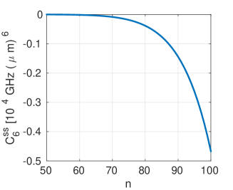
Figure 4: $C_{6}^{ss}$ as a function of $n$ for lithium atoms.

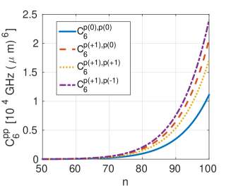
Figure 5: $C_{6}^{p0,p0}$, $C_{6}^{p0,p\pm 1}$ and $C_{6}^{p\pm 1,p\pm 1}$ as a function of $n$ for lithium atoms.

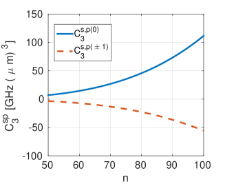
Figure 6: $C_{3}^{s,p0}$, and $C_{6}^{s,p\pm 1}$ as a function of $n$ for lithium atoms.

Now we present the results for $D_{\pm}^{sp}$ energies that derived in using the diagonal states as zero order in perturbation theory for lithium atoms. The main feature of $D_{\pm}^{sp}$ is in their $R$ dependent. We present the plots for different interatomic distances. In Fig. 7 we plot $D_{+}^{s,p0}$ and $D_{-}^{s,p0}$ for $R=7\mu m$, and in Fig. 8 for $R=2\mu m$. It is clear that resonances start to appear at smaller $n$ as atoms approach each other. The $D_{+}^{s,p}$ and $D_{-}^{s,p}$ energies are different due to the symmetric-antisymmetric energy splitting, but for small $n$ as the splitting is much smaller than the energy detuning then the coefficients become equal, and in this limit one can define $C_{6}^{sp}$ coefficients. In Fig. 9 we plot $C_{6}^{s,p(0)}$ and $C_{6}^{s,p(\pm 1)}$ coefficients from $(n=20)$ up to $(n=70)$. In this region no resonances appear down to small interatomic distances of $2\ \mu m$, as it is clear from the above plots. Here the $C_{6}^{s,p(0)}$ coefficients are negative for $n>30$ and then the van der Waals interaction is repulsive, but the $C_{6}^{s,p(\pm 1)}$ coefficients are positive and the interaction is attractive.

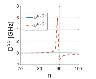
Figure 7: $D_{+}^{s,p0}$ and $D_{-}^{s,p0}$ as a function of $n$ for $R=7\mu m$ of lithium atoms.

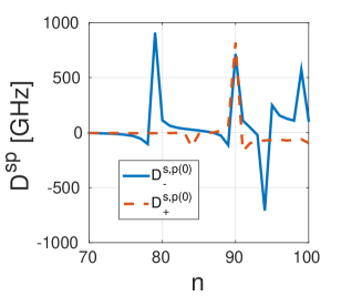
Figure 8: $D_{+}^{s,p0}$ and $D_{-}^{s,p0}$ as a function of $n$ for $R=2\mu m$ of lithium atoms.

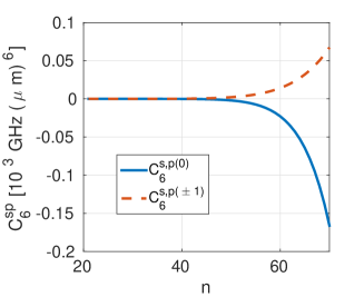
Figure 9: $C_{6}^{s,p(0)}$ and $C_{6}^{s,p(\pm 1)}$ as a function of $n$ for lithium atoms.

VI Conclusions

In summary we investigated van der Waals interactions among two Rydberg atoms for the case where the atoms are in different internal states. For example, we treated in details the case with one atom in the $(ns)$-state and the other in $(np)$-state. The simplest model for achieving a qualitative understanding of the interactions is of four-level atoms, e.g., with $|ns\rangle$, $|np\rangle$, $|n^{\prime}p\rangle$ and $|n^{\prime\prime}s\rangle$ states of energies $E_{ns}$, $E_{np}$, $E_{n^{\prime}p}$ and $E_{n^{\prime\prime}s}$, respectively. The two states $|ns,np\rangle$ and $|np,ns\rangle$ are degenerate and couple by resonant dipole-dipole interaction of the type $J_{sp}=-hC_{3}^{sp}/R^{3}$, which mixes and splits the states to give symmetric and antisymmetric orthogonal ones. We show that van der Waals interaction among the two atoms can be formulated as $D_{sp}=-hC_{6}^{sp}/R^{6}$ in the limit of off-resonance, that is in the limit $|E_{ns}+E_{np}-E_{n^{\prime}p}-E_{n^{\prime\prime}s}|\gg|J_{sp}|$. In this limit the model of two-level atoms is valid, but in including van der Waals interactions.

Next we presented a quantitative calculation of van der Waals coefficients among two alkali Rydberg atoms in considering all allowed electronic states. Due to the resonance among the states $|ns,np\rangle$ and $|np,ns\rangle$ we applied degenerate perturbation theory. The zero order states used in perturbation theory are the orthogonal states $|nsp\rangle_{\pm}=\frac{|ns,np\rangle\pm|np,ns\rangle}{\sqrt{2}}$ with energies $E_{\pm}^{nsp}=E_{ns}+E_{np}\pm J_{nsp}(R)$. We found that due to the symmetric-antisymmetric energy splitting dependence on $R$ new resonances appear when atoms approach each other, and only far from these resonance one can define $C_{6}^{sp}$ coefficients. Moreover, using non-degenerate perturbation theory we calculated all van der Waals coefficients among alkali Rydberg atoms in the same state, mainly for the $|ns,ns\rangle$ and $|np,np\rangle$ states, and we presented the results for lithium atoms.

Appendix A Angular Part of Dipole Moment Matrix Elements

In this appendix we present the angular part calculations of the dipole moment matrix elements. Direct calculations yield the non-zero matrix elements

$$\tilde{\mu}_{x}^{00,1\pm 1}=\frac{\mp 1}{\sqrt{6}} \tilde{\mu}_{x}^{10,2\pm 1}=\frac{\mp 1}{\sqrt{10}},$$ ,

$$\tilde{\mu}_{x}^{1\pm 1,20}=\frac{\pm 1}{\sqrt{30}} \tilde{\mu}_{x}^{1\pm 1,2\mp 2}=\frac{\mp 1}{\sqrt{5}}$$ ,

$$\tilde{\mu}_{y}^{00,1\pm 1}=\frac{-i}{\sqrt{6}} \tilde{\mu}_{y}^{10,2\pm 1}=\frac{-i}{\sqrt{10}},$$ ,

$$\tilde{\mu}_{y}^{1\pm 1,20}=\frac{i}{\sqrt{30}} \tilde{\mu}_{y}^{1\pm 1,2\mp 2}=\frac{i}{\sqrt{5}},$$ ,

$$\tilde{\mu}_{z}^{00,10}=\frac{1}{\sqrt{3}} \tilde{\mu}_{z}^{10,20}=\sqrt{\frac{2}{15}},$$ ,

$$\tilde{\mu}_{z}^{1\pm 1,2\mp 1}=\frac{-1}{\sqrt{5}},$$ (44)

and all the others vanish. The angular factors of equation (35) are

$$\left|\wp_{s,p}^{s,p}\right|^{2}=\frac{2}{3}\ ,\ \left|\wp_{p0,s}^{s,p}\right|^{2}=\frac{4}{9}\ ,\ \left|\wp_{p\pm 1,s}^{s,p}\right|^{2}=\frac{1}{9},$$

$$\left|\wp_{p0,d}^{s,p}\right|^{2}=\frac{14}{45}\ ,\ \left|\wp_{p\pm 1,d}^{s,p}\right|^{2}=\frac{19}{45},$$

$$\left|\wp_{p0,s}^{p0,s}\right|^{2}=\frac{4}{9}\ ,\ \left|\wp_{p-1,s}^{p1,s}\right|^{2}=\left|\wp_{p1,s}^{p-1,s}\right|^{2}=\frac{1}{9},$$

$$\left|\wp_{p0,s}^{p\pm 1,s}\right|^{2}=\left|\wp^{p0,s}_{p\pm 1,s}\right|^{2}=0\ ,\ \left|\wp_{p1,s}^{p1,s}\right|^{2}=\left|\wp_{p-1,s}^{p-1,s}\right|^{2}=0,$$

$$\left|\wp_{p0,d}^{p0,s}\right|^{2}=\frac{8}{45}\ ,\ \left|\wp_{p0,d}^{p\pm 1,s}\right|^{2}=\frac{1}{15}\ ,\ \left|\wp_{p\pm 1,d}^{p0,s}\right|^{2}=\frac{4}{15},$$

$$\left|\wp_{p1,d}^{p1,s}\right|^{2}=\left|\wp^{p-1,s}_{p-1,d}\right|^{2}=\frac{1}{45}\ ,\ \left|\wp_{p-1,d}^{p1,s}\right|^{2}=\left|\wp_{p1,d}^{p-1,s}\right|^{2}=\frac{2}{15},$$

$$\left|\wp_{p0,d}^{p\pm 1,d}\right|^{2}=\left|\wp^{p0,d}_{p\pm 1,d}\right|^{2}=\frac{23}{75},$$

$$\left|\wp_{p-1,d}^{p1,d}\right|^{2}=\left|\wp_{p1,d}^{p-1,d}\right|^{2}=\frac{73}{225},$$

$$\left|\wp_{p0,d}^{p0,d}\right|^{2}=\frac{34}{225}\ ,\ \left|\wp_{p1,d}^{p1,d}\right|^{2}=\left|\wp_{p-1,d}^{p-1,d}\right|^{2}=\frac{16}{75}.$$ (45)

References

- Gallagher (1994) T. F. Gallagher, Rydberg Atoms (Cambridge University Press, 1994).
- Saffman et al. (2010) M. Saffman, T. G. Walker, and K. Mølmer, Rev. Mod. Phys. 82, 2313 (2010).
- Löw et al. (2012) R. Löw, H. Weimer, J. Nipper, J. B. Balewski, B. Butscher, H. P. Büchler, and T. Pfau, J. Phys. B 45, 113001 (2012).
- Jaksch et al. (2000) D. Jaksch, J. I. Cirac, P. Zoller, S. L. Rolston, R. Côté, and M. D. Lukin, Phys. Rev. Lett. 85, 2208 (2000).
- Lukin et al. (2001) M. D. Lukin, M. Fleischhauer, R.Côté, L. M. Duan, D. Jaksch, J. I. Cirac, and P. Zoller, Phys. Rev. Lett. 87, 037901 (2001).
- Pohl et al. (2010) T. Pohl, E. Demler, and M. D. Lukin, Phys. Rev. Lett. 104, 043002 (2010).
- Kiffner et al. (2013) M. Kiffner, W. Li, and D. Jaksch, Phys. Rev. Lett. 111, 233003 (2013).
- Davydov (1971) S. Davydov, Theory of Molecular Excitons (Plenum, NY, 1971).
- Agranovich (2009) V. M. Agranovich, Excitations in Organic Solids (Oxford, UK, 2009).
- Gallagher and Pillet (2008) T. F. Gallagher and P. Pillet, Adv. At. Mol. Opt. Phys. 56, 161 (2008).
- Zoubi and Ritsch (2007) H. Zoubi and H. Ritsch, Phys. Rev. A 76, 013817 (2007).
- Zoubi and Ritsch (2013) H. Zoubi and H. Ritsch, Adv. At. Mol. Opt. Phys. 62, 171 (2013).
- Wüster et al. (2010) S. Wüster, C. Ates, A. Eisfeld, and J. M. Rost, Phys. Rev. Lett. 105, 053004 (2010).
- Möbius et al. (2011) S. Möbius, S. Wüster, C. Ates, A. Eisfeld, and J. M. Rost, J. Phys. B 44, 184011 (2011).
- Ates et al. (2008) C. Ates, A. Eisfeld, and J. M. Rost, New J. Phys. 10, 045030 (2008).
- Zoubi et al. (2014) H. Zoubi, A. Eisfeld, and S. Wüster, Phys. Rev. A 89, 053426 (2014).
- Ravets et al. (2014) S. Ravets, H. Labuhn, D. Barredo, L. Beguin, T. lahaye, and A. Browaeys, Nature Phys. 10, 914 (2014).
- Barredo et al. (2015) D. Barredo, H. Labuhn, S. Ravets, T. lahaye, A. Browaeys, and C. S. Adams, Phys. Rev. Lett. 114, 113002 (2015).
- Boisseau et al. (2002) C. Boisseau, I. Simbotin, and R. Cote, Phys. Rev. Lett. 88, 133004 (2002).
- Porsev et al. (2014) S. G. Porsev, M. S. Safronova, A. Derevianko, and C. W. Clark, Phys. Rev. A 89, 012711 (2014).
- Schwettmann et al. (2006) A. Schwettmann, J. Crawford, K. R. Overstreet, and J. P. Shaffer, Phys. Rev. A 74, 020701 (2006).
- Robicheaux et al. (2004) F. Robicheaux, J. V. Hernandez, T. Topcu, and L. D. Noordam, Phys. Rev. A 70, 042703 (2004).
- Singer et al. (2005) K. Singer, J. Stanojevic, M. Weidemüller, and R. Côté, J. Phys. B 38, S295 (2005).
- Reinhard et al. (2007) A. Reinhard, T. C. Liebisch, B. Knuffman, and G. Raithel, Phys. Rev. A 75, 032712 (2007).
- Béguin et al. (2013) L. Béguin, A. Vernier, R. Chicireanu, T. Lahaye, and A. Browaeys, Phys. Rev. Lett. 110, 263201 (2013).
- Weimer et al. (2010) H. Weimer, M. Müller, I. Lesanovsky, P. Zoller, and H. P. Büchler, Nature Phys. 6, 382 (2010).
- Lorentzen and Niemax (1983) C. J. Lorentzen and K. Niemax, Physica Scripta 27, 300 (1983).