Physical properties of the extreme centaur and super-comet candidate 2013 AZ₆₀

We present estimates of the basic physical properties – including size and albedo – of the extreme Centaur 2013 AZ₆₀. These properties have been derived from optical and thermal infrared measurements. Our optical measurements revealed a likely full period of $\approx 9.4\,{\rm h}$ with a shallow amplitude of 4.5%. By combining optical brightness information and thermal emission data, we are able to derive a diameter of $62.3\pm 5.3\,{\rm km}$ and a geometric albedo of 2.9% – corresponding to an extremely dark surface. Additionally, our finding of $\gtrsim 50\,{\rm J}{\rm m}^{-2}{\rm K}^{-1}{\rm s}^{-1/2}$ for the thermal inertia is also noticeably for objects in such a distance. The results of dynamical simulations yield an unstable orbit, with a 50% probability that the target will be ejected from the Solar System within 700,000 years. The current orbit of this object as well as its instability could imply a pristine cometary surface. This possibility is in agreement with the observed low geometric albedo and red photometric colour indices for the object, which are a good match for the surface of a dormant comet – as would be expected for a long-period cometary body approaching perihelion. Despite the fact it was approaching ever closer to the Sun, however, the object exhibited star-like profiles in each of our observations, lacking any sign of cometary activity. By the albedo, 2013 AZ₆₀ is a candidate for the darkest body among the known TNOs.

1 Introduction

The object 2013 AZ₆₀ is a recently discovered extreme Centaur, moving on an eccentric orbit with $e\approx 0.992$ and a perihelion distance of $q\approx 7.9\,{\rm AU}$. As a result, 2013 AZ₆₀ is among the TNOs with the largest known aphelion distance at $\approx 1950\,{\rm AU}$. 2013 AZ₆₀ may be classified as a Centaur, based on its perihelion distance (Horner et al., 2003). However, due to its large semimajor axis, it could equally be considered to be a scattered disk object (Gladman et al., 2008). Its Tisserand parameter (Duncan, Levison & Dones, 2004) w.r.t. Jupiter is $T_{\rm J}=3.47$ which is typical for Centaurs (Horner et al., 2004a, b) and differs from that of Jupiter family comets ($2<T_{\rm J}<3$) and especially for from that of Damocolids and Halley-type comets ($T_{\rm J}<2$, see Jewitt, 2005) that exhibit cometary dynamics.

In order to recover the basic physical and surface characteristics of this object, we need measurements both in the visual and in the thermal infrared range. Optical data can yield information about the intrinsic colours, the absolute brightness, rotational period, shape and surface homogeneity of the object, while thermal observations aid us to decide whether we see a “large but dim” or a “small but bright” surface. For this latter purpose, Herschel Space Observatory (Pilbratt et al., 2010) is an ideal instrument since the expected peak of the thermal emission is close to the shortest wavelengths of its PACS detector (Poglitsch et al., 2010).

In our current analysis, we follow the same methodology as presented in our previous study of the Centaur 2012 DR₃₀ (Kiss et al., 2013), another object moving on a similar orbit to 2013 AZ₆₀. The structure of this paper is as follows. In Sec. 2, we describe our observations, including the detection of thermal emission by Herschel/PACS, optical photometry by the IAC-80 telescope (Teide Observatory, Tenerife, Spain), optical reflectance by the Gran Telescopio Canarias (GTC, Roque de los Muchachos Observatory, La Palma, Spain) and near-infrared photometry by the William Herschel Telescope (WHT, Roque de los Muchachos Observatory, La Palma, Spain). In Sec. 3, we derive the basic physical properties of the object by applying well understood thermophysical models. The dynamics of 2013 AZ₆₀ are then discussed in Sec. 4. Finally, our results are summarized in Sec. 5.

Table 1: Summary of Herschel observations of 2013 AZ₆₀, obtained in the DDT program DDT_ckiss_3. The columns are: i) visit; ii) observation identifier; iii) date and time; iv) duration; v) filters configuration; vi) scan angle direction with respect to the detector array.

Visit	OBSID	Date & Time	Duration	Filters	Scan angle
		(UT)	(s)	($\mu$m/$\mu$m)	(deg)
	1342268974	2013-03-31 18:10:51	1132	70/160	70
Visit-1	1342268975	2013-03-31 18:30:46	1132	70/160	110
	1342268976	2013-03-31 18:50:41	1132	100/160	70
	1342268977	2013-03-31 19:10:36	1132	100/160	110
	1342268990	2013-03-31 23:46:55	1132	70/160	110
Visit-2	1342268991	2013-04-01 00:06:50	1132	70/160	70
	1342268992	2013-04-01 00:26:45	1132	100/160	110
	1342268993	2013-04-01 00:46:40	1132	100/160	70

2 Observations and data reduction

2.1 Thermal observations and flux estimations

Thermal infrared images have been acquired with the Photoconductor Array Camera and Spectrometer (PACS Poglitsch et al., 2010) camera of the Herschel Space Observatory (Pilbratt et al., 2010) in two series, each of 1.3 hour duration. As we summarize in Table. 1, these two measurement cycles were separated by more than 4 hours, allowing the target object 2013 AZ₆₀ to move, but still be in the same field of view. This type of data collection has almost exclusively been employed in the “TNOs are Cool!” Open Time Key Programme of Herschel (Müller et al., 2009, 2010; Vilenius et al., 2012). For both series of measurements, we used both the blue/red ($70/160\,\mu{\rm m}$) and green/red ($100/160\,\mu{\rm m}$) channel combinations. This scheme allowed us to use the second series of images as a background for the first series of images (and vice versa) in order to eliminate the systematic effects of the strong thermal background. This type of data acquisition and the respective reduction scheme were described in our former works related to both the “TNOs are Cool!” project (see e.g. Vilenius et al., 2012; Pál et al., 2012) and subsequent measurements (see e.g. Kiss et al., 2013).

Unfortunately, the astrometric uncertainties of 2013 AZ₆₀ were relatively large at the time of Herschel observations, due to its rather recent discovery. Thus, the apparent position of the object was slightly ($\approx 29^{\prime\prime}$) off from the image center, which also implied that the double-differential photometric method (Kiss et al., 2014) yielded larger photometric uncertainties. In addition, shortly before the Herschel observations, on February 16, 2013 (at OD-1375), one half of the red ($160\,\mu{\rm m}$) channel pixel array became faulty. Hence, only the images from the first visit were sufficient to obtain fluxes at $160\,\mu{\rm m}$ and it was not possible to create double-differential maps in this channel.

Raw Herschel/PACS data has been processed in the HIPE environment (Ott, 2010) with custom scripts described in Kiss et al. (2014). The double-differential maps were created and analyzed using the FITSH package (Pál, 2012). The resulting images are displayed in Fig. 1. Photometry on the individual as well as on the combined double-differential images were performed by using aperture photometry where the fluxes were corrected by the respective growth curve functions. Photometric uncertainties were estimated by involving artificial source implantation in a Monte-Carlo fashion (Santos-Sanz et al., 2012; Mommert et al., 2012; Kiss et al., 2014). This method works both for the double-differential images (blue and green channels) as well as on the individual maps (here, the red channel).

Based on the individual images, we obtained thermal fluxes of $36.6\pm 2.9$, $25.2\pm 3.7$ and $15.9\pm 4.5\,{\rm mJy}$ in the blue, green and red wavelengths, respectively. By involving the double-differential maps, we derived $32.5\pm 2.2$ and $23.0\pm 2.8\,{\rm mJy}$ in the blue and green regimes. Due to the lower level of confusion noise (see Fig. 1), the accuracy of the latter series of fluxes is better. Therefore, for further modelling we adopt the double-differential fluxes for blue and green. Thermal fluxes should undergo colour correction according to the temperatures of the bodies (see Poglitsch et al., 2010, for the respective coefficients). Since the subsolar temperature of 2013 AZ₆₀ is around $110\,{\rm K}$, the colour correction is negligible (less than a percent) in blue and green while it is +4% in red. Our reported fluxes consider the respective colour correction factors. In addition, in the error estimation of the aforementioned fluxes, we included the 5% systematic error for the absolute flux calibration as well (Balog et al., 2014). The summary of these thermal fluxes are reported in Table 2.

Table 2: Thermal fluxes of 2013 AZ₆₀ derived from our Herschel measurements.

Band	$\lambda$	Flux
B	$70\,{\rm\mu m}$	$32.5\pm 2.2\,{\rm mJy}$
G	$100\,{\rm\mu m}$	$23.0\pm 2.8\,{\rm mJy}$
R	$160\,{\rm\mu m}$	$15.9\pm 4.5\,{\rm mJy}$

	$70\,\mu{\rm m}$	$100\,\mu{\rm m}$	$160\,\mu{\rm m}$
Individual
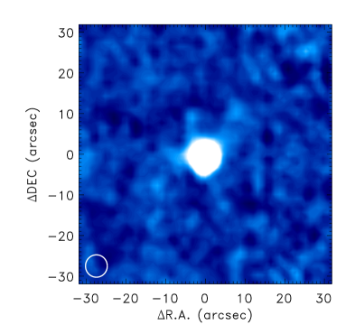
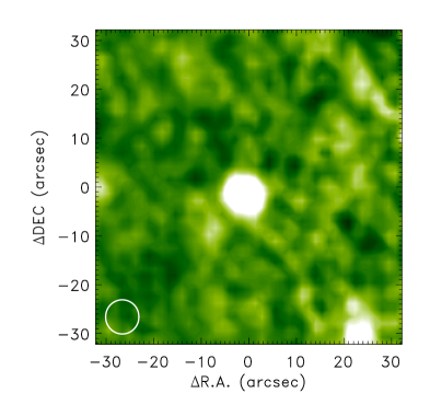
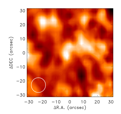
Double differential

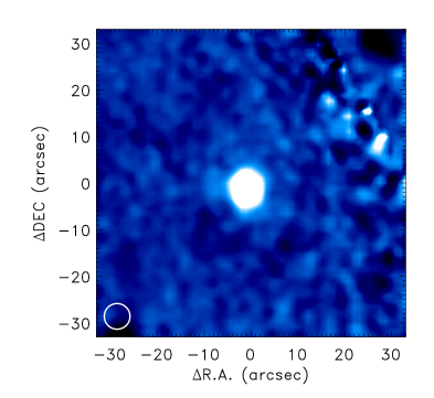
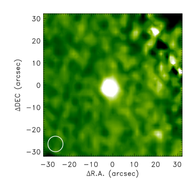
Figure 1: Image stamps showing the Herschel/PACS maps of 2013 AZ₆₀ in the $70\,\mu{\rm m}$ (blue), $100\,\mu{\rm m}$ (green), and $160\,\mu{\rm m}$ (red) channels. Each stamp covers an area of $64^{\prime\prime}\times 64^{\prime\prime}$, while the tick marks on the axes show the relative positions in pixels. The effective beam size (i.e. the circle with a diameter corresponding to the full width at half maximum) is also displayed in the lower-left corners of the stamps. The upper panels show the stamps directly combined from the individual frames where the lower stamps are obtained using the double-differential method. Due to the failure of the half of the red channel and the astrometric uncertainties, the second visit is nearly unusable in red, hence double-differential maps cannot be created.

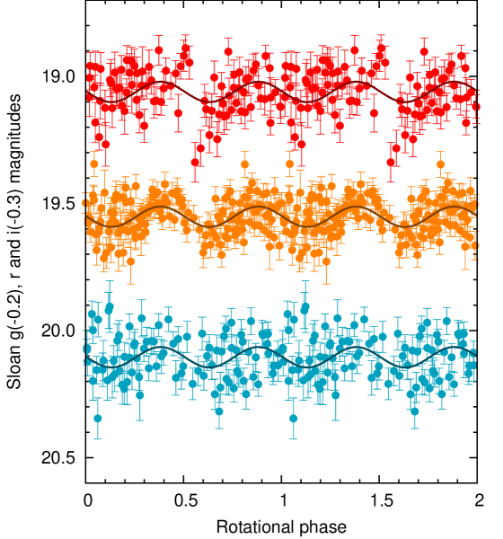
Figure 2: Folded optical light curves of 2013 AZ₆₀ using photometric data taken on 6 subsequent nights of 2013 November 4 – 9. Note that the folding frequency is related to the preferred double-peaked solution, $n=(5.11/2)\,{\rm d}^{-1}$. See text for further details.

Figure 3: Reflectance spectrum of 2013 AZ₆₀, taken with the OSIRIS spectrometer on the GTC in January, 2014. This spectrum is normalized to unity at $\lambda=5500\,{\rm\AA}$.

2.2 Optical photometry

Since 2013 AZ₆₀ has recently been discovered, one of our goals was to obtain precise photometric time series for this object in order to estimate both the absolute magnitudes (in various passbands) and the rotational period based on light curve variability. For these purposes, we used the IAC-80 telescope located at Teide Observatory, Tenerife. During our observing runs, we used the CAMELOT camera, equipped with a CCD-E2V detector of $2{\rm k}\times 2{\rm k}$, with a pixel scale of $\approx 0.3^{\prime\prime}$ providing a field of view of roughly $10^{\prime}\times 10^{\prime}$. Time series were gathered for several hours on the nights of 2013 November 4 – 9 using Sloan $g^{\prime}$, $r^{\prime}$ and $i^{\prime}$ filter sets. Since 2013 AZ₆₀ can currently be found at the edge of the spring Sloan field, several dozen stars with accurate reference magnitudes were available on each image. The night conditions were photometric on 5th, 7th and 9th of 2013 November where the individual photometric uncertainties were nearly constant and varied between $0.04$ and $0.05$ mags in Sloan $r^{\prime}$ band. The conditions were worse on the three another nights (4th, 6th and 8th) when the formal uncertainties scattered in the range of $0.04-0.08$ indicating the variable transparency of the sky (which was also notable during the observations). The worst conditions were on the first night where some of the measurements had a formal uncertainty of $0.09$.

The scientific images were analyzed with the standard calibration, source extraction, astrometry, cross matching and photometry tasks of the FITSH package (Pál, 2012). As a hint, we used the MPC predictions for the target coordinates and then we performed individual centroid fit on each image and smoothed with polynomial regression for a better (much more precise and accurate) input for aperture photometry. Instrumental magnitudes were then extracted for both the reference stars and the target itself and then after applying the standard photometric transformations, we obtained the intrinsic $g^{\prime}$, $r^{\prime}$ and $i^{\prime}$ magnitudes.

We searched for possible light curve variations using the most frequently sampled Sloan r’ band data (every second image was taken in Sloan $r^{\prime}$ while every fourth image was in $g^{\prime}$ and $i^{\prime}$). In order to search for periodic variations in our data set, we fitted a function in a form of $f(t)=a+b\cdot\sin(2\pi nt)+c\cdot\cos(2\pi nt)$ to the Sloan $r^{\prime}$ photometric series where $t$ indicates the independent value (the time in this case). If the value of $n$ is scanned in the appropriate domain ($n=0.01\dots 15$) with a proper stepsize ($n=0.01$, that is $\sim 8$ times smaller than the stepsize implied by the Nyquist criterion), then the parameters $a$, $b$ and $c$ can be obtained via a simple weighted linear least squares fit procedure. The unbiased $\chi^{2}$ values can then be compared with the reference value of $\chi^{2}_{0}$. This reference value is obtained when $n$ is set to $0$ and the error bars are scaled by a factor of $1.51$ to yield a $\chi^{2}_{0}$ equivalent to the degrees of freedom. The difference between the $\chi^{2}_{0}$ and the $\chi^{2}$ related to the adopted period tells the significance of the detection while various additional possible periods can also be checked and/or ruled out according to the difference between the respective $\chi^{2}$ values. We found a significant variation ($\chi^{2}_{0}-\chi^{2}=24.2$) with a corresponding amplitude of $\Delta{\rm r^{\prime}}=0.045\pm 0.007$ that has a frequency of $n=5.11\pm 0.12\,{\rm d}^{-1}$. The folded light curves are displayed in Fig. 2. The mean magnitudes of these observations were $g^{\prime}_{1}=20.274\pm 0.013$, $r^{\prime}_{1}=19.519\pm 0.009$ and $i^{\prime}_{1}=19.316\pm 0.013$.

We have to note here that due to the daily aliases, the peaks around $n\pm 1\,{\rm d}^{-1}$ are also remarkable and there is a non-negligible chance that one of these frequencies belong to the intrinsic rotation of the object. The peak at $n=6.11$ has a $\chi^{2}$ value which is only larger than that of the main peak by $3.5$.

In general, minor bodies in the Solar System feature double-peaked light curves. Hence, the rotational frequency of 2013 AZ₆₀ is more likely $n_{\rm rot}=n/2\,{\rm d}^{-1}$, equivalent to a period of $P_{\rm rot}=9.39\pm 0.22\,{\rm h}$. In order to test the significance of a double-peaked light curve solution, we coadded a sinusoidal component with half of the frequency to the primary variations. The amplitude of this component is found to be $0.013\pm 0.008\,{\rm mag}$. This is only a 1.7-$\sigma$ detection, however, a good argument for confirming the assumption for an intrinsic rotation period of $P_{\rm rot}\approx 9.4\,{\rm h}$.

In addition, we repeated the photometric observations for 2013 AZ₆₀ in 2014 January 28 in $g^{\prime}$ and $r^{\prime}$ bands. The results of these photometric measurements yielded the Sloan magnitudes of $g^{\prime}_{2}=19.71\pm 0.04$ and $r^{\prime}_{2}=18.99\pm 0.03$. During the first series of measurements (in 2013 November), the geocentric and heliocentric distance of 2013 AZ₆₀ were $\Delta_{1}=8.176\,{\rm AU}$ and $r_{1}=8.244\,{\rm AU}$, respectively, while in 2014 January 28, these distances were $\Delta_{2}=7.148\,{\rm AU}$ and $r_{2}=8.114\,{\rm AU}$. Based on these distances, the expected change in the apparent brightness was $5[\log_{10}(r_{2}\Delta_{2})-\log_{10}(r_{1}\Delta_{1})]=-0.326$, however, the actual brightness changes were $\Delta g^{\prime}=-0.56\pm 0.04$ and $\Delta r^{\prime}=-0.53\pm 0.03$, whose mean is $\Delta m=-0.54\pm 0.03$. Since the phase angle of 2013 AZ₆₀ was $\alpha_{1}=6.9^{\circ}$ in 2013 November 5 and $\alpha_{2}=1.5^{\circ}$ in 2014 January 28, these values imply a phase correction factor of $\beta=[(0.54\pm 0.03)-0.326]/(6.9-1.5)=0.039\pm 0.006\,{\rm mag}/{\rm deg}$. This is is rather good agreement with MPC observations. Based on the MPC observation database, the best-fit phase correction parameter can also be derived, however, with a larger uncertainty: $\beta_{\rm MPC}=0.040\pm 0.025\,{\rm mag}/{\rm deg}$.

These parameters allowed us to derive the absolute brightness of the object 2013 AZ₆₀ in a manner described in the following. First, we employed simple Monte-Carlo run whose input were the observed Sloan brightnesses, the derived phase correction factor as well as the parameters and the respective uncertainties of the corresponding Sloan-UBVRI transformation equation (for converting $g^{\prime}$ and $r^{\prime}$ brightnesses to $V$, see Jester et al., 2005). This Monte-Carlo run yielded a value of $H_{V}=10.42\pm 0.07$. Next, we checked the available photometric data series presented in the MPC database which yielded slightly fainter values, namely $H_{V,{\rm MPC}}=10.60\pm 0.15$. In order to reflect MPC photometry in our derived absolute brightness value, we adopted the weighted mean value of these two values, namely $H_{V}=10.45$ with a conservative uncertainty of $\pm 0.10$ in the subsequent modelling.

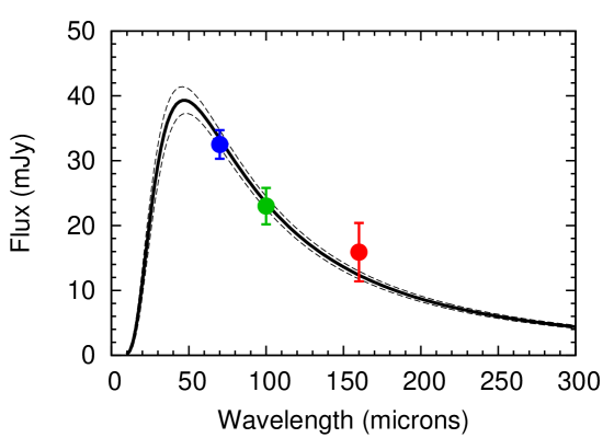
Figure 4: Spectral energy distribution of 2013 AZ₆₀ in the far-infrared region, based on Herschel/PACS measurements. Left panel: far-infrared measurements superimposed are the best-fit NEATM curves with their respective uncertainty. Middle panel: TPM model curve for thermal inertia of $100\,{\rm J}{\rm m}^{-2}{\rm K}^{-1}{\rm s}^{-1/2}$, rotation period of $9.39\,{\rm h}$ and equator-on geometry. Right panel: the value of $\chi^{2}$ as the function of thermal inertia for pole-on and equator-on geometries. See text for further details.

2.3 Reflectance spectrum

In order to accurately compare the surface colour characteristics of 2013 AZ₆₀ with other TNOs (see Lacerda et al., 2014), we obtained a low resolution spectrum using the Optical System for Imaging and Low Resolution Integrated Spectroscopy (OSIRIS) camera spectrograph (Cepa et al., 2000; Cepa, 2010) at the 10.4m Gran Telescopio Canarias (GTC), located at the El Roque de los Muchachos Observatory (ORM) in La Palma, Canary Islands, Spain. The OSIRIS instrument consists of a mosaic of two Marconi CCD detectors, each with $2048\times 4096$ pixels and a total unvignetted field of view of $7.8^{\prime}\times 7.8^{\prime}$, giving a plate scale of $0.127^{\prime\prime}/{\rm pixel}$. However, to increase the signal to noise for our observations we selected the $2\times 2$ binning mode with a readout speed of $200\,{\rm kHz}$ (that has a gain of $0.95\,{\rm e^{-}/ADU}$ and a readout noise of $4.5\,{\rm e^{-}}$), as corresponds with the standard operation mode of the instrument. A $300\,{\rm s}$ exposure time spectrum was obtained on January 28.17 (UTC), 2014 at an airmass of $X=1.14$ using the OSIRIS R300R grism that produces a dispersion of $7.74\,{\rm\AA/pixel}$, covering the $4800-9000\,{\rm\AA}$ spectral range. A $1.5^{\prime\prime}$ slit width was used oriented at the parallactic angle.

Spectroscopic reduction has been done using the standard IRAF tasks. Images were initially bias and flat-field corrected, using lamp flats from the GTC Instrument Calibration Module. The two-dimensional spectra were then wavelength calibrated using Xe+Ne+HgAr lamps. After the wavelength calibration, sky background was subtracted and a one dimensional spectrum was extracted. To correct for telluric absorption and to obtain the relative reflectance, G2V star Land102_1081 (Landolt, 1992) was observed using the same spectral configuration and at a similar airmass immediately after the Centaur observation. The spectrum of the 2013 AZ₆₀ was then divided by that of Land102_1081, and then normalized to unity at $0.55\,{\rm\mu m}$.

The derived spectrum is displayed in Fig. 3. Based on this spectrum, the slope parameter of this object is found to be $S^{\prime}=13.4\pm 3.0\,\%(1000\mathrm{\AA})^{-1}$ by a linear fit across the interval $5000-9000\,{\rm\AA}$.

The measured photometric colours ($g^{\prime}-r^{\prime}=0.755\pm 0.018$ and $0.72\pm 0.05$ on 2013.11.04 and 2014.01.28, respectively) are in complete accordance with the derived spectral slope. The spectrum was normalized at $5500\,{\rm\AA}$, just between the $g^{\prime}$ and $r^{\prime}$ bands. We can therefore write $S^{\prime}$ to equation (2) of Jewitt (2002), if we write SDSS colours instead of Bessel ones, and set $\Delta\lambda=1480\,{\rm\AA}$. This results in a synthetic colour index from spectral slope $(g-r)_{synth}=0.76\pm 0.04$, in a perfect agreement with our photometry within the errors.

2.4 Near-infrared photometry

CCD observations of 2013 AZ₆₀ were obtained on 24 September 2013 with the 4.2-m William Herschel Telescope at La Palma Observatory, equipped with the LIRIS instrument. LIRIS is a near-IR imager/spectrograph, which uses a $1{\rm k}\times 1{\rm k}$ HAWAII detector with a field of view of $4.27^{\prime}\times 4.27^{\prime}$. The number of exposures taken in different filters are: $5\times 30\,{\rm s}$ in $Y$ and $J$, $15\times 20\,{\rm s}$ in $H$, $15\times 13\,{\rm s}$ in CH4, and $180\times 20\,{\rm s}$ exposures in $K_{\rm s}$. Local comparison stars were selected from the 2MASS catalogue and magnitude transformation were applied following Hodgkin et al. (2009).

The result of the photometry is $Y=18.66\pm 0.08$, $J=18.34\pm 0.05$, $H=18.00\pm 0.06$ and $K_{\rm s}=17.72\pm 0.10$ where $Y$ refers to the UKIDDS system, while $JHK_{\rm s}$ are 2MASS magnitudes. Thus, 2013 AZ₆₀ exhibits almost exactly solar colour indices, with a slightly redder slope than solar. Namely $Y-J=0.32$, $J-H=0.34\pm 0.07$ and $H-K_{s}=0.28\pm 0.11$ while according to Casagrande et al. (2012) and estimating solar $Y-J$ according to Hodgkin et al. (2009), the respective solar colours are $(Y-J)_{\odot}=0.235\pm 0.018$ $(J-H)_{\odot}=0.286\pm 0.018$ and $(H-K_{s})_{\odot}=0.076\pm 0.018$. We note here that LIRIS is equipped with Mauna Kea Observatories (MKO) system of $J$, $H$ and $K$ filters. According to Hodgkin et al. (2009), the expected systematic differences between 2MASS and LIRIS/MKO colours of 2013 AZ₆₀ is in the range of $-0.010\dots+0.015$, which is definitely smaller than the photometric uncertainties. This observation indicates a flat and featureless spectrum of 2013 AZ₆₀: the slope is equivalent in the infrared and in the optical, being quite similar to dormant cometary nuclei.

During the observation the heliocentric and geocentric distance of 2013 AZ₆₀ were $8.87$ and $8.32\,{\rm AU}$, respectively, indicating an absolute mid-IR brightness of $J=9.00\pm 0.06$ without correcting for the solar phase angle.

Table 3: Orbital and optical data for 2013 AZ₆₀ at the time of the Herschel observations.

Quantity	Symbol	Value
Heliocentric distance	$r$	$8.702$ AU
Distance from Herschel	$\Delta$	$8.560$ AU
Phase angle	$\alpha$	$6.\!\!^{\circ}6$
Absolute visual magnitude	$H_{V}$	$10.45\pm 0.10$

3 Thermal emission modelling

3.1 Near-Earth Asteroid Thermal Model

The basic physical properties such as albedo and diameter can be obtained by combining optical brightness data with thermal emission. Assuming an absolute optical brightness for a certain object, the higher the thermal emission, the smaller the actual albedo and hence the larger the diameter. Due to the observing strategies constrained by the spatial attitude of the Herschel, objects close to the ecliptic are likely observable by Herschel during quadratures. Nevertheless, in quadratures these minor objects exhibit a large phase angle, hence Standard Thermal Model (STM Lebofsky et al., 1986) might not be as accurate as it is desired. 2013 AZ₆₀ had a phase angle of $\alpha=6.6^{\circ}$ at the time of our Herschel/PACS observations. In order to have accurate estimates for larger phase angles, we employed the Near-Earth Asteroid Thermal Model (NEATM Harris, 1998): this model integrates the thermal emission for arbitrary viewing angles. Throughout the modelling we use the heliocentric and geocentric distances at the instance of the Herschel/PACS measurements, namely $r_{\rm helio}=8.702\,{\rm AU}$ and $r_{\rm geo}=8.560\,{\rm AU}$.

The diameter and albedo can then be derived in a similar manner like in our earlier works (see e.g. Kiss et al., 2013; Pál et al., 2012). As an input for the fit procedures, we used the previously obtained thermal fluxes (see Table 2) and the absolute brightness $H_{V}=10.45\pm 0.10$ (derived earlier, see above).

The absolute physical parameters (diameter, albedo and beaming parameter) have been obtained in a Monte-Carlo fashion. In each step, a Gaussian value were drawn for the four input values (three thermal fluxes and the absolute brightness $H_{V}$) and the model parameters were adjusted via a nonlinear Levenberg-Marquardt fit. A sufficiently long series of such steps yields the best fit values as well as the respective uncertainties and correlations. This procedure were performed in two iterations. First, we let the value for the beaming parameter $\eta$ to be floated. This run resulted relatively high correlations between the parameters and a highly long-tailed distribution for $\eta$: we found that the mode for $\eta$ was $0.8$ while the median is $2.6$ and the uncertainties yielded by the lower and upper quartiles are $2.6^{+2.9}_{-1.1}$. This skewed distribution is due to the fact that beaming parameters cannot really be constrained if thermal fluxes are not known for shorter wavelengths (i.e. shorter than the peak of the spectral energy distribution). Hence, in the next run we used $\eta$ as an input (instead of an adjusted variable) while its value was drawn uniformly between $0.8$ and $2.6$. This domain is also in accordance with the possible physical domain of the beaming parameter (see also Fig. 4 of Lellouch et al., 2013). The results of this second run were $d=62.3\pm 5.3\,{\rm km}$, $p_{V}=0.029\pm 0.006$ while the beaming parameter can be written as $\eta=1.7\pm 0.9$. The resulting albedo refers to a remarkably dark surface. The fluxes along with the best-fit NEATM model curve are shown in the left panel of Fig. 4.

3.2 Thermophysical Model

In addition to the derivation of the NEATM parameters, we conducted an analysis of thermal emission based on the asteroid thermophysical model (TPM, see Müller & Lagerros, 1998, 2002). The observational constraints employed by this model was the thermal fluxes (see Table. 2), the absolute magnitude of $H_{V}=10.45\pm 0.10$ (see earlier), the rotational period of $9.39\,{\rm h}$ as well as the actual geometry at the time of Herschel observations (see the values for phase angle, heliocentric and geocentric distances above).

Our procedures have shown that the best-fit model occurs at high thermal inertia values. Assuming an equator-on geometry, a value for reduced $\chi^{2}\lesssim 1$ corresponds to $\Gamma\gtrsim 10\,{\rm J}{\rm m}^{-2}{\rm K}^{-1}{\rm s}^{-1/2}$ (see also the right panel of Fig. 4), however, the gradually decreasing form of the function $\chi^{2}(\Gamma)$ implies a lower limit of $\Gamma\gtrsim 50\,{\rm J}{\rm m}^{-2}{\rm K}^{-1}{\rm s}^{-1/2}$. The corresponding values at $\Gamma=50\,{\rm J}{\rm m}^{-2}{\rm K}^{-1}{\rm s}^{-1/2}$ for geometric albedo and diameter are $p_{V}=0.028$ and $d=64.9\,{\rm km}$, respectively. These values are also compatible within uncertainties with the ones derived from NEATM analysis (see above). The spectral energy distribution provided by these TPM values are shown in the middle panel of Fig. 4. This value for the thermal inertia is close to the values of $30-300\,{\rm J}{\rm m}^{-2}{\rm K}^{-1}{\rm s}^{-1/2}$ reported for comets (Julian, Samarasinha & Belton, 2000; Campins & Fernández, 2000; Davidsson et al., 2013, see e.g.) as well as the value of $10-50\,{\rm J}{\rm m}^{-2}{\rm K}^{-1}{\rm s}^{-1/2}$ for 67P/Churyumov-Gerasimenko (Gulkis et al., 2015). We note here that models either with thermal inertia values smaller than $50\,{\rm J}{\rm m}^{-2}{\rm K}^{-1}{\rm s}^{-1/2}$ or having an assumption for pole-on view underestimate the observed flux at $160\,{\rm\mu m}$.

Our findings for large preferred values of the beaming parameter $\eta$ as well as for the thermal inertia $\Gamma$ (even $\Gamma\gtrsim 10\,{\rm J}{\rm m}^{-2}{\rm K}^{-1}{\rm s}^{-1/2}$) can be compared with the statistical expectations of Lellouch et al. (2013). By considering the small heliocentric distance of this object, both of these values are expected to be smaller (see Figs. 6 and 11 in Lellouch et al., 2013).

4 The dynamics of 2013 AZ₆₀

2013 AZ₆₀ moves on a highly eccentric orbit, with perihelion between the orbits of Jupiter and Saturn. The best fit solution for the epoch of March 15, 2015 is shown in Table 4.

Table 4: The best-fit orbital solution (semi-major axis $a$, perihelion distance $q$, eccentricity $e$, inclination $i$, longitude of ascending node $\Omega$, argument of perihelion $\omega$, mean anomaly $M$ and perihelion date $T_{\rm peri}$), and associated uncertainties, for 2013 AZ₆₀, taken from the Minor Planet Center (http://www.minorplanetcenter.net) on March 15, 2015. Note that the uncertainties of the orbital elements involved throughout the planning of the observations significantly larger than these due to the shorter arcs available at that time.

a (AU)	829.7
q (AU)	7.908098 $\pm$ 0.000014
e	0.990468 $\pm$ 0.000010
i (deg)	16.535760 $\pm$ 0.000011
$\Omega$ (deg)	349.21122 $\pm$ 0.00002
$\omega$ (deg)	158.14327 $\pm$ 0.00021
M (deg)	0.00876
$T_{\rm peri}$	2456988.0641 $\pm$ 0.0032
Epoch (JD)	2457200.5

In order to assess the dynamical history, and potential future behaviour of 2013 AZ₆₀, we follow a well-established route (see e.g. Horner et al., 2004a, b, 2010, 2012; Kiss et al., 2013), and used the Hybrid integrator within the n-body dynamics package MERCURY (Chambers, 1999), to follow the evolution of a swarm of test particles centered on the best-fit orbit for the object, in order to get a statistical overview of the object’s behaviour. A total of 91,125 test particles were created, distributed uniformly across the region of orbital element phase space within $\pm 3\sigma$of the best-fit perihelion distance, $q$, eccentricity, $e$, and inclination, $i$. In this manner, we created a grid of $45\times 45\times 45$ test particles distributed in even steps across the $\pm 3\sigma$ error ranges about the nominal best fit orbit in each of the three orbital elements studied. Each of these test particles was then followed in our integrations, with its orbit evolving under the gravitational influence of the giant planets Jupiter, Saturn, Uranus and Neptune, for a period of four billion years. Test particles were considered to have been ejected from the Solar System (and were therefore removed from the integrations) if they reached a barycentric distance of 10,000 AU. Similarly, any test particles that collided with one of the giant planets, or with the Sun, were removed from the simulations. Each time a test particle was removed in either of these manners, the time at which the removal occurred was recorded, allowing us to track the number of surviving test particles as a function of time. The results of our simulations are shown below, in Figs 5 and 6.

Figure 5: The decay of our population of 91,125 clones of 2013 AZ₆₀ as a function of the time elapsed in our integrations. The plots on the right show the same data as those on the left, but are plotted on a log/log scale. The upper panels show the decay of the population over the first billion years of the four billion year integrations, whilst the lower panels show the decay over the first million years.

It is immediately apparent that the population of clones of 2013 AZ₆₀ is highly dynamically unstable, with 63.9% of the particles (58191 of 91125) being removed from the simulations within the first million years of the integrations, as a result of either ejection or collision with one of the giant planets or the Sun. Half of the test particles are ejected within the first 682 kyr of the integrations, revealing that the orbit of 2013 AZ₆₀ is more than two orders of magnitude more unstable than that of the similar object 2012 DR₃₀ (Kiss et al., 2013).

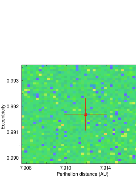
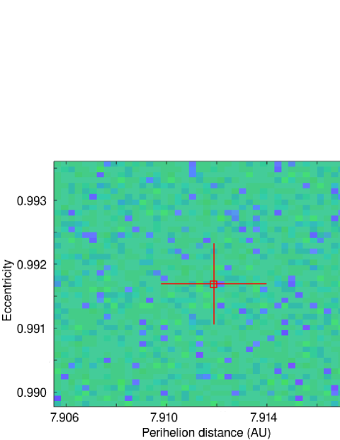
Figure 6: The mean (upper) and median (lower) lifetimes of 2013 AZ₆₀, as a function of the initial perihelion distance, q, and eccentricity, e, of the orbit tested. The location of the best-fit orbital solution for 2013 AZ₆₀, as detailed in Table 4, is shown by the hollow square at the center of the figure, with the $\pm$1$\sigma$ uncertainties on the perihelion distance and eccentricity denoted by the solid black lines that radiate from that box. Each coloured square in the figures shows the mean (or median) lifetime of the 45 individual runs carried out at that particular a-e location. Each of those 45 runs tested a different orbital inclination for 2013 AZ₆₀, evenly distributed across the $\pm 3\sigma$ uncertainty range on the best-fit orbital solution. As was the case with the high-eccentricity Centaur 2012 DR₃₀ (Kiss et al., 2013), the stability of the orbit of 2013 AZ₆₀ does not vary significantly across the range of perihelion distance and eccentricities tested in this work – a reflection of the relatively high precision with which the object’s orbit is known.

The orbit of 2013 AZ₆₀ proves to be highly dynamically unstable on timescales of just a few hundred thousand years. Fully half of the test particles in our simulations were removed from the simulations within just 682 kyr, and almost two-thirds were removed within the first million years. This extreme level of instability is not, however, that surprising – 2013 AZ₆₀ passes through the descending node of its orbit at essentially the same time it passes through perihelion, maximizing the likelihood that it will be perturbed by either Jupiter or Saturn. This extreme level of instability is typical of objects moving on Centaur like orbits (e.g. Horner et al., 2004a, b) and suggests that 2013 AZ₆₀ may only recently have been captured to its current orbit. This argument is supported by the fact that, averaged over our entire population of 91,125 test particles, the mean lifetime of 2013 AZ₆₀ is just 1.56 Myr.

Given that 2013 AZ₆₀ exhibits such extreme instability, and may well be relatively pristine object, it is interesting to consider whether it will have experienced significant solar heating, and cometary activity, over its past history. As a result of our large dynamical dataset on the evolution of 2013 AZ₆₀, it is possible to determine the fraction of the population of clones that may one day evolve onto Earth-crossing orbits, and the fraction of the population that approach the Sun to within a given heliocentric distance at some point in their lifetime. Since dynamical evolution under the influence of gravity alone is a time-reversible process, we can use these values to estimate the probability that 2013 AZ₆₀ has moved on orbits that bring it within those heliocentric distances at some point in the past, before being ejected to its current orbit. Due to the extreme instability exhibited by 2013 AZ₆₀, we found that a relatively small number of the total population of clones were captured to Earth-crossing orbits through their lifetimes. Indeed, just 3805 of the 91125 test particles we studied (just 4.2% of the population) became Earth-crossing at any point in our integrations, and the total fraction of the object’s lifetime spent as an Earth-crossing object (averaged across all 91125 test particles) was 0.12%. Our results for a variety of other perihelion distances are displayed in Table 5, together with estimates of the mean amount of time for which clones of 2013 AZ₆₀ exhibited perihelion distances smaller than the specified value.

	Number of clones	Percentage of total
		integration time
Earth-crossing	3805	0.118
($q<1.0616\,{\rm AU}$)
$q<2\,{\rm AU}$	6005	0.291
$q<4\,{\rm AU}$	12272	0.329
$q<6\,{\rm AU}$	27150	2.06

Table 5: The number of the 91,125 clones of 2013 AZ₆₀ simulated in this work that evolved to orbits with perihelion distances smaller than 2, 4, and 6 AU, and the number that evolved onto Earth-crossing orbits (following Horner et al., 2003). For each of these values, we also give the fraction of the total integration time, across all 91,125 clones, for which clones have perihelion distances within these limits. We note that this is the fraction of the time for which the perihelion distance was less than the stated amount and not the fraction of time the clones spend within that heliocentric distance. Even when moving on an orbit with perihelion within that of the Earth, a given clone will spend the vast majority of its time beyond that distance, and only a tiny fraction within it.

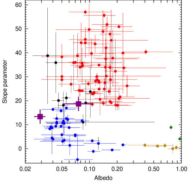
Figure 7: Slope parameter vs. albedo relations for 111 TNOs, including 2013 AZ₆₀ and 2012 DR₃₀. Data (except for these two latter objects) have been taken from Lacerda et al. (2014). The blue and red dots indicate the two major groups identified by Lacerda et al. (2014), black points represent ambiguous objects (due to their large respective uncertainties) while green and yellow dots show the large bodies and Haumea-type surfaces, respectively. The isolated purple square shows the place of 2013 AZ₆₀ at the very left side of the diagram. The other purple square indicates 2012 DR₃₀, just in between of the dark neutral (blue) and bright red (red) object groups.

5 Discussion

Since the orbit of 2013 AZ₆₀ is highly eccentric, and takes the object out to approximately $1950\,{\rm AU}$, it is clear that it spends the vast majority of its orbit at large heliocentric distance. It is quite plausible that 2013 AZ₆₀ is a relatively recent entrant to the inner Solar System. Hence, it is interesting to consider how much time, cumulative over its entire history since it was first emplaced on a planet crossing orbit, has it spent at a heliocentric distance of less than 1, 10 or 100 AU. Again, we can take advantage of the large dynamical dataset available to us from our integrations to get a feel for the amount of time the object will have spent within these distances. Clearly, this is only an estimate (and implicitly assumes that, prior to its injection to a planet-crossing orbit, the object was well beyond the 100 AU boundary – i.e. that it was injected from the inner or outer Oort cloud, rather than the trans-Neptunian region). Given that implicit assumption, we find that, on average, clones of 2013 AZ₆₀ spend just 6.68 years within 1 AU of the Sun, 4620 years within 10 AU of the Sun, and 273,000 years within 100 AU of the Sun. The time spent within 10 and 100 AU is strongly biased by a few particularly long-lived clones, especially those that are captured onto Centaur-like orbits. We note that more than two-thirds of the clones (64904 objects) spent less than a thousand years within 100 AU of the Sun, and 37493 (41.1%) spent less than one hundred years within 100 AU. Taken into considerations, our dynamical results suggest that 2013 AZ₆₀ has only recently been captured to its current planet-crossing orbit, and that it is quite likely that it is a relatively pristine object. Indeed, it seems highly probable that the surface of 2013 AZ₆₀ has experienced only minimal outgassing and loss of volatiles since being captured to a planet crossing orbit, and so it represents a particularly interesting object to target with further observations as it pulls away from the Sun following its recent perihelion passage.

Outer Solar System objects can also be characterized in a way recently put forward by Lacerda et al. (2014), using their visual range colours and albedos. In this frame, Centaurs and trans-Neptunian objects form typically two clusters, a dark-neutral and a bright-red one (see Fig. 2 in Lacerda et al., 2014). In this scheme, 2013 AZ₆₀ is located at the dark (very low albedo) edge of the dark-neutral cluster, see Fig. 7. 2013 AZ₆₀ is even darker than the object 2002 GZ₃₂, the object with the lowest albedo in the sample of Duffard et al. (2014). Objects with characteristics similar to our target belong rather to “dead comets” or Jupiter family comets which are the end states of Centaurs and Oort cloud comets (Fig. 4 in Lacerda et al., 2014); in this sense 2013 AZ₆₀ is more similar to objects in the inner Solar System than those in the trans-Neptunian population. We also checked the distribution of the slope parameters of various Centaurs based on Fornasier et al. (2009). Although in that work, a correlation between the slope parameters and orbital eccentricity were suspected (the higher the eccentricity, the redder the object), the large eccentricity of 2013 AZ₆₀ do not fit in this model since it has definitely lower slope parameter than the mean of that sample of Centaurs.

While the dynamical analysis indicate that 2013 AZ₆₀ has recently been pulled from the Oort cloud, in the case of this object there is a much higher likelihood that it has spent a considerable time in the inner Solar System then e.g. in the case of 2012 DR₃₀, which might just be in a transitional phase between the two main albedo-colour clusters (Kiss et al., 2013).