Isotropic and anisotropic pointing models

Abstract

This paper describes an alternative approach for generating pointing models for telescopes equipped with serial kinematics, esp. equatorial or alt-az mounts. Our model construction does not exploit any assumption for the underlying physical constraints of the mount, however, one can assign various effects to the respective components of the equations. In order to recover the pointing model parameters, classical linear least squares fitting procedures can be applied. This parameterization also lacks any kind of parametric singularity. We demonstrate the efficiency of this type of model on real measurements with meter-class telescopes where the results provide a root mean square accuracy of $1.5-2$ arcseconds.

1 Introduction

Pointing models are widely exploited in telescope control in order to correct for mechanical and manufacturing imperfections of the various parts of the system. The basic concept of a pointing model is to figure out and quantify the difference between the targeted and the apparent position of the telescope throughout the observations. This quantification can be done using lookup tables with some grid spacing as well as using analytical approaches where these functions are related to the physical behaviour of the telescope mechanics.

In most of the pointing models, either in the case of equatorial mounts (Spillar et al., 1993), altitude-azimuth mounts (Granzer et al., 2012; Zhang & Wu, 2001) or complex systems of more telescopes (Gothe et al., 2013) the raw, uncorrected positions of the various axes (hour axis, declination axis, azimuth axis or elevation axis) are read from high precision rotary encoders. Such encoders provide a precision within fractions of arcseconds or even hundredths of arcseconds. There are other types of pointing models that involve MEMS accelerometers (Mészáros et al., 2014) instead of such encoders. The attainable precision is much lower in the case of these integrated accelerometers (currently it is in the range of an arcminute). Despite the lower precision, these solutions also have advantages, including the redundant operation (via the various constraints between the accelerometer channels), the resistance to unintentional tampering and the possibility of installation without modifying or altering the drivers.

The goal of our work presented here is to provide a strictly mathematical approach for finding analytical pointing models which provide an RMS accuracy within a few arcseconds. First, in Sec. 2 we detail the mathematical formalism used in the derivation of an isotropic pointing model. This model is then extended in Sec. 3 with terms that quantify a generalized form of dependence by performing expansions of spherical harmonics. These expansions allow the model to take into account various forms of anisotropic behaviour, for instance the torques inducted by gravity or misalignments of the gearing. In Sec. 5 we report results of test measurements validating these models, as well as we detail how the pointing model can be implemented. Finally, our work is summarized in Sec. 6.

2 Isotropic pointing model

Basically, telescope mechanics are treated as a serial robot formed by two subsequent stages where the two stages are performing (nearly) orthogonal rotation. Throughout this paper we present the calculations in first equatorial coordinate system, however, a similar approach can be involved for alt-az mechanics by simply replacing the variables appropriately. In the case of an equatorial mount, the first shaft (whose bearings are fixed to the ground) is responsible for the rotation around the hour axis while the second, perpendicular stage is responsible for setting the declination. In the following, we recall briefly the main ideas behind the isotropic approach used in Mészáros et al. (2014).

Throughout the derivation of our models, let us exploit the Cartesian representation of celestial coordinates. Let us define the standard direction of the telescope tube to the $x+$ axis, i.e. without any rotation, the telescope directed to the vector of $\mathbf{p}_{0}=(1,0,0)$. This is in accordance with the historic parameterization of the first equatorial system if we treat the hour angle $\tau$ and declination $\delta$ values as polar angles. However, one should keep in mind that this parameterization yields a left-handed $(x,y,z)$ system of reference (see Fig. 1). An arbitrary point at the sky is then defined by the vector

$$\mathbf{p}=\begin{pmatrix}\cos\delta\cos\tau\\ \cos\delta\sin\tau\\ \sin\delta\end{pmatrix}$$ (1)

while $\mathbf{p}(\tau=0,\delta=0)\equiv\mathbf{p}_{0}$. If one treats the whole telescope system as a series of active rotations, then one can write

$$\mathbf{p}(\tau,\delta)=\mathbf{P}_{\rm t}\cdot\mathbf{P}_{\rm d}\cdot\mathbf{p}_{0}$$ (2)

where the rotation matrices $\mathbf{P}_{\rm t}$ and $\mathbf{P}_{\rm d}$ are defined as

$$\mathbf{P}_{\rm t} = \begin{pmatrix}\cos\tau&-\sin\tau&0\\ \sin\tau&\cos\tau&0\\ 0&0&1\end{pmatrix},$$ (3)

$$\mathbf{P}_{\rm d} = \begin{pmatrix}\cos\delta&0&-\sin\delta\\ 0&1&0\\ \sin\delta&0&\cos\delta\end{pmatrix}.$$ (4)

As it can be recognized, the assumption in Eq. (2) is valid only in ideal circumstances. In real applications, the various deflections presented in the telescope system are quantified by the rotation matrices $\mathbf{H}$, $\mathbf{X}$ and $\mathbf{T}$ using the relation

$$\mathbf{p}^{\prime}(\tau,\delta)=\big{(}\mathbf{H}\cdot\mathbf{P}_{\rm t}\cdot\mathbf{X}\cdot\mathbf{P}_{\rm d}\cdot\mathbf{T}\big{)}\cdot\mathbf{p}_{0}$$ (5)

Here, $\mathbf{H}$ quantifies the misalignments of the telescope hour axis with respect to the ground, $\mathbf{X}$ quantifies the misalignments of the declination axis with respect to the hour axis while $\mathbf{T}$ quantifies the misalignments of the detector or the tube with respect to the declination axis. These matrices of $\mathbf{H}$, $\mathbf{X}$ and $\mathbf{T}$ are quite close to unity. Hence, a first-order series expansion can be involved in order to approximate these. The idea is based on the well-known relation between skew-symmetric and orthogonal matrices. Namely, for any skew-symmetric matrix $\mathbf{A}=-\mathbf{A}^{\rm T}$, the exponential of $\exp(\mathbf{A})$ is always an orthogonal matrix with unity determinant. In practice, let us write these in the form of

$$\mathbf{H} = \exp\begin{pmatrix}0&-c&b\\ c&0&-a\\ -b&a&0\end{pmatrix}\approx\begin{pmatrix}1&-c&b\\ c&1&-a\\ -b&a&1\end{pmatrix}$$ (6)

$$\mathbf{X} = \exp\begin{pmatrix}0&-f&e\\ f&0&-d\\ -e&d&0\end{pmatrix}\approx\begin{pmatrix}1&-f&e\\ f&1&-d\\ -e&d&1\end{pmatrix}$$ (7)

$$\mathbf{T} = \exp\begin{pmatrix}0&-i&h\\ i&0&-g\\ -h&g&0\end{pmatrix}\approx\begin{pmatrix}1&-i&h\\ i&1&-g\\ -h&g&1\end{pmatrix}$$ (8)

We call the pointing model isotropic if the matrices $\mathbf{H}$, $\mathbf{X}$ and $\mathbf{T}$ do not depend on the telescope position.

Figure 1: The left-handed coordinate system implied by the first equatorial coordinates, i.e. the hour angle $\tau$ and the declination $\delta$.

Here we give the full expansion of $\mathbf{P}$ up to the first order. In the formula presented below, $c_{\rm t}$, $s_{\rm t}$, $c_{\rm d}$ and $s_{\rm d}$ denote $\cos\tau$, $\sin\tau$, $\cos\delta$ and $\sin\delta$, respectively:

$$\mathbf{P} \approx \begin{pmatrix}c_{\rm t}c_{\rm d}&-s_{\rm t}&-c_{\rm t}s_{\rm d}\\ s_{\rm t}c_{\rm d}&c_{\rm t}&-s_{\rm t}s_{\rm d}\\ s_{\rm d}&0&c_{\rm d}\end{pmatrix}+a\begin{pmatrix}0&0&0\\ -s_{\rm d}&0&-c_{\rm d}\\ s_{\rm t}c_{\rm d}&c_{\rm t}&-s_{\rm t}s_{\rm d}\end{pmatrix}$$ (9)

$$+ b\begin{pmatrix}s_{\rm d}&0&c_{\rm d}\\ 0&0&0\\ -c_{\rm t}c_{\rm d}&s_{\rm t}&c_{\rm t}s_{\rm d}\end{pmatrix}+c^{\prime}\begin{pmatrix}-s_{\rm t}c_{\rm d}&-c_{\rm t}&s_{\rm t}s_{\rm d}\\ c_{\rm t}c_{\rm d}&-s_{\rm t}&-c_{\rm t}s_{\rm d}\\ 0&0&0\end{pmatrix}$$

$$+ d\begin{pmatrix}s_{\rm t}s_{\rm d}&0&s_{\rm t}c_{\rm d}\\ -c_{\rm t}s_{\rm d}&0&-c_{\rm t}c_{\rm d}\\ 0&1&0\end{pmatrix}+e^{\prime}\begin{pmatrix}c_{\rm t}s_{\rm d}&0&c_{\rm t}c_{\rm d}\\ s_{\rm t}s_{\rm d}&0&s_{\rm t}c_{\rm d}\\ -c_{\rm d}&0&s_{\rm d}\end{pmatrix}$$

$$+ g\begin{pmatrix}0&-c_{\rm t}s_{\rm d}&s_{\rm t}\\ 0&-s_{\rm t}s_{\rm d}&-c_{\rm t}\\ 0&c_{\rm d}&0\end{pmatrix}+i\begin{pmatrix}-s_{\rm t}&-c_{\rm t}c_{\rm d}&0\\ c_{\rm t}&-s_{\rm t}c_{\rm d}&0\\ 0&-s_{\rm d}&0\end{pmatrix}.$$

During the expansion, the matrices proportional to $c$ and $f$ are going to be exactly the same like the matrices proportional to $e$ and $h$. Hence, the above equation depends only on $c+f$ and $e+h$. Therefore, in the following we use $c^{\prime}=c+f$ and $e^{\prime}=e+h$ in our computations.

If the expansion above (Eq. 9) is multiplied by the reference vector $\mathbf{p}_{0}$, the term proportional to $g$ will also vanish. This term effects computations only when the information provided by the apparent field rotation is also included in the pointing model since the first column of the respective matrix is identical to zero. All in all, the expansion of Eq. (5) is

$$\mathbf{p}^{\prime}(\tau,\delta) = \begin{pmatrix}c_{\rm t}c_{\rm d}\\ s_{\rm t}c_{\rm d}\\ s_{\rm d}\end{pmatrix}+a\begin{pmatrix}0\\ -s_{\rm d}\\ c_{\rm d}s_{\rm t}\end{pmatrix}+b\begin{pmatrix}s_{\rm d}\\ 0\\ -c_{\rm d}c_{\rm t}\end{pmatrix}$$ (10)

$$+ c^{\prime}\begin{pmatrix}-c_{\rm d}s_{\rm t}\\ c_{\rm d}c_{\rm t}\\ 0\end{pmatrix}+d\begin{pmatrix}s_{\rm d}s_{\rm t}\\ -s_{\rm d}c_{\rm t}\\ 0\end{pmatrix}$$

$$+ e^{\prime}\begin{pmatrix}s_{\rm d}c_{\rm t}\\ s_{\rm d}s_{\rm t}\\ -c_{\rm d}\end{pmatrix}+i\begin{pmatrix}-s_{\rm t}\\ c_{\rm t}\\ 0\end{pmatrix}.$$

This equation can be written in the form of

$$\mathbf{p}^{\prime}(\tau,\delta)=\mathbf{p}(\tau,\delta)+\sum\limits_{k=1}^{6}a_{k}\mathbf{p}_{k}(\tau,\delta),$$ (11)

where the vector $\mathbf{p}(\tau,\delta)$ is defined by Eq. (1), the parameter vector of $\mathbf{a}=(a_{1},\dots,a_{6})$ is equivalent to $(a,b,c^{\prime},d,e^{\prime},i)$ and the $\mathbf{p}_{k}(\tau,\delta)$ are defined accordingly to Eq. (10).

The parameters ($a_{k}$) can be obtained by a linear least squares regression if a series of observations is known with reported mount axis encoder positions of $(\tau_{n},\delta_{n})$ as well as the respective apparent positions of $(T_{n},D_{n})$. Here, “apparent” refers to the hour angle and declination values after correcting for precession, nutation, aberration and refraction as well as one should accurately obtain the ${\rm DUT1}={\rm UT1}-{\rm UTC}$ differences throughout the derivation of the local sidereal time instances (see Wallace, 2002, 2008, for more details). Once this series of $1\leq n\leq N$ measurements is known, one has to minimize the merit function

$$\chi^{2}=\sum\limits_{n=1}^{N}\chi^{2}_{n}$$ (12)

where

$$\chi^{2}_{n}=\left[\mathbf{p}(\tau_{n},\delta_{n})+\sum\limits_{k=1}^{6}a_{k}\mathbf{p}_{k}(\tau_{n},\delta_{n})-\mathbf{p}(T_{n},D_{n})\right]^{2}.$$

Minimization of the above equation for $\chi^{2}$ yields a linear array of equations whose solution is then straightforward. Due to the three dimensional nature of the $\mathbf{p}$ vectors, this equation for $\chi^{2}$ implies $3N$ independent terms. However, the effective number for degrees of freedom is only $2N-6$ since for all $1\leq k\leq 6$ values and for all observations,

$$\mathbf{p}(\tau_{n},\delta_{n})\cdot\mathbf{p}_{k}(\tau_{n},\delta_{n})=0.$$ (13)

In other words, these 6 base vectors of $\mathbf{p}_{k}$ defined in the expansion (11) are always perpendicular to the observation direction $\mathbf{p}(\tau_{n},\delta_{n})$.

In the following we extend the isotropic model described above with terms that provide significantly better accuracy.

Table 1: Coefficients of the expansion of the pointing model up to the first order in the spherical harmonics. Note that the terms marked with stars ($\bigstar$) and dots ($\bullet$) are not linearly independent. Hence, the first order expansion of the pointing model has 22 independent coefficients instead of 24.

	$Y_{00}$	$Y_{1,-1}$	$Y_{1,0}$	$Y_{0,1}$
$a$	$\begin{pmatrix}0\\ -s_{\rm d}\\ c_{\rm d}s_{\rm t}\end{pmatrix}$	$\begin{pmatrix}0\\ -s_{\rm d}c_{\rm d}s_{\rm t}\\ c_{\rm d}^{2}s_{\rm t}^{2}\end{pmatrix}$	$\begin{pmatrix}0\\ -s_{\rm d}^{2}\\ s_{\rm d}c_{\rm d}s_{\rm t}\end{pmatrix}$	$\begin{pmatrix}0\\ -s_{\rm d}c_{\rm d}c_{\rm t}\\ c_{\rm d}^{2}s_{\rm t}c_{\rm t}\end{pmatrix}_{\bullet}$
$b$	$\begin{pmatrix}s_{\rm d}\\ 0\\ -c_{\rm d}c_{\rm t}\end{pmatrix}$	$\begin{pmatrix}s_{\rm d}c_{\rm d}s_{\rm t}\\ 0\\ -c_{\rm d}^{2}s_{\rm t}c_{\rm t}\end{pmatrix}_{\bullet}$	$\begin{pmatrix}s_{\rm d}^{2}\\ 0\\ -s_{\rm d}c_{\rm d}c_{\rm t}\end{pmatrix}$	$\begin{pmatrix}s_{\rm d}c_{\rm d}c_{\rm t}\\ 0\\ -c_{\rm d}^{2}c_{\rm t}^{2}\end{pmatrix}$
$c^{\prime}$	$\begin{pmatrix}-c_{\rm d}s_{\rm t}\\ c_{\rm d}c_{\rm t}\\ 0\end{pmatrix}$	$\begin{pmatrix}-c_{\rm d}^{2}s_{\rm t}^{2}\\ c_{\rm d}^{2}s_{\rm t}c_{\rm t}\\ 0\end{pmatrix}$	$\begin{pmatrix}-s_{\rm d}c_{\rm d}s_{\rm t}\\ s_{\rm d}c_{\rm d}c_{\rm t}\\ 0\end{pmatrix}_{\bullet}$	$\begin{pmatrix}-c_{\rm d}^{2}s_{\rm t}c_{\rm t}\\ c_{\rm d}^{2}c_{\rm t}^{2}\\ 0\end{pmatrix}$
$d$	$\begin{pmatrix}s_{\rm d}s_{\rm t}\\ -s_{\rm d}c_{\rm t}\\ 0\end{pmatrix}_{\bigstar}$	$\begin{pmatrix}s_{\rm d}c_{\rm d}s_{\rm t}^{2}\\ -s_{\rm d}c_{\rm d}s_{\rm t}c_{\rm t}\\ 0\end{pmatrix}$	$\begin{pmatrix}s_{\rm d}^{2}s_{\rm t}\\ -s_{\rm d}^{2}c_{\rm t}\\ 0\end{pmatrix}$	$\begin{pmatrix}s_{\rm d}c_{\rm d}s_{\rm t}c_{\rm t}\\ -s_{\rm d}c_{\rm d}c_{\rm t}^{2}\\ 0\end{pmatrix}$
$e^{\prime}$	$\begin{pmatrix}s_{\rm d}c_{\rm t}\\ s_{\rm d}s_{\rm t}\\ -c_{\rm d}\end{pmatrix}$	$\begin{pmatrix}s_{\rm d}c_{\rm d}s_{\rm t}c_{\rm t}\\ s_{\rm d}c_{\rm d}s_{\rm t}^{2}\\ -c_{\rm d}^{2}s_{\rm t}\end{pmatrix}$	$\begin{pmatrix}s_{\rm d}^{2}c_{\rm t}\\ s_{\rm d}^{2}s_{\rm t}\\ -s_{\rm d}c_{\rm d}\end{pmatrix}$	$\begin{pmatrix}s_{\rm d}c_{\rm d}c_{\rm t}^{2}\\ s_{\rm d}c_{\rm d}s_{\rm t}c_{\rm t}\\ -c_{\rm d}^{2}c_{\rm t}\end{pmatrix}$
$i$	$\begin{pmatrix}-s_{\rm t}\\ c_{\rm t}\\ 0\end{pmatrix}$	$\begin{pmatrix}-c_{\rm d}s_{\rm t}^{2}\\ c_{\rm d}s_{\rm t}c_{\rm t}\\ 0\end{pmatrix}$	$\begin{pmatrix}-s_{\rm d}s_{\rm t}\\ s_{\rm d}c_{\rm t}\\ 0\end{pmatrix}_{\bigstar}$	$\begin{pmatrix}-c_{\rm d}s_{\rm t}c_{\rm t}\\ c_{\rm d}c_{\rm t}^{2}\\ 0\end{pmatrix}$

3 Anisotropic extensions

The idea behind the isotropic pointing model is the fact that the parameters $a_{k}$ of the respective expansion do not depend on the the pointing direction defined by $\tau$ and/or $\delta$. In order to attain better accuracy, we investigate now how the matrices $\mathbf{H}$, $\mathbf{X}$ and $\mathbf{T}$ and hence the parameters $a_{k}$ can depend on the position of the telescope. Recalling earlier works (see e.g. Zhang & Wu, 2001), we examine the expansion of these terms via spherical harmonics. Namely, each of the $a_{k}$ constants are replaced by a linear combination of spherical harmonics up to a certain order $L$. Here $L$ is the maximum order of the corresponding spherical harmonics and the respective Legendre polynomials (see also later on for the actual definitions). In practice, let us extend Eq. (11) as

$$\mathbf{p}^{\prime}(\tau,\delta)=\mathbf{p}(\tau,\delta)+\sum\limits_{k=1}^{6}\sum\limits_{\ell=0}^{L}\sum\limits_{m=-\ell}^{\ell}a_{k\ell m}Y_{\ell m}(\tau,\delta)\mathbf{p}_{k}(\tau,\delta),$$ (14)

where $Y_{\ell m}(\tau,\delta)$ represent the real orthogonal spherical harmonics with the indices $(\ell,m)$:

$$Y_{\ell m}(\tau,\delta)=\begin{cases}K_{\ell m}P_{\ell}^{-m}(\sin\delta)\sin(m\tau)&\mbox{if }m<0\\ K_{\ell m}P_{\ell}^{m}(\sin\delta)\cos(m\tau)&\mbox{if }0\geq m.\end{cases}$$ (15)

In the above definition, the terms $P_{\ell}^{m}(\cdot)$ denote the associated Legendre polynomials. The constants $K_{\ell m}$ can have arbitrary but non-zero values since in Eq. (14), the $Y_{\ell m}$ functions are multiplied by an unknown parameter. The series for the first three orders are

$$Y_{00} = 1,$$ (16)

$$Y_{1,-1} = \cos\delta\sin\tau,$$ (17)

$$Y_{10} = \sin\delta,$$ (18)

$$Y_{1,1} = \cos\delta\cos\tau,$$ (19)

$$Y_{2,-2} = \cos^{2}\delta\sin(2\tau),$$ (20)

$$Y_{2,-1} = \cos\delta\sin\delta\sin\tau,$$ (21)

$$Y_{20} = 3\sin^{2}\delta-1,$$ (22)

$$Y_{21} = \cos\delta\sin\delta\cos\tau,$$ (23)

$$Y_{22} = \cos^{2}\delta\cos(2\tau).$$ (24)

In Table 1, we also summarize the terms $Y_{\ell m}(\tau,\delta)\mathbf{p}_{k}(\tau,\delta)$ up to the order of $\ell\leq L=1$.

3.1 Parameter ambiguities

It is essential to note that an important property of the terms $Y_{\ell m}(\tau,\delta)\mathbf{p}_{k}(\tau,\delta)$ is the ambiguity due to the lack of linear independence between some of the terms. For instance, up to the order of $L=1$, there are two relations that should be taken into account:

$$0 = \mathbf{p}_{4}+\mathbf{p}_{6}Y_{10},$$ (25)

$$0 = \mathbf{p}_{2}Y_{1,-1}+\mathbf{p}_{3}Y_{10}+\mathbf{p}_{1}Y_{11}$$ (26)

These relations are valid for arbitrary values of $(\tau,\delta)$ and hence in the first case (Eq. 25) either $a_{400}$ or $a_{610}$ should be omitted from the model fit. In the second case (Eq. 26), one of the terms $a_{21,-1}$, $a_{310}$ or $a_{111}$ should be omitted. We also mark these terms affected by the linear dependence in Table 1. Due to the presence of these two equations, the $L=1$ anisotropic pointing model has $6\cdot 4-2=22$ free parameters in total.

For completeness, we give here the six additional respective relations which appear if we consider spherical harmonics expansion up to the order of $L=2$:

$$0 = \mathbf{p}_{6}Y_{2,-1}+\mathbf{p}_{4}Y_{1,-1},$$ (27)

$$0 = \mathbf{p}_{6}Y_{21}+\mathbf{p}_{4}Y_{11},$$ (28)

$$0 = \mathbf{p}_{6}Y_{20}+\mathbf{p}_{6}+3\mathbf{p}_{4}Y_{10},$$ (29)

$$0 = 3\mathbf{p}_{1}Y_{21}+\mathbf{p}_{3}+3\mathbf{p}_{2}Y_{2,-1}+\mathbf{p}_{3}Y_{20},$$ (30)

$$0 = 3\mathbf{p}_{1}Y_{22}-6\mathbf{p}_{1}+3\mathbf{p}_{2}Y_{2,-2}-$$ (31)

$$-\mathbf{p}_{1}Y_{20}+6\mathbf{p}_{3}Y_{21},$$

$$0 = 3\mathbf{p}_{2}Y_{22}-6\mathbf{p}_{2}+3\mathbf{p}_{1}Y_{2,-2}-$$ (32)

$$-\mathbf{p}_{2}Y_{20}+6\mathbf{p}_{3}Y_{2,-1}$$

The omission of the respective $a_{k\ell m}$ parameters should be done according to these relations. For example, the first respective parameters in Eqs. (27)–(32), i.e. $a_{62,-1}$, $a_{621}$, $a_{620}$, $a_{121}$, $a_{a122}$ and $a_{222}$ can forcibly be set to zero during the fitting procedures (along with, for instance, the parameters $a_{610}$ and $a_{111}$, see above). Therefore, the $L=2$ anisotropic pointing model has $9\cdot 4-2-6=46$ free parameters in total.

4 Interpretation of the model coefficients

Our initial attempt was to create a pointing model that is completely based on a direct mathematical approach. However, the various quantities appearing in the expansion, i.e. the coefficients of $a_{k\ell m}$ as well as the respective functions of $Y_{\ell m}(\tau,\delta)\mathbf{p}_{k}(\tau,\delta)$ can be assigned to various physical characteristics of the telescope mount. In the following, we briefly summarize these “roles” of the various $a_{k\ell m}$ coefficients.

4.1 The isotropic case

As it is known from earlier works (see e.g. Spillar et al., 1993; Buie, 2003), the most essential parameters of a telescope pointing correction functions are related to the polar displacement, the encoder zero point offsets and the non-orthogonality deviation of the two axes. Indeed, it can be recognized that $a\equiv a_{1}\equiv a_{100}$ and $b\equiv a_{2}\equiv a_{200}$ are the terms that are proportional to the polar displacement (in azimuthal and elevation directions, respectively), $c^{\prime}\equiv a_{3}\equiv a_{300}$ is the hour angle encoder offset, $d\equiv a_{4}\equiv a_{400}$ is the deviation from the right angle between the two axes and $e\equiv a_{5}\equiv a_{500}$ is the declination encoder offset. The term $i\equiv a_{6}\equiv a_{600}$ is the deviation of the optical axis in the direction of sidereal rotation.

4.2 Anisotropic models

One of the most frequently cited anisotropic properties of a telescope mount arises from the gravity of Earth. Gravity yields a deflection of the telescope tube directly as well as indirectly via the unbalanced axes. As the barycenter of the various parts moves along as the telescope is slewing to various celestial positions, the net torque also results in anisotropic pointing offsets. In practice, the equatorial and declination stages are usually driven by worm gears. Hence, another kind of anisotropy appears in the mechanical system if we consider the ellipticity and/or eccentricity of the driven worm gears of these axes. Further details and examples about the interpretation of various anisotropic coefficients are found below, in Sec. 5.3.

4.3 Periodic errors

An expansion by spherical harmonics can be used to include additional terms that have a dedicated physical relevance. A prominent example can be the characterization of periodic errors. Most of the classic telescope mounts are worm-geared systems and due to the limited resolution of the rotary encoders, raw hour angle and declination values are recovered from multi-turn encoders mounted to the worm shaft instead of the gear shaft. Let us suppose a gear ratio of $G$. As the term $a_{3}\mathbf{p}_{3}$ quantifies the encoder zero point offset in the hour angle, it can be deduced that the two additional terms of

$$a_{3,G,-G}\mathbf{p}_{3}Y_{G,-G}+a_{3,G,G}\mathbf{p}_{3}Y_{G,G}$$ (33)

characterize the periodic error. Namely,

$$\sqrt{a_{3,G,-G}^{2}+a_{3,G,G}^{2}}$$ (34)

is proportional to the amplitude of the periodic error while the angle

$$\mathrm{arg}(a_{3,G,G},a_{3,G,-G})$$ (35)

tells us the phase of the periodic error at $\tau=0$ encoder position.

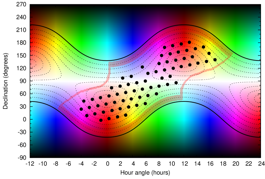
Figure 2: The sky in the first equatorial system, as it is seen by the RCC telescope mount used for the evaluation of the pointing models. The hue levels (in parallel with the horizontal axis) represent the celestial hour angle values while the luminance levels correspond to the celestial declination values. The distance in the color space is equivalent to the apparent celestial distance while the projected distance in this graph is proportional to the movements of the equatorial and declination axes. The clear white stripe is the distorted projection of the north celestial pole while the fully black stripe (at the bottom and the top) is the distorted projection of the south celestial pole. The horizon is shown by the two parallel thick black curves while the various positive horizontal elevation levels (in steps of $10^{\circ}$) are shown as thin black dashed curves. The mount domain is limited by the thick red stripe. These limits correspond both to the horizon as well as the northern pillar of the equatorial axis pier.

5 Implementation and model tests

In order to use the pointing model in practice, one should consider how it can be implemented for “real” telescopes. The actual implementation has to have two essential parts:

• First, one should obtain an appropriately chosen series of astrometric calibration frames of the given instrument in order to obtain the respective $(\tau_{n},\delta_{n})$ and $(T_{n},D_{n})$ values needed for the model. Afterwards, once these data are known, the parameters of the pointing model are needed to be fitted.

• Second, “implementation” also refers to the insertion of the model parameters into the telescope control system (TCS) in order to have a benefit during the observations.

In this section, we summarize our method of implementation, considering both the model parameter regression as well as the integration in a TCS.

5.1 Derivation of pointing model parameters

To implement our model, one should employ a classic, purely linear least squares regression analysis on functions containing merely linear combinations of trigonometric expressions. By considering the definitions of the linear least squares method ($\chi^{2}$, see Eq. 12) as well as the actual model (see Eq. 14), one could derive that the merit function needed to be minimized is

$$\chi^{2}=\sum\limits_{n=1}^{N}\left[\mathbf{p}_{L=\dots}(\tau_{n},\delta_{n})-\mathbf{p}(T_{n},D_{n})\right]^{2},$$ (36)

where

$$\mathbf{p}_{L=\dots}(\tau,\delta)=\mathbf{p}(\tau_{n},\delta_{n})+\sum\limits_{k=1}^{6}\sum\limits_{\ell=0}^{L}\sum\limits_{m=-\ell}^{\ell}a_{k\ell m}Y_{\ell m}(\tau,\delta)\mathbf{p}_{k}(\tau,\delta).$$ (37)

If $L=0$, we get the isotropic pointing model (having $6$ parameters in total) while for $L=1$ and $L=2$, we get the anisotropic cases with $22$ and $46$ free parameters. Of course, the value of $L$ can further be increased, however, one should keep in mind that additional identities similar to Eqs. (25)-(26) and/or Eqs. (27)-(32) will appear during the expansions.

Our current implementation for minimizing $\chi^{2}$ is based on shell scripts written in the language of bash. These scripts exploit standard UNIX text processing utilities as well as the lfit utility of the FITSH package (Pál, 2012). This implementation expects a four-column input file (where each line contains the $\tau_{n},\delta_{n},T_{n},D_{n}$ values) and it is available on the FITSH website in the “Examples” section.

5.2 Integration in telescope control systems

Once the pointing model parameters are known, they should be integrated in the TCS. However, such an integration needs a lower level access to the TCS software stack while the above described procedure for obtaining the coefficients can be done by anyone who has observational access to the telescope.

There are two ways to use the model:

• First, Eq. (14) (or Eq. 11 when considering only anisotropic models) should be evaluated when one computes the apparent equatorial coordinates based on the encoder values. This type of calculation is performed when the TCS is asked to report the current position, i.e. after the reading of the encoders on the mount axes.

• Second, the inverse form of Eq. (14) needs to be evaluated during pointing and tracking of the telescopes. Namely, if one has to determine the encoder values based on the apparent first equatorial coordinates. This type of calculation is performed when the TCS is commanded to slew the telescope to a certain position, i.e. before targeting the motors (and/or any mechanisms).

Any software library that handles pointing model evaluation needs to be ready for implementing both of the above types.

In practice, the inversion of Eq. (14) can be implemented by changing the sign in the series expansion coefficients. This type of inversion yields systematic offsets in the order of $a_{k\ell m}^{2}$. If the typical mount deflections are in the range of a few arcminutes (i.e. a milliradian), then the error caused by this improper inversion yields a systematic effect in the range of sub-arcsecond scale (i.e. microradians) which is usually sufficient. If higher accuracy is needed, the inversion can be done in a two-step iteration, yielding errors in the range of $a_{k\ell m}^{3}$. Since practical applications do not rely on subsequent evaluation of the pointing model corrections, these errors do not accumulate.

The above cited “Examples” section of the FITSH webpage contains a full implementation of an ANSI C library that can also be integrated in a TCS. In addition, this section of the webpage links some code snippets taken from the currently running version of an 1-m class telescope control software (see below the next subsection for more details).

Figure 3: Residuals of the pointing model applied to the Konkoly 1-meter RCC telescope. The left panel shows the respective components of the $\mathbf{p}_{L=0}(\tau_{n},\delta_{n})-\mathbf{p}(T_{n},D_{n})$ vectors for the isotropic case while the right panel shows these difference vector components for the $L=1$ anisotropic model. The scales for the difference vectors are the same for both panels: one degree in the main abscissa and ordinate refers to one arcsecond in the residual vector components. Note that the figures are redundant, not only because they show all of the $(x,y)$, $(y,z)$ and $(z,x)$ component combinations but due to the fact that residual vectors are always tangential to the unit sphere. The strong structure of systematics in the residual in the isotropic case is quite explicit. Note also that the residual vectors would be as large as the individual panels if we plot the residuals without any pointing model. See text for further details.

5.3 Model tests

In order to test the feasibility of our model we conducted a series of observations with the recently refurbished 1-meter Ritchey–Chrétien-coudé (RCC) telescope of the Konkoly Observatory. This telescope is installed on an English cross-axis mount. The northern pillar of this type of mount strictly limits the slew domain of the telescope within a certain range since the tube is unable to observe objects close to lower culmination. In the available telescope motion domain we defined a grid of ($\tau_{n},\delta_{n}$) values and exposures were taken on each grid point with a net time of 20 seconds. In total, we gathered 81 images covering the sky nearly uniformly with the inclusion of polar crossing. Due to the partially cloudy weather, only 69 of these images have successfully been analyzed in order to have accurate astrometric solutions. The positions of these measurements are displayed in Fig. 2. Images were acquired with an Andor iXon-888 frame-transfer electron-multiplying CCD camera (EMCCD) and reduced with the standard calibration procedures using the FITSH utilities (Pál, 2012). Since the net field-of-view of the optical setup is relatively small ($3.4^{\prime}\times 3.4^{\prime}$), astrometric solutions were derived using images acquired in parallel with a guider telescope. For an initial solution, we exploited the offline version of the Astrometry.net package (Lang et al., 2010) while the cross-matching of the two camera images as well as the final astrometric solutions were obtained with the appropriate tasks of the FITSH package using the USNO catalogue (Monet et al., 2003) as a reference.

After obtaining the J2000.0 centroids of each frame, apparent first equatorial coordinates (hour angle and declination) were obtained after correcting for precession, nutation, aberration and refraction using the standard procedures (Meeus, 1998; Wallace, 2008). The list of encoder positions read at the exposure midpoint was used as an input series of $(\tau_{n},\delta_{n})$ values while the corrected astrometric solutions were used as an input series of $(T_{n},D_{n})$ values.

The unbiased residuals of the isotropic, the first-order anisotropic and the second-order anisotropic pointing models were $\sigma_{0}=69.1\cdot 10^{-6}$, $\sigma_{1}=14.8\cdot 10^{-6}$ and $\sigma_{2}=10.2\cdot 10^{-6}$ radians, respectively (where $\sigma_{L}$ denotes the residuals corresponding to the $L$th order in the spherical harmonics expansion). Since one arcsecond is equal to $4.84814\cdot 10^{-6}$ radians, these values correspond to $14.2^{\prime\prime}$, $3.0^{\prime\prime}$ and $2.1^{\prime\prime}$. We note here that without any pointing model applied (which is similar to setting forcibly all of the coefficients $a_{k\ell m}$ to zero), the residual is $\sigma_{\emptyset}=0.0011$ radian, equivalent to $3.7^{\prime}$. This is $\approx 16$ times larger even than the residual corresponding to the isotropic ($L=0$) case. We plot the typical structures of pointing model residuals for the $L=0$ and $L=1$ case in the two panels of Fig. 3.

The fitted values and the respective uncertainties of the model coefficients can also be used to measure the actual deflections of the telescope. For instance, in our case the isotropic model yields values for the polar displacement and encoder zero point offsets that can be used for tuning the telescope. The actual values for the polar displacement are $a=0.000163\pm 0.000012$, $b=0.000356\pm 0.000010$ while the encoder zero points are $c^{\prime}=0.000844\pm 0.000013$ and $e^{\prime}=0.000705\pm 0.000009$ radians. It also turns out that the deviation of the two axes is also significant, being in the range of arcminute ($d=0.000315\pm 0.000085$). However, this value represents an average value for these deflections since the effects described in Sec. 4.2 can yield an anisotropy in any of the previously mentioned values. Indeed, for instance, the deviation of the two axes shows a clear dependence on the telescope position itself, namely the corresponding coefficients are $a_{400}=0.000573\pm 0.000091$, $a_{410}=-0.000008\pm 0.000023$, $a_{41,-1}=-0.000077\pm 0.000056$ and $a_{41,+1}=0.000191\pm 0.000056$ (also in radians). It means that the deflection of the two axes can vary with a full amplitude of at least $1.5$ arcminutes on the total telescope motion domain.

We also included two terms corresponding to the $G=240$ gear ratio of the hour axis worm-drive of the RCC telescope. This inclusion yielded a decrement of the unbiased $\chi^{2}$ values of $3.5$ (which should be compared to $2N-P=116$, where $N=69$, the number of the frames and $P=22$, the number of parameters in the $L=1$ anisotropic model). At the first glance, this fact might prove that the pointing model is improved by this additional term. However, compared to the total degrees of freedom, this decrement is marginal as well as the respective amplitude that differs from zero only by 1.5-sigma. In addition, total measured periodic error of this telescope is $\lesssim 0.15^{\prime\prime}$, which is well below the residuals of the model. All in all, we can conclude that this telescope cannot benefit with this inclusion, but other telescopes (e.g. amateur-class mechanics with typical periodic errors in the range of tens of arcseconds) might do so.

5.4 Polar crossing

It should be noted that spherical harmonics yield the same values while we observe the same celestial position before and after polar crossing. In other words, $Y_{\ell m}(\tau,\delta)=Y_{\ell m}(\tau+180^{\circ},180^{\circ}-\delta)$ for all values of $\tau$ and $\delta$. However, some anisotropic physical effects (see Sec. 4.2 above) might have different yields depending on the pier side of the telescope. Since the telescope can reach most of the target positions in both configurations, it is worth separating the coefficients corresponding to these two configuration domains. Here we define two target points to be in the same configuration if the telescope can be re-positioned between the two points without polar crossing.

The easiest way to do this is to consider points with $\delta\lesssim 90^{\circ}$ and $90^{\circ}\lesssim\delta$ in independent fits. Indeed, our analysis yields an unbiased residual of $1.6^{\prime\prime}$ and $1.7^{\prime\prime}$ for the $L=1$ model if the two parts of the sky are treated separately. Both residuals are significantly smaller than the residual of $3.0^{\prime\prime}$ and even a bit smaller than the $L=2$ model for the full coverage. If we perform this separation in the isotropic model, the unbiased residuals are going to be roughly the same (namely, $14.0^{\prime\prime}$ and $12.1^{\prime\prime}$, in our case).

6 Summary

In this paper we have presented a generic analytical anisotropic telescope pointing model derived from purely mathematical considerations. Our results show that this type of approach provides RMS residuals comparable and even better than earlier types of pointing models. It should be noted, however, that this pointing model does not account directly the temperature dependence of the telescope system. Based on earlier works (Mittag et al., 2008), the coefficients for the drifts of the various parameters due to the thermal expansion can be as large as $0.2-1^{\prime\prime}$ per degrees Celsius. Hence, the accuracy of the ambient temperature should be within a few degrees Celsius in order to recover the pointing with an accuracy comparable to the RMS residuals. Uncertainties in the refraction model, for instance a variation of $15\,{\rm hPa}$ in the pressure and/or $5$ degrees Celsius in the temperature yield an offset of $1^{\prime\prime}-2^{\prime\prime}$ even at moderate ($25-45$ degrees of) elevations above the horizon. Although an improper refraction model can be corrected via the $Y_{\ell m}$ functions, the correction factors depend on the temperature and/or the density profile of the layers in the atmosphere. A major advantage of our model is the lack of parameterization via polar coordinates. In our tests, one of the grid points had a declination of $\delta_{\rm J2000}=89^{\circ}55^{\prime}$ and it is also a well behaved point, not an outlier – despite the fact that the respective value of $1/\cos\delta$ is more than $700$. In order to have a successful implementation for our model, one should employ only classic linear least squares regression analysis on functions containing purely trigonometric expressions. The implementation of both the model fit and the model evaluation functions is straightforward, and is demonstrated on the FITSH webpage.