Abstract

This paper gives a rigorous proof of a conjectured statistical self-similarity property of the eigenvalues random matrices from the Circular Unitary Ensemble. We consider on the one hand the eigenvalues of an $n\times n$ CUE matrix, and on the other hand those eigenvalues $e^{i\phi}$ of an $mn\times mn$ CUE matrix with $\left|\phi\right|\leq\pi/m$, rescaled to fill the unit circle. We show that for a large range of mesoscopic scales, these collections of points are statistically indistinguishable for large $n$. The proof is based on a comparison theorem for determinantal point processes which may be of independent interest.

title = Self-Similarity in the Circular Unitary Ensemble, author = Elizabeth S. Meckes and Mark W. Meckes, plaintextauthor = Elizabeth S. Meckes, Mark W. Meckes, keywords = random unitary matrices, Haar measure, eigenvalues, self-similarity, determinantal point processes, year=2016, number=9, received=20 October 2015, revised=10 June 2016, published=15 June 2016, doi=10.19086/da.736,

[classification=text]

1 Introduction

The set of $N\times N$ unitary matrices is a compact Lie group, and as such, possesses a unique probability measure which is invariant under left- and right-translation (called Haar measure). In random matrix theory, the unitary group together with Haar probability measure is called the circular unitary ensemble (CUE). The word circular refers to the fact that all of the eigenvalues of a CUE matrix lie on the unit circle in the complex plane.

There has long been a folklore conjecture that the distribution of the eigenvalues of a CUE random matrix has a self-similar structure. For example, in their statistical analysis [3] of CUE eigenvalues and zeroes of the Riemann zeta function, Coram and Diaconis hypothesized that the following may hold:

Conjecture 1.

Let $U$ be an $N\times N$ random matrix from the CUE with eigenvalues $\{e^{i\theta_{j}}\}_{1\leq j\leq N}$, where $0\leq\theta_{1}\leq\dots\leq\theta_{N}<2\pi$. Choose an eigenvalue $e^{i\theta_{K}}$ uniformly, and let $T$ be the length of the counter-clockwise circular arc from $\theta_{K}$ to $\theta_{K+k}$, where the indices are interpreted modulo $N$. Let $\phi\in[0,2\pi)$ be a uniformly chosen random angle, independent of $U$. If $k$ and $N$ are both large, then the random set of points

$$\left\{e^{i\left(\phi+\frac{2\pi\theta_{j}}{T}\right)}\right\}_{K\leq j<K+k}$$

is statistically indistinguishable from the eigenvalues of a $k\times k$ random matrix from the CUE.

That is, a random choice of $k$ sequential eigenvalues of an $N\times N$ CUE matrix $U$, rescaled and randomly rotated, is indistinguishable from the full set of eigenvalues of a $k\times k$ random matrix.

Aside from statistical evidence for the conjecture, there is a result of E. Rains [15] which is suggestive of this kind of self-similarity. Suppose that $U$ is an $N\times N$ random CUE matrix, with $N=nk$; Rains proved that the distribution of the eigenvalues of $U^{n}$ is exactly that of the collection of eigenvalues of $n$ independent $k\times k$ random CUE matrices. That is, wrapping the eigenvalues of $U$ around the circle $n$ times produces $n$ independent copies of the $k$ eigenvalues of a $k\times k$ random matrix. It is tempting to view each of those collections of $k$ eigenvalues as coming from one of the $n$ arcs of the circle that gets stretched to cover the circle once (this is not at all the way Rains’ theorem is actually proved). If this intuition were correct, it would illustrate exactly the kind of self-similarity conjectured by Coram and Diaconis.

In this paper, we give a rigorous proof of a version of the self-similarity conjecture. The following notation is used throughout. Let $U$ be an $n\times n$ random CUE matrix with eigenvalues $\{e^{i\theta_{j}}\}_{1\leq j\leq n}$, with $\theta_{j}\in[-\pi,\pi)$ for each $j$. (It is a matter of technical convenience to take the arguments of the eigenvalues to be in $[-\pi,\pi)$ here instead of in $[0,2\pi)$ as in Conjecture 1.) For $A\subseteq[-\pi,\pi)$, $\mathcal{N}_{n,A}$ denotes the number of eigenangles $\theta_{j}$ which lie in $A$; we generally omit the $n$ and write $\mathcal{N}_{A}$. For $\theta\in[0,\pi)$, $\mathcal{N}_{[-\theta,\theta]}$ is denoted by $\mathcal{N}_{\theta}$. For $m\geq 1$, let $U^{(m)}$ be an $nm\times nm$ random CUE matrix with eigenvalues $\{e^{i\phi_{j}}\}_{1\leq j\leq nm}$, with $\phi_{j}\in[-\pi,\pi)$ for each $j$, and let

$$\mathcal{N}_{n,A}^{(m)}=\mathcal{N}_{A}^{(m)}:=\#\left\{j\mathrel{}\middle|\mathrel{}\phi_{j}\in\left[-\frac{\pi}{m},\frac{\pi}{m}\right),\ m\phi_{j}\in A\right\};$$

$\mathcal{N}_{A}^{(m)}$ counts the random points in $A$ of the point process consisting of the eigenvalues of $U^{(m)}$ in the arc of length $\frac{2\pi}{m}$ about $1$, and rescaling to fill out the whole circle. While the total number of eigenvalues in this arc is random, it concentrates strongly at its expected value of $n$. In the context of the Diaconis–Coram conjecture, our $nm$ plays the role of $N$ and $n$ plays the role of $k$.

Theorem 2.

Suppose that $m,n\geq 1$, and that $A\subseteq[-\pi,\pi)$ has diameter $\operatorname{diam}A\leq\pi$. Then

$$d_{TV}\left(\mathcal{N}_{A},\mathcal{N}^{(m)}_{A}\right)\leq W_{1}\left(\mathcal{N}_{A},\mathcal{N}^{(m)}_{A}\right)\leq\frac{\sqrt{mn}\left|A\right|\operatorname{diam}A}{6\pi},$$

where $d_{TV}(\cdot,\cdot)$ denotes total variation distance between random variables, $W_{1}(\cdot,\cdot)$ denotes $L^{1}$-Wasserstein distance, and $\left|A\right|$ denotes the Lebesgue measure of $A$.

For context, recall that $\mathbb{E}\mathcal{N}_{A}=\frac{n\left|A\right|}{2\pi}$; the same is true for $\mathcal{N}_{A}^{(m)}$.

In the statement of Theorem 2, and all of the following results, precise constants are included for concreteness, with no claims as to their sharpness. The definitions of $d_{TV}(\cdot,\cdot)$ and $W_{1}(\cdot,\cdot)$ are recalled at the end of this section.

Theorem 2 was stated with the implicit assumption that $m$ is an integer, since it is in that case that it relates directly to Conjecture 1. However, it is only strictly necessary that $mn$ is an integer, and a slight refinement of the proof shows that for any $m\geq 1$, if $mn\in\mathbb{N}$, then

$$d_{TV}\left(\mathcal{N}_{A},\mathcal{N}^{(m)}_{A}\right)\leq W_{1}\left(\mathcal{N}_{A},\mathcal{N}^{(m)}_{A}\right)\leq C\left(1-\frac{1}{m^{2}}\right)\sqrt{mn}\left|A\right|\operatorname{diam}A.$$ (1)

In particular, this yields the comparison

$$d_{TV}\left(\mathcal{N}_{n,A},\mathcal{N}_{n+1,\frac{n}{n+1}A}\right)\leq W_{1}\left(\mathcal{N}_{n,A},\mathcal{N}_{n+1,\frac{n}{n+1}A}\right)\leq C\frac{\left|A\right|\operatorname{diam}A}{\sqrt{n}}$$

between $n\times n$ CUE eigenvalues and $(n+1)\times(n+1)$ CUE eigenvalues.

As a consequence of Theorem 2, if $\{A_{n}\}$ is a sequence of sets such that either $\operatorname{diam}A_{n}=o(n^{-1/4})$ or $\left|A_{n}\right|=o(n^{-1/2})$ as $n\to\infty$, then

$$d_{TV}\left(\mathcal{N}_{A_{n}},\mathcal{N}^{(m)}_{A_{n}}\right),W_{1}\left(\mathcal{N}_{A_{n}},\mathcal{N}^{(m)}_{A_{n}}\right)\to 0.$$

Thus indeed, a sequential arc of about $n$ of the $nm$ eigenvalues of an $nm\times nm$ random matrix is statistically indistinguishable, on the scale of $o(n^{-1/4})$ for diameter or $o(n^{-1/2})$ for Lebesgue measure, from the $n$ eigenvalues of an $n\times n$ random matrix.

A remarkable feature of Theorem 2 is that it yields microscopic information even at a mesoscopic scale: if $\frac{1}{n}\ll\operatorname{diam}A_{n}\ll\frac{1}{n^{1/4}}$, then $\mathcal{N}_{A_{n}}$ and $\mathcal{N}^{(m)}_{A_{n}}$ both have expectations and variances tending to infinity (as follows from Lemma 7 below). One would thus typically try to understand the point processes at these scales by studying statistical properties of the recentered and rescaled counts, rather than try to observe individual points. Here, we are able to make direct point-by-point comparisons of the two point processes treated as discrete objects, with no rescaling or continuous approximations.

The fact that we are able to compare the two point processes with no rescaling certainly suggests that we are witnessing a true self-similarity phenomenon which is a special feature of the structure of the eigenvalues of CUE random matrices. However, one should be careful to check that the two point processes are not similar simply because they have the same limit. Indeed, Wieand [19] and Soshnikov [17] showed that

$$\frac{\mathcal{N}_{\theta}-\mathbb{E}\mathcal{N}_{\theta}}{\sqrt{\operatorname{Var}\mathcal{N}_{\theta}}}\Rightarrow N(0,1)$$

as $n\to\infty$ for fixed $\theta$; the same then follows for $\mathcal{N}_{\theta}^{(m)}$. Figure 1 gives a convincing visual illustration that $\mathcal{N}_{A}$ and $\mathcal{N}_{A}^{(m)}$ resemble each other more closely than either resembles a Gaussian distribution; a rigorous proof of this fact is given in Proposition 8 below.

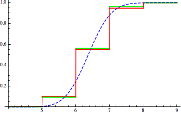
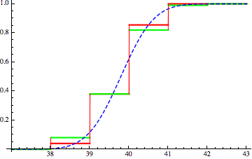
Kolmogorov–Smirnov statistics
$\mathcal{N}_{0.2}$ to Gaussian	0.329
$\mathcal{N}^{(2)}_{0.2}$ to Gaussian	0.319
$\mathcal{N}_{0.2}$ to $\mathcal{N}^{(2)}_{0.2}$	0.016

Kolmogorov–Smirnov statistics
$\mathcal{N}_{0.25}$ to Gaussian	0.262
$\mathcal{N}^{(2)}_{0.25}$ to Gaussian	0.262
$\mathcal{N}_{0.25}$ to $\mathcal{N}^{(2)}_{0.25}$	0.04

Figure 1: Left: Simulated cumulative distribution functions (500 trials) for $\mathcal{N}_{0.2}$ (red) and $\mathcal{N}^{(2)}_{0.2}$ (green), with $n=100$.
Right: Simulated cumulative distribution functions (200 trials) for $\mathcal{N}_{0.25}$ (red) and $\mathcal{N}^{(2)}_{0.25}$ (green), with $n=500$.
The dotted lines show Gaussian cumulative distribution functions with mean equal to the theoretical mean of both $\mathcal{N}_{\theta}$ and $\mathcal{N}^{(2)}_{\theta}$ (i.e., $\frac{20}{\pi}\approx 6.4$ and $\frac{125}{\pi}\approx 39.8$, respectively) and variance equal to the average of the two corresponding sample variances.

We conjecture that a comparable result to Theorem 2 holds without the restriction on $\operatorname{diam}A$, and that the factor of $\sqrt{n}$ in the right hand side is an artifact of our proof; this would imply that $\mathcal{N}_{A_{n}}$ and $\mathcal{N}_{A_{n}}^{(m)}$ become indistinguishable as long as $\left|A_{n}\right|\to 0$. For more details, see the remark at the end of Section 2. On the other hand, we do not expect such a result to hold for sets of constant size; i.e., independent of $n$. For example, Rains [14] gives precise asymptotics for $\operatorname{Var}\mathcal{N}_{\theta}$ for $n\to\infty$ and $\theta$ fixed, which show that $\operatorname{Var}\mathcal{N}_{\theta}$ and $\operatorname{Var}\mathcal{N}_{\theta}^{(m)}$ are not asymptotically equal. This suggests (but does not formally imply) that Theorem 2 does not hold in this setting. Rains’ estimate does show that Proposition 9 below on the asymptotic equality of variances does not extend to that regime.

We expect that a version of Theorem 2 holds for the other circular ensembles of random matrix theory; however, our approach is via the determinantal structure of the eigenvalue process for the CUE, which is not present outside the unitary case.

Finally, some comments on the relationship between Conjecture 1 and Theorem 2 are in order. The models of self-similarity being used are not identical; in Conjecture 1, exactly $k+1$ sequential eigenvalues are selected and stretched as needed to make the first and last meet, resulting in exactly $k$ random points. In Theorem 2, the eigenvalues from an arc making up a fixed fraction of the circle are chosen and that arc is stretched (deterministically) to cover the whole circle; the resulting total number of points is random. However, in the mesoscopic regime the two models are essentially the same. The idea is the following: eigenvalue rigidity (see Lemma 10 of [12]) implies that the difference between the $j^{\mathrm{th}}$ and the $(j+n)^{\mathrm{th}}$ eigenangles of an $nm\times nm$ CUE matrix is about $\frac{2\pi}{m}+O\bigl{(}\frac{\sqrt{\log n}}{n}\bigr{)}$ with high probability. So whereas Theorem 2 considers the eigenangles of an $nm\times nm$ matrix in an interval of length $\theta/m$, Conjecture 1 suggests considering the eigenangles in an interval whose length is random but typically about $\frac{\theta}{m}+\theta O\bigl{(}\frac{\sqrt{\log n}}{n}\bigr{)}$. But if $\theta\ll\frac{1}{\sqrt{\log n}}$, then with extremely high probability an interval of length $\theta\frac{\sqrt{\log n}}{n}$ contains no eigenangles, and so the corresponding counts are the same.

The rest of this paper is organized as follows. In Section 2 we give the background and general results on determinantal point processes needed to prove Theorem 2, followed by the proof of the theorem and a corollary giving a rate for the classical convergence of the eigenvalue process to the sine kernel process on a microscopic scale. In Section 3 we give precise asymptotics for the variances of the counting functions. As a consequence, we are able to identify a sharp rate of convergence in the central limit theorem mentioned above, which is in particular much slower than the merging of distributions in Theorem 2. We also show that the variances of the counting functions of the two processes are asymptotically equal throughout the entire mesoscopic regime, giving a rigorous proof of another manifestation of the self-similarity phenomenon. Finally, Section 4 gives a surprising comparison between the joint intensities of the eigenvalues processes for $U$ and $U^{(m)}$.

We conclude this section with a brief review of the notions of distance used here. The following distances can be defined much more generally, but for our purposes, it suffices to define them for integer-valued random variables $X$ and $Y$.

1. The total variation distance from $X$ to $Y$ is defined by

   $$d_{TV}(X,Y):=\sup_{A\subseteq\mathbb{Z}}\left|\mathbb{P}[X\in A]-\mathbb{P}[Y\in A]\right|.$$

2. The $L^{1}$-Wasserstein distance is defined by

   $$W_{1}(X,Y):=\inf_{(Z_{1},Z_{2})}\mathbb{E}\left|Z_{1}-Z_{2}\right|,$$

   where the infimum is over random vectors $(Z_{1},Z_{2})$ such that $Z_{1}$ has the same distribution as $X$ and $Z_{2}$ has the same distribution as $Y$ (such a random vector is called a coupling of $X$ and $Y$).

   The Kantorovich–Rubenstein Theorem states that $W_{1}$ can equivalently be defined as

   $$W_{1}(X,Y):=\sup_{f}\left|\mathbb{E}f(X)-\mathbb{E}f(Y)\right|,$$

   where the supremum is over 1-Lipschitz functions $f:\mathbb{Z}\to\mathbb{R}$. The distance $W_{1}$ is a metric for the topology of weak convergence plus convergence of absolute first moments. (See [18, Section 6] for a thorough discussion and proofs.)

Note that an indicator function of a set $A$ of integers is 1-Lipschitz on $\mathbb{Z}$, and so for $X$ and $Y$ integer-valued,

$$d_{TV}(X,Y)\leq W_{1}(X,Y).$$ (2)

2 Determinantal point processes and the proof of Theorem 2

Let $\Lambda$ be a locally compact Polish space. A simple point process on $\Lambda$ is a random integer-valued (positive) Radon measure $\chi$ on $\Lambda$, such that the measure of any singleton is at most $1$. Alternatively, it may be viewed as a locally finite random set of points in $\Lambda$; if $A\subseteq\Lambda$ then we write $\mathcal{N}_{A}=\chi(A)$ for the (random) number of points lying in $A$. If $\Lambda$ is equipped with a reference Borel measure $\mu$, then the $k^{\mathrm{th}}$ joint intensity or correlation function $\rho_{k}:\Lambda^{k}\to[0,\infty)$ of $\chi$ is defined by the equation

$$\mathbb{E}\left[\prod_{i=1}^{k}\mathcal{N}_{A_{i}}\right]=\int_{A_{1}}\dots\int_{A_{k}}\rho_{k}(x_{1},\dots,x_{k})\ d\mu(x_{1})\dots d\mu(x_{k}),$$

whenever $A_{1},\dots,A_{k}\subseteq\Lambda$ are measurable and pairwise disjoint, assuming that such functions exist. A simple point process is called a determinantal point process with kernel $K:\Lambda^{2}\to\mathbb{C}$ if its joint intensities exist and

$$\rho_{k}(x_{1},\dots,x_{k})=\det\left[K(x_{i},x_{j})\right]_{i,j=1}^{k}.$$

Note that it is immediate from the definition that the restriction of a determinantal point process on $\Lambda$ to a measurable subset $D\subseteq\Lambda$ is again a determinantal point process.

A kernel $K:\Lambda^{2}\to\mathbb{C}$ defines an integral operator on $L^{2}(\mu)$ by

$$\mathcal{K}(f)(x):=\int_{\Lambda}K(x,y)f(y)d\mu(y);$$ (3)

if $K(x,y)=\overline{K(y,x)}$, then the operator $\mathcal{K}$ is self-adjoint. It was proved by Macchi [11] and Soshnikov [16] that a kernel $K$ which defines a self-adjoint, trace class operator $\mathcal{K}$ as above is the kernel of a determinantal point process if and only if all of the eigenvalues of $\mathcal{K}$ lie in $[0,1]$.

For the remainder of this paper, $\chi$ will denote the point process of eigenvalue angles in $[-\pi,\pi)$ of an $n\times n$ CUE random matrix. For fixed $m\geq 1$, let $\chi^{(m)}$ denote the point process obtained by multiplying by $m$ those eigenvalue angles of an $nm\times nm$ CUE random matrix which lie in $\bigl{[}-\frac{\pi}{m},\frac{\pi}{m}\bigr{)}$.

It is a fact originally due to Dyson that $\chi$ is a determinantal point process on $[-\pi,\pi)$; it follows easily that $\chi^{(m)}$ is as well. The following Proposition gives explicit formulae for the corresponding kernels.

Proposition 3.

The point process $\chi^{(m)}$ on $[0,2\pi)$ is determinantal with kernel

$$K_{n}^{(m)}(x,y)=\frac{1}{2\pi}\frac{\sin\left(\frac{n(x-y)}{2}\right)}{m\sin\left(\frac{(x-y)}{2m}\right)}.$$

with respect to Lebesgue measure.

Proof.

The case $m=1$ was proved by Dyson in [5] (although that work predates the language of determinantal point processes); see also [13, Section 11.1] or [10, Section 5.4]. The general case follows from a change of variables which shows that $K_{n}^{(m)}(x,y)=\frac{1}{m}K_{mn}^{(1)}\bigl{(}\frac{x}{m},\frac{y}{m}\bigr{)}$. ∎

Note in particular that the corresponding operators $\mathcal{K}_{n}^{(m)}$ as defined in (3) are self-adjoint and trace class.

The following general result on determinantal point processes is the main technical ingredient behind Theorem 2.

Proposition 4.

Let $\mathcal{N}$ and $\widetilde{\mathcal{N}}$ be the total numbers of points in two determinantal point processes on $(\Lambda,\mu)$ with conjugate-symmetric kernels $K,\widetilde{K}\in L^{2}(\mu\otimes\mu)$, respectively. Suppose that $\mathcal{N},\widetilde{\mathcal{N}}\leq N$ almost surely. Then

$$d_{TV}(\mathcal{N},\widetilde{\mathcal{N}})\leq W_{1}(\mathcal{N},\widetilde{\mathcal{N}})\leq\sqrt{N\int\int\left|K(x,y)-\widetilde{K}(x,y)\right|^{2}\ d\mu(x)d\mu(y)}.$$

Proposition 4 depends on the following remarkable property of determinantal point processes.

Lemma 5 ([8, Theorem 7]).

Consider a determinantal point process with kernel $K$, whose corresponding integral operator $\mathcal{K}$ is self-adjoint and trace class, with eigenvalues $\{\lambda_{j}\}$. Let $\mathcal{N}$ be the total number of points in the process. Then

$$\mathcal{N}\stackrel{{\scriptstyle d}}{{=}}\sum_{j}\xi_{j},$$

where $\{\xi_{j}\}$ are independent Bernoulli random variables with $\mathbb{P}[\xi_{j}=1]=\lambda_{j}$ and $\mathbb{P}[\xi_{j}=0]=1-\lambda_{j}$.

Proof of Proposition 4.

By (2), it suffices to prove the second inequality.

Let $\{\lambda_{j}\}$ and $\{\widetilde{\lambda}_{j}\}$ be the eigenvalues, listed in nonincreasing order, of the integral operators $\mathcal{K}$ and $\widetilde{\mathcal{K}}$ with kernels $K$ and $\widetilde{K}$ respectively. Since $\mathcal{N},\widetilde{\mathcal{N}}\leq N$, by Lemma 5, $\lambda_{j}=\widetilde{\lambda}_{j}=0$ for $j>N$. Let $\{Y_{j}\}_{j=1}^{N}$ be independent random variables uniformly distributed in $[0,1]$. For each $j$, define

$$\xi_{j}=\mathbbm{1}_{Y_{j}\leq\lambda_{j}}\qquad\text{and}\qquad\widetilde{\xi}_{j}=\mathbbm{1}_{Y_{j}\leq\widetilde{\lambda}_{j}}.$$

Through Lemma 5, this gives a coupling of $\mathcal{N}$ and $\widetilde{\mathcal{N}}$, and so

$$W_{1}(\mathcal{N},\widetilde{\mathcal{N}})\leq\mathbb{E}\left|\sum_{j=1}^{N}\xi_{j}-\sum_{j=1}^{N}\widetilde{\xi}_{j}\right|\leq\sum_{j=1}^{N}\mathbb{E}\left|\xi_{j}-\widetilde{\xi}_{j}\right|=\sum_{j=1}^{N}\left|\lambda_{j}-\widetilde{\lambda}_{j}\right|\leq\sqrt{N\sum_{j=1}^{N}\left|\lambda_{j}-\widetilde{\lambda}_{j}\right|^{2}}.$$ (4)

By the Hoffmann–Wielandt inequality [9, Theorem II.6.11],

$$\sqrt{\sum_{j=1}^{N}\left|\lambda_{j}-\widetilde{\lambda}_{j}\right|^{2}}\leq\left\|\mathcal{K}-\widetilde{\mathcal{K}}\right\|_{H.S.},$$

where $\lVert\cdot\rVert_{H.S.}$ denotes the Hilbert–Schmidt norm. The result now follows from the general fact that the Hilbert–Schmidt norm of an integral operator on $L^{2}(\mu)$ is given by the $L^{2}(\mu\otimes\mu)$ norm of its kernel (see e.g. [20, p. 245]). ∎

We are now in a position to prove the main theorem.

Proof of Theorem 2.

For every $0\leq\varphi\leq\frac{\pi}{2}$,

$$\varphi-\frac{1}{6}\varphi^{3}\leq\sin\varphi\leq m\sin\left(\frac{\varphi}{m}\right)\leq\varphi,$$ (5)

and so

$$0\leq\frac{1}{\sin\varphi}-\frac{1}{m\sin\left(\frac{\varphi}{m}\right)}\leq\frac{1}{\varphi-\frac{1}{6}\varphi^{3}}-\frac{1}{\varphi}\\ =\frac{\varphi}{6-\varphi^{2}}\leq\frac{\varphi}{3}.$$

Thus by Propositions 3 and 4,

$$\begin{split}W_{1}(\mathcal{N}_{A},\mathcal{N}^{(m)}_{A})&\leq\sqrt{\frac{mn}{(2\pi)^{2}}\int_{A}\int_{A}\sin^{2}\left(\frac{n(x-y)}{2}\right)\left(\frac{1}{\sin\left(\frac{x-y}{2}\right)}-\frac{1}{m\sin\left(\frac{x-y}{2m}\right)}\right)^{2}\ dx\ dy}\\ &\leq\frac{1}{6\pi}\sqrt{mn\int_{A}\int_{A}(x-y)^{2}\ dx\ dy}\\ &\leq\frac{1}{6\pi}\sqrt{mn}\left|A\right|\operatorname{diam}A.\qed\end{split}$$

The refinement (1) of Theorem 2 follows by using a higher-order Taylor expansion in (5).

Both $\mathcal{N}_{A}$ and $\mathcal{N}_{A}^{(m)}$ satisfy central limit theorems in the mesoscopic regime (see Proposition 8 and the remark which follows). We show in the next section that Theorem 2 does indeed describe a non-trivial self-similarity phenomenon on a mesoscopic level, which is not the result of both processes having the same limit.

In the microscopic regime, one can say more. As was first observed in [5], and more clearly spelled out in [13], the kernel $K_{n}^{(1)}=K_{n}$ has the following microscopic scaling limit:

$$\lim_{n\to\infty}\frac{2\pi}{n}K_{n}\left(\frac{2\pi x}{n},\frac{2\pi y}{n}\right)=\frac{\sin\bigl{(}\pi(x-y)\bigr{)}}{\pi(x-y)}.$$ (6)

The same microscopic scaling limit appears for bulk eigenvalues of certain Hermitian random matrices as well; see [1, 4, 13]. There is sufficient uniformity in the convergence in (6) to imply that the point process $\chi$, rescaled to lie in $[-n/2,n/2)$, converges as $n\to\infty$ to an unbounded point process on $\mathbb{R}$ which is determinantal, with the right hand side of (6) as its kernel with respect to Lebesgue measure. This process is called the sine kernel process; we denote by $\mathcal{S}_{A}$ the number of points of the sine kernel process which lie in $A\subseteq\mathbb{R}$. In particular, by e.g. [1, Lemma 4.2.48], $\mathcal{N}_{n,\frac{2\pi}{n}A}\Rightarrow\mathcal{S}_{A}$. A limited version of Theorem 2 can be deduced from the convergence to the sine kernel process. On the other hand, Theorem 2 actually improves on the classical microscopic result by estimating a rate of convergence, as follows.

Corollary 6.

Let $A\subseteq\mathbb{R}$, and let $\mathcal{S}_{A}$ denote the number of points of the sine kernel process which lie in $A$. Then

$$d_{TV}\bigl{(}\mathcal{N}_{\frac{2\pi}{n}A},\mathcal{S}_{A}\bigr{)}\leq W_{1}\bigl{(}\mathcal{N}_{\frac{2\pi}{n}A},\mathcal{S}_{A})\bigr{)}\leq\frac{5\left|A\right|\operatorname{diam}A}{n^{3/2}}$$

for all sufficiently large $n$.

Proof.

Let $n$ be large enough that $A\subseteq\left[-\frac{n}{2},\frac{n}{2}\right)$ and $\operatorname{diam}A\leq\frac{n}{2}$. Let $k\geq 0$. Recall that by definition of $\chi^{(2)}$,

$$\mathcal{N}^{(2)}_{2^{k}n,\frac{2\pi}{2^{k}n}A}=\mathcal{N}_{2^{k+1}n,\frac{2\pi}{2^{k+1}n}A}.$$

It thus follows from Theorem 2 (with $m=2$ and $2^{k}n$ in place of $n$) that

$$W_{1}\left(\mathcal{N}_{2^{k}n,\frac{2\pi}{2^{k}n}A},\mathcal{N}_{2^{k+1}n,\frac{2\pi}{2^{k+1}n}A}\right)\leq\frac{\sqrt{2^{k+1}n}}{6\pi}\frac{4\pi^{2}\left|A\right|\operatorname{diam}A}{(2^{k}n)^{2}}=\frac{2\sqrt{2}\pi\left|A\right|\operatorname{diam}A}{3(2^{k}n)^{3/2}}.$$

Fixing $M\in\mathbb{N}$ and applying this estimate for each $k\in\{0,\ldots,M-1\}$ then gives that

$$\begin{split}W_{1}\left(\mathcal{N}_{\frac{2\pi}{n}A},\mathcal{S}_{A}\right)&\leq\sum_{k=0}^{M-1}W_{1}\left(\mathcal{N}_{2^{k}n,\frac{2\pi}{2^{k}n}A},\mathcal{N}_{2^{k+1}n,\frac{2\pi}{2^{k+1}n}A}\right)+W_{1}\left(\mathcal{N}_{2^{M}n,\frac{2\pi}{2^{M}n}A},\mathcal{S}_{A}\right)\\ &\leq\frac{2\sqrt{2}\pi\left|A\right|\operatorname{diam}A}{3n^{3/2}}\sum_{k=0}^{M-1}\frac{1}{2^{3k/2}}+W_{1}\left(\mathcal{N}_{2^{M}n,\frac{2\pi}{2^{M}n}A},\mathcal{S}_{A}\right).\end{split}$$ (7)

As was discussed above, it is well known that $\mathcal{N}_{2^{M}n,\frac{2\pi}{2^{M}n}A}\Rightarrow\mathcal{S}_{A}$ as $M\to\infty$. Since all of the $\mathcal{N}_{2^{M}n,\frac{2\pi}{2^{M}n}A}$ and $\mathcal{S}_{A}$ are nonnegative random variables with means equal to $\left|A\right|$, weak convergence is equivalent to $W_{1}$ convergence, and so $W_{1}\left(\mathcal{N}_{2^{M}n,\frac{2\pi}{2^{M}n}A},\mathcal{S}_{A}\right)\to 0$ as $M\to\infty$. Thus taking the limit $M\to\infty$ in (7) yields

$$W_{1}\left(\mathcal{N}_{\frac{2\pi}{n}A},\mathcal{S}_{A}\right)\leq\frac{2\sqrt{2}\pi\left|A\right|\operatorname{diam}A}{3n^{3/2}}\sum_{k=0}^{\infty}\frac{1}{2^{3k/2}}\leq\frac{5\left|A\right|\operatorname{diam}A}{n^{3/2}}.\qed$$

Remark.

The application of the Cauchy–Schwarz inequality in the last step of (4) in the proof of Proposition 4 above is the source of the factor of $\sqrt{n}$ in the statement of Theorem 2, which we conjecture to be unnecessary. A direct estimate of the quantity

$$\sum_{j=1}^{N}\left|\lambda_{j}-\widetilde{\lambda}_{j}\right|,$$

which is bounded by the trace class norm of the difference $\mathcal{K}-\widetilde{\mathcal{K}}$, could potentially avoid that dimensional factor, thereby increasing the size of the mesoscopic regime in which Theorem 2 gives non-trivial information. Unfortunately, trace class norms are considerably more difficult to compute than Hilbert–Schmidt norms, and we have not found an estimate which improves on the approach taken above.

3 Some further asymptotics

The following lemma gives asymptotics for $\operatorname{Var}\mathcal{N}_{\theta}^{(m)}$ in various regimes. As was mentioned in the introduction, the paper [14] gives precise asymptotics as $n\to\infty$ for $\operatorname{Var}\mathcal{N}_{\theta}$ when $\theta$ is fixed, but in the present context, estimates for when $\theta$ varies with $n$ are needed.

Lemma 7.

Let $m\in\mathbb{N}$ be fixed. Whenever $\frac{3\pi}{2n}\leq\theta\leq\frac{\pi}{2}$,

$$\operatorname{Var}\mathcal{N}_{\theta}^{(m)}\geq\frac{1}{3\pi^{2}}\log\left(\frac{2n\theta}{3\pi}\right).$$

Moreover,

$$\operatorname{Var}\mathcal{N}_{\theta}^{(m)}\leq\begin{cases}\frac{n^{2}\theta^{2}+2}{4}&\text{if }0<\theta\leq\frac{1}{n},\\ \frac{1}{2}\log\bigl{(}e^{3/2}n\theta\bigr{)}&\text{if }\frac{1}{n}\leq\theta\leq\frac{\pi}{2}.\end{cases}$$

Consequently, for a sequence $\left\{\theta_{n}\in\left(0,\frac{\pi}{2}\right]\right\}$,

$$\operatorname{Var}\mathcal{N}_{n,\theta_{n}}^{(m)}\to\infty\qquad\text{if and only if}\qquad n\theta_{n}\to\infty.$$

Proof.

Observe that $\mathcal{N}_{n,[-\theta,\theta]}^{(m)}$ has the same distribution as $\mathcal{N}^{(1)}_{mn,[-\theta/m,\theta/m]}=\mathcal{N}_{mn,[-\theta/m,\theta/m]}$; since $m$ is fixed (i.e., independent of $n$), it therefore suffices to prove the estimates for $m=1$. Using general formulae for determinantal point processes, it is shown in the proof of [12, Proposition 8] that

$$\operatorname{Var}\mathcal{N}_{\theta}=\frac{1}{2\pi^{2}}\left[\int_{0}^{2\theta}\frac{z\sin^{2}\left(\frac{nz}{2}\right)}{\sin^{2}\left(\frac{z}{2}\right)}\ dz+2\theta\int_{2\theta}^{\pi}\frac{\sin^{2}\left(\frac{nz}{2}\right)}{\sin^{2}\left(\frac{z}{2}\right)}\ dz\right].$$ (8)

Now suppose that $\frac{3\pi}{2n}\leq\theta\leq\frac{\pi}{2}$. If $z\geq\varepsilon\geq\frac{2\pi}{n}$, then $z-\frac{\pi}{n}\geq\frac{z}{2}$, and so

$$\int_{\varepsilon}^{2\theta}\frac{\sin^{2}\left(\frac{nz}{2}\right)}{z}\ dz =\int_{\varepsilon}^{2\theta}\frac{1-\cos^{2}\left(\frac{nz}{2}\right)}{z}\ dz$$

$$=\log\left(\frac{2\theta}{\varepsilon}\right)-\int_{\varepsilon}^{2\theta}\frac{\sin^{2}\left(\frac{nz}{2}+\frac{\pi}{2}\right)}{z}\ dz$$

$$=\log\left(\frac{2\theta}{\varepsilon}\right)-\int_{\varepsilon+\frac{\pi}{n}}^{2\theta+\frac{\pi}{n}}\frac{\sin^{2}\left(\frac{nz}{2}\right)}{z-\frac{\pi}{n}}\ dz$$

$$\geq\log\left(\frac{2\theta}{\varepsilon}\right)-\int_{2\theta}^{2\theta+\frac{\pi}{n}}\frac{\sin^{2}\left(\frac{nz}{2}\right)}{z-\frac{\pi}{n}}\ dz-\int_{\varepsilon}^{2\theta}\frac{\sin^{2}\left(\frac{nz}{2}\right)}{z-\frac{\pi}{n}}\ dz$$

$$\geq\log\left(\frac{2\theta}{\varepsilon}\right)-\int_{2\theta}^{2\theta+\frac{\pi}{n}}\frac{1}{z-\frac{\pi}{n}}\ dz-2\int_{\varepsilon}^{2\theta}\frac{\sin^{2}\left(\frac{nz}{2}\right)}{z}\ dz$$

$$=\log\left(\frac{2\theta-\frac{\pi}{n}}{\varepsilon}\right)-2\int_{\varepsilon}^{2\theta}\frac{\sin^{2}\left(\frac{nz}{2}\right)}{z}\ dz.$$

Thus

$$\int_{\varepsilon}^{2\theta}\frac{\sin^{2}\left(\frac{nz}{2}\right)}{z}\ dz\geq\frac{1}{3}\log\left(\frac{2\theta-\frac{\pi}{n}}{\varepsilon}\right).$$

Now setting $\varepsilon=\sqrt{\frac{2\pi}{n}(2\theta-\frac{\pi}{n})}\geq\frac{2\pi}{n}$,

$$\log\left(\frac{2\theta-\frac{\pi}{n}}{\varepsilon}\right)=\frac{1}{2}\log\left[\frac{n}{2\pi}\left(2\theta-\frac{\pi}{n}\right)\right]\geq\frac{1}{2}\log\left(\frac{2n\theta}{3\pi}\right),$$

and so by (8),

$$\operatorname{Var}\mathcal{N}_{\theta}\geq\frac{1}{2\pi^{2}}\int_{0}^{2\pi}\frac{z\sin^{2}\left(\frac{nz}{2}\right)}{\sin^{2}\left(\frac{z}{2}\right)}\ dz\geq\frac{2}{\pi^{2}}\int_{0}^{2\pi}\frac{\sin^{2}\left(\frac{nz}{2}\right)}{z}\ dz\geq\frac{1}{3\pi^{2}}\log\left(\frac{2n\theta}{3\pi}\right).$$

For the upper bound, observe that $\sin\left(\frac{z}{2}\right)\geq\frac{z}{\pi}$ for $0\leq z\leq\pi$, thus

$$\begin{split}2\theta\int_{2\theta}^{\pi}\frac{\sin^{2}\left(\frac{nz}{2}\right)}{\sin^{2}\left(\frac{z}{2}\right)}\ dz&\leq 2\theta\int_{2\theta}^{\pi}\frac{\pi^{2}}{z^{2}}\ dz\leq\pi^{2},\end{split}$$

and

$$\begin{split}\int_{0}^{2\theta}\frac{z\sin^{2}\left(\frac{nz}{2}\right)}{\sin^{2}\left(\frac{z}{2}\right)}\ dz&\leq\int_{0}^{2\theta}\frac{\pi^{2}n^{2}z}{4}\ dz=\frac{\pi^{2}n^{2}\theta^{2}}{2}\end{split}$$

for any $\theta$, while if $\frac{1}{n}\leq\theta\leq\pi$, then

$$\begin{split}\int_{0}^{2\theta}\frac{z\sin^{2}\left(\frac{nz}{2}\right)}{\sin^{2}\left(\frac{z}{2}\right)}\ dz&\leq\int_{0}^{2/n}\frac{\pi^{2}n^{2}z}{4}\ dz+\int_{2/n}^{2\theta}\frac{\pi^{2}}{z}\ dz=\pi^{2}\left[\frac{1}{2}+\log(n\theta)\right].\qed\end{split}$$

One of the consequences of the lemma is that it allows us to identify the regime in which the (centered, normalized) counting function has a Gaussian limit, and to provide the estimates of the rate of convergence to Gaussian in that regime given in Proposition 8 below. The real point of the proposition is that the convergence of the centered, normalized counting functions of either point process to a Gaussian limit is much slower than the merging of distributions given in Theorem 2, meaning that the resemblance between $\mathcal{N}_{A}$ and $\mathcal{N}_{A}^{(m)}$ is emphatically not a consequence of the central limit theorem.

Proposition 8.

For $0\leq\theta\leq\frac{\pi}{2}$ and $n\geq 1$, define

$$X_{n,\theta}:=\frac{\mathcal{N}_{n,\theta}-\frac{n\theta}{\pi}}{\sqrt{\operatorname{Var}\mathcal{N}_{n,\theta}}}.$$

For each $n$, let $\theta_{n}\in\left[0,\frac{\pi}{2}\right]$. The sequence $\{X_{n,\theta_{n}}\}$ converges weakly to the standard Gaussian distribution as $n\to\infty$ if and only if $n\theta_{n}\to\infty$. Moreover, whenever $\frac{3\pi}{n}\leq\theta\leq\pi$,

$$\frac{3\sqrt{2}}{32\sqrt{\log\bigl{(}e^{3/2}n\theta\bigr{)}}}\leq\sup_{t\in\mathbb{R}}\left|\mathbb{P}\left[X_{n,\theta}\leq t\right]-\frac{1}{\sqrt{2\pi}}\int_{-\infty}^{t}e^{-x^{2}/2}\ dx\right|\leq\frac{3\sqrt{3}\pi}{\sqrt{\log\left(\frac{2n\theta}{3\pi}\right)}}.$$

Remark.

For $m\in\mathbb{N}$ fixed, a central limit theorem for $\mathcal{N}_{n,\theta}^{(m)}=\mathcal{N}_{nm,\frac{\theta}{m}}$ follows immediately from Proposition 8.

Proof.

First observe that for any integer-valued random variable $X$ with finite second moment, it follows from Chebychev’s inequality that

$$\begin{split}\frac{3}{4}\leq\mathbb{P}\left[\left|X-\mathbb{E}X\right|<2\sqrt{\operatorname{Var}X}\right]&=\sum_{\begin{subarray}{c}k\in\mathbb{Z},\\ \left|k-\mathbb{E}X\right|<2\sqrt{\operatorname{Var}X}\end{subarray}}\mathbb{P}[X=k]\leq\max_{k}\mathbb{P}[X=k]\left(4\sqrt{\operatorname{Var}X}\right).\end{split}$$

The cumulative distribution function of $X$ thus has a jump of at least $\frac{3}{16\sqrt{\operatorname{Var}X}}$ at some integer, and so

$$\sup_{t\in\mathbb{R}}\left|\mathbb{P}[X\leq t]-\mathbb{P}[Y\leq t]\right|\geq\frac{3}{32\sqrt{\operatorname{Var}X}}$$

for any continuous random variable $Y$. Now,

$$\sup_{t\in\mathbb{R}}\left|\mathbb{P}\left[X_{n,\theta}\leq t\right]-\frac{1}{\sqrt{2\pi}}\int_{-\infty}^{t}e^{-x^{2}/2}\ dx\right|=\sup_{t\in\mathbb{R}}\Big{|}\mathbb{P}\left[\mathcal{N}_{\theta}\leq t\right]-\mathbb{P}\left[Y\leq t\right]\Big{|},$$

where $Y$ is a Gaussian random variable with the same mean and variance as $\mathcal{N}_{\theta}$. Since $\mathcal{N}_{\theta}$ is integer-valued, together with Lemma 7 this proves both the lower bound in the proposition and the fact that $X_{n,\theta_{n}}$ can only have a Gaussian limit if $n\theta_{n}\to\infty$.

For the other estimate, the Berry–Esseen theorem (see, e.g., [6, Theorem XVI.5.1]) implies that if $\{Y_{i}\}_{i=1}^{n}$ are independent random variables in $[0,1]$ and $X=\sum_{i=1}^{n}Y_{i}$, then

$$\begin{split}\sup_{t\in\mathbb{R}}\left|\mathbb{P}\left[\frac{X-\mathbb{E}X}{\sqrt{\operatorname{Var}X}}\right]-\frac{1}{\sqrt{2\pi}}\int_{-\infty}^{t}e^{-x^{2}}\ dx\right|&\leq\frac{3}{(\operatorname{Var}X)^{3/2}}\sum_{i=1}^{n}\mathbb{E}\left|Y_{i}-\mathbb{E}Y_{i}\right|^{3}\\ &\leq\frac{3}{(\operatorname{Var}X)^{3/2}}\sum_{i=1}^{n}\mathbb{E}(Y_{i}-\mathbb{E}Y_{i})^{2}\\ &=\frac{3}{\sqrt{\operatorname{Var}X}}.\end{split}$$

By Lemma 5, this may be applied to $X_{n,\theta}$, and so Lemma 7 implies the upper bound in the proposition. ∎

As discussed in the introduction, we conjecture that Theorem 2 holds for any shrinking sequence of sets $A_{n}\subseteq[-\pi,\pi)$. We are not able to prove full distributional comparisons for the entire regime; however the following result shows that equality of means and asymptotic equality of variances does hold throughout the entire mesoscopic regime. That is, if $\{A_{n}\}$ is any sequence of subsets of $[-\pi,\pi)$ such that $\operatorname{diam}A_{n}\leq\pi$ eventually and $\left|A_{n}\right|\to 0$ (in particular, if $\operatorname{diam}A_{n}\to 0$), then

$$\left|\operatorname{Var}\mathcal{N}_{A_{n}}-\operatorname{Var}\mathcal{N}^{(m)}_{A_{n}}\right|\to 0$$

as $n\to\infty$. For context, recall that it has already been shown that $\operatorname{Var}\mathcal{N}_{\theta}$ itself, and thus $\operatorname{Var}\mathcal{N}_{\theta}^{(m)}$ as well, is of order $\log(n\theta)$ when $\theta\geq\frac{1}{n}$.

Theorem 9.

For each $m,n\geq 1$ and $A\subseteq[-\pi,\pi)$,

$$\mathbb{E}\mathcal{N}_{A}=\mathbb{E}\mathcal{N}_{A}^{(m)}.$$

If in addition $\operatorname{diam}A\leq\pi$, then

$$0\leq\operatorname{Var}\mathcal{N}_{A}-\operatorname{Var}\mathcal{N}^{(m)}_{A}\leq\frac{\left|A\right|^{2}}{4\pi^{2}}.$$

Proof.

By Proposition 3 and a general formula for the variance of the counting function of a determinantal point process (see [7, Appendix B]),

$$\operatorname{Var}\mathcal{N}_{A}-\operatorname{Var}\mathcal{N}_{A}^{(m)}=\frac{1}{4\pi^{2}}\int_{A}\int_{A}\sin^{2}\left(\frac{n(x-y)}{2}\right)\left(\frac{1}{\sin^{2}\left(\frac{x-y}{2}\right)}-\frac{1}{m^{2}\sin^{2}\left(\frac{x-y}{2m}\right)}\right)\ dx\ dy.$$

As in the proof of Theorem 2, for $0<\varphi\leq\frac{\pi}{2}$,

$$0\leq\frac{1}{\sin^{2}\varphi}-\frac{1}{m^{2}\sin^{2}\left(\frac{\varphi}{m}\right)}\leq\frac{1}{\left(\varphi-\frac{1}{6}\varphi^{3}\right)^{2}}-\frac{1}{\varphi^{2}}\\ \leq 1,$$

from which the result follows. ∎

4 Comparison of joint intensities

We conclude with the surprising fact that the joint intensities of the process $\chi^{(m)}$ are always larger than those of the eigenvalue process $\chi$; the implications of this observation remain mysterious (at least to us).

Proposition 10.

For each $m$, $n$, and $k$, let $\rho_{k}:[0,2\pi)^{k}\to\mathbb{R}$ denote the $k^{\mathrm{th}}$ joint intensity of the determinantal point process $\chi$, and let $\rho_{k}^{(m)}$ denote the $k^{\mathrm{th}}$ joint intensity of the determinantal point process $\chi^{(m)}$. Then for each $x_{1},\dots,x_{k}\in[0,2\pi)$,

$$\rho_{k}^{(m)}(x_{1},\dots,x_{k})\geq\rho_{k}(x_{1},\dots,x_{k}).$$

Proof.

For this proof we use a different kernel which also generates the point process $\chi$ (see [5] or [10, Section 5.2]) :

$$T_{n}(x,y)=\sum_{j=0}^{n-1}e^{ij(x-y)},$$

which, by the same change of variables used in the proof of Proposition 3, implies that $\chi^{(m)}$ is generated by the kernel

$$\begin{split}T_{n}^{(m)}(x,y)&=\frac{1}{m}\sum_{j=0}^{mn-1}e^{ij(x-y)/m}\\ &=\frac{1}{m}\sum_{p=0}^{m-1}\sum_{q=0}^{n-1}e^{i(mq+p)(x-y)/m}\\ &=\frac{1}{m}\sum_{p=0}^{m-1}e^{ipx/m}T_{n}(x,y)e^{-ipy/m}.\end{split}$$

It follows that

$$[T_{n}^{(m)}(x_{j},x_{\ell})]_{j,\ell=1}^{k}=\frac{1}{m}\sum_{p=0}^{m-1}D^{p}[T_{n}(x_{j},x_{\ell})](D^{p})^{*},$$

where $D=\operatorname{diag}(e^{ix_{1}/m},\dots,e^{ix_{k}/m})$ is a diagonal unitary matrix, and so by Minkowski’s determinant inequality [2, Corollary II.3.21],

$$\begin{split}\bigl{(}\rho^{(m)}_{k}(x_{1},\dots,x_{k})\bigr{)}^{1/k}&=\left(\det\left[\frac{1}{m}\sum_{p=0}^{m-1}D^{p}[T_{n}(x_{j},x_{\ell})](D^{p})^{*}\right]\right)^{1/k}\\ &\geq\frac{1}{m}\sum_{p=0}^{m-1}\left(\det\bigl{(}D^{p}[T_{n}(x_{j},x_{\ell})](D^{p})^{*}\bigr{)}\right)^{1/k}\\ &=\frac{1}{m}\sum_{p=0}^{m-1}\left(\det[T_{n}(x_{j},x_{\ell})]\right)^{1/k}\\ &=\rho_{k}(x_{1},\dots,x_{k})^{1/k}.\qed\end{split}$$

[elizabeth] Elizabeth S. Meckes
Case Western Reserve University
Cleveland, Ohio, USA
elizabeth.meckescaseedu
https://www.case.edu/artsci/math/esmeckes/ [mark] Mark W. Meckes
Case Western Reserve University
Cleveland, Ohio, USA
mark.meckescaseedu
https://www.case.edu/artsci/math/mwmeckes/

References

[1]
G. W. Anderson, A. Guionnet, and O. Zeitouni, An introduction to random
matrices, Cambridge Studies in Advanced Mathematics, vol. 118, Cambridge
University Press, Cambridge, 2010. MR 2760897 (2011m:60016)
[2]
R. Bhatia, Matrix analysis, Graduate Texts in Mathematics, vol. 169,
Springer-Verlag, New York, 1997. MR 1477662 (98i:15003)
[3]
M. Coram and P. Diaconis, New tests of the correspondence between unitary
eigenvalues and the zeros of Riemann’s zeta function, J. Phys. A
36 (2003), no. 12, 2883–2906, Random matrix theory. MR 1986397
(2004j:11098)
[4]
O. Costin and J. L. Lebowitz, Gaussian fluctuation in random matrices,
Phys. Rev. Lett. 75 (1995), no. 1, 69–72. MR 3155254
[5]
F. J. Dyson, Correlations between eigenvalues of a random matrix, Comm.
Math. Phys. 19 (1970), 235–250. MR 0278668 (43 #4398)
[6]
W. Feller, An introduction to probability theory and its applications.
Vol. II., second ed., John Wiley & Sons, Inc., New York-London-Sydney,
1971. MR 0270403 (42 #5292)
[7]
J. Gustavsson, Gaussian fluctuations of eigenvalues in the GUE, Ann.
Inst. H. Poincaré Probab. Statist. 41 (2005), no. 2, 151–178.
MR 2124079 (2005k:60074)
[8]
J. B. Hough, M. Krishnapur, Y. Peres, and B. Virág, Determinantal
processes and independence, Probab. Surv. 3 (2006), 206–229.
MR 2216966 (2006m:60068)
[9]
T. Kato, Perturbation theory for linear operators, Classics in
Mathematics, Springer-Verlag, Berlin, 1995, Reprint of the 1980 edition.
MR 1335452 (96a:47025)
[10]
N. M. Katz and P. Sarnak, Random matrices, Frobenius eigenvalues, and
monodromy, American Mathematical Society Colloquium Publications, vol. 45,
American Mathematical Society, Providence, RI, 1999. MR 1659828
(2000b:11070)
[11]
O. Macchi, The coincidence approach to stochastic point processes,
Advances in Appl. Probability 7 (1975), 83–122. MR 0380979 (52
#1876)
[12]
E. S. Meckes and M. W. Meckes, Spectral measures of powers of random
matrices, Electron. Commun. Probab. 18 (2013), no. 78, 1–13.
MR 3109633
[13]
M. L. Mehta, Random matrices, third ed., Pure and Applied Mathematics
(Amsterdam), vol. 142, Elsevier/Academic Press, Amsterdam, 2004. MR 2129906
(2006b:82001)
[14]
E. M. Rains, High powers of random elements of compact Lie groups,
Probab. Theory Related Fields 107 (1997), no. 2, 219–241.
MR 1431220 (98b:15026)
[15]
, Images of eigenvalue distributions under power maps, Probab.
Theory Related Fields 125 (2003), no. 4, 522–538. MR 1974413
(2004e:15029)
[16]
A. Soshnikov, Determinantal random point fields, Uspekhi Mat. Nauk
55 (2000), no. 5(335), 107–160. MR 1799012 (2002f:60097)
[17]
A. B. Soshnikov, Gaussian fluctuation for the number of particles in
Airy, Bessel, sine, and other determinantal random point fields, J.
Statist. Phys. 100 (2000), no. 3-4, 491–522. MR 1788476
(2001m:82006)
[18]
C. Villani, Optimal transport, old and new, Grundlehren der
Mathematischen Wissenschaften [Fundamental Principles of Mathematical
Sciences], vol. 338, Springer-Verlag, Berlin, 2009. MR 2459454
(2010f:49001)
[19]
K. Wieand, Eigenvalue distributions of random unitary matrices, Probab.
Theory Related Fields 123 (2002), no. 2, 202–224. MR 1900322
(2003b:60016)
[20]
P. Wojtaszczyk, Banach spaces for analysts, Cambridge Studies in
Advanced Mathematics, vol. 25, Cambridge University Press, Cambridge, 1991.
MR 1144277 (93d:46001)
{dajauthors}{authorinfo}