Proving Correctness of Imperative Programs by Linearizing Constrained Horn Clauses

Abstract

We present a method for verifying the correctness of imperative programs which is based on the automated transformation of their specifications. Given a program prog, we consider a partial correctness specification of the form $\{\varphi\}\,\textit{prog}\,\{\psi\}$, where the assertions $\varphi$ and $\psi$ are predicates defined by a set Spec of possibly recursive Horn clauses with linear arithmetic (LA) constraints in their premise (also called constrained Horn clauses). The verification method consists in constructing a set PC of constrained Horn clauses whose satisfiability implies that $\{\varphi\}\,\textit{prog}\,\{\psi\}$ is valid. We highlight some limitations of state-of-the-art constrained Horn clause solving methods, here called LA-solving methods, which prove the satisfiability of the clauses by looking for linear arithmetic interpretations of the predicates. In particular, we prove that there exist some specifications that cannot be proved valid by any of those LA-solving methods. These specifications require the proof of satisfiability of a set PC of constrained Horn clauses that contain nonlinear clauses (that is, clauses with more than one atom in their premise). Then, we present a transformation, called linearization, that converts PC into a set of linear clauses (that is, clauses with at most one atom in their premise). We show that several specifications that could not be proved valid by LA-solving methods, can be proved valid after linearization. We also present a strategy for performing linearization in an automatic way and we report on some experimental results obtained by using a preliminary implementation of our method.

To appear in Theory and Practice of Logic Programming (TPLP), Proceedings of ICLP 2015.

1 Introduction

One of the most established methodologies for specifying and proving the correctness of imperative programs is based on the Floyd-Hoare axiomatic approach (see [Hoare (1969)], and also [Apt et al. (2009)] for a recent presentation dealing with both sequential and concurrent programs). By following this approach, the partial correctness of a program prog is formalized by a triple $\{\varphi\}\,\textit{prog}\,\{\psi\}$, also called partial correctness specification, where the precondition $\varphi$ and the postcondition $\psi$ are assertions in first order logic, meaning that if the input values of prog satisfy $\varphi$ and program execution terminates, then the output values satisfy $\psi$.

It is well-known that the problem of checking partial correctness of programs with respect to given preconditions and postconditions is undecidable. In particular, the undecidability of partial correctness is due to the fact that in order to prove in Hoare logic the validity of a triple $\{\varphi\}\ \textit{prog}\ \{\psi\}$, one has to look for suitable auxiliary assertions, the so-called invariants, in an infinite space of formulas, and also to cope with the undecidability of logical consequence.

Thus, the best way of addressing the problem of the automatic verification of programs is to design incomplete methods, that is, methods based on restrictions of first order logic, which work well in the practical cases of interest. To achieve this goal, some methods proposed in the literature in recent years use linear arithmetic constraints as the assertion language and constrained Horn clauses as the formalism to express and reason about program correctness [Bjørner et al. (2012), De Angelis et al. (2014a), Grebenshchikov et al. (2012), Jaffar et al. (2012), Peralta et al. (1998), Podelski and Rybalchenko (2007), Rümmer et al. (2013)].

Constrained Horn clauses are clauses with at most one atom in their conclusion and a conjunction of atoms and constraints over a given domain in their premise. In this paper we will only consider constrained Horn clauses with linear arithmetic constraints. The use of this formalism has the advantage that logical consequence for linear arithmetic constraints is decidable and, moreover, reasoning within constrained Horn clauses is supported by very effective automated tools, such as Satisfiability Modulo Theories (SMT) solvers [de Moura and Bjørner (2008), Cimatti et al. (2013), Rümmer et al. (2013)] and constraint logic programming (CLP) inference systems [Jaffar and Maher (1994)]. However, current approaches to correctness proofs based on constrained Horn clauses have the disadvantage that they only consider specifications whose preconditions and postconditions are linear arithmetic constraints.

In this paper we overcome this limitation and propose an approach to proving general specifications of the form $\{\varphi\}\,\textit{prog}\,\{\psi\}$, where $\varphi$ and $\psi$ are predicates defined by a set of possibly recursive constrained Horn clauses (not simply linear arithmetic constraints), and prog is a program written in a C-like imperative language.

First, we indicate how to construct a set PC of constrained Horn clauses (PC stands for partial correctness), starting from: (i) the assertions $\varphi$ and $\psi$, (ii) the program prog, and (iii) the definition of the operational semantics of the language in which prog is written, such that, if PC is satisfiable, then the partial correctness specification $\{\varphi\}\,\textit{prog}\,\{\psi\}$ is valid.

Then, we formally show that there are sets PC of constrained Horn clauses encoding partial correctness specifications, whose satisfiability cannot be proved by current methods, here collectively called LA-solving methods (LA stands for linear arithmetic). This limitation is due to the fact that LA-solving methods try to prove satisfiability by interpreting the predicates as linear arithmetic constraints.

For these problematic specifications, the set PC of constrained Horn clauses contains nonlinear clauses, that is, clauses with more than one atom in their premise.

Next, we present a transformation, which we call linearization, that converts the set PC into a set of linear clauses, that is, clauses with at most one atom in their premise. We show that linearization preserves satisfiability and also increases the power of LA-solving, in the sense that several specifications that could not be proved valid by LA-solving methods, can be proved valid after linearization. Thus, linearization followed by LA-solving is strictly more powerful than LA-solving alone.

The paper is organized as follows. In Section 2 we show how a class of partial correctness specifications can be translated into constrained Horn clauses. In Section 3 we prove that LA-solving methods are inherently incomplete for proving the satisfiability of constrained Horn clauses. In Section 4 we present a strategy for automatically performing the linearization transformation, we prove that it preserves LA-solvability, and (in some cases) it is able to transform constrained Horn clauses that are not LA-solvable into constrained Horn clauses that are LA-solvable. Finally, in Section 5 we report on some preliminary experimental results obtained by using a proof-of-concept implementation of the method.

2 Translating Partial Correctness into Constrained Horn Clauses

We consider a C-like imperative programming language with integer variables, assignments, conditionals, while loops, and goto’s. An imperative program is a sequence of labeled commands (or commands, for short), and in each program there is a unique $\mathtt{halt}$ command that, when executed, causes program termination.

The semantics of our language is defined by a transition relation, denoted $\Longrightarrow$, between configurations. Each configuration is a pair $\langle{}\langle\ell\!:\!c,\delta\rangle{}\rangle$ of a labeled command $\ell\!:\!c$ and an environment $\delta$. An environment $\delta$ is a function that maps every integer variable identifier $x$ to its value $v$ in the integers $\mathbb{Z}$. The definition of the relation $\Longrightarrow$ is similar to that of the ‘small step’ operational semantics presented in [Reynolds (1998)], and is omitted. Given a program prog, we denote by $\ell_{0}\!:\!c_{0}$ its first labeled command.

We assume that all program executions are deterministic in the sense that, for every environment $\delta_{0}$, there exists a unique, maximal (possibly infinite) sequence of configurations, called computation sequence, of the form: $\langle{}\langle\ell_{0}\!:\!c_{0},\ \delta_{0}\rangle{}\rangle\Longrightarrow$ $\langle{}\langle\ell_{1}\!:\!c_{1},\ \delta_{1}\rangle{}\rangle$ $\Longrightarrow\cdots$. We also assume that every finite computation sequence ends in the configuration $\langle{}\langle\ell_{h}\!:\!\mathtt{halt},\ \delta_{n}\rangle{}\rangle$, for some environment $\delta_{n}$. We say that a program prog terminates for $\delta_{0}$ iff the computation sequence starting from the initial configuration $\langle{}\langle\ell_{0}\!:\!c_{0},\ \delta_{0}\rangle{}\rangle$ is finite.

2.1 Specifying Program Correctness

First we need the following notions about constraints, constraint logic programming, and constrained Horn clauses. For related notions with which the reader is not familiar, he may refer to [Jaffar and Maher (1994), Lloyd (1987)].

A constraint is a linear arithmetic equality (=) or inequality ($\mathchar 62\relax$) over the integers $\mathbb{Z}$, or a conjunction or a disjunction of constraints. For example, $2\mathbin{\cdot}\!X\!\geq\!3\mathbin{\cdot}\!Y\!\mathchar 45\relax 4$ is a constraint. We feel free to say ‘linear arithmetic constraint’, instead of ‘constraint’. We denote by $\mathcal{C}_{{LA}}$ the set of all constraints. An atom is an atomic formula of the form $p(t_{1},\ldots,t_{m})$, where $p$ is a predicate symbol not in $\{\mathchar 61\relax,\mathchar 62\relax\}$ and $\mathit{t_{1},\ldots,t_{m}}$ are terms. Let Atom be the set of all atoms. A definite clause is an implication of the form $A\leftarrow c,G$, where in the conclusion (or head) $A$ is an atom, and in the premise (or body) $c$ is a constraint, and $G$ is a (possibly empty) conjunction of atoms. A constrained goal (or simply, a goal) is an implication of the form $\textit{false}\leftarrow c,G$. A constrained Horn clause (CHC) (or simply, a clause) is either a definite clause or a constrained goal. A constraint logic program (or simply, a CLP program) is a set of definite clauses. A clause over the integers is a clause that has no function symbols except for integer constants, addition, and multiplication by integer constants.

The semantics of a constraint $c$ is defined in terms of the usual interpretation, denoted by LA, over the integers $\mathbb{Z}$. We write ${\textit{LA}}\models c$ to denote that $c$ is true in LA. Given a set $S$ of constrained Horn clauses, an LA-interpretation is an interpretation for the language of $S$ that agrees with LA on the language of the constraints. An LA-model of $S$ is an LA-interpretation that makes all clauses of $S$ true. A set of constrained Horn clauses is satisfiable if it has an LA-model. A CLP program $P$ is always satisfiable and has a least LA-model, denoted $M(P)$. We have that a set $S$ of constrained Horn clauses is satisfiable iff $S\!\mathchar 61\relax\!P\!\cup\!G$, where $P$ is a CLP program, $G$ is a set of goals, and $M(P)\models G$. Given a first order formula $\varphi$, we denote by $\exists(\varphi)$ its existential closure and by $\forall(\varphi)$ its universal closure.

Throughout the paper we will consider partial correctness specifications which are particular triples of the form $\{\varphi\}$ prog $\{\psi\}$ defined as follows.

Definition 1 (Functional Horn Specification)

A partial correctness triple $\{\varphi\}$ prog $\{\psi\}$ is said to be a functional Horn specification if the following assumptions hold, where the predicates pre and $f$ are assumed to be defined by a CLP program Spec:

(1) $\varphi$ is the formula: $z_{1}\!\mathchar 61\relax\!p_{1}\wedge\ldots\wedge z_{s}\!\mathchar 61\relax\!p_{s}\wedge\textit{pre\/}(p_{1},\ldots,p_{s})$, where $z_{1},\ldots,z_{s}$ are the variables occurring in prog, and $p_{1},\ldots,p_{s}$ are variables (distinct from the $z_{i}$’s), called parameters (informally, pre determines the initial values of the $z_{i}$’s);

(2) $\psi$ is the atom $f(p_{1},\ldots,p_{s},z_{k})$, where $z_{k}$ is a variable in $\{z_{1},\ldots,z_{s}\}$ (informally, $z_{k}$ is the variable whose final value is the result of the computation of prog);

(3) f is a relation which is total on pre and functional, in the sense that the following two properties hold (informally, $f$ is the function computed by prog):

(3.1) $M(\textit{Spec})\!\models\forall p_{1},\ldots,p_{s}$. $\textit{pre\/}(p_{1},\ldots,p_{s})\rightarrow\exists y$. $f(p_{1},\ldots,p_{s},y)$

(3.2) $M(\textit{Spec})\!\models\forall p_{1},\ldots,p_{s},y_{1},y_{2}$. $f(p_{1},\ldots,p_{s},y_{1})\wedge f(p_{1},\ldots,p_{s},y_{2})\!\rightarrow\!y_{1}\!\mathchar 61\relax\!y_{2}$. 

We say that a functional Horn specification $\{\varphi\}$ prog $\{\psi\}$ is valid, or prog is partially correct with respect to $\varphi$ and $\psi$, iff for all environments $\delta_{{0}}$ and $\delta_{n}$,

if $M(\textit{Spec})\!\models\textit{pre}(\delta_{{0}}(z_{1}\!),\ldots,\delta_{{0}}(z_{s}))$ holds (in words, $\delta_{0}$ satisfies pre) and $\langle{}\langle\ell_{0}\!:\!c_{0},\delta_{{0}}\rangle{}\rangle$ $\Longrightarrow^{*}$ $\langle{}\langle\ell_{h}\!:\!{\mathtt{halt}},\delta_{n}\rangle{}\rangle$ holds (in words, prog terminates for $\delta_{0}$) holds, then $M(\textit{Spec})\models f(\delta_{{0}}(z_{1}),\ldots,\delta_{{0}}(z_{s}),\delta_{n}(z_{k}))$ holds (in words, $\delta_{n}$ satisfies the postcondition).

The relation $r_{\textit{\small prog}}$ computed by prog according to the operational semantics of the imperative language, is defined by the CLP program OpSem made out of: (i) the following clause $R$ (where, as usual, variables are denoted by upper-case letters):

$R$.    $r_{\textit{\small prog}}(\!P_{1},\ldots,\!P_{s},\!Z_{k})\leftarrow\textit{initCf\/}(\!C_{0},P_{1},\ldots,\!P_{s}),\;\textit{reach}(\!C_{0},\textit{C}_{h}),\;\textit{finalCf\/}(\!C_{h},Z_{k})$

where:

(i.1) $\textit{initCf\/}(\!C_{0},\!P_{1},\!\ldots,\!P_{\!s})$ represents the initial configuration $\textit{C}_{0}$, where the variables $z_{1},\!\ldots\!,\!z_{s}$ are bound to the values $P_{1},\!\ldots\!,\!P_{s}$, respectively, and $\textit{pre}(\!P_{1},\!\ldots\!,\!P_{s})$ holds,

(i.2) $\textit{reach\/}(\!C_{0},C_{h})$ represents the transitive closure $\Longrightarrow^{*}$ of the transition relation $\Longrightarrow$, which in turn is represented by a predicate $\textit{tr\/}(\!C_{1},C_{2})$ that encodes the operational semantics, that is, the interpreter of our imperative language, by relating a source configuration $C_{1}$ to a target configuration $C_{2}$,

(i.3) $\textit{finalCf\/}(\!C_{h},Z_{k})$ represents the final configuration $\textit{C}_{h}$, where the variable $z_{k}$ is bound to the value $Z_{k}$,

and (ii) the clauses for the predicates $\textit{pre\/}(P_{1},\ldots,P_{s})$ and $\textit{tr\/}(\!C_{1},\!C_{2})$. The clauses for the predicate $\textit{tr\/}(\!C_{1},\!C_{2})$ are defined as indicated in [De Angelis et al. (2014a)], and are omitted for reasons of space.

Example 1 (Fibonacci Numbers)

Let us consider the following program fibonacci, that returns as value of u the n-th Fibonacci number, for any n $(\geq{\mathtt{0}})$, having initialized u to 1 and v to 0.

$\left[\begin{array}[]{llr}{\texttt{0: while\ (n>0)\ \{\ t=u;\ u=u+v;\ v=t; \ n=n-1\ \}}}&&\hskip 65.44133pt${{fibonacci}}$\\ {\texttt{h: halt}}\\ \end{array}\right\mathbin{\cdot}$

The following is a functional Horn specification of the partial correctness of the program fibonacci:

{n=N, N>=0, u=1, v=0, t=0}     fibonacci     {fib(N,u)} $(\ddagger)$

where N is a parameter and fib is defined by the following CLP program:

${\scriptstyle{\left[\begin{array}[]{llr}{\small\texttt{S1.\leavevmode\nobreak\ fib(0,1).}}&&{{\textit{Spec}_{\textit{\small fibonacci}}}}\\ {\small\texttt{S2.\leavevmode\nobreak\ fib(1,1).}}\\ {\small\texttt{S3.\leavevmode\nobreak\ fib(N3,F3)\,:- N1>=0,\,N2=N1+1,\,N3=N2+1,\,F3=F1+F2,\,fib(N1,F1),\,fib(N2,F2).}}\\ \end{array}\right\mathbin{\cdot}}}$

For reasons of conciseness, in the above specification $(\ddagger)$ we have slightly deviated from Definition 1. In particular, we did not introduce the predicate symbol pre, and in the precondition and postcondition we did not introduce the parameters which have constant values.

The relation r_fibonacci computed by the program fibonacci according to the operational semantics, is defined by the following CLP program:

${\scriptstyle{\left[\begin{array}[]{lll}&&\raisebox{2.84526pt}{$\textit{OpSem}_{\textit{\small fibonacci}}$}\\[-4.2679pt] {\small\texttt{R1.\leavevmode\nobreak\ r\_fibonacci(N,U)\,:- initCf(C0,N),\,reach(C0,Ch),\,finalCf(Ch,U).}}&&\\ {\small\texttt{R2.\leavevmode\nobreak\ initCf(cf(LC,E),N) :- N>=0, U=1, V=0, T=0, firstCmd(LC),}}&&\\ \hskip 79.66771pt{\small\texttt{env((n,N),E), env((u,U),E), env((v,V),E), env((t,T),E).}}&&\\ {\small\texttt{R3.\leavevmode\nobreak\ finalCf(cf(LC,E),U) :- haltCmd(LC), env((u,U),E).}}\\ \end{array}\right\mathbin{\cdot}}}$

where: (i) firstCmd(LC) holds for the command with label 0 of the program fibonacci; (ii) env((x,X),E) holds iff in the environment E the variable x is bound to the value of X; (iii) in the initial configuration C0 the environment E binds the variables n, u, v, t to the values N (>=0), 1, 0, and 0, respectively; and (iv) haltCmd(LC) holds for the labeled command h: halt.

2.2 Encoding Specifications into Constrained Horn Clauses

In this section we present the encoding of the validity problem of functional Horn specifications into the satisfiability problem of CHC’s.

For reasons of simplicity we assume that in Spec no predicate depends on $f$ (possibly, except for $f$ itself), that is, Spec can be partitioned into two sets of clauses, call them $F_{\!\textit{\small def}}$ and Aux, where $F_{\!\textit{\small def}}$ is the set of clauses with head predicate $f\!,$ and $f$ does not occur in Aux.

Theorem 1 (Partial Correctness)

Let $F_{\!\textit{\small pcorr}}$ be the set of goals derived from $F_{\!\textit{\small def}}$ as follows$\,:$  for each clause $D\!\in\!F_{\!\textit{\small def}}$ of the form $\textit{f\/}(X_{1},\ldots,X_{s},Y)\leftarrow B$,

$(1)$ every occurrence of $f$ in $D$ (and, in particular, in $B$) is replaced by $r_{\textit{\small prog}}$, thereby deriving a clause $E$ of the form: $r_{\textit{\small prog}}(X_{1},\ldots,X_{s},Y)\leftarrow\widetilde{B}$,

$(2)$ clause $E$ is replaced by the goal $G$: $\textit{false}\leftarrow Y\!\neq\!Z,\ r_{\textit{\small prog}}(X_{1},\ldots,X_{s},Z),\ \widetilde{B}$, where $Z$ is a new variable, and

$(3)$ goal $G$ is replaced by the following two goals:

$G_{1}$.  $\textit{false}\leftarrow Y\!\mathchar 62\relax\!Z,\ r_{\textit{\small prog}}(X_{1},\ldots,X_{s},Z),\ \widetilde{B}$

$G_{2}$.  $\textit{false}\leftarrow Y\!\mathchar 60\relax\!Z,\ r_{\textit{\small prog}}(X_{1},\ldots,X_{s},Z),\ \widetilde{B}$

Let PC be the set $F_{\!\textit{\small{pcorr}}}\/\cup{\textit{A}ux}\cup{\textit{O}pSem}$ of CHC’s. We have that: if PC is satisfiable, then $\{\varphi\}\,{\textit{prog}}\,\{\psi\}$ is valid.

The proof of this theorem and of the other facts presented in this paper can be found in the online appendix. In our Fibonacci example (see Example 1) the set $F_{\!\textit{\small def}}$ of clauses is the entire set $\textit{Spec}_{\textit{\small fibonacci}}$ and $\textit{Aux}\!\mathchar 61\relax\!\emptyset$. According to Points (1)–(3) of Theorem 1, from $\textit{Spec}_{\textit{\small fibonacci}}$ we derive the following six goals:

G1. false :- F>1, r_fibonacci(0,F).

G2. false :- F<1, r_fibonacci(0,F).

G3. false :- F>1, r_fibonacci(1,F).

G4. false :- F<1, r_fibonacci(1,F).

G5. false :- N1>=0, N2=N1+1, N3=N2+1, F3>F1+F2,

r_fibonacci(N1,F1), r_fibonacci(N2,F2), r_fibonacci(N3,F3).

G6. false :- N1>=0, N2=N1+1, N3=N2+1, F3<F1+F2,

r_fibonacci(N1,F1), r_fibonacci(N2,F2), r_fibonacci(N3,F3).

Thus, in order to prove the validity of the specification $(\ddagger)$ above, since $\textit{Aux}\!\mathchar 61\relax\!\emptyset$, it is enough to show that the set ${\textit{P}C\!}_{\textit{\small fibonacci}}\!\mathchar 61\relax\!\{{\texttt{G}1},\!\ldots,{\texttt{G}6}\}\/\cup{\textit{O}pSem}_{\textit{\small fibonacci}}$ of CHC’s is satisfiable.

3 A Limitation of LA-solving Methods

Now we show that there are sets of CHC’s that encode partial correctness specifications whose satisfiability cannot be proved by LA-solving methods.

A symbolic interpretation is a function $\Sigma\!:\textit{Atom}\longrightarrow\!\mathcal{C}_{{LA}}$ such that, for every $A\!\in\!\textit{Atom}$ and substitution $\vartheta$, $\Sigma(A\vartheta)\mathchar 61\relax\Sigma(A)\vartheta$. Given a set $S$ of CHC’s, a symbolic interpretation $\Sigma$ is an LA-solution of $S$ iff, for every clause $A_{0}\leftarrow c,A_{1},\ldots,A_{n}$ in $S$, we have that ${\textit{LA}}\models(c\wedge\Sigma(A_{1})\wedge\ldots\wedge\Sigma(A_{n}))\rightarrow\Sigma(A_{0})$.

We say that a set $S$ of CHC’s is LA-solvable if there exists an LA-solution of $S$. Clearly, if a set of CHC’s is LA-solvable, then it is satisfiable. The converse does not hold as we now show.

Theorem 2

There are sets of constrained Horn clauses which are satisfiable and not LA-solvable.

Proof. Let $\textit{PC}_{{\textit{\small fibonacci}}}$ be the set of clauses that encode the validity of the Fibonacci specification $(\ddagger)$. $\textit{PC}_{\textit{\small fibonacci}}$ is satisfiable, because ${\mathtt{r}\_fibonacci(N,F)}$ holds iff ${\mathtt{F}}$ is the ${\mathtt{N}}$-th Fibonacci number, and hence the bodies of ${\mathtt{G}1},\ldots,{\mathtt{G}6}$ are false. (This fact will also be proved by the automatic method presented in Section 4.)

Now we prove, by contradiction, that $\textit{PC}_{\textit{\small fibonacci}}$ is not LA-solvable. Suppose that there exists an LA-solution $\Sigma$ of $\textit{PC}_{{\textit{\small fibonacci}}}$. Let $\Sigma({\mathtt{r}\_fibonacci(N,F)})$ be a constraint ${\mathtt{c}(N,F)}$. To keep our proof simple, we assume that ${\mathtt{c}(N,F)}$ is defined by a conjunction of linear arithmetic inequalities (that is, ${\mathtt{c}(N,F)}$ is a convex constraint), but our argument can easily be generalized to any constraint in $\mathcal{C}_{{LA}}$. By the definition of LA-solution, we have that:

$(P1)$ ${\textit{LA}}\not\models\exists({\mathtt{N}1\!\geq\!0,N2\!\mathchar 61\relax\!N1\!\mathchar 43\relax\!1,N3\!\mathchar 61\relax\!N2\!\mathchar 43\relax\!1,F3\!\mathchar 62\relax\!F1\!\mathchar 43\relax\!F2,c(N1,F1),c(N2,F2),c(N3,F3)})$

$(P2)$ $M(\textit{OpSem}_{\textit{\small fibonacci}})\models\forall\ ({\mathtt{r}\_fibonacci(N,F)\rightarrow c(N,F)})$

Property $(P1)$ follows from the fact that, in particular, an LA-solution satisfies goal G5. Property $(P2)$ follows from the fact that an LA-solution satisfies all clauses of $\textit{OpSem}_{\textit{\small fibonacci}}$ and $M(\textit{OpSem}_{\textit{\small fibonacci}})$ defines the least ${\mathtt{r}\_fibonacci}$ relation that satisfies those clauses.

From Property $(P2)$ and from the fact that ${\mathtt{r}\_fibonacci(N,F)}$ holds iff ${\mathtt{F}}$ is the ${\mathtt{N}}$-th Fibonacci number (and hence F is an exponential function of N), it follows that c(N,F) is a conjunction of the form ${\mathtt{c}_{1}(N,F),\ldots,c_{k}(N,F)}$, where, for ${\mathtt{i}\mathchar 61\relax 1,\ldots,k}$, with ${\mathtt{k}\!\geq\!0}$, ${\mathtt{c}_{i}(N,F)}$ is either (A) ${\mathtt{N}\!\mathchar 62\relax\!a_{i}}$, for some integer ${\mathtt{a}_{i}}$, or (B) ${\mathtt{F}\!\mathchar 62\relax\!a_{i}\!\cdot\!N\!\mathchar 43\relax\!b_{i}}$. (No constraints of the form ${\mathtt{F}\!\mathchar 60\relax\!a_{i}\!\cdot\!N\!\mathchar 43\relax\!b_{i}}$ are possible, as shown in Figure 1.)

Figure 1: The relation r_fibonacci(N,F) and the convex constraint c(N,F).

By replacing c(N1,F1), c(N2,F2), and c(N3,F3) by the corresponding conjunctions of atomic constraints of the forms (A) and (B), and eliminating the occurrences of F1, F2, N2, and N3, from $(P1)$ we get:

$(P3)$ ${\textit{LA}}\!\not\models\!\exists({\mathtt{N}1{\geq}0,F3\!\mathchar 62\relax\!p_{1},\ldots,F3\!\mathchar 62\relax\!p_{n}})$

where, for ${\mathtt{i}\mathchar 61\relax 1,\ldots,n}$, ${\mathtt{p}_{i}}$ is a linear polynomial in the variable N1. Then, the constraint ${\mathtt{N}1{\geq}0,F3\!\mathchar 62\relax\!p_{1},\ldots,F3\!\mathchar 62\relax\!p_{n}}$ is satisfiable and Property $(P3)$ is false. Thus, the assumption that $\textit{PC}_{\textit{\small fibonacci}}$ is LA-solvable is false, and we get the thesis.

4 Increasing the Power of LA-Solving Methods by Linearization

A weakness of the LA-solving methods is that they look for LA-solutions constructed from single atoms, and by doing so they may fail to discover that a goal is satisfiable because a conjunction of atoms in its premise is unsatisfiable, in spite of the fact that each of its conjoint atoms is satisfiable. For instance, in our Fibonacci example the premise of goal G5 contains three atoms with predicate r_fibonacci and our proof of Section 3 shows that, even if the premise of G5 is unsatisfiable, there is no constraint which is an LA-solution of the clauses defining r_fibonacci that, when substituted for each r_fibonacci atom, makes that premise false. Thus, the notion of LA-solution shows some weakness when dealing with nonlinear clauses, that is, clauses whose premise contains more than one atom (besides constraints).

In this section we present an automatic transformation of constrained Horn clauses that has the objective of increasing the power of LA-solving methods.

The core of the transformation, called linearization, takes a set of possibly nonlinear constrained Horn clauses and transforms it into a set of linear clauses, that is, clauses whose premise contains at most one atom (besides constraints). After performing linearization, the LA-solving methods are able to exploit the interactions among several atoms, instead of dealing with each atom individually. In particular, an LA-solution of the linearized set of clauses will map a conjunction of atoms to a constraint. We will show that linearization preserves the existence of LA-solutions and, in some cases (including our Fibonacci example), transforms a set of clauses which is not LA-solvable into a set of clauses that is LA-solvable.

Our transformation technique is made out of the following two steps:
(1) RI: Removal of the interpreter, and (2) LIN: Linearization.
These steps are performed by using the transformation rules for CLP programs presented in [Etalle and Gabbrielli (1996)], that is: unfolding (which consists in applying a resolution step and a constraint satisfiability test), definition (which introduces a new predicate defined in terms of old predicates), and folding (which redefines old predicates in terms of new predicates introduced by the definition rule).

4.1 RI: Removal of the Interpreter

This step is a variant of the removal of the interpreter transformation presented in [De Angelis et al. (2014a)]. In this step a specialized definition for $r_{\textit{prog}}$ is derived by transforming the CLP program OpSem, thereby getting a new CLP program $\textit{OpSem}_{\textit{\small{RI}}}$ where there are no occurrences of the predicates initCf, finalCf, reach, and tr, which as already mentioned encodes the interpreter of the imperative language in which prog is written. (See online appendix for more details.)

By a simple extension of the results presented in [De Angelis et al. (2014a)], it can be shown that the RI transformation always terminates, preserves satisfiability, and transforms OpSem into a set of linear clauses over the integers. It can also be shown that the removal of the interpreter preserves LA-solvability. Thus, we have the following result.

Theorem 3

Let OpSem be a CLP program constructed starting from any given imperative program prog. Then the RI transformation terminates and derives a CLP program $\textit{OpSem}_{\textit{\small{RI}}}$ such that:

(1) $\textit{OpSem}_{\textit{\small{RI}}}$ is a set of linear clauses over the integers;

(2) $\textit{OpSem}\cup\textit{Aux}\,\cup F_{\textit{\small{pcorr}}}$ is satisfiable iff $\textit{OpSem}_{\textit{\small{RI}}}\cup\textit{Aux}\,\cup F_{\textit{\small{pcorr}}}$ is satisfiable;

(3) $\textit{OpSem}\,\cup\textit{Aux}\,\cup F_{\textit{\small{pcorr}}}$ is LA-solvable iff $\textit{OpSem}_{\textit{\small{RI}}}\,\cup\textit{Aux}\,\cup F_{\textit{\small{pcorr}}}$ is LA-solvable.

In the Fibonacci example, the input of the RI transformation is $\textit{OpSem}_{\textit{fibonacci}}$. The output of the RI transformation consists of the following three clauses:

E1. r_fibonacci(N,F):- N>=0, U=1, V=0, T=0, r(N,U,V,T,N1,F,V1,T1).

E2. r(N,U,V,T,N,U,V,T):- N=<0.

E3. r(N,U,V,T,N2,U2,V2,T2):- N>=1, N1=N-1, U1=U+V, V1=U, T1=U,

r(N1,U1,V1,T1,N2,U2,V2,T2).

where r is a new predicate symbol introduced by the RI transformation.

As stated by Theorem 3, $\textit{OpSem}_{\textit{\small{RI}}}$ is a set of clauses over the integers. Since the clauses of the specification Spec define computable functions from $\mathbb{Z}^{s}$ to $\mathbb{Z}$, without loss of generality we may assume that also the clauses in $\textit{Aux}\,\cup F_{\textit{\small{pcorr}}}$ are over the integers [Sebelik and Stepánek (1982)]. From now on we will only deal with clauses over the integers, and we will feel free to omit the qualification ‘over the integers’.

4.2 LIN: Linearization

The linearization transformation takes as input the set $\textit{OpSem}_{\textit{\small{RI}}}\cup\textit{Aux}\,\cup F_{\textit{\small{pcorr}}}$ of constrained Horn clauses and derives a new, equisatisfiable set TransfCls of linear constrained Horn clauses.

In order to perform linearization, we assume that Aux is a set of linear clauses. This assumption, which is not restrictive because any computable function on the integers can be encoded by linear clauses [Sebelik and Stepánek (1982)], simplifies the proof of termination of the transformation.

The linearization transformation is described in Figure 2. Its input is constructed by partitioning $\textit{OpSem}_{\textit{\small{RI}}}\cup\textit{Aux}\,\cup F_{\textit{\small{pcorr}}}$ into a set LCls of linear clauses and a set NLGls of nonlinear goals. LCls consists of Aux, $\textit{OpSem}_{\textit{\small{RI}}}$ (which, by Theorem 3, is a set of linear clauses), and the subset of linear goals in $F_{\textit{\small{pcorr}}}$. NLGls consists of the set of nonlinear goals in $F_{\textit{\small{pcorr}}}$.

When applying linearization we use the following transformation rule.

Unfolding Rule. Let Cls be a set of constrained Horn clauses. Given a clause $C$ of the form $H\leftarrow c,\textit{Ls},A,\textit{Rs}$, let us consider the set $\{{K}_{i}\leftarrow{c}_{i},B_{i}\mid i\mathchar 61\relax 1,\ldots,m\}$ made out of the (renamed apart) clauses of Cls such that, for $i\!\mathchar 61\relax\!1,\ldots,m,$ ${A}$ is unifiable with ${K}_{i}$ via the most general unifier $\vartheta_{i}$ and $({c,c}_{i})\,\vartheta_{i}$ is satisfiable. By unfolding $C$ with respect to $A$ using Cls, we derive the set $\{({H}\!\leftarrow c,c_{i},\textit{Ls},B_{i},\textit{Rs})\,\vartheta_{i}\!\mid i\!\mathchar 61\relax\!1,\ldots,m\}$ of clauses.

Input: (i) A set LCls of linear clauses, and (ii) a set Gls of nonlinear goals.
Output: A set TransfCls of linear clauses.

 

Initialization:    $\textit{NLCls}:\mathchar 61\relax\textit{Gls}$;    $\textit{Defs}:\mathchar 61\relax\emptyset$;    $\textit{TransfCls}:\mathchar 61\relax\textit{LCls}$;

while  there is a clause $C$ in NLCls  do

Unfolding: From clause $C$ derive a set $\textit{U}(C)$ of clauses by unfolding $C$ with respect to every atom occurring in its body using LCls;
Rewrite each clause in $\textit{U}(C)$ to a clause of the form $H\leftarrow c,\,A_{1},\ldots,A_{k}$, such that, for $i\mathchar 61\relax 1,\ldots,k$, $A_{i}$ is of the form $p(X_{1},\ldots,X_{m})$;

Definition & Folding:

$F(C):\mathchar 61\relax U(C)$;

for every clause $E\in F(C)$ of the form $H\leftarrow c,\,A_{1},\ldots,A_{k}$  do

if in Defs there is no clause of the form $\textit{newp}(X_{1},\ldots,X_{t})\leftarrow A_{1},\ldots,A_{k}$, where $\{X_{1},\ldots,X_{t}\}\mathchar 61\relax\textit{vars}(A_{1},\ldots,A_{k})\cap\textit{vars}(H,c)$

then add $\textit{newp}(X_{1},\ldots,X_{t})\leftarrow A_{1},\ldots,A_{k}$ to Defs and to NLCls;

$F(C):\mathchar 61\relax(F(C)\mathchar 45\relax\{E\})\cup\{H\leftarrow c,\,\textit{newp}(X_{1},\ldots,X_{t})\}$

end-for

$\textit{NLCls}:\mathchar 61\relax\textit{NLCls}\mathchar 45\relax\{C\}$;     $\textit{TransfCls}:\mathchar 61\relax\textit{TransfCls}\cup\textit{F}(C)$;

end-while

Figure 2: LIN: The linearization transformation.

It is easy to see that, since LCls is a set of linear clauses, only a finite number of new predicates can be introduced by any sequence of applications of Definition & Folding, and hence the linearization transformation terminates. Moreover, the use of the unfolding, definition, and folding rules according to the conditions indicated in [Etalle and Gabbrielli (1996)], guarantees the equivalence with respect to the least LA-model, and hence the equisatisfiability of $\textit{LCls}\,\cup\textit{Gls}$ and TransfCls. Thus, we have the following result.

Theorem 4 (Termination and Correctness of Linearization)

Let LCls be a set of linear clauses and Gls be a set of nonlinear goals. The linearization transformation terminates for the input set of clauses $\textit{LCls}\,\cup\textit{Gls}$, and the output TransfCls is a set of linear clauses. Moreover, $\textit{LCls}\,\cup\textit{Gls}$ is satisfiable iff TransfCls is satisfiable.

Let us consider again the Fibonacci example. We apply the linearization transformation to the set $\{$E1,E2,E3$\}$ of linear clauses, and to the nonlinear goal G5. For brevity, we omit to consider the cases where the goals G1$,\ldots,$G4,G6 are taken as input to the linearization transformation.

After Initialization we have that $\textit{NLCls}\mathchar 61\relax\{$G5$\}$, $\textit{Defs}\mathchar 61\relax\emptyset$, and $\textit{TransfCls}\mathchar 61\relax\{$E1,E2,E3$\}$. By applying the Unfolding step to G5 we derive:

C1.false :-N1>= 0, N2=N1+1, N3=N2+1, F3>F1+F2, U=1, V=0,

r(N1,U,V,V,X1,F1,Y1,Z1), r(N2,U,V,V,X2,F2,Y2,Z2),

r(N3,U,V,V,X3,F3,Y3,Z3).

Next, by Definition & Folding, the following clause is added to NLCls and Defs:

C2.new1(N1,U,V,F1,N2,F2,N3,F3) :- r(N1,U,V,V,X1,F1,Y1,Z1),

r(N2,U,V,V,X2,F2,Y2,Z2), r(N3,U,V,V,X3,F3,Y3,Z3).

and clause C1 is folded using C2, thereby deriving the following linear clause:

C3.false :-N1>= 0, N2=N1+1, N3=N2+1, F3>F1+F2, U=1, V=0,

new1(N3,U,V,F3,N2,F2,N1,F1).

At the end of the first execution of the body of the while-do loop we have: $\textit{NLCls}\mathchar 61\relax\{$C2$\}$, $\textit{Defs}\mathchar 61\relax\{$C2$\}$, and $\textit{TransfCls}\mathchar 61\relax\{$E1,E2,E3,C3$\}$. Now, the linearization transformation continues by processing clause C2. During its execution, linearization introduces two new predicates defined by the following two clauses:

C4.new2(N,U,V,F) :- r(N,U,V,V,X,F,Y,Z).

C5.new3(N2,U,V,F2,N1,F1) :- r(N1,U,V,V,X1,F1,Y1,Z1), r(N2,U,V,V,X2,F2,Y2,Z2).

The transformation terminates when all clauses derived by unfolding can be folded using clauses in Defs, without introducing new predicates. The output of the transformation is a set of linear clauses (listed in the online appendix) which is LA-solvable, as reported on line 4 of Table 1 in the next section.

In general, there is no guarantee that we can automatically transform any given satisfiable set of clauses into an LA-solvable one. In fact, such a transformation cannot be algorithmic because, for constrained Horn clauses, the problem of satisfiability is not semidecidable, while the problem of LA-solvability is semidecidable (indeed, the set of symbolic interpretations is recursively enumerable and the problem of checking whether or not a symbolic interpretation is an LA-solution is decidable). However, the linearization transformation cannot decrease LA-solvability, as the following theorem shows.

Theorem 5 (Monotonicity with respect to LA-Solvability)

Assume that by applying the linearization transformation to a set $\textit{LCls}\cup\textit{Gls}$ of CHC’s, we obtain a set TransfCls. If $\textit{LCls}\cup\textit{Gls}$ is LA-solvable, then TransfCls is LA-solvable.

Since there are cases where $\textit{LCls}\cup\textit{Gls}$ is not LA-solvable, while TransfCls is LA-solvable (see the Fibonacci example above and some more examples in the following section), as a consequence of Theorem 5 we get that the combination of LA-solving and linearization is strictly more powerful than LA-solving alone.

5 Experimental Results

We have implemented our verification method by using the VeriMAP system [De Angelis et al. (2014b)]. The implemented tool consists of four modules, which we have depicted in Figure 3. The first module, given the imperative program prog and its specification Spec, generates the set PC of constrained Horn clauses (see Theorem 1). PC is then given as input to the module RI that removes the interpreter. Then, the module LIN performs the linearization transformation. Finally, the resulting linear clauses are passed to the LA-solver, consisting of VeriMAP together with an SMT solver, which is either Z3 [de Moura and Bjørner (2008)] or MathSAT [Cimatti et al. (2013)] or Eldarica [Rümmer et al. (2013)].

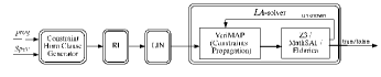
Figure 3: Our software model checker that uses the linearization module LIN.

We performed an experimental evaluation on a set of programs taken from the literature, including some programs from [Felsing et al. (2014)] obtained by applying strength reduction, a real-world optimization technique. In Table 1 we report the results of our experiments.

One can see that linearization takes very little time compared to the total verification time. Moreover, linearization is necessary for the verification of 14 out of 19 programs (including fibonacci), which otherwise cannot be proved correct with respect to their specifications. In the two columns under LA-solving-1 we report the results obtained by giving as input to the Z3 and Eldarica solvers the set PC generated by the RI module. Under LA-solving-1 we do not have a column for MathSAT, because the version of this solver used in our experiments (namely, MSATIC3) cannot deal with nonlinear CHC’s, and therefore it cannot be applied before linearization. In the last three columns of Table 1 we report the results obtained by giving as input to VeriMAP (and the solvers Z3, MatSAT, and Eldarica, respectively) the clauses obtained after linearization.

Unsurprisingly, for the verification problems where linearization is not necessary, our technique may deteriorate the performance, although in most of these problems the solving time does not increase much.

	Program	RI	LA-solving-1		LIN	LA-solving-2: VeriMAP &
			Z3	Eldarica		Z3	MathSAT	Eldarica
1.	binary_division	0.02	4.16	TO	0.04	17.36	17.87	20.98
2.	fast_multiplication_$2$	0.02	TO	3.71	0.01	1.07	1.97	7.59
3.	fast_multiplication_$3$	0.03	TO	4.56	0.02	2.59	2.54	9.31
4.	fibonacci	0.01	TO	TO	0.01	2.00	47.74	6.97
5.	Dijkstra_fusc	0.01	1.02	3.80	0.05	2.14	2.80	10.26
6.	greatest_common_divisor	0.01	TO	TO	0.01	0.89	1.78	0.04
7.	integer_division	0.01	TO	TO	0.01	0.88	1.90	2.86
8.	$91$-function	0.01	1.27	TO	0.06	117.97	14.24	TO
9.	integer_multiplication	0.02	TO	TO	0.01	0.52	14.76	0.54
10.	remainder	0.01	TO	TO	0.01	0.87	1.70	3.16
11.	sum_first_integers	0.01	TO	TO	0.01	1.79	2.30	6.81
12.	lucas	0.01	TO	TO	0.01	2.04	8.39	9.46
13.	padovan	0.01	TO	TO	0.01	2.24	TO	11.62
14.	perrin	0.01	TO	TO	0.02	2.23	TO	11.89
15.	hanoi	0.01	TO	TO	0.01	1.81	2.07	6.59
16.	digits$10$	0.01	TO	TO	0.01	4.52	3.10	6.54
17.	digits$10$-itmd	0.06	TO	TO	0.04	TO	10.26	12.38
18.	digits$10$-opt	0.08	TO	TO	0.10	TO	TO	15.80
19.	digits$10$-opt$100$	0.01	TO	TO	0.02	TO	58.99	8.98

Table 1: Columns RI and LIN show the times $($in seconds$)$ taken for removal of the interpreter and linearization. The two columns under LA-solving-1 show the times taken by Z3 and  Eldarica for solving the problems after RI alone. The three columns under LA-solving-2 show the times taken by VeriMAP together with Z3, MathSAT,  and Eldarica, after RI and LIN. The timeout TO occurs after $120$ seconds.

6 Conclusions and Related Work

We have presented a method for proving partial correctness specifications of programs, given as Hoare triples of the form $\{\varphi\}\,\textit{prog}\,\{\psi\}$, where the assertions $\varphi$ and $\psi$ are predicates defined by a set of possibly recursive, definite CLP clauses. Our verification method is based on: Step (1) a translation of a given specification into a set of constrained Horn clauses (that is, a CLP program together with one or more goals), Step (2) an unfold/fold transformation strategy, called linearization, which derives linear clauses (that is, clauses with at most one atom in their body), and Step (3) an LA-solver that attempts to prove the satisfiability of constrained Horn clauses by interpreting predicates as linear arithmetic constraints.

We have formally proved that the method which uses linearization is strictly more powerful than the method that applies Step (3) immediately after Step (1). We have also developed a proof-of-concept implementation of our method by using the VeriMAP verification system [De Angelis et al. (2014b)] together with various state-of-the-art solvers (namely, Z3 [de Moura and Bjørner (2008)], MathSAT [Cimatti et al. (2013)], and Eldarica [Rümmer et al. (2013)]), and we have shown that our method works on several verification problems. Although these problems refer to quite simple specifications, some of them cannot be solved by using the above mentioned solvers alone.

The use of transformation-based methods in the field of program verification has recently gained popularity (see, for instance, [Albert et al. (2007), De Angelis et al. (2014a), Fioravanti et al. (2013), Kafle and Gallagher (2015), Leuschel and Massart (2000), Lisitsa and Nemytykh (2008), Peralta et al. (1998)]). However, fully automated methods based on various notions of partial deduction and CLP program specialization cannot achieve the same effect as linearization. Indeed, linearization requires the introduction of new predicates corresponding to conjunctions of old predicates, whereas partial deduction and program specialization can only introduce new predicates that correspond to instances of old predicates. In order to derive linear clauses, one could apply conjunctive partial deduction [De Schreye et al. (1999)], which essentially is equivalent to unfold/fold transformation. However, to the best of our knowledge, this application of conjunctive partial deduction to the field of program verification has not been investigated so far.

The use of linear arithmetic constraints for program verification has been first proposed in the field of abstract interpretation [Cousot and Cousot (1977)], where these constraints are used for approximating the set of states that are reachable during program execution [Cousot and Halbwachs (1978)]. In the field of logic programming, abstract interpretation methods work similarly to LA-solving for constrained Horn clauses, because they both look for interpretations of predicates as linear arithmetic constraints that satisfy the program clauses (see, for instance, [Benoy and King (1997)]). Thus, abstract interpretation methods suffer from the same theoretical limitations we have pointed out in this paper for LA-solving methods.

One approach that has been followed for overcoming the limitations related to the use of linear arithmetic constraints is to devise methods for generating polynomial invariants and proving specifications with polynomial arithmetic constraints [Rodríguez-Carbonell and Kapur (2007a), Rodríguez-Carbonell and Kapur (2007b)]. This approach also requires the development of solvers for polynomial constraints, which is a very complex task on its own, as in general the satisfiability of these constraints on the integers is undecidable [Matijasevic (1970)]. In contrast, the approach presented in this paper has the objective of transforming problems which would require the proof of nonlinear arithmetic assertions into problems which can be solved by using linear arithmetic constraints. We have shown some examples (such as the fibonacci program) where we are able to prove specifications whose post-condition is an exponential function.

An interesting issue for future research is to identify general criteria to answer the following question: Given a class $\mathcal{D}$ of constraints and a class $\mathcal{H}$ of constrained Horn clauses, does the satisfiability of a finite set of clauses in $\mathcal{H}$ imply its $\mathcal{D}$-solvability? Theorem 2 provides a negative answer to this question when $\mathcal{D}$ is the class of LA constraints and $\mathcal{H}$ is the class of all constrained Horn clauses.

7 Acknowledgments

We thank the participants in the Workshop VPT ’15 on Verification and Program Transformation, held in London on April 2015, for their comments on a preliminary version of this paper. This work has been partially supported by the National Group of Computing Science (GNCS-INDAM).

Appendix

For the proof of Theorem 1 we need the following lemma.

Lemma 1. (i) The relation $r_{\textit{\small prog}}$ defined by OpSem is a functional relation, that is, $M(\textit{OpSem})\models\forall p_{1},\!\ldots\!,p_{s},y_{1},y_{2}$.$r_{\textit{\small prog}}(p_{1},\!\ldots\!,p_{s},y_{1})\!\wedge\!r_{\textit{\small prog}}(p_{1},\!\ldots\!,p_{s},y_{2})\!\rightarrow\!y_{1}\!\mathchar 61\relax\!y_{2}$.

(ii) A program prog terminates for an environment $\delta_{0}$ such that $\delta_{0}(z_{1})\!\mathchar 61\relax\!p_{1}$,$\ldots$, $\delta_{0}(z_{s})\!\mathchar 61\relax\!p_{s}$ and $\textit{pre}(p_{1},\!\ldots\!,p_{s})$ holds, iff

$M(\textit{OpSem})\models\textit{pre}(p_{1},\!\ldots\!,p_{s})\rightarrow\exists y$. $r_{\textit{\small prog}}(p_{1},\!\ldots\!,p_{s},y)$.

Proof. Since the program prog is deterministic, the predicate $r_{\textit{\small prog}}$ defined by OpSem is a functional relation (which might not be total on pre, as prog might not terminate). Moreover, a program prog, with variables $z_{1},\ldots,z_{s}$, terminates for an environment $\delta_{0}$ such that: (i) $\delta_{0}(z_{1})\!\mathchar 61\relax\!p_{1},$ $\ldots,$ $\delta_{0}(z_{s})\!\mathchar 61\relax\!p_{s}$, and (ii) $\delta_{0}$ satisfies pre, iff $\exists y$. $r_{\textit{\small prog}}(p_{1},\ldots,p_{s},y)$ holds in $M(\textit{OpSem})$.

Proof of Theorem 1 $($Partial Correctness$)$.

Let $\textit{dom}_{r}(X_{1},\ldots,X_{s})$ be a predicate that represents the domain of the functional relation $r_{\textit{prog}}$. We assume that $\textit{dom}_{r}(X_{1},\ldots,X_{s})$ is defined by a set Dom of clauses, using predicate symbols not in $\textit{OpSem}\cup\textit{Spec}$, such that

$M(\textit{OpSem}\cup\textit{Dom})\models$ $(1)$

$\forall X_{1},\ldots,X_{s}\textit{.}((\exists Y\textit{.}r_{\textit{prog}}(X_{1},\ldots,X_{s},Y)\leftrightarrow\textit{dom}_{r}(X_{1},\ldots,X_{s}))$

Let us denote by $\textit{Spec}^{\sharp}$ the set of clauses obtained from Spec by replacing each clause $\textit{f\/}(X_{1},\ldots,X_{s},Y)\leftarrow B$ by the clause $\textit{f\/}(X_{1},\ldots,X_{s},Y)\leftarrow\textit{dom}_{r}(X_{1},\ldots,X_{s}),B$. Then, for all integers $p_{1},\ldots,p_{s},y$,

$M(\textit{Spec}^{\sharp}\cup\textit{Dom})\models\textit{f\/}(p_{1},\ldots,p_{s},y)$  implies  $M(\textit{Spec})\models\textit{f\/}(p_{1},\ldots,p_{s},y)$ (2)

Moreover, let us denote by $\textit{Spec}^{\prime}$ the set of clauses obtained from $\textit{Spec}^{\sharp}$ by replacing all occurrences of $f$ by $r_{\textit{prog}}$. We show that $M(\textit{OpSem}\cup\textit{Aux}\cup\textit{Dom})\models\textit{Spec}^{\prime}$.

Let $S$ be any clause in $\textit{Spec}^{\prime}$. If $S$ belongs to Aux, then $M(\textit{OpSem}\cup\textit{Aux})\models S$. Otherwise, $S$ is of the form $r_{\textit{prog}}(X_{1},\ldots,X_{s},Y)\leftarrow\textit{dom}_{r}(X_{1},\ldots,X_{s}),\widetilde{B}$ and, by construction, in $F_{\textit{pcorr}}$ there are two goals

$G_{1}$: $\textit{false}\leftarrow Y\!\mathchar 62\relax\!Z,r_{\textit{prog}}(X_{1},\ldots,X_{s},Z),\widetilde{B}$, and

$G_{2}$: $\textit{false}\leftarrow Y\!\mathchar 60\relax\!Z,r_{\textit{prog}}(X_{1},\ldots,X_{s},Z),\widetilde{B}$

such that $\textit{OpSem}\cup\textit{Aux}\cup\{G_{1},G_{2}\}$ is satisfiable. Then,

$M(\textit{OpSem}\cup\textit{Aux})\models\neg\exists(Y\neq Z\wedge r_{\textit{prog}}(X_{1},\ldots,X_{s},Z)\wedge\widetilde{B})$

Since $M(\textit{OpSem}\cup\textit{Dom})\models r_{\textit{prog}}(X_{1},\ldots,X_{s},Z)\rightarrow\textit{dom}_{r}(P_{1},\ldots,P_{s})$, we also have that

$M(\!\textit{OpSem}\cup\textit{Aux}\cup\textit{Dom})\!\models\!\neg\exists(\!Y\!\neq\!Z\wedge\textit{dom}_{r}(X_{1},\ldots,X_{s})\wedge r_{\textit{prog}}(X_{1},\ldots,X_{s},Z)\wedge\widetilde{B})$

From the functionality of $r_{\textit{prog}}$ it follows that

$M(\textit{OpSem}\cup\textit{Aux}\cup\textit{Dom})\models\neg r_{\textit{prog}}(X_{1},\ldots,X_{s},Y)$

$\leftrightarrow(\neg\exists Z\mathbin{\cdot}r_{\textit{prog}}(X_{1},\ldots,X_{s},Y)\vee(r_{\textit{prog}}(X_{1},\ldots,X_{s},Z)\wedge Y\!\neq\!Z))$

and hence, by using (1),

$M(\textit{OpSem}\cup\textit{Aux}\cup\textit{Dom})\models\neg\exists(\textit{dom}_{r}(X_{1},\ldots,X_{s})\wedge\neg r_{\textit{prog}}(X_{1},\ldots,X_{s},Y)\wedge\widetilde{B})$

Thus, we have that

$M(\textit{OpSem}\cup\textit{Aux}\cup\textit{Dom})\models\forall(\textit{dom}_{r}(X_{1},\ldots,X_{s})\wedge\widetilde{B}\rightarrow r_{\textit{prog}}(X_{1},\ldots,X_{s},Y))$

that is, clause $S$ is true in $M(\textit{OpSem}\cup\textit{Aux}\cup\textit{Dom})$. We can conclude that $M(\textit{OpSem}\cup\textit{Aux}\cup\textit{Dom})$ is a model of $\textit{Spec}^{\prime}\cup\textit{Dom}$, and since $M(\textit{Spec}^{\prime}\cup\textit{Dom})$ is the least model of $\textit{Spec}^{\prime}\cup\textit{Dom}$, we have that

$M(\textit{Spec}^{\prime}\cup\textit{Dom})\subseteq M(\textit{OpSem}\cup\textit{Aux}\cup\textit{Dom})$ (3)

Next we show that, for all integers $p_{1},\ldots,p_{s},y$,

$M(\textit{Spec}^{\sharp}\cup\textit{Dom})\models f(p_{1},\ldots,p_{s},y)$   iff   $M(\textit{OpSem})\models r_{\textit{prog}}(p_{1},\ldots,p_{s},y)$ (4)

Only If Part of (4). Suppose that $M(\textit{Spec}^{\sharp}\cup\textit{Dom})\models f(p_{1},\ldots,p_{s},y)$. Then, by construction,

$M(\textit{Spec}^{\prime}\cup\textit{Dom})\models r_{\textit{prog}}(p_{1},\ldots,p_{s},y)$

and hence, by (3),

$M(\textit{OpSem}\cup\textit{Aux}\cup\textit{Dom})\models r_{\textit{prog}}(p_{1},\ldots,p_{s},y)$

Since $r_{\textit{prog}}$ does not depend on predicates in $\textit{Aux}\cup\textit{Dom}$,

$M(\textit{OpSem})\models r_{\textit{prog}}(p_{1},\ldots,p_{s},y)$

If Part of (4). Suppose that $M(\textit{OpSem})\models r_{\textit{prog}}(p_{1},\ldots,p_{s},y)$.

Then, by definition of $r_{\textit{prog}}$,

$M(\textit{Dom})\models{\textit{dom}_{r}}(p_{1},\ldots,p_{s})$ (5)

and

$M(\textit{Spec})\models{\textit{pre}}(p_{1},\ldots,p_{s})$ (6)

Thus, by (6) and Condition (3.1) of Definition 1, there exists $z$ such that

$M(\textit{Spec})\models f(p_{1},\ldots,p_{s},z)$ (7)

By (5) and (7),

$M(\textit{Spec}^{\sharp}\cup\textit{Dom})\models f(p_{1},\ldots,p_{s},z)$ (8)

By the Only If Part of (4),

$M(\textit{OpSem})\models r_{\textit{prog}}(p_{1},\ldots,p_{s},z)$

and by the functionality of $r_{\textit{prog}}$, $z\mathchar 61\relax y$. Hence, by (8),

$M(\textit{Spec}^{\sharp}\cup\textit{Dom})\models f(p_{1},\ldots,p_{s},y)$

Let us now prove partial correctness. If $M(\textit{Spec})\models{\textit{pre}}(p_{1},\ldots,p_{s})$ and prog terminates, that is, $M(\textit{Dom})\models\textit{dom}_{r}(p_{1},\ldots,p_{s})$, then for some integer $y$, $M(\textit{OpSem})\models r_{\textit{prog}}(p_{1},\ldots,p_{s},y)$. Thus, by (4), $M(\textit{Spec}^{\sharp}\cup\textit{Dom})\models f(p_{1},\ldots,p_{s},y)$ and hence, by (2), $M(\textit{Spec})\models f(p_{1},\ldots,p_{s},y)$. Suppose that the postcondition $\psi$ is $f(p_{1},\ldots,p_{s},z_{k})$. Then, by Condition (3.2) of Definition 1, $y\mathchar 61\relax z_{k}$.

Thus, $\{\varphi\}$ prog $\{\psi\}$.

Removal of the Interpreter

Here we report the variant of the transformation presented in [De Angelis et al. (2014a)] that we use in this paper to perform the removal of the interpreter. In this transformation we use the function $\textit{Unf\/}(C,A,{\mathit{C}ls})$ defined as the set of clauses derived by unfolding a clause $C$ with respect to an atom $A$ using the set Cls of clauses (see the unfolding rule in Section 4.2).

The predicate reach is defined as follows:

${\mathit{r}each}(X,X)\leftarrow$

${\mathit{r}each}(X,Z)\leftarrow{\mathit{t}r}(X,Y),\ {\mathit{r}each}(Y,Z)$

where, as mentioned in Section 2, tr is a (nonrecursive) predicate representing one transition step according to the operational semantics of the imperative language.

In order to perform the Unfolding step, we assume that the atoms occurring in bodies of clauses are annotated as either unfoldable or not unfoldable. This annotation ensures that any sequence of clauses constructed by unfolding w.r.t. unfoldable atoms is finite. In particular, the atoms with predicate initCf, finalCf, and tr are unfoldable. The atoms of the form $\textit{reach}(\textit{cf}_{1},\textit{cf}_{2})$ are unfoldable if $\textit{cf}_{1}$ is not associated with a while or goto command. Other annotations based on a different analysis of program ${\mathit{O}pSem}$ can be used.

Input: Program OpSem.
Output: Program $\textit{OpSem}_{\textit{\small{RI}}}$ such that, for all integers $p_{1},\ldots,\!p_{s},\!z_{k}$,

$r_{\textit{\small prog}}(\!p_{1},\ldots,\!p_{s},\!z_{k})\!\in\!M(\textit{OpSem})$ iff $r_{\textit{\small prog}}(\!p_{1},\ldots,\!p_{s},\!z_{k})\!\in\!M(\textit{OpSem}_{\textit{\small{RI}}})$.
 

Initialization:

$\textit{OpSem}_{\textit{\small{RI}}}:\mathchar 61\relax\emptyset$;   $\textit{Defs}:\mathchar 61\relax\emptyset$;

$\textit{InCls}:\mathchar 61\relax\!\{r_{\textit{\small prog}}(\!P_{1},\!\ldots\!,\!P_{s},\!Z_{k}\!)\!\leftarrow\!\textit{initCf\/}(\!C_{0},\!P_{1},\!\ldots\!,\!P_{s}),\textit{reach}(\!C_{0},\!\textit{C}_{h}),\textit{finalCf\/}(\!C_{h},\!Z_{k})\!\}$;

while in InCls there is a clause $C$ which is not a constrained fact do

Unfolding:

$\textit{SpC}:\mathchar 61\relax\textit{Unf}(C,A,\textit{OpSem})$, where A is the leftmost atom in the body of $C$;

while in SpC there is a clause $D$ whose body contains an occurrence of an unfoldable atom A do
$\textit{\leavevmode\nobreak\ \leavevmode\nobreak\ \leavevmode\nobreak\ SpC}:\mathchar 61\relax(\textit{SpC}\mathchar 45\relax\{D\})\cup\ \textit{Unf}(D,A,\textit{OpSem})$

end-while;

Definition & Folding:

while in SpC there is a clause $E$ of the form:   $H\leftarrow e,\textit{reach}(\textit{cf}_{1},\textit{cf}_{2})$

do

ifin Defs there is no clause of the form:   $\textit{newp}(V)\leftarrow\textit{reach}(\textit{cf}_{1},\textit{cf}_{2})$

where V is the set of variables occurring in $\textit{reach}(\textit{cf}_{1},\textit{cf}_{2})$

then  add the clause $N$: $\textit{newp}(V)\leftarrow\textit{reach}(\textit{cf}_{1},\textit{cf}_{2})$ to Defs and InCls;

$\textit{SpC}:\mathchar 61\relax(\textit{SpC}\mathchar 45\relax\{E\})\cup\{H\leftarrow e,\textit{newp}(V)\}$

end-while;

$\textit{InCls}:\mathchar 61\relax\textit{InCls}\mathchar 45\relax\{C\}$;    $\textit{OpSem}_{\textit{\small{RI}}}:\mathchar 61\relax\textit{OpSem}_{\textit{\small{RI}}}\cup\textit{SpC}$;

end-while;

RI: Removal of the Interpreter.

Let us now prove Theorem 3 stating the relevant properties of the RI transformation.

The RI transformation terminates. The termination of the Unfolding step is guaranteed by the unfoldable annotations. Indeed, (i) the repeated unfolding of the unfoldable atoms with predicates initCf, finalCf, and tr, always terminates because those atoms have no recursive clauses, (ii) by the definition of the semantics of the imperative program, the repeated unfolding of an atom of the form $\textit{reach}(\textit{cf}_{1},\textit{cf}_{2})$ eventually derives a new $\textit{reach}(\textit{cf}_{3},\textit{cf}_{4})$ atom where $\textit{cf}_{3}$ is either a final configuration or a configuration associated with a while or goto command, and in both cases unfolding terminates. The termination of the Definition & Folding step follows from the fact that SpC is a finite set of clauses.

The outer while loop terminates because a finite set of new predicate definitions of the form $\textit{newp}(V)\leftarrow\textit{reach}(\textit{cf}_{1},\textit{cf}_{2})$ can be introduced. Indeed, each configuration cf is represented as a term cf(LC,E)), where LC is a labeled command and E is an environment (see Example 1). An environment is represented as a list of $(v,X)$ pairs where $v$ is a variable identifier and $X$ is its value, that is, a logical variable whose value may be subject to a given constraint. Considering that: (i) the labeled commands and the variable identifiers occurring in an imperative program are finitely many, and (ii) predicate definitions of the form $\textit{newp}(V)\leftarrow\textit{reach}(\textit{cf}_{1},\textit{cf}_{2})$ abstract away from the constraints that hold on the logical variables occurring in $\textit{cf}_{1}$ and $\textit{cf}_{2}$, we can conclude that there are only finitely many such clauses (modulo variable renaming).

Point 1: $\textit{OpSem}_{\textit{\small{RI}}}$ is a set of linear clauses over the integers. By construction, every clause in $\textit{OpSem}_{\textit{\small{RI}}}$ is of the form $H\leftarrow c,B$, where (i) $H$ is either $r_{\textit{\small prog}}(\!P_{1},\ldots,\!P_{s},\!Z_{k})$ or $\textit{newp}(V)$, for some new predicate newp and tuple of variables $V$, and (ii) $B$ is either absent or of the form $\textit{newp}(V)$, for some new predicate newp and tuple of variables $V$. Thus, every clause is a linear clause over the integers.

Point 2: $\textit{OpSem}\cup\textit{Aux}\,\cup F_{\textit{\small{pcorr}}}$ is satisfiable iff $\textit{OpSem}_{\textit{\small{RI}}}\cup\textit{Aux}\,\cup F_{\textit{\small{pcorr}}}$ is satisfiable. From the correctness of the unfolding, definition, and folding rules with respect to the least model semantics of CLP programs [Etalle and Gabbrielli (1996)], it follows that, for all integers $p_{1},\ldots,\!p_{s},\!z_{k}$,

$r_{\textit{\small prog}}(p_{1},\ldots,\!p_{s},\!z_{k})\!\in\!M(\textit{OpSem})$ iff $r_{\textit{\small prog}}(p_{1},\ldots,\!p_{s},\!z_{k})\!\in\!M(\textit{OpSem}_{\textit{\small{RI}}})$ $(\dagger 1)$

$\textit{OpSem}\cup\textit{Aux}\,\cup F_{\textit{\small{pcorr}}}$ is satisfiable iff for every ground instance $G$ of a goal in $F_{\textit{\small{pcorr}}}$, $M(\textit{OpSem}\cup\textit{Aux})\models G$. Since the only predicate of OpSem on which $G$ may depend is $r_{\textit{\small prog}}$, by $(\dagger 1)$, we have that $M(\textit{OpSem}\cup\textit{Aux})\models G$ iff $M(\textit{OpSem}_{\textit{\small{RI}}}\cup\textit{Aux})\models G$. Finally, $M(\textit{OpSem}_{\textit{\small{RI}}}\cup\textit{Aux})\models G$ for every ground instance $G$ of a goal in $F_{\textit{\small{pcorr}}}$, iff $\textit{OpSem}_{\textit{\small{RI}}}\cup\textit{Aux}\,\cup F_{\textit{\small{pcorr}}}$ is satisfiable.

Point 3: $\textit{OpSem}\,\cup\textit{Aux}\,\cup F_{\textit{\small{pcorr}}}$ is LA-solvable iff $\textit{OpSem}_{\textit{\small{RI}}}\,\cup\textit{Aux}\,\cup F_{\textit{\small{pcorr}}}$ is LA-solvable.

Suppose that $\textit{OpSem}\,\cup\textit{Aux}\,\cup F_{\textit{\small{pcorr}}}$ is LA-solvable, and let $\Sigma$ be an LA-solution of $\textit{OpSem}\,\cup\textit{Aux}\,\cup F_{\textit{\small{pcorr}}}$. Now we construct an LA-solution $\Sigma_{\textit{\small{RI}}}$ of $\textit{OpSem}_{\textit{\small{RI}}}\,\cup\textit{Aux}\,\cup F_{\textit{\small{pcorr}}}$. To this purpose it is enough to define a symbolic interpretation for the new predicates introduced by RI.

For any predicate newp introduced by RI via a clause of the form:

$\textit{newp}(V)\leftarrow\textit{reach}(\textit{cf}_{1},\textit{cf}_{2})$

we define a symbolic interpretation as follows:

$\Sigma_{\textit{\small{RI}}}(\textit{newp}(V))\mathchar 61\relax\Sigma(\textit{reach}(\textit{cf}_{1},\textit{cf}_{2}))$

Moreover, $\Sigma_{\textit{\small{RI}}}$ is identical to $\Sigma$ for the atoms with predicate occurring in OpSem.

Now we have to prove that $\Sigma_{\textit{\small{RI}}}$ is indeed an LA-solution of $\textit{OpSem}_{\textit{\small{RI}}}\,\cup\textit{Aux}\,\cup F_{\textit{\small{pcorr}}}$. This proof is similar to the proof of Theorem 5 (actually, simpler, because RI introduces new predicates defined by single atoms, while LIN introduces new predicates defined by conjunctions of atoms), and is omitted.

Vice versa, if $\Sigma_{\textit{\small{RI}}}$ is an LA-solution of $\textit{OpSem}_{\textit{\small{RI}}}\,\cup\textit{Aux}\,\cup F_{\textit{\small{pcorr}}}$, we construct an LA-solution $\Sigma$ of $\textit{OpSem}\,\cup\textit{Aux}\,\cup F_{\textit{\small{pcorr}}}$ by defining

$\Sigma(\textit{reach}(\textit{cf}_{1},\textit{cf}_{2}))\mathchar 61\relax\Sigma_{\textit{\small{RI}}}(\textit{newp}(V))$.

Proof of Theorem 4

Let LCls be a set of linear clauses and Gls be a set of nonlinear goals. We split the proof of Theorem 4 in three parts:

Termination: The linearization transformation LIN terminates for the input set of clauses $\textit{LCls}\,\cup\textit{Gls}$;

Linearity: The output TransfCls of LIN is a set of linear clauses;

Equisatisfiability: $\textit{LCls}\,\cup\textit{Gls}$ is satisfiable iff TransfCls is satisfiable.

(Termination) Each Unfolding and Definition & Folding step terminates. Thus, in order to prove the termination of LIN it is enough to show that the while loop is executed a finite number of times, that is, a finite number of clauses are added to NLCls. We will establish this finiteness property by showing that there exists an integer $M$ such that every clause added to NLCls is of the form:

$\textit{newp}(X_{1},\ldots,X_{t})\leftarrow A_{1},\ldots,A_{k}$ $(\dagger 2)$

where: (i) $k\leq M$, (ii) for $i\mathchar 61\relax 1,\ldots,k$, $A_{i}$ is of the form $p(X_{1},\ldots,X_{m})$, and (iii) $\{X_{1},\ldots,X_{t}\}\subseteq\textit{vars}(A_{1},\ldots,A_{k})$.

Indeed, let $M$ be the maximal number of atoms occurring in the body of a goal in Gls, to which NLCls is initialized. Now let us consider a clause $C$ in NLCls and assume that in the body of $C$ there are at most $M$ atoms. The clauses in the set LCls used for unfolding $C$ are linear, and hence in the body of each clause belonging to the set $U(C)$ obtained after the Unfolding step, there are at most $M$ atoms. Thus, each clause in $U(C)$ is of the form $H\leftarrow c,A_{1},\ldots,A_{k}$, with $k\leq M$. Since the body of every new clause introduced by the subsequent Definition & Folding step is obtained by dropping the constraint from the body of a clause in $U(C)$, we have that every clause added to NLCls is of the form $(\dagger 2)$, with $k\leq M$. Thus, LIN terminates.

(Linearity) TransfCls is initialized to the set LCls of linear clauses. Moreover, each clause added to TransfCls is of the form $H\leftarrow c,\,\textit{newp}(X_{1},\ldots,X_{t})$, and hence is linear.

(Equisatisfiability) In order to prove that LIN ensures equisatisfiability, let us adapt to our context the basic notions about the unfold/fold transformation rules for CLP programs presented in [Etalle and Gabbrielli (1996)].

Besides the unfolding rule of Section 4.2, we also introduce the following definition and folding rules.

Definition Rule. By definition we introduce a clause of the form $\textit{newp}(X)\leftarrow G$, where newp is a new predicate symbol and $X$ is a tuple of variables occurring in G.

Folding Rule. Given a clause $E$: ${H\leftarrow c,G}$ and a clause $D$: ${\textit{newp}(X)\leftarrow G}$ introduced by the definition rule. Suppose that, ${\textit{X}}\mathchar 61\relax\textit{vars}({\mathit{G}})\cap\textit{vars}(\textit{H,c})$. Then by folding $E$ using $D$ we derive $H\leftarrow c,\textit{newp}(X)$.

From a set Cls of clauses we can derive a new set TransfCls of clauses either by adding a new clause to Cls using the definition rule or by: (i) selecting a clause $C$ in Cls, (ii) deriving a new set TransfC of clauses using one or more transformation rules among unfolding and folding, and (iii) replacing $C$ by TransfC in Cls. We can apply a new sequence of transformation rules starting from TransfCls and iterate this process at will.

The following theorem is an immediate consequence of the correctness results for the unfold/fold transformation rules of CLP programs [Etalle and Gabbrielli (1996)].

Theorem 6 (Correctness of the Transformation Rules)

Let the set TransfCls be derived from Cls by a sequence of applications of the unfolding, definition and folding transformation rules. Suppose that every clause introduced by the definition rule is unfolded at least once in this sequence. Then, Cls is satisfiable iff TransfCls is satisfiable.

Now, equisatisfiability easily follows from Theorem 6. Indeed, the Unfolding and Definition & Folding steps of LIN are applications of the unfolding, definition, and folding rules (strictly speaking, the rewriting performed after unfolding is not included among the transformation rules, but obviously preserves all LA-models). Moreover, every clause introduced during the Definition & Folding step is added to NCls and unfolded in a subsequent step of the transformation. Thus, the hypotheses of Theorem 6 are fulfilled, and hence we have that $\textit{LCls}\,\cup\textit{Gls}$ is satisfiable iff TransfCls is satisfiable.

Linearized clauses for Fibonacci.

The set of linear constrained Horn clauses obtained after applying LIN is made out of clauses E1, E2, E3, and C3, together with the following clauses:

new1(N1,U,V,U,N2,U,N3,U):- N1=<0, N2=<0, N3=<0.

new1(N1,U,V,U,N2,U,N3,F3):- N1=<0, N2=<0, N4=N3-1, W=U+V, N3>=1,new2(N4,W,U,F3).

new1(N1,U,V,U,N2,F2,N3,U):- N1=<0, N4=N2-1, W=U+V, N2>=1, N3=<0,new2(N4,W,U,F2).

new1(N1,U,V,U,N2,F2,N3,F3):- N1=<0, N4=N2-1, N2>=1, N5=N3-1, N3>=1,

new3(N4,W,U,F2,N5,F3).

new1(N1,U,V,F1,N2,U,N3,U):- N4=N1-1, W=U+V, N1>=1, N2=<0, N3=<0,new2(N4,W,U,F1).

new1(N1,U,V,F1,N2,U,N3,F3):- N4=N1-1, N1>=1, N2=<0, N5=N3-1, W=U+V, N3>=1,

new3(N4,W,U,F1,N5,F3).

new1(N1,U,V,F1,N2,F2,N3,U):- N4=N1-1, N1>=1, N5=N2-1, W=U+V, N2>=1, N3=<0,

new3(N4,W,U,F1,N5,F2).

new1(N1,U,V,F1,N2,F2,N3,F3):- N4=N1-1, N1>=1, N5=N2-1, N2>=1, N6=N3-1, W=U+V,

N3>=1, new1(N4,W,U,F1,N5,F2,N6,F3).

new2(N,U,V,U):- N=<0.

new2(N,U,V,F):- N2=N-1, W=U+V, N>=1, new2(N2,W,U,F).

new3(N1,U,V,U,N2,U):- N1=<0, N2=<0.

new3(N1,U,V,U,N2,F2):- N1=<0, N3=N2-1, W=U+V, N2>=1, new2(N3,W,U,F2).

new3(N1,U,V,F1,N2,F2):- N3=N1-1, N1>=1, N4=N2-1, W=U+V, N2>=1,

new3(N3,W,U,F1,N4,F2).

new3(N1,U,V,F1,N2,U):- N3=N1-1, W=U+V, N1>=1, N2=<0, new2(N3,W,U,F1).

Proof of Theorem 5 $($Monotonicity with respect to LA-Solvability$)$.

Suppose that the set $\textit{LCls}\cup\textit{Gls}$ of constrained Horn clauses is LA-solvable, and let TransfCls be obtained by applying LIN to $\textit{LCls}\cup\textit{Gls}$. Let $\Sigma$ be an LA-solution of $\textit{LCls}\cup\textit{Gls}$. We now construct an LA-solution of TransfCls. For any predicate newp introduced by LIN via a clause of the form:

$\textit{newp}(X_{1},\ldots,X_{t})\leftarrow A_{1},\ldots,A_{k}$

we define a symbolic interpretation $\Sigma^{\prime}$ as follows:

$\Sigma^{\prime}(\textit{newp}(X_{1},\ldots,X_{t}))\mathchar 61\relax\Sigma(A_{1})\wedge\ldots\wedge\Sigma(A_{k})$

Now, we are left with the task of proving that $\Sigma^{\prime}$ is indeed an LA-solution of TransfCls. The clauses in TransfCls are either of the form

$\textit{false}\leftarrow c,\textit{newq}(X_{1},\ldots,X_{u})$

or of the form

$\textit{newp}(X_{1},\ldots,X_{t})\leftarrow c,\textit{newq}(X_{1},\ldots,X_{u})$

where newp and newq are predicates introduced by LIN. We will only consider the more difficult case where the conclusion is not false.

The clause $\textit{newp}(X_{1},\ldots,X_{t})\leftarrow c,\textit{newq}(X_{1},\ldots,X_{u})$ has been derived (see the linearization transformation LIN in Figure 2) in the following two steps.

(Step i) Unfolding $\textit{newp}(X_{1},\ldots,X_{t})\leftarrow A_{1},\ldots,A_{k}$ w.r.t. all atoms in its body using $k$ clauses in LCls:

$A_{1}\leftarrow c_{1},B_{1}\ \ \ldots\ \ A_{k}\leftarrow c_{k},B_{k}$

where some of the $B_{i}$’s can be the true and $c\equiv c_{1},\ldots,c_{k}$, thereby deriving

$\textit{newp}(X_{1},\ldots,X_{t})\leftarrow c_{1},\ldots,c_{k},B_{1},\ldots,B_{k}$

(Without loss of generality we assume that the atoms in the body of the clauses are equal to, instead of unifiable with, the heads of the clauses in LCls. )

(Step ii) Folding $\textit{newp}(X_{1},\ldots,X_{t})\leftarrow c_{1},\ldots,c_{k},B_{1},\ldots,B_{k}$ using a clause of the form:

$\textit{newq}(X_{1},\ldots,X_{u})\leftarrow B_{1},\ldots,B_{k}$

Thus, for $\textit{newq}(X_{1},\ldots,X_{u}))$ we have the following symbolic interpretation:

$\Sigma^{\prime}(\textit{newq}(X_{1},\ldots,X_{u}))\mathchar 61\relax\Sigma(B_{1})\wedge\ldots\wedge\Sigma(B_{k})$

To prove that $\Sigma^{\prime}$ is an LA-solution of TransfCls, we have to show that

$\textit{LA}\models\forall(c\wedge\Sigma^{\prime}(\textit{newq}(X_{1},\ldots,X_{u}))\rightarrow\Sigma^{\prime}(\textit{newp}(X_{1},\ldots,X_{t})))$

Assume that

$\textit{LA}\models c\wedge\Sigma^{\prime}(\textit{newq}(X_{1},\ldots,X_{u}))$

Then, by definition of $\Sigma^{\prime}$,

$\textit{LA}\models c\wedge\Sigma(B_{1})\wedge\ldots\wedge\Sigma(B_{k})$

Since $\Sigma$ is an LA-solution of LCls, we have that:

${\mathit{L}A}\models\forall(c_{1}\wedge\Sigma(B_{1})\rightarrow\Sigma(A_{1}))\ \ \ldots\ \ \textit{LA}\models\forall(c_{k}\wedge\Sigma(B_{k})\rightarrow\Sigma(A_{k}))$

and hence

$\textit{LA}\models\Sigma(A_{1})\wedge\ldots\wedge\Sigma(A_{k})$

Thus, by definition of $\Sigma^{\prime}$,

$\textit{LA}\models\Sigma^{\prime}(\textit{newp}(X_{1},\ldots,X_{t}))\mathbin{\cdot}$

References

- Albert et al. (2007) Albert, E., Gómez-Zamalloa, M., Hubert, L., and Puebla, G. 2007. Verification of Java Bytecode Using Analysis and Transformation of Logic Programs. In Practical Aspects of Declarative Languages, M. Hanus, Ed. Lecture Notes in Computer Science 4354. Springer, 124–139.
- Apt et al. (2009) Apt, K. R., de Boer, F. S., and Olderog, E.-R. 2009. Verification of Sequential and Concurrent Programs, Third ed. Springer.
- Benoy and King (1997) Benoy, F. and King, A. 1997. Inferring argument size relationships with CLP(R). In Proceedings of the 6th International Workshop on Logic Program Synthesis and Transformation, LOPSTR ’96, Stockholm, Sweden, August 28-30, 1996, J. P. Gallagher, Ed. Lecture Notes in Computer Science 1207. Springer, 204–223.
- Bjørner et al. (2012) Bjørner, N., McMillan, K., and Rybalchenko, A. 2012. Program verification as satisfiability modulo theories. In Proceedings of the 10th International Workshop on Satisfiability Modulo Theories, SMT-COMP ’12. 3–11.
- Cimatti et al. (2013) Cimatti, A., Griggio, A., Schaafsma, B., and Sebastiani, R. 2013. The MathSAT5 SMT Solver. In Proceedings of TACAS, N. Piterman and S. Smolka, Eds. Lecture Notes in Computer Science 7795. Springer.
- Cousot and Cousot (1977) Cousot, P. and Cousot, R. 1977. Abstract interpretation: A unified lattice model for static analysis of programs by construction of approximation of fixpoints. In Proceedings of the 4th ACM-SIGPLAN Symposium on Principles of Programming Languages, POPL ’77. ACM, 238–252.
- Cousot and Halbwachs (1978) Cousot, P. and Halbwachs, N. 1978. Automatic discovery of linear restraints among variables of a program. In Proceedings of the Fifth ACM Symposium on Principles of Programming Languages, POPL ’78. ACM, 84–96.
- De Angelis et al. (2014a) De Angelis, E., Fioravanti, F., Pettorossi, A., and Proietti, M. 2014a. Program verification via iterated specialization. Science of Computer Programming 95, Part 2, 149–175. Selected and extended papers from Partial Evaluation and Program Manipulation 2013.
- De Angelis et al. (2014b) De Angelis, E., Fioravanti, F., Pettorossi, A., and Proietti, M. 2014b. VeriMAP: A Tool for Verifying Programs through Transformations. In Proceedings of the 20th International Conference on Tools and Algorithms for the Construction and Analysis of Systems, TACAS ’14. Lecture Notes in Computer Science 8413. Springer, 568–574. Available at: http://www.map.uniroma2.it/VeriMAP.
- de Moura and Bjørner (2008) de Moura, L. M. and Bjørner, N. 2008. Z3: An efficient SMT solver. In Proceedings of the 14th International Conference on Tools and Algorithms for the Construction and Analysis of Systems, TACAS ’08. Lecture Notes in Computer Science 4963. Springer, 337–340.
- De Schreye et al. (1999) De Schreye, D., Glück, R., Jørgensen, J., Leuschel, M., Martens, B., and Sørensen, M. H. 1999. Conjunctive Partial Deduction: Foundations, Control, Algorithms, and Experiments. Journal of Logic Programming 41, 2–3, 231–277.
- Etalle and Gabbrielli (1996) Etalle, S. and Gabbrielli, M. 1996. Transformations of CLP modules. Theoretical Computer Science 166, 101–146.
- Felsing et al. (2014) Felsing, D., Grebing, S., Klebanov, V., Rümmer, P., and Ulbrich, M. 2014. Automating Regression Verification. In Proceedings of the 29th ACM/IEEE International Conference on Automated Software Engineering, ASE ’14. ACM, 349–360.
- Fioravanti et al. (2013) Fioravanti, F., Pettorossi, A., Proietti, M., and Senni, V. 2013. Generalization strategies for the verification of infinite state systems. Theory and Practice of Logic Programming. Special Issue on the 25th Annual GULP Conference 13, 2, 175–199.
- Grebenshchikov et al. (2012) Grebenshchikov, S., Lopes, N. P., Popeea, C., and Rybalchenko, A. 2012. Synthesizing software verifiers from proof rules. In Proceedings of the ACM SIGPLAN Conference on Programming Language Design and Implementation, PLDI ’12. 405–416.
- Hoare (1969) Hoare, C. 1969. An Axiomatic Basis for Computer Programming. CACM 12, 10 (October), 576–580, 583.
- Jaffar and Maher (1994) Jaffar, J. and Maher, M. 1994. Constraint logic programming: A survey. Journal of Logic Programming 19/20, 503–581.
- Jaffar et al. (2012) Jaffar, J., Murali, V., Navas, J. A., and Santosa, A. E. 2012. TRACER: A Symbolic Execution Tool for Verification. In Proceedings 24th International Conference on Computer Aided Verification, CAV ’12. Lecture Notes in Computer Science 7358. Springer, 758–766. http://paella.d1.comp.nus.edu.sg/tracer/.
- Kafle and Gallagher (2015) Kafle, B. and Gallagher, J. P. 2015. Constraint Specialisation in Horn Clause Verification. In Proceedings of the 2015 Workshop on Partial Evaluation and Program Manipulation, PEPM ’15, Mumbai, India, January 15–17, 2015. ACM, 85–90.
- Lloyd (1987) Lloyd, J. W. 1987. Foundations of Logic Programming. Springer, Berlin. 2nd Edition.
- Leuschel and Massart (2000) Leuschel, M. and Massart, T. 2000. Infinite state model checking by abstract interpretation and program specialization. In Proceedings of the 9th International Workshop on Logic-based Program Synthesis and Transformation (LOPSTR ’99), Venezia, Italy, A. Bossi, Ed. Lecture Notes in Computer Science 1817. Springer, 63–82.
- Lisitsa and Nemytykh (2008) Lisitsa, A. and Nemytykh, A. P. 2008. Reachability analysis in verification via supercompilation. Int. J. Found. Comput. Sci. 19, 4, 953–969.
- Matijasevic (1970) Matijasevic, Y. V. 1970. Enumerable sets are diophantine. Doklady Akademii Nauk SSSR (in Russian) 191, 279–282.
- Peralta et al. (1998) Peralta, J. C., Gallagher, J. P., and Saglam, H. 1998. Analysis of Imperative Programs through Analysis of Constraint Logic Programs. In Proceedings of the 5th International Symposium on Static Analysis, SAS ’98, G. Levi, Ed. Lecture Notes in Computer Science 1503. Springer, 246–261.
- Podelski and Rybalchenko (2007) Podelski, A. and Rybalchenko, A. 2007. ARMC: The Logical Choice for Software Model Checking with Abstraction Refinement. In Practical Aspects of Declarative Languages, PADL ’07, M. Hanus, Ed. Lecture Notes in Computer Science 4354. Springer, 245–259.
- Reynolds (1998) Reynolds, C. J. 1998. Theories of Programming Languages. Cambridge University Press.
- Rodríguez-Carbonell and Kapur (2007a) Rodríguez-Carbonell, E. and Kapur, D. 2007a. Automatic generation of polynomial invariants of bounded degree using abstract interpretation. Sci. Comput. Program. 64, 1, 54–75.
- Rodríguez-Carbonell and Kapur (2007b) Rodríguez-Carbonell, E. and Kapur, D. 2007b. Generating all polynomial invariants in simple loops. J. Symb. Comput. 42, 4, 443–476.
- Rümmer et al. (2013) Rümmer, P., Hojjat, H., and Kuncak, V. 2013. Disjunctive interpolants for Horn-clause verification. In Proceedings of the 25th International Conference on Computer Aided Verification, CAV ’13, Saint Petersburg, Russia, July 13–19, 2013, N. Sharygina and H. Veith, Eds. Lecture Notes in Computer Science 8044. Springer, 347–363.
- Sebelik and Stepánek (1982) Sebelik, J. and Stepánek, P. 1982. Horn clause programs for recursive functions. In Logic Programming, K. L. Clark and S.-A. Tärnlund, Eds. Academic Press, 325–340.