Entanglement Entropy for Singular Surfaces in Hyperscaling violating Theories

Mohsen Alishahiha^a, Amin Faraji Astaneh^b, Piermarco Fonda^c and Farzad Omidi^d

^a School of Physics, ^b School of Particles and Accelerators, ^d School of Astronomy,
Institute for Research in Fundamental Sciences (IPM)
P.O. Box 19395-5531, Tehran, Iran
^c SISSA and INFN, via Bonomea 265, 34136, Trieste, Italy
E-mails: alishah@ipm.ir, faraji@ipm.ir, piermarco.fonda@sissa.it,
farzad@ipm.ir

We study the holographic entanglement entropy for singular surfaces in theories described holographically by hyperscaling violating backgrounds. We consider singular surfaces consisting of cones or creases in diverse dimensions. The structure of UV divergences of entanglement entropy exhibits new logarithmic terms whose coefficients, being cut-off independent, could be used to define new central charges in the nearly smooth limit. We also show that there is a relation between these central charges and the one appearing in the two-point function of the energy-momentum tensor. Finally we examine how this relation is affected by considering higher-curvature terms in the gravitational action.

1 Introduction

It is well known that the central charge of a two dimensional conformal field theory is an important quantity characterizing its behaviour: it is ubiquitous in many expressions such as the central extension of Virasoro algebra, the two point function of energy-momentum tensor, in the Weyl anomaly and is the coefficient of the logarithmically divergent term in the entanglement entropy [1]. It also appears in the expression of Cardy’s formula for the entropy. Actually the corresponding central charge may be thought of as a measure of the number of degrees of freedom of the theory. Moreover Zamolodchikov’s c-theorem in two dimensions indicates that in any renormalization group flow connecting two fixed points, the central charge decreases along the flow, thus indicating that IR fixed points are characterized by fewer degrees of freedom.

In higher dimensional conformal field theories the situation is completely different. First of all the conformal group in higher dimensions does not have a central extension and thus it is finite dimensional. Moreover the parameter which appears in the two point function of the energy-momentum tensor is not generally related to the one multiplying the Euler density in the Weyl anomaly in even dimensional conformal field theories, nor is directly related to the cut-off independent terms of the entanglement entropy computed for a smooth entangling region.

Indeed if one computes entanglement entropy for a given smooth entangling region in a $d+1$ dimensional conformal field theory, one finds [4, 5]

$$S_{E}=\sum_{i=0}^{[\frac{d}{2}]-1}\frac{A_{2i}}{d-2i-1}\;\frac{1}{\varepsilon^{d-2i-1}}+{\delta_{2[\frac{d}{2}]+1,d}}\;{A_{2[\frac{d}{2}]}}\log\frac{H}{\varepsilon}+{\rm finite\;terms},$$ (1.1)

where $\varepsilon$ is a UV cut off, $A_{i}$’s are some constant parameters (in particular $A_{0}$ is proportional to the area of the enclosed entangling region) and $[x]$ denotes the integer part of $x$. $H$ is a typical scale in the model which could be the size of entangling region. For an even dimensional field theory (odd $d$ in our notation) the coefficient of the logarithmic term, $A_{2[\frac{d}{2}]}$, is a universal constant in the sense that it is independent of the UV cut off: in other words it is fixed by the intrinsic properties of the theory. Two dimensional CFTs fall in this case since the central charge is indeed a universal quantity.

In general for an even dimensional conformal field theory it can be shown that the coefficient of the universal logarithmic term is given in terms of the Weyl anomaly (see for example [6, 7, 8]). In particular, when the entangling region is a sphere the coefficient is exactly the same as the one multiplying the Euler density. For odd dimensional spacetimes (even $d$) one still has a universal constant term which might provide a generalization of the c-theorem for odd dimensional conformal field theories [9, 10].

Having said this, it is natural to pose the question whether one could find further logarithmic divergences in the expression of the entanglement entropy whose coefficients, being universal in the sense specified above, could reflect certain intrinsic properties of the theory under consideration. Moreover, if there is such a universal term, it would be interesting to understand if any relation between it and other charges of the theory is present. Indeed these questions, for some particular cases, have been addressed in the literature (see for example [11, 12, 13]). In particular, it was shown that there is also a logarithmic term in three dimensions for sets of entangling regions with non-smooth boundary. In [14] it was shown numerically that the same logarithmic term arises for finite-sized entagling regions. More precisely, for an entangling region with a cusp in three dimensions one has [11, 12, 13]

$$S=S_{1}\frac{L}{\epsilon}+a(\varphi)\log\epsilon+S_{0}$$ (1.2)

where the cusp is specified by an angle defined such that $\varphi=\pi/2$ corresponds to a smooth line. Here $L$ is the length of the boundary of the entangling region and $S_{1}$ is a constant which depends on the UV cut off, while $a(\varphi)$ and $S_{0}$ are universal parameters.

More recently based on early results [11, 12, 13] it was shown that “the ratio $\frac{a(\varphi)}{C_{T}}$, where $C_{T}$ is the central charge in the stress-energy tensor correlator, is an almost universal quantity” [15, 16](see also [17]). Indeed it was conjectured in those works that in a generic three dimensional conformal field theory there is a universal ratio [15]

$$\frac{\sigma}{C_{T}}=\frac{\pi^{2}}{24},$$ (1.3)

where $\sigma$ is defined through the asymptotic behaviour of $a(\varphi)$, i.e. $a(\varphi\rightarrow\pi/2)\approx\sigma\;(\varphi-\pi/2)^{2}$.

The aim of the present paper is to extend the above consideration to higher dimensional field theories. Nonetheless, we will consider cases where the dual field theory does not even have conformal symmetry. More precisely in this paper we shall explore different logarithmic divergences for the entanglement entropy of strongly coupled field theories whose gravitational dual are provided by geometries with a hyperscaling violating factor[18, 19]. The corresponding geometry in $d+2$ dimensions is given by (see Appendix A)

$$ds^{2}=r^{-2\frac{\theta}{d}}\left(-r^{2z}dt^{2}+r^{2}\sum_{i=1}^{d}dx_{i}^{2}+\frac{dr^{2}}{r^{2}}\right),$$ (1.4)

where the constants $z$ and $\theta$ are dynamical and hyperscaling violation exponents, respectively. This is the most general geometry which is spatially homogeneous and covariant under the following scale transformations

$$t\rightarrow\lambda^{z}t,\quad r\rightarrow\lambda^{-1}r,\quad x_{i}\rightarrow\lambda x_{i},\quad ds_{d+2}\rightarrow\lambda^{\frac{\theta}{d}}ds_{d+2}.$$ (1.5)

Note that with a non-zero $\theta$, the line element is not invariant under rescalings which in the context of AdS/CFT correspondence indicates violations of hyperscaling in the dual field theory. More precisely, while in $(d+1)$-dimensional theories without hyperscaling violating exponent the entropy scales as $T^{d}$ with temperature, in the present case, where the metric has a non-zero $\theta$, the entropy scales as $T^{(d-\theta)/z}$ [19, 20].

Holographic entanglement entropy [22, 23] for hyperscaling violating geometries has been studied in e.g. [21, 24, 25]. An interesting feature of metric (1.4) is that for the special value of the hyperscaling violating exponent $\theta=d-1$, the holographic entanglement entropy shows a logarithmic violation of the area law[24, 20], indicating that the background (1.4) could provide a gravitational dual for a theory with an ${\cal O}(N^{2})$ Fermi surface, where $N$ is the number of degrees of freedom. Time-dependent behaviour of holographic entanglement entropy in Vaidya-hyperscaling violating metrics has also been studied in [26, 27].

In this paper we will study holographic entanglement entropy in the background (1.4) for an entangling region with the form of $c_{n}\times\mathbb{R}^{d-n-2}$ where $c_{n}$ is an $n$ dimensional cone. We will see that holographic computations indicate the presence of new divergences which could include both log and log² terms. Such terms could provide a new universal charge for the model. Unlike the Weyl anomaly, this charge can be defined in both even and odd dimensional theories. We also note that there is another quantity, defined in arbitrary dimensions, which is the coefficient entering in the expression of stress-energy tensor two point function. Following the ideas in [15], we investigate whether there is a relation between these two charges. We further show that there is a relation between them that remains unchanged even when we add corrections due to the presence of (certain) higher curvature terms. Therefore it is reasonable to conjecture that the relation between these two charges is an intrinsic property of the underling theory. It is worth mentioning that although we will mainly consider a theory with hyperscaling violation, when it comes to the comparison of charges we will restrict ourselves to $\theta=0$, though making a comment on generic $\theta$.

The paper is organized as follows. In the next Section we will study entanglement entropy of an entangling region consisting of an $n$-dimensional cone. In Section 3 we will compare the results with that of smooth entangling region where we will see that the corresponding entanglement entropy for the singular surfaces exhibit new divergent terms which include certain logarithmic terms. In Section 4, from the coefficient of logarithmic divergent terms, we will introduce a new charge for the theory which could be compared with other central charges in the model. The last section is devoted to conclusions.

2 Entanglement entropy for a higher dimensional cone

In this section we shall study holographic entanglement entropy on a singular region consisting of an $n$ dimensional cone $c_{n}$. To proceed it is convenient to use the following parametrization for the metric in $d+2$ dimensions

$$ds^{2}=\frac{L^{2}}{r_{F}^{2\frac{\theta}{d}}}\;\frac{-r^{2(1-z)}dt^{2}+dr^{2}+d\rho^{2}+\rho^{2}(d\varphi^{2}+\sin^{2}\!\varphi\;d\Omega^{2}_{n})+d\vec{x}^{2}_{d-n-2}}{r^{2(1-\frac{\theta}{d})}}.$$ (2.1)

Here $L$ is the radius of curvature of the spacetime and $r_{F}$ is a dynamical scale. Indeed the above metric could provide a gravitational dual for a strongly coupled field theory with hyperscaling violation below the dynamical scale $r_{F}$[21].

The entangling region, which we choose to be $c_{n}\times\mathbb{R}^{d-n-2}$, i.e. an $n$-cone extended in $d-n-2$ transverse dimensions, may be parametrized in the following way

$$t={\rm fixed}\;\;\;\;\;\;\;\;\;\;0\leq\varphi\leq\Omega\;.$$ (2.2)

When $n=0$ the entangling region, which we call a crease, will be delimited by $-{\Omega}\leq\varphi\leq{\Omega}$.

Following [22, 23], in order to compute holographic entanglement entropy one needs to minimize the area of a co-dimension two hypersurface in the bulk geometry (2.1) whose boundary coincides with the boundary of the entangling region. Given the symmetry of both the background metric and of the shape of the entangling region, we can safely assume that the corresponding co-dimension two hypersurface can be described as a function $r(\rho,\varphi)$ and therefore the induced metric on the hypersurface is

$$ds^{2}_{\textrm{ind}}=\frac{L^{2}}{r_{F}^{2\frac{\theta}{d}}}\;\frac{(1+r^{\prime 2})d\rho^{2}+(\rho^{2}+\dot{r}^{2})d\varphi^{2}+2r^{\prime}\dot{r}d\rho d\varphi+\rho^{2}\sin^{2}\varphi\;d\Omega^{2}_{n}+d\vec{x}^{2}_{d-n-2}}{r^{2(1-\frac{\theta}{d})}}.$$ (2.3)

where $r^{\prime}=\partial_{\rho}r$ and $\dot{r}=\partial_{\varphi}r$. By computing the volume element associated to this induced metric we are able to compute the area of the surface, and thus the holographic entanglement entropy, as follows

$${\cal A}=\epsilon_{n}\frac{\Omega_{n}V_{d-2-n}L^{d}}{r_{F}^{\theta}}\int d\rho\;d\varphi\;\frac{\rho^{n}\sin^{n}\!\varphi}{r^{d-\theta}}\;\sqrt{\rho^{2}(1+r^{\prime 2})+\dot{r}^{2}},$$ (2.4)

where $V_{d-n-2}$ is the regularized volume of $\mathbb{R}^{d-n-2}$ space and $\Omega_{n}$ is the volume of the $n-$sphere, ${S}^{n}$. We introduced $\epsilon_{n}=1+\delta_{n0}$ to make sure that for $n=0$ there is a factor of 2, as for $n=0$ the integral over $\varphi$ still span from $0$ to $\Omega$.

Treating the above area functional as an action for a two dimensional dynamical system, we just need to solve the equations of motion coming from the variation of the action to find the profile $r(\rho,\varphi)$. Note, however, that since the entangling region is invariant under rescaling of coordinates, dimensional analysis allows to further constrain the solution to take the form

$$r(\rho,\varphi)=\rho\;h(\varphi)$$ (2.5)

so that $h(\Omega)=0$ and, given radial symmetry of the background and of the entangling region, $h^{\prime}(0)=0$. To find the area one should then compute the on-shell integral (2.4). However, given that the integral is UV-divergent, we have to restrict the integration over the portion of surface $r\geq\varepsilon$, and eventually perform the limit $\varepsilon\to 0$ only after a regularization. In this regard, the domain $\Sigma_{\varepsilon}$ over which the integration has to be carried out becomes

$$\Sigma_{\varepsilon}=\left\{\rho\in[\varepsilon/h_{0},H]\;\mathrm{and}\;\varphi\in[0,h^{-1}(\varepsilon/\rho)]\right\}$$ (2.6)

where $h_{0}\equiv h(0)$ and $H\gg\varepsilon$ is an arbitrarily big cutoff for the length of the sides of the singular surfaces. Moreover from the positivity of $r$ it follows $h^{-1}(\varepsilon\rho)<\Omega$.

To solve the equation of motion derived from the action (2.4) it is more convenient to consider $\varphi$ as a function of $h$, i.e. $\varphi=\varphi(h)$. In this notation, setting $r=\rho h$, the area (2.4) reads

$$\mathcal{A}=\epsilon_{n}\frac{\Omega_{n}V_{d-n-2}L^{d}}{r_{F}^{\theta}}\int_{\varepsilon/h_{0}}^{H}\frac{d\rho}{\rho^{d_{\theta}-n-1}}\int^{h_{0}}_{\varepsilon/\rho}dh\frac{\sin^{n}\!\varphi}{h^{d_{\theta}}}\sqrt{1+(1+h^{2})\;\varphi^{\prime 2}},$$ (2.7)

where $d_{\theta}\equiv d-\theta$. The equation of motion for $\varphi(h)$ is then

$$nh\bigg{(}\varphi^{\prime 2}+\frac{1}{1+h^{2}}\bigg{)}\!\cot\varphi\!+\!\varphi^{\prime}\bigg{[}\left(\left(h^{2}+1\right)d_{\theta}-h^{2}\right)\varphi^{\prime 2}+d_{\theta}-\frac{2h^{2}}{(h^{2}+1)}\bigg{]}\!-\!h\varphi^{\prime\prime}\!=\!0,$$ (2.8)

For $n=0$ this equation, and the expression for the area (2.4), simplify significantly, and become equivalent to the equation and area functional first studied e.g. in [12]. Indeed in this case the corresponding singular surface is a pure crease $k\times\mathbb{R}^{d-2}$.

Since (2.8) is invariant under $h\to-h$ we have that $\varphi(h)$ is an even function. Therefore, if we want to understand the behaviour of the solution near the boundary, we can Taylor expand $\varphi(h)$ as follows

$$\varphi(h)=\sum_{i=0}^{+\infty}{\varphi_{2i}}\;h^{2i},$$ (2.9)

so that, by substituting it in (2.8), the solution can be found order by order by fixing the coefficients $\varphi_{2i}$. Indeed for the first three orders one finds

$$\bigg{(}2(d_{\theta}-1)\varphi_{2}+n\cot\Omega\bigg{)}h$$ (2.10)

(2.11)

$$+\bigg{[}8\varphi_{2}^{3}{d_{\theta}}+n\cot\Omega\left(4\varphi_{2}^{2}-{\varphi_{2}}\cot\Omega-1\right)-{\varphi_{2}}(n+4)+4{\varphi_{4}}({d_{\theta}}-3)\bigg{]}h^{3}$$ (2.12)

(2.13)

$$+\bigg{[}-n\left(4\varphi_{2}^{3}-\varphi_{2}+\varphi_{4}\right)\cot^{2}\Omega+\varphi_{2}^{3}(8d_{\theta}-4n-8)+48d_{\theta}\varphi_{2}^{2}\varphi_{4}+n\left(\varphi_{2}^{2}+16\varphi_{2}\varphi_{4}+1\right)\cot\Omega$$ (2.14)

(2.15)

$$\;\;\;\;\;\;+n\varphi_{2}^{2}\cot^{3}\Omega+(n+4)\varphi_{2}-(n+8)\varphi_{4}+6(d_{\theta}-5)\varphi_{6}\bigg{]}h^{5}+\cdots=0.$$

It is clear from this expression that for $d_{\theta}=2k+1$ with $k=0,1,\cdots$, the coefficient $\varphi_{2k+2}$ cannot be fixed by this Taylor series. In fact when $d_{\theta}$ is an odd number one has to modify the expansion by allowing for a non-analytic logarithmic term, as in [13]. More precisely for generic $d_{\theta}$ one has

$$\varphi(h)=\sum_{i=0}^{[\frac{d_{\theta}}{2}]-1}\varphi_{2i}\;h^{2i}+\varphi_{2[\frac{d_{\theta}}{2}]}h^{2[\frac{d_{\theta}}{2}]}\left(c+\frac{1}{2}\delta_{2[\frac{d_{\theta}}{2}]+1,d_{\theta}}\log h^{2}\right)+{\cal O}(h^{2[\frac{d_{\theta}}{2}]+2}),$$ (2.16)

where we denote with $[y]$ the integer part of $y$. With this Taylor expansion the equation of motion can be solved up to order ${\cal O}(h^{2[\frac{d_{\theta}}{2}]})$ which is enough to fix all $\varphi_{2i}$ for $i=1,\cdots,[\frac{d_{\theta}}{2}]$. Note the constant $c$ in the above expansion remains undetermined. The explicit expression for the coefficients $\varphi_{2i}$ for the few first terms is presented in the Appendix B.

Since the solution is regular at the boundary, we can expand in the same manner the integrand of the area functional (2.7) around $h=0$

$$\frac{\sin^{n}\!\varphi}{h^{d_{\theta}}}\sqrt{1+(1+h^{2})\varphi^{\prime 2}}=\sum_{i=0}^{[\frac{d_{\theta}}{2}]-1}\frac{a_{2i}}{h^{d_{\theta}-2i}}+\frac{a_{2[\frac{d_{\theta}}{2}]}}{h}\delta_{2[\frac{d_{\theta}}{2}]+1,d_{\theta}}+{\rm finite\;terms},$$ (2.17)

where the coefficients $a_{2i}$ can be expressed in terms of $\varphi_{2i}$. The explicit expression of the coefficients $a_{2i}$ for few first terms are presented in Appendix B.

To regularize the area functional one may add and subtract the singular terms to make the integration over $h$ finite. Denoting the regular part of the integrand by $A_{\rm reg}$ the equation (2.7) reads

$$\mathcal{A}=\epsilon_{n}\frac{\Omega_{n}V_{d-n-2}L^{d}}{r_{F}^{\theta}}\int_{\varepsilon/h_{0}}^{H}\frac{d\rho}{\rho^{d_{\theta}-n-1}}\left[\int^{h_{0}}_{0}dh\;A_{\rm reg}+\int^{h_{0}}_{\varepsilon/\rho}dh\left(\sum_{i=0}^{[\frac{d_{\theta}}{2}]-1}\frac{a_{2i}}{h^{d_{\theta}-2i}}+\frac{a_{2[\frac{d_{\theta}}{2}]}}{h}\delta_{2[\frac{d_{\theta}}{2}]+1,d_{\theta}}\right)\right],$$ (2.18)

where

$$A_{\rm reg}=\frac{\sin^{n}\!\varphi}{h^{d_{\theta}}}\sqrt{1+(1+h^{2})\varphi^{\prime 2}}-\left(\sum_{i=0}^{[\frac{d_{\theta}}{2}]-1}\frac{a_{2i}}{h^{d_{\theta}-2i}}+\frac{a_{2[\frac{d_{\theta}}{2}]}}{h}\delta_{2[\frac{d_{\theta}}{2}]+1,d_{\theta}}\right).$$ (2.19)

It is then straightforward to perform the integration over $h$ for the last term. Doing so, one arrives at

$$\mathcal{A}\!\! \!\!=\!\! \!\!\epsilon_{n}\frac{\Omega_{n}V_{d-n-2}L^{d}}{r_{F}^{\theta}}A_{0}\int_{\varepsilon/h_{0}}^{H}\!\frac{d\rho}{\rho^{d_{\theta}-n-1}}\!+\epsilon_{n}\frac{\Omega_{n}V_{d-n-2}L^{d}}{r_{F}^{\theta}}\!\int_{\varepsilon/h_{0}}^{H}\!d\rho A_{1}(\rho),$$ (2.20)

where

$$A_{0} = \sum_{i=0}^{[\frac{d_{\theta}}{2}]-1}\frac{-a_{2i}}{(d_{\theta}-2i-1)h_{0}^{d_{\theta}-2i-1}}+a_{2[\frac{d_{\theta}}{2}]}\delta_{2[\frac{d_{\theta}}{2}]+1,d_{\theta}}\log h_{0}+\int^{h_{0}}_{0}dh\;A_{\rm reg}\,,$$ (2.21)

$$A_{1}(\rho) = \sum_{i=0}^{[\frac{d_{\theta}}{2}]-1}\frac{a_{2i}}{(d_{\theta}-2i-1)}\frac{\rho^{n-2i}}{\varepsilon^{d_{\theta}-2i-1}}+a_{2[\frac{d_{\theta}}{2}]}\delta_{2[\frac{d_{\theta}}{2}]+1,d_{\theta}}\frac{\log\frac{\rho}{\varepsilon}}{\rho^{d_{\theta}-n-1}}\,.$$ (2.23)

In order to evaluate the last integral in the equation (2.20) special care is needed. Indeed if $n$ is an odd number then one may get a logarithmically divergent term from integration over $\rho$ when $i=[\frac{n}{2}]+1$, which may happen only if $[\frac{n}{2}]\leq[\frac{d_{\theta}}{2}]-2$, which can happen only for $d_{\theta}\geq 4$. Therefore it is useful to rewrite $A_{1}(\rho)$ as follows

$$A_{1}(\rho)=\sum_{i=0}^{[\frac{d_{\theta}}{2}]-1\;\prime}\frac{a_{2i}}{(d_{\theta}-2i-1)}\frac{\rho^{n-2i}}{\varepsilon^{d_{\theta}-2i-1}}+\delta_{2[\frac{n}{2}]+1,n}\frac{a_{2[\frac{n}{2}]+2}\;\varepsilon^{3-d_{\theta}+2[\frac{n}{2}]}}{(d_{\theta}-2[\frac{n}{2}]-3)\rho}+\delta_{2[\frac{d_{\theta}}{2}]+1,d_{\theta}}\frac{a_{2[\frac{d_{\theta}}{2}]}\log\frac{\rho}{\varepsilon}}{\rho^{d_{\theta}-n-1}},$$ (2.24)

where the prime in the summation indicates that when $n$ is an odd number the term at position $i=[\frac{n}{2}]+1$ should be excluded from the sum. With this notation and for $d_{\theta}-n\neq 2$ one finds

$$\int_{\varepsilon/h_{0}}^{H}d\rho\;A_{1}(\rho)=\sum_{i=0}^{[\frac{d_{\theta}}{2}]-1\;\prime}\frac{a_{2i}}{(n-2i+1)(d_{\theta}-2i-1)}\left(\frac{H^{n-2i+1}}{\varepsilon^{d_{\theta}-2i-1}}-\frac{h_{0}^{2i-n-1}}{\varepsilon^{d_{\theta}-n-2}}\right)$$ (2.25)

$$\;\;\;\;\;\;\;\;\;\;\;\;\;\;\;\;\;-\frac{a_{2[\frac{d_{\theta}}{2}]}\delta_{2[\frac{d_{\theta}}{2}]+1,d_{\theta}}}{(d_{\theta}-n-2)^{2}}\left(\frac{1+(d_{\theta}-n-2)\log\left(\frac{H}{\varepsilon}\right)}{H^{d_{\theta}-n-2}}-\frac{1-(d_{\theta}-n-2)\log h_{0}}{(\varepsilon/h_{0})^{d_{\theta}-n-2}}\right)$$

$$\;\;\;\;\;\;\;\;\;\;\;\;\;\;\;\;\;\;+\delta_{2[\frac{n}{2}]+1,n}\frac{a_{2[\frac{n}{2}]+2}}{(d_{\theta}-2[\frac{n}{2}]-3)}\;\frac{\log\frac{Hh_{0}}{\varepsilon}}{\varepsilon^{d_{\theta}-2[\frac{n}{2}]-3}}\,.$$

Moreover from the first term in (2.20) and for $d_{\theta}-n\neq 2$ one gets

$$\int_{\varepsilon/h_{0}}^{H}\!\frac{d\rho}{\rho^{d_{\theta}-n-1}}\;=\frac{1}{d_{\theta}-n-2}\left(\frac{h_{0}^{d_{\theta}-n-2}}{\varepsilon^{d_{\theta}-n-2}}-\frac{1}{H^{d_{\theta}-n-2}}\right).$$ (2.26)

Altogether the divergent terms of the holographic entanglement entropy for $d_{\theta}\neq n+2$ are obtained

$$S\!\! \!\!=\!\! \!\!\epsilon_{n}\frac{\Omega_{n}V_{d-n-2}L^{d}}{4Gr_{F}^{\theta}}\Bigg{[}\!\sum_{i=0}^{[\frac{d_{\theta}}{2}]-1\;\prime}\!\!\frac{a_{2i}}{(n-2i+1)(d_{\theta}-2i-1)}\!\left(\frac{H^{n-2i+1}}{\varepsilon^{d_{\theta}-2i-1}}-\frac{h_{0}^{2i-n-1}}{\varepsilon^{d_{\theta}-n-2}}\right)\!+\!\frac{\delta_{2[\frac{n}{2}]+1,n}a_{2[\frac{n}{2}]+2}}{(d_{\theta}-2[\frac{n}{2}]-3)}\;\frac{\log\frac{Hh_{0}}{\varepsilon}}{\varepsilon^{d_{\theta}-2[\frac{n}{2}]-3}}$$ (2.27)

$$\!\!+\!\! \frac{A_{0}}{d_{\theta}-n-2}\frac{h_{0}^{d_{\theta}-n-2}}{\varepsilon^{d_{\theta}-n-2}}\!-\!\frac{a_{2[\frac{d_{\theta}}{2}]}\delta_{2[\frac{d_{\theta}}{2}]+1,d_{\theta}}}{d_{\theta}-n-2}\!\left(\!\frac{\log\left(\frac{H}{\varepsilon}\right)}{H^{d_{\theta}-n-2}}-\frac{1-(d_{\theta}-n-2)\log h_{0}}{(d_{\theta}-n-2)(\varepsilon/h_{0})^{d_{\theta}-n-2}}\!\right)\!\!\Bigg{]}\!+\!{\rm finite\;terms}.$$

From this general expression we observe that the holographic entanglement entropy for a singular surface shaped as $c_{n}\times\mathbb{R}^{d-n-2}$ contains many divergent terms including, when $d_{\theta}$ is an odd number, a logarithmically divergent term whose coefficient is universal, in the sense that it is $\varepsilon$ independent. This is the same behaviour for a generic entangling region where in even dimensional CFTs the entanglement entropy contains always a logarithmically divergent term.

On the other hand when $d_{\theta}=n+2$ the holographic entanglement entropy gets new logarithmic divergences. Indeed in this case the last two terms in (2.27) get modified, leading to

$$S\!\! \!\!=\!\! \!\!\epsilon_{n}\frac{\Omega_{n}V_{d-n-2}L^{d}}{4Gr_{F}^{\theta}}\Bigg{[}\!\!\sum_{i=0}^{[\frac{d_{\theta}}{2}]-1\;\prime}\!\!\!\frac{a_{2i}}{(n-2i+1)(d_{\theta}-2i-1)}\!\left(\frac{H^{n-2i+1}}{\varepsilon^{d_{\theta}-2i-1}}-\frac{h_{0}^{2i-n-1}}{\varepsilon^{d_{\theta}-n-2}}\right)\!\!+\!\!\frac{\delta_{2[\frac{n}{2}]+1,n}a_{2[\frac{n}{2}]+2}}{(d_{\theta}-2[\frac{n}{2}]-3)}\frac{\log\frac{Hh_{0}}{\varepsilon}}{\varepsilon^{d_{\theta}-2[\frac{n}{2}]-3}}$$ (2.28)

$$\;\;\;\;\;\;\;\;\;\;\;\;\;\;\;\;\;\;\;\;\;\;\;\;\;\;\;\;\;\;\;+A_{0}\log\frac{Hh_{0}}{\varepsilon}+\frac{a_{2[\frac{d_{\theta}}{2}]}}{2}\;\delta_{2[\frac{d_{\theta}}{2}]+1,d_{\theta}}\log^{2}\left(\frac{H}{\varepsilon}\right)\!\Bigg{]}\!+\!{\rm finite\;terms}.$$

It is easy to see that for $\theta=0$ these results reduce to that in [13]. In particular for $\theta=0$ and odd $d$ (even dimension in the notation of [13]) where $d=n+2$ one finds a new $\log^{2}H/\varepsilon$ divergent term. Comparing with the table 1 in [13] this divergent term appears in background space-times $\mathbb{R}^{4}$ and $\mathbb{R}^{6}$ with cones $c_{1}$ and $c_{3}$ respectively. For both cases we have $d=n+2$.

It is, however, interesting to note that in the present case the condition to get squared logarithmic terms is $d_{\theta}=n+2$ (for $d_{\theta}\geq 2$) which allows us to have this divergent term in any dimension if the hyperscaling violating exponent, $\theta$, is chosen properly.

3 New divergences and Universal terms

In the previous section we have studied possible divergent terms which could appear in the expression for the area of minimal surfaces ending on singular boundary regions. However, we should be able to distinguish which new logarithmic divergences arise because of the singular shape of the entangling region and which arise because of the choice of a non trivial hyperscaling violating exponent $\theta$. To this purpose and to isolate the universal terms coming from the choice of the shape and not of the background, we study, in this section, the behaviour of the divergences in the HEE for a smooth region, and compare with the results of the previous section.

To find the divergent terms for a smooth surface, following our notation, we will parametrize the metric as follows

$$ds^{2}=\frac{L^{2}}{r_{F}^{2\frac{\theta}{d}}}\;\frac{-r^{2(1-z)}dt^{2}+dr^{2}+d\rho^{2}+\rho^{2}(d\varphi^{2}+\sin^{2}\varphi d\Omega^{2}_{n})+d\vec{x}^{2}_{d-n-2}}{r^{2(1-\frac{\theta}{d})}}.$$ (3.1)

We would like to compute the holographic entanglement entropy for a smooth entangling region given by

$$t={\rm fixed}\;\;\;\;\;\;\;\;\;\;\rho\leq H,$$ (3.2)

with this condition it is clear that the entangling region consists of the direct product between a ball and an infinite hyperplane, namely $B^{n}\times\mathbb{R}^{d-n-2}$. To compute the entanglement entropy again we should essentially minimize the area which in our case is given by

$${\cal A}_{\rm smooth}=\frac{\Omega_{n}V_{d-n-2}L^{d}}{r_{F}^{\theta}}\int_{0}^{\pi}d\varphi\sin^{n}\varphi\int dr\;\frac{\rho^{n+1}\sqrt{1+\rho^{\prime 2}}}{r^{d_{\theta}}}.$$ (3.3)

Using this expression and following the procedure we have explored in the previous section one can find the divergent terms of holographic entanglement entropy for the smooth entangling surface (3.2) as follows

$$S_{\rm smooth}\!=\!\epsilon_{n}\frac{\sqrt{\pi}\Gamma\left(\frac{n+1}{2}\right)\Omega_{n}V_{d-n-2}L^{d}}{4Gr_{F}^{\theta}\Gamma\left(\!\frac{n}{2}+1\right)}\left(\!\!\sum_{i=0}^{[\frac{d_{\theta}}{2}]-1}\!\!\frac{b_{2i}}{d_{\theta}-2i-1}\frac{1}{\varepsilon^{d_{\theta}-2i+1}}\!+\!b_{2[\frac{d_{\theta}}{2}]}\delta_{2[\frac{d_{\theta}}{2}]+1,d_{\theta}}\!\log\frac{H}{\varepsilon}\!\right)\!+\!{\rm finite\;terms}.$$ (3.4)

where $b_{2i}$’s are coefficients appearing in the expansion of the area

$$\frac{\rho^{n+1}\sqrt{1+\rho^{\prime 2}}}{r^{d_{\theta}}}=\sum_{i=0}^{[\frac{d_{\theta}}{2}]-1}\frac{b_{2i}}{r^{d_{\theta}-2i}}+\delta_{2[\frac{d_{\theta}}{2}]+1,d_{\theta}}\frac{b_{2[\frac{d_{\theta}}{2}]}}{r}\>,$$ (3.5)

which can be found from the equation of motion deduced from (3.3). In particular the coefficient of the universal term for different (odd) $d_{\theta}$ is found to be

$$d_{\theta}=1 : b_{0}=H^{n+1},$$ (3.6)

$$d_{\theta}=3 : b_{2}=-\frac{(1+n)^{2}}{8}H^{n-1}.$$ (3.7)

Setting $n=d-2$ in the above expressions we find the universal term of the holographic entanglement entropy for a sphere.
We can make another choice of a smooth entangling region, that is an infinite strip (i.e. the product between an interval and an hyperplane). Denoting the width of the strip by $\ell$, the corresponding entanglement entropy for $d_{\theta}\neq 1$ is [21, 25]

$$S_{\rm smooth}=\frac{L^{d}V_{d-1}}{4(d_{\theta}-1)Gr_{F}^{d-d_{\theta}}}\left[\frac{2}{\varepsilon^{d_{\theta}-1}}-\left(\frac{2\sqrt{\pi}\Gamma\left(\frac{d_{\theta}+1}{2d_{\theta}}\right)}{\Gamma\left(\frac{1}{2d_{\theta}}\right)}\right)^{d_{\theta}}\;\frac{1}{\ell^{d_{\theta}-1}}\right],$$ (3.8)

while for $d_{\theta}=1$ one has

$$S_{\rm smooth}=\frac{L^{d}V_{d-1}}{2Gr_{F}^{d-1}}\log\frac{\ell}{\varepsilon}.$$ (3.9)

It is worth noting that when $d_{\theta}=1$ the leading divergent term is logarithmic, indicating that the dual strongly coupled field theory exhibits a Fermi surface [20, 24].

Comparing these expressions with equations (2.27) and (2.28) one observes that beside the standard divergences, there are new divergent terms due to singular structure of the entangling region. In particular there are either new log or log² terms, whose coefficients are universal in the sense that they are independent of the UV cut off. To proceed note that for $d_{\theta}\neq n+2$ the universal term should be read from equation (2.27), that is

$$S_{\rm univ}=-\delta_{2[\frac{d_{\theta}}{2}]+1,d_{\theta}}\;\epsilon_{n}\frac{\Omega_{n}V_{d-n-2}a_{2[\frac{d_{\theta}}{2}]}L^{d}H^{n+2-d_{\theta}}}{4(d_{\theta}-n-2)\;r_{F}^{\theta}\;G}\log\left(\frac{H}{\varepsilon}\right),$$ (3.10)

which is non-zero for odd $d_{\theta}$. On the other hand for $d_{\theta}=n+2$ the universal term can be found from (2.28) to be

$$S_{\rm univ}=\epsilon_{n}\frac{\Omega_{n}V_{d-n-2}L^{d}}{4G\;r_{F}^{\theta}}\left[A_{0}\log\frac{Hh_{0}}{\varepsilon}+\frac{a_{2[\frac{d_{\theta}}{2}]}}{2}\;\delta_{2[\frac{d_{\theta}}{2}]+1,d_{\theta}}\log^{2}\left(\frac{H}{\varepsilon}\right)\right].$$ (3.11)

Observe that in this case for any (integer) $d_{\theta}$ the first term is always present though the log² term appears just for odd $d_{\theta}$. As already noted in [13], it is important to note that when $d_{\theta}$ is odd the universal term is given by log² and the term linear in $\log\varepsilon$ is not universal any more.

Using these results one may define the coefficient of the logarithmic term, normalized to the volume of the entangling region, as follows

$$C_{\rm singular}^{\rm EE}=-\epsilon_{n}\frac{3L^{d}}{4(d_{\theta}-n-2)G}\;a_{2[\frac{d_{\theta}}{2}]},\;\;\;\;\;\;\;{\rm for}\;d_{\theta}\;{\rm odd,\;and}\;\;d_{\theta}\neq n+2,$$ (3.12)

$$C_{\rm singular}^{\rm EE}=-\epsilon_{n}\frac{3L^{d}}{4G}\;\frac{a_{2[\frac{d_{\theta}}{2}]}}{2},\;\;\;\;\;\;\;\;\;\;\;\;\;\;\;\;\;\;\;\;\;\;\;{\rm for}\;d_{\theta}\;{\rm odd,\;and}\;\;d_{\theta}=n+2,$$ (3.13)

$$C_{\rm singular}^{\rm EE}=-\epsilon_{n}\frac{3L^{d}}{4G}\;A_{0},\;\;\;\;\;\;\;\;\;\;\;\;\;\;\;\;\;\;\;\;\;\;\;\;\;\;\;{\rm for}\;d_{\theta}\;{\rm even,\;and}\;\;d_{\theta}=n+2,$$ (3.14)

where the explicit form of $A_{0}$ and $a_{2[\frac{d_{\theta}}{2}]}$ are given in the previous section and in the Appendix B. The factor of 3 in the above expressions is due to our normalization, which has been fixed by comparing with the entanglement entropy of 2D CFT written as $\frac{c}{3}\log\ell/\varepsilon$.

Although the general form of the coefficients of the universal terms are given in the equation (3.12) it is illustrative to present their explicit forms for particular values of $n$ and $d_{\theta}$.

3.1 $d_{\theta}=1$

As we have seen the holographic entanglement entropy for a hyperscaling violating metric exhibits a log term divergence for $d_{\theta}=1$ even for a smooth surface. This may be understood from the fact that the underlying dual theory may have a Fermi surface [20, 24]. For $\theta=0$ (that is $d=1$) we indeed recover the logarithmic term of 2D conformal field theories[1]. When $\theta\neq 0$ the physics is essentially controlled by the effective dimension $d_{\theta}=d-\theta$. Therefore even for higher dimensions $d\geq 2$ with a proper $\theta$ such that $d_{\theta}=1$ the holographic entanglement entropy always exhibit a leading logarithmically divergent term.

In this case for an entangling region with a singularity, which clearly is meaningful only for $d\geq 2$, using the explicit expression for $a_{0}$ one gets

$$C_{\rm singular}^{\rm EE}=\epsilon_{n}\frac{3L^{d}}{4G}\;\frac{\sin^{n}\Omega}{n+1},$$ (3.15)

while for a smooth surface one has

$$C_{\rm smooth}^{\rm EE}=\epsilon_{n}\frac{3L^{d}}{4G}$$ (3.16)

Note that for $n=0$ both charges become the same. Note that for $n>1$ the coefficient of universal term $C_{\rm singular}^{\rm EE}$ is smaller than the one of the strip by a factor of $\frac{\sin^{n}\Omega}{2(n+1)}$ and it vanishes in the limit of $\Omega\rightarrow 0$.

3.2 $d_{\theta}=2$

For $d_{\theta}=2$ being an even number, the holographic entanglement entropy has a universal logarithmic term only for $n=0$ which is[28]

$$C_{\rm singular}^{\rm EE}=\frac{3L^{d}}{2G}\;A_{0},$$ (3.17)

where

$$A_{0}=-\frac{1}{h_{0}}+\int_{0}^{h_{0}}dh\left(\frac{\sqrt{1+(1+h^{2})\varphi^{\prime 2}}}{h^{2}}-\frac{1}{h^{2}}\right).$$ (3.18)

Actually since the expressions we have found are independent of $\theta$ one may use the results of $d=2,\theta=0$ to compute the above universal term. Indeed in this case one has (see for example [12, 15, 13])

$$C_{\rm singular}^{\rm EE}=\Bigg{\{}\begin{array}[]{rcl}&\frac{3L^{d}}{2\pi G}\frac{\Gamma(\frac{3}{4})^{4}}{\Omega}&\,\,\,\Omega\rightarrow 0,\\ &\frac{3L^{d}}{8\pi G}(\frac{\pi}{2}-\Omega)^{2}&\,\,\,\Omega\rightarrow\frac{\pi}{2}.\end{array}\,\,$$ (3.21)

3.3 $d_{\theta}=3$

In this case when $n\neq 1$ the holographic entanglement entropy has a log term whose coefficient may be treated as a universal factor given by

$$C_{\rm singular}^{\rm EE}=\frac{3n^{2}L^{d}}{32G}\;\frac{\cos^{2}\Omega}{(1-n)\sin^{2-n}\Omega}.$$ (3.22)

On the other hand for $n=1$ the universal term should be read from the log² term with the coefficient

$$C_{\rm singular}^{\rm EE}=\frac{3L^{d}}{32G}\frac{\cos^{2}\Omega}{2\sin\Omega}.$$ (3.23)

which in the limit of planar and zero angle behaves as

$$C_{\rm singular}^{\rm EE}=\Bigg{\{}\begin{array}[]{rcl}&\frac{3n^{2}L^{d}}{32G}\frac{1}{(1-n)\Omega^{2-n}}&\,\,\,\Omega\rightarrow 0,\\ &\frac{3n^{2}L^{d}}{32G}\frac{(\frac{\pi}{2}-\Omega)^{2}}{1-n}&\,\,\,\Omega\rightarrow\frac{\pi}{2}.\end{array}\,\,$$ (3.26)

Note that for $n=1$ the factor of $1-n$ in the denominator should be replaced by 2. It is worth noting that for $n=0$ the universal charge is zero identically. Therefore for a singular surface containing a crease there is not a universal term.

3.4 $d_{\theta}=4$

In this case we get only for $n=2$ a universal term, which should be read from the equation (3.11), that is

$$C^{\rm EE}_{\rm singular}=\frac{3L^{d}}{4G}A_{0},$$ (3.27)

where

$$A_{0}=\frac{\sin^{2}\Omega}{3h_{0}^{3}}-\frac{4}{9}\frac{\cos^{2}\Omega}{h_{0}}+\int_{0}^{h_{0}}dh\left(\frac{\sin^{2}\varphi\sqrt{1+(1+h^{2})\varphi^{\prime 2}}}{h^{4}}+\frac{\sin^{2}\Omega}{h^{4}}-\frac{4}{9}\frac{\cos^{2}\Omega}{h^{2}}\right).$$ (3.28)

Since we have $n=2$ this result is valid for $d\geq 4$.

The computation of $A_{0}$ cannot be performed analytically, since we are not able to find a closed expression for the profile $h(\varphi)$, however it can still be found numerically.
We solved the equation of motion for $\varphi$ and found it as a function of $h_{0}$, thus founding the dependence of $\Omega$ on $h_{0}$. Then we computed the area and by shooting the solution we were able to find $A_{0}$ as a function of the opening angle $\Omega$. The results are shown in Fig. 1.

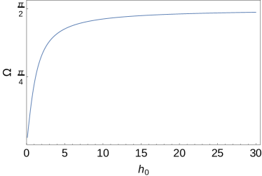
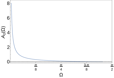
Figure 1: $\Omega$ as a function of $h_{0}$ (left) and $A_{0}$ as a function of $\Omega$ (right). It shows that the function $A_{0}$ diverges at $\Omega=0$ while vanishes at $\Omega=\frac{\pi}{2}$.

One observes that qualitatively $A_{0}$ diverges at $\Omega=0$ while vanishes at $\pi/2$. To make this statement more precise we have numerically studied asymptotic behaviours of the function $A_{0}$ for $\Omega\rightarrow 0$ and $\Omega\rightarrow\frac{\pi}{2}$ limits as shown in Fig 2.

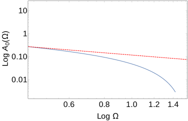
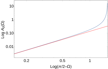
Figure 2: Asymptotic behaviours of $A_{0}$ at $\Omega\rightarrow 0$ (left) and $\Omega\rightarrow\frac{\pi}{2}$(right). In these plots the dashed lines correspond to test functions to probe the limiting value of $A_{0}$. The corresponding functions are given by $y=-x-2.15$ (left) and $y=2x-2.01$ (right), in agreement with equation (3.31).

The results may be summarized as follows

$$C_{\rm singular}^{\rm EE}=\Bigg{\{}\begin{array}[]{rcl}&\frac{3L^{d}}{4G}\frac{0.116}{\Omega},&\Omega\rightarrow 0,\\ &\frac{3L^{d}}{4G}\frac{1.683}{4\pi}\left(\frac{\pi}{2}-\Omega\right)^{2},&\Omega\rightarrow\frac{\pi}{2}.\end{array}$$ (3.31)

3.5 $d_{\theta}=5$

In this case and when $n\neq 3$ we get

$$C_{\rm singular}^{\rm EE}=\frac{3n^{2}L^{d}}{4G}\;\frac{\left(7n^{2}-64\right)\cos(2\Omega)+n(7n-32)+64}{4096(3-n)}\frac{\cos^{2}\!\Omega}{\sin^{4-n}\!\Omega}$$ (3.32)

while for $n=3$

$$C_{\rm singular}^{\rm EE}=\frac{3L^{d}}{4G}\frac{9(31-\cos 2\Omega)}{4096}\frac{\cos^{2}\Omega}{\sin\Omega}.$$ (3.33)

Therefore the corresponding universal term has the following asymptotic behaviours

$$C_{\rm singular}^{\rm EE}=\Bigg{\{}\begin{array}[]{rcl}&\frac{3n^{2}L^{d}}{4G}\;\frac{2n(7n-16)}{4096(3-n)}\frac{1}{\Omega^{4-n}},&\Omega\rightarrow 0,\\ &\frac{3n^{2}L^{d}}{4G}\frac{32(4-n)}{4096(3-n)}\left(\frac{\pi}{2}-\Omega\right)^{2},&\Omega\rightarrow\frac{\pi}{2},\end{array}$$ (3.36)

with an obvious replacement for $n=3$.

It is also straightforward to further consider higher $d_{\theta}$. The lesson we learn from these explicit examples is that for a singular surface of the form $c_{n}\times\mathbb{R}^{d-n-2}$ and for $d_{\theta}\geq 2$ the coefficient of the universal term given in the equation (3.12) has the following generic asymptotic behaviour

$$C_{\rm singular}^{\rm EE}\sim\Bigg{\{}\begin{array}[]{rcl}&\frac{3L^{d}}{4G}\frac{1}{\Omega^{d_{\theta}-n-1}},&\Omega\rightarrow 0,\\ &\frac{3L^{d}}{4G}\left(\frac{\pi}{2}-\Omega\right)^{2},&\Omega\rightarrow\frac{\pi}{2}.\end{array}$$ (3.39)

We see that for a generic opening angle $\Omega$, we can infer the following expression for the coefficient of the universal term

$$C_{\rm singular}^{\rm EE}=f_{d_{\theta},n}(\Omega)\;\frac{3L^{d}}{4G}\;\frac{\cos^{2}\!\Omega}{\sin^{d_{\theta}-n-1}\!\Omega},$$ (3.40)

where $f_{d_{\theta},n}(\Omega)$ is a function of $\Omega$ which is fixed for given $d_{\theta}$ and $n$ by requiring it to be finite at $\Omega=0$ and $\Omega=\frac{\pi}{2}$.

4 New charge

In the previous section we showed that the area of minimal surfaces ending on singular entangling regions may present logarithmic divergences for specific choices of the extension of the singularity, the dimensionality of the space time and the value of $\theta$. The coefficients of these divergent terms depend on the opening angle of the region, and we were able to compute their value in the nearly smooth limit.

Based on these results and using the general expression given in the equation (3.12) for $d_{\theta}\geq 2$ one may define a new charge as follows

$$C_{d}^{n}=\lim_{\Omega\rightarrow\frac{\pi}{2}}\;\frac{C_{\rm singular}^{\rm EE}}{\cos^{2}\Omega}.$$ (4.1)

Note that this is a well defined limit, leading to a finite quantity which is proportional to $\frac{L^{d}}{G}$ up to a numerical factor of order of one. Note also that as soon as we fixed $d_{\theta}$ the resulting charge is independent of $\theta$, and may be defined in any dimension by setting $n=d_{\theta}-2$.

As we have already mentioned there is another central charge which could be defined in any dimension: the coefficient of the $<TT>$ two point function of the stress-energy tensor, which we denote by $C_{T}$. Following the idea of [16, 15], we can compare these two charges. Unlike two dimensional CFT where $C_{T}$ is the same as the one appearing in the central extension of the Virasoro algebra, in higher dimensions it should be read from the explicit expression of the two point function. Indeed, in the present context, the corresponding two point function may be found from the quadratic on-shell action of the perturbation of the metric above a vacuum solution using holographic renormalization techniques[29].

We note, however, that since we do not have a well defined asymptotic behaviour of metric (A.6) in the sense of Fefferman-Graham expansion, in general it is not an easy task to compute the stress-energy tensor’s two point function for spacetimes with generic $\theta$ and $z$. Nevertheless setting $z=1$, where one recovers the Lorentz invariance, we can still use the holographic renormalization procedure to find (see Appendix A)

$$C_{T}=\frac{L^{d}}{8\pi G}\;\;\frac{d+2}{d}\;\frac{\Gamma(d_{\theta}+2)}{\pi^{\frac{d+1}{2}}\Gamma\left(\frac{1+2d_{\theta}-d}{2}\right)}.$$ (4.2)

Note that for $z=1$, from the null energy condition one gets $\theta(d-\theta)\leq 0$ which has only a partial overlap with the parameter space of the model we are considering at $\theta=0$. Therefore using the above expression we really should only compare it with the new central charge of the model for $\theta=0$.
Since however the new charge defined in (4.1) for given $d_{\theta}$ is independent of $\theta$, the comparison still makes sense. In particular for $d_{\theta}=2,3$ and $d_{\theta}=4$, respectively, one finds:

$$\frac{C_{d}^{0}}{C_{T}}=\frac{d\;\pi^{\frac{d+1}{2}}\Gamma\left(\frac{5-d}{2}\right)}{2(d+2)},\;\;\;\;\;\;\;\;\;\;\;\;\;\;\frac{C_{d}^{1}}{C_{T}}=-\frac{d\;\pi^{\frac{d+3}{2}}\Gamma\left(\frac{7-d}{2}\right)}{64(d+2)},\;\;\;\;\;\;\;\;\;\;\frac{C_{d}^{2}}{C_{T}}=1.683\frac{d\;\pi^{\frac{d+1}{2}}\Gamma\left(\frac{9-d}{2}\right)}{80(d+2)}$$ (4.3)

For $z\neq 1$, $C_{T}$ depends explicitly on $z$ and thus the above ratio will be $z$ dependent, even though $C^{n}_{d}$ will not.

Since both central charges considered above are proportional to $\frac{L^{d}}{G}$, it is evident that their ratio is a purely numerical constant. In [16] it was conjectured that for three dimensional CFTs this ratio could be completely universal, regardless of the strength of the coupling so to hold in both known statistical models and in QFTs with gravity duals. It is thus interesting to understand whether this ratio, which could characterize whatsoever CFT of fixed dimensionality, is still universal even in the higher dimensional cases we are considering.
The easiest step we can make in this direction is to look at gravity theories with higher curvature terms in the action, and see whether the corrections alter the ratio (4.3) .

To proceed let us consider an action containing the most general curvature squared corrections as follows

$$I=-\frac{1}{16\pi G}\int d^{d+2}\sqrt{-g}\bigg{(}R+V(\phi)+\lambda_{1}R^{2}+\lambda_{2}R_{\mu\nu}R^{\mu\nu}+\lambda_{3}R_{\mu\nu\rho\sigma}R^{\mu\nu\rho\sigma}\bigg{)}+I_{\rm matter}$$ (4.4)

where $I_{\rm matter}$ is a proper matter action to make sure that the model admits hyperscaling violating geometry. It is then straightforward, although lengthy, to compute holographic entanglement entropy for this model. Indeed following [31], the holographic entanglement entropy may be obtained by minimizing the following entropy functional

$$S_{A}\!\!=\!\!\frac{1}{4G}\!\int\!d^{d}\zeta\;\sqrt{\gamma}\;\bigg{[}1+2\lambda_{1}R+\lambda_{2}\left({R}_{\mu\nu}n^{\mu}_{i}n^{\nu}_{i}-\frac{1}{2}\mathcal{K}^{i}\mathcal{K}_{i}\right)\!+\!2\lambda_{3}\bigg{(}R_{\mu\nu\rho\sigma}n^{\mu}_{i}n^{\nu}_{j}n^{\rho}_{i}n^{\sigma}_{j}-\mathcal{K}^{i}_{\mu\nu}\mathcal{K}_{i}^{\mu\nu}\bigg{)}\!\bigg{]},$$ (4.5)

where with $i=1,2$ we denote the two transverse directions to a co-dimension two hypersurface in the bulk, $n_{i}^{\mu}$ are two mutually orthogonal unit vectors to the hypersurface and ${\cal K}^{(i)}$ are the traces of two extrinsic curvature tensors defined by

$${\cal K}_{\mu\nu}^{(i)}=\pi^{\sigma}_{\ \mu}\pi^{\rho}_{\ \nu}\nabla_{\rho}(n_{i})_{\sigma},\;\;\;\;\;\;\;{\rm with}\;\;\;\;\pi^{\sigma}_{\ \mu}=\delta^{\sigma}_{\ \mu}+\xi\sum_{i=1,2}(n_{i})^{\sigma}(n_{i})_{\mu}\ ,$$ (4.6)

where $\xi=-1$ for space-like and $\xi=1$ for time-like vectors. Moreover $\gamma$ is the induced metric on the hypersurface whose coordinates are denoted by $\zeta$.

Although so far we have been considering a theory with hyperscaling violation, as we have already mentioned the holographic renormalization for generic hyperscaling exponent has not been fully worked out and thus we have restricted ourselves to to consider backgrounds with $z=1$. In this case the most interesting case allowed by the null energy condition is $\theta=0$. Therefore in what follows we just examine the relation between the two charges for $\theta=0$ in an arbitrary dimension.

To compute higher curvature corrections to the entanglement entropy we note that in our case the normal vectors are given by (note that we set $\theta=0$)

$$n_{1}=\frac{L}{r}\bigg{(}1,0,0,0\cdots\bigg{)}\,,\;\;\;\;\;\;\;n_{2}=\frac{L}{r}\frac{1}{\sqrt{1+h(\varphi)^{2}+h^{\prime}(\varphi)^{2}}}\bigg{(}0,1,-h(\varphi),-\rho h^{\prime}(\varphi),0,\cdots\bigg{)}\,.$$ (4.7)

It is then straightforward to extremize the functional (4.5) and evaluate it. In fact one only needs to expand the above entropy functional around $h=0$ to find its divergences and read the universal coefficient of the logarithmic (or log²) term to find the corrections to the central charge $C_{d}^{n}$. Doing so one arrives at

$$\tilde{C}_{d}^{\,n}=\Upsilon\;C_{d}^{\,n}\,,$$ (4.8)

where $\tilde{C}$ is the corrected central charge and

$$\Upsilon=1+\frac{4(d-2)}{L^{2}}\lambda_{3}-\frac{2(d+1)}{L^{2}}(\lambda_{2}+(d+2)\lambda_{1})\,.$$ (4.9)

Now one needs to compute the corresponding corrections to the central charge $C_{T}$. To do so one first needs to linearize the equations of motion deduced from the action (4.4) (see for example [32])

$$R_{\mu\nu}-\frac{1}{2}g_{\mu\nu}(R+V(\phi))+2\lambda_{1}\left(R_{\mu\nu}-\frac{1}{4}g_{\mu\nu}R\right)R+2\lambda_{2}\left(R_{\mu\sigma\nu\rho}-\frac{1}{4}g_{\mu\nu}R_{\sigma\rho}\right)R^{\sigma\rho}$$ (4.10)

$$+(2\lambda_{1}+\lambda_{2}+2\lambda_{3})\bigg{(}g_{\mu\nu}\Box-\nabla_{\mu}\nabla_{\nu}\bigg{)}R+(\lambda_{2}+4\lambda_{3})\;\Box\left(R_{\mu\nu}-\frac{1}{2}g_{\mu\nu}R\right)$$ (4.11)

$$+2\lambda_{3}\left(2R_{\mu\sigma\nu\rho}R^{\sigma\rho}+R_{\mu\sigma\rho\tau}R_{\nu}^{\sigma\rho\tau}-2R_{\mu\sigma}R^{\sigma}_{\nu}+\frac{1}{4}g_{\mu\nu}(R_{\alpha\beta\rho\sigma}^{2}+4R_{\alpha\beta}^{2})\right)=0$$ (4.12)

Using the notation of Appendix A one can linearize the above equations around the vacuum solution given by (A.6) with $\theta=0$. The result is

$$\Upsilon\;{\cal G}_{\mu\nu}^{(1)}+(2\lambda_{1}+\lambda_{2}+2\lambda_{3})\!\left(\!\bar{g}_{\mu\nu}\bar{\Box}-\bar{\nabla}_{\mu}\bar{\nabla}_{\nu}-\frac{d+1}{L^{2}}\bar{g}_{\mu\nu}\!\right)\!R^{(1)}+(\lambda_{2}+4\lambda_{3})\!\left(\!(\bar{\Box}+\frac{2}{L^{2}}){\cal G}_{\mu\nu}^{(1)}+\frac{d}{L^{2}}\bar{g}_{\mu\nu}R^{(1)}\!\right)\!\!=\!0,$$ (4.13)

where $\Upsilon$ is exactly the one given in equation (4.9), and

$${\cal G}_{\mu\nu}^{(1)}=R_{\mu\nu}^{(1)}-\frac{1}{2}\bar{g}_{\mu\nu}R^{(1)}+\frac{d+1}{L^{2}}h_{\mu\nu}.$$ (4.14)

In the transverse-traceless gauge the above equation reads

$$\left[\Upsilon+(\lambda_{2}+4\lambda_{3})\!\left(\bar{\Box}+\frac{2}{L^{2}}\right)\right]\left(\bar{\Box}+\frac{2}{L^{2}}\right)h_{\mu\nu}=0$$ (4.15)

which has to be solved in order to find the linearized solution. Since we are interested in the correlation function of the energy momentum tensor, we should still look for a solution of $(\bar{\Box}+\frac{2}{L^{2}})h_{\mu\nu}=0$. This equation is exactly the same one gets from purely Einstein gravity, and thus the linearized equation of motion reduces essentially to solving standard linearized Einstein equations. On the other hand, to evaluate the two point function one needs to find the quadratic action which has an effective Newton constant $\Upsilon/G$. Indeed going through the computations of the two point function one finally finds that

$$\tilde{C}_{T}=\Upsilon\;C_{T},$$ (4.16)

and thus we may conclude that

$$\frac{\tilde{C}_{d}^{\,n}}{\tilde{C}_{T}}=\frac{{C}_{d}^{\,n}}{{C}_{T}}.$$ (4.17)

for arbitrary dimensions but with $\theta=0$.
Although we have examined the relation between the two central charges $C_{T}$ and $C_{d}^{\,n}$ just for squared curvature modifications of Einstein gravity, based on our observations and the three-dimensional results of [16], it is tempting to conjecture that the the central charge $C_{d}^{\,n}$ is directly related to $C_{T}$ for a generic CFT.

5 Conclusions

In this paper we have studied the holographic entanglement entropy of an entangling region $c_{n}\times\mathbb{R}^{d-n-2}$, i.e. an $n$-dimensional cone extended in $d-n-2$ transverse directions, for a $d+1$ dimensional theory in a hyperscaling violating background. We have observed that due to the presence of a corner in the entangling region the divergence structure of the entropy gets new terms.

In particular for certain values of $\theta,d$ and $n$ the divergent terms include log or log-squared terms whose coefficients are universal, in the sense that they are independent of the UV cut off.

Given that we have been able to extract new regularization independent quantities, it is tempting to conjecture that some information can be obtained about the underlying dual field theory. This might be compared with the case of two dimensional conformal field theories where the central charge appears in the coefficient of the (leading) logarithmic divergence of the entanglement entropy for an interval.

Motivated by this similarity we proceed by analogy and, denoting the coefficient of the logarithmic term appearing in the expression for the entanglement entropy by $C_{\rm singular}^{EE}$ (see equation (3.12)), we find that for $d_{\theta}\geq 2$ we can define a new ”central charge” as follows

$$C_{d}^{\,n}=\lim_{\Omega\rightarrow\frac{\pi}{2}}\;\frac{C_{\rm singular}^{\rm EE}}{\cos^{2}\Omega},$$ (5.1)

which is proportional to $L^{d}/G$. As soon as the effective dimension $d_{\theta}$ is fixed, the proportionality constant only depends on $d$ and $n$, while it is independent of $\theta$. Therefore it remains unchanged even if we set $\theta=0$, reducing the dual theory to a $d+1$ dimensional conformal field theory. It is natural to expect that this central charge may provide a measure for the number of degrees of freedom of the theory. Note that, unlike the one obtained from Weyl anomaly, this central charge can be defined for both even and odd dimensions when $d_{\theta}=n+2$.

Another central charge which could be defined in any dimension is the one entering in the expression for the stress-energy tensor’ two point function. We checked whether the ratio between these charges is a pure number and we also have computed corrections to both $C_{d}^{n}$ and $C_{T}$ for theories with quadratic correction in the curvature. We have shown that the relation between these two charges remains unchanged.

Based on this observation and the results for three dimensional CFTs [15, 16], one may conjecture that the relation between these two central charges ( $C_{T}$ and $C_{d}^{n}$) is a somehow intrinsic property of the field theory. In fact this relation is reminiscent of the relation between Weyl anomaly of a conformal field theory in even dimension and the logarithmic term in the entanglement entropy of the corresponding theory. If there is, indeed, such a relation one would expect to have a general proof for it independently of an explicit example[34].

Appendix

Appendix A Backgrounds with hyperscaling violating factor

In this section we will review certain features of gravitational backgrounds with hyperscaling violating factor[18, 19, 21]. In what follows we will follow the notation of [35] and consider a minimal dilaton-Einstein-Maxwell action, that is

$$S=-\frac{1}{16\pi G}\int d^{d+2}x\sqrt{-g}\left[R-\frac{1}{2}(\partial\phi)^{2}+V(\phi)-\frac{1}{4}e^{\lambda\phi}F_{\mu\nu}F^{\mu\nu}\right],$$ (A.1)

where, motivated by the typical exponential potentials of string theories, we will consider the following potential

$$V=V_{0}e^{\gamma\phi}.$$ (A.2)

The equations of motion of the above action read

$$R_{\mu\nu}+\frac{V(\phi)}{d}g_{\mu\nu}=\frac{1}{2}\partial_{\mu}\phi\partial_{\nu}\phi+\frac{1}{2}e^{\lambda\phi}\left(F_{\mu}^{\rho}F_{\rho\nu}-\frac{g_{\mu\nu}}{2d}F^{2}\right),$$ (A.3)

(A.4)

$$\nabla^{2}\phi=-\frac{dV(\phi)}{d\phi}+\frac{1}{4}\lambda e^{\lambda\phi}F^{2},\;\;\;\;\;\;\partial_{\mu}\left(\sqrt{-g}e^{\lambda\phi}F^{\mu\nu}\right)=0.$$ (A.5)

It is straightforward to find a solution to these equation, namely the black brane

$$ds^{2}=\frac{L^{2}}{r^{2}}\;\left(\frac{r}{r_{F}}\right)^{2\frac{\theta}{d}}\left(-\frac{f(r)dt^{2}}{r^{2(z-1)}}+\frac{dr^{2}}{f(r)}+d\vec{x}_{d}^{2}\right),\;\;\;\;\;\;\;\;f(r)=1-m\;r^{d_{\theta}+z},$$ (A.6)

(A.7)

$$F_{tr}=\sqrt{2(z-1)(d_{\theta}+z)}r^{d_{\theta}+z-1},\;\;\;\;\;\;\;\;\;\;\;\;\;\;\;\;\;\;\;\;\;\;\;\;\phi=\sqrt{2d_{\theta}(z-1-{\theta}/{d})}\log r.$$ (A.8)

which solve (A.3) if we choose the parameters in the action to be

$$V=\frac{(d_{\theta}+z)(d_{\theta}+z-1)}{L^{2}}\left(\frac{r_{F}}{r}\right)^{\frac{2\theta}{d}}\!,\;\;\;\;\;\lambda=-2\frac{\theta+dd_{\theta}}{\sqrt{2dd_{\theta}(dz-d-\theta)}},\;\;\;\;\;\gamma=\frac{2\theta}{d\sqrt{2d_{\theta}(z-1-{\theta}/{d})}}.$$ (A.9)

Here $L$ is the radius of curvature of the spacetime and $r_{F}$ is a scale which can be interpreted as the gravitational dual of the Fermi radius of the theory living on the boundary. A charged black brane solution would need more gauge fields to support its charge, although in what follows we restrict ourselves to the neutral background.

This geometry is a black brane background whose Hawking temperature is

$$T=\frac{d_{\theta}+z}{4\pi\;r_{H}^{z}},$$ (A.10)

where $r_{H}$ is the horizon radius defined by $f(r_{H})=0$. In terms of the Hawking temperature the thermal entropy can be computed to be

$$S_{\rm th}=\left(\frac{4\pi}{d_{\theta}+z}\right)^{\frac{d_{\theta}}{z}}\;\frac{L^{d}V_{d}}{4G\;r_{F}^{d-d_{\theta}}}\;T^{\frac{d_{\theta}}{z}}.$$ (A.11)

It is also interesting to evaluate the quadratic action for a small perturbation above the vacuum solution (A.6). This may be used to compute two point function of the energy momentum tensor. To proceed we will consider a perturbation over the vacuum in which we let vary only the metric

$$g_{\mu\nu}=\bar{g}_{\mu\nu}+h_{\mu\nu},\;\;\;\;\;\;\;\phi=\bar{\phi},\;\;\;\;\;\;\;\;\;A_{\mu}=\bar{A}_{\mu}.$$ (A.12)

where the “bar” quantities represent the vacuum solution (A.6). It is then straightforward to linearize the equations of motion, leading to

$$R_{\mu\nu}^{(1)}+\frac{V(\bar{\phi})}{d}h_{\mu\nu}=0,\;\;\;\;\;\;\;\;\frac{1}{\sqrt{\bar{g}}}\partial_{\mu}\left(\sqrt{\bar{g}}h^{\mu\nu}\partial_{\nu}\bar{\phi}\right)=\frac{1}{2}\bar{g}^{\mu\nu}\partial_{\mu}h\partial_{\nu}\bar{\phi},\;\;\;\;\;\;\;\;\;\bar{F}^{\mu\nu}\partial_{\mu}h=0.$$ (A.13)

Here the linearized Ricci tensor is given by

$$R_{\mu\nu}^{(1)} = \frac{1}{2}\left(-\bar{\nabla}^{2}h_{\mu\nu}-\bar{\nabla}_{\mu}\bar{\nabla}_{\nu}h+\bar{\nabla}_{\sigma}\bar{\nabla}_{\nu}h^{\sigma}_{\mu}+\bar{\nabla}_{\sigma}\bar{\nabla}_{\mu}h^{\sigma}_{\nu}\right)$$

$$= \frac{1}{2}\left(-\bar{\nabla}^{2}h_{\mu\nu}-\bar{\nabla}_{\mu}\bar{\nabla}_{\nu}h+\bar{\nabla}_{\nu}\bar{\nabla}_{\sigma}h^{\sigma}_{\mu}+\bar{\nabla}_{\mu}\bar{\nabla}_{\sigma}h^{\sigma}_{\nu}+\bar{R}_{\sigma\nu}h^{\sigma}_{\mu}+\bar{R}_{\sigma\mu}h^{\sigma}_{\nu}-2\bar{R}_{\lambda\mu\sigma\nu}h^{\lambda\sigma}\right).$$

Moreover for the Ricci scalar one gets

$$R^{(1)}=\bar{g}^{\mu\nu}R^{(1)}_{\mu\nu}-\bar{R}_{\mu\nu}h^{\mu\nu}=-\bar{\nabla}^{2}h+\bar{\nabla}_{\mu}\bar{\nabla}_{\nu}h^{\mu\nu}-\bar{R}_{\mu\nu}h^{\mu\nu}.$$ (A.15)

In order to solve the equations of motion one needs to properly fix the gauge freedom. In our case it turns out to be useful to choose a covariant gauge $\nabla^{\mu}h_{\mu\nu}=\frac{1}{2}\nabla_{\nu}h$, which however still does not fix all redundant degrees of freedom. Indeed, we fix the remaining ones by setting $h_{ri}=h=0$ and thus $\nabla^{\mu}h_{\mu\nu}=0$ so that we reduce to a transverse and traceless gauge. It is easy to see, with this constraint and gauge choice, that the equation of motion of the scalar field at first order will be identically satisfied and one only needs to solve the Einstein equations, which, generally, reduce to further equation of motion for a scalar field. Indeed taking into account that

$$\bar{R}_{\mu\sigma}h^{\sigma}_{\nu}=-\frac{1}{d}\left(V(\bar{\phi})+\frac{1}{4}e^{\lambda\bar{\phi}}\bar{F}^{2}\right)h_{\mu\nu}+\frac{1}{2}h^{\sigma}_{\nu}\left(\partial_{\mu}\bar{\phi}\partial_{\sigma}\bar{\phi}+e^{\lambda\bar{\phi}}\bar{F}^{\rho}_{\mu}\bar{F}_{\rho\sigma}\right)$$ (A.16)

and using the transverse-traceless gauge we arrive at

$$\bar{\nabla}^{2}h_{\mu\nu}+2\bar{R}_{\alpha\mu\beta\nu}h^{\alpha\beta}+\frac{1}{2d}e^{\lambda\bar{\phi}}\bar{F}^{2}h_{\mu\nu}-\frac{1}{2}e^{\lambda\bar{\phi}}\bar{F}_{\rho\sigma}\bar{F}^{\rho}_{(\mu}h_{\nu)}^{\sigma}=0.$$ (A.17)

Using the parameters of the vacuum solution, one could in principle solve the above differential equations with given boundary condition. Then by making use of AdS/CFT correspondence from the quadratic action one can compute the two point function of the energy momentum tensor for a strongly coupled field theory whose gravitational dual is provided by a geometry with hyperscaling violating factor using holographic renormalization.
In general (A.17) cannot be solved analytically, and since for $z\neq 1$ we do not have a good control on the asymptotic behaviour of the metric (in ananlogy with the Fefferman-Graham expansion), it is hard to use holographic renormalization techniques (see however [36] for a related issue).

On the other hand, setting $z=1$, and thus recovering Lorentz symmetry in the bulk metric, we can rely on the holographic renormalization to compute the stress-energy tensor two point’s function, namely because the action reduces to a dilaton-Einstein model with a simpler equation of motion

$$\bar{\nabla}^{2}h_{\mu\nu}+2\bar{R}_{\alpha\mu\beta\nu}h^{\alpha\beta}=0.$$ (A.18)

It is however important to note that the null energy condition for $z=1$ implies that $\theta(d-\theta)\leq 0$, that is either $\theta\leq 0$ or $\theta\geq d$. In all our computations we implicitly assumed $d_{\theta}\geq 1$, playing $d_{\theta}$ the role of the effective dimension, although a solution with $\theta>d$ may not be consistent[21].

Moreover, for $\theta=0$ it is clear that all equations reduce to that of Einstein gravity. In particular one gets [33]

$$h_{k}^{l}(r,x)=\frac{\Gamma\left(d+1\right)}{\pi^{\frac{d+1}{2}}\Gamma\left(\frac{1+d}{2}\right)}\int dy^{d+1}\left(\frac{r}{r^{2}+(x-y)^{2}}\right)^{d+1}J^{i}_{k}(x-y)J^{l}_{j}(x-y)P_{ijab}\;h_{ab}(y),$$ (A.19)

where $h_{ab}$ is the boundary value of metric and (see [33])

$$J_{i}^{j}(x)=\delta_{j}^{i}-2\frac{x_{j}x^{i}}{|x|^{2}},\;\;\;\;\;\;P_{ijab}=\frac{1}{2}(\delta_{ia}\delta_{jb}+\delta_{ib}\delta_{ja})-\frac{1}{d+1}\delta_{ij}\delta_{ab}.$$ (A.20)

Since the quadratic on-shell action is a divergent quantity one needs to consider both boundary and counterterms in order to properly compute the two point function. In the present case for $z=1$ the terms of the renormalized action which could contribute to quadratic order perturbatively in the metric are

$$S_{\rm total}=S-\frac{1}{8\pi G}\int d^{d+1}x\sqrt{\gamma}K-\frac{1}{8\pi G}\int d^{d+1}x\sqrt{\gamma}\;\left(\frac{r_{F}}{r}\right)^{\frac{\theta}{d}}\;\frac{d_{\theta}}{L},$$ (A.21)

where $S$ is the original action (A.1). To evaluate the quadratic action it is also useful to note

$$\int d^{d+1}x\sqrt{\gamma}\;K=\partial_{n}\int d^{d+1}x\sqrt{\gamma}=\frac{r}{L}\left(\frac{r_{F}}{r}\right)^{\frac{\theta}{d}}\partial_{r}\int d^{d+1}x\sqrt{\gamma},$$ (A.22)

with

$$\sqrt{\gamma}=\left(\frac{L}{r}\right)^{d+1}\left(\frac{r}{r_{F}}\right)^{\theta+\frac{\theta}{d}}\left(1+\frac{1}{2}h-\frac{1}{4}h^{i}_{j}h^{j}_{i}+\frac{1}{8}h^{2}+\cdots\right).$$ (A.23)

By plugging the linearized solution back into the action one finds (see [33] for more details)

$$S_{\rm total}=\frac{1}{4}\frac{L^{d}}{16\pi G}\;\frac{d+2}{d}\;\frac{\Gamma(d+2)}{\pi^{\frac{d+1}{2}}\Gamma\left(\frac{1+d}{2}\right)}\int d^{d+1}x\;d^{d+1}y\;\frac{h_{ab}(x)G_{abcd}(x,y)h_{cd}(y)}{(x-y)^{2(d+1)}},$$ (A.24)

where $G_{abcd}(x,y)=J_{a}^{i}(x-y)J^{b}_{j}(x-y)P_{ijcd}$. Having found the quadratic on-shell action the two point function of the energy momentum tensor can be found as follows

$$\langle T_{ab}(x)T_{cd}(y)\rangle=\frac{C_{T}}{(x-y)^{2(d+1)}}G_{abcd}(x,y).$$ (A.25)

where

$$C_{T}=\frac{L^{d}}{8\pi G}\;\;\frac{d+2}{d}\;\frac{\Gamma(d+2)}{\pi^{\frac{d+1}{2}}\Gamma\left(\frac{1+d}{2}\right)},$$ (A.26)

For $z=1$ and $\theta\neq 0$ one can still find a solution for the equation of motion and evaluate the quadratic action. In this case going through the all steps mentioned above, one arrives at

$$C_{T}=\frac{L^{d}}{8\pi Gr_{F}^{d-d_{\theta}}}\;\frac{d+2}{d}\;\frac{\Gamma(d_{\theta}+2)}{\pi^{\frac{d+1}{2}}\Gamma\left(\frac{1+2d_{\theta}-d}{2}\right)}.$$ (A.27)

It is worth noting that the above expression may also be found from the fact that the equations of motion of metric perturbations in traceless-transverse gauge reduce to the equation of motion for a scalar field and therefore the corresponding two point function may be read from the one of a scalar field [21].

For $z\neq 1$, although it is not possible to find holographically the general form of the two point function of $T_{\mu\nu}$, we may still have a chance to compute the equal time correlator. Although we have not gone through the details of this idea, but from the analogous results of the scalar field [21] one might expect to get the following expression

$$C_{T}\propto\frac{L^{d}}{8\pi Gr_{F}^{d-d_{\theta}}}\frac{\Gamma(d_{\theta}+z+1)}{\pi^{\frac{d+1}{2}}\Gamma\left(\frac{2z-1+2d_{\theta}-d}{2}\right)}.$$ (A.28)

We see that here, differently from the holographic entanglement entropy, the coefficient does in fact depend on the Lifshiz exponent $z$.

Appendix B Explicit expressions for $\varphi_{2i}$ and $a_{2i}$ for $i=1,2,3$

In this appendix we will present the explicit form of the coefficients $\varphi_{2i}$ for the first few orders. To proceed let us start with the following series Ansatz for $\varphi$

$$\varphi(h)=\Omega+\varphi_{2}h^{2}+\varphi_{4}h^{4}+\varphi_{6}h^{6}+{\cal O}(h^{8}).$$ (B.1)

Plugging this series in the equation of motion of $\varphi$ one arrives at the equation (2.10) which can be solved order by order. Doing so one finds

$$\varphi_{2}=-\frac{n\cot\Omega}{2(d_{\theta}-1)},\;\;\;\;\varphi_{4}=-\frac{n\cot\Omega[(-2n+(d_{\theta}-1)^{2})n\cot^{2}\Omega+(d_{\theta}-1)^{2}(6-2d_{\theta}+n)]}{8(d_{\theta}-3)(d_{\theta}-1)^{3}},$$ (B.2)

(B.3)

$$\varphi_{6}=-\frac{8(d_{\theta}+2)n^{2}-22(d_{\theta}-1)^{2}n+(3d_{\theta}-7)(d_{\theta}-1)^{3}}{48(d_{\theta}-5)(d_{\theta}-3)(d_{\theta}-1)^{5}}\;n^{3}\cot^{5}\Omega$$ (B.4)

(B.5)

$$\;\;\;\;\;\;\;\;\;-\frac{2(d_{\theta}(d_{\theta}+3)-20)n-(3d_{\theta}-13)(d_{\theta}-1)^{2}-11n^{2}}{24(d_{\theta}-5)(d_{\theta}-3)(d_{\theta}-1)^{3}}\;n^{2}\cot^{3}\Omega$$ (B.6)

(B.7)

$$\;\;\;\;\;\;\;\;\;-\frac{(2d_{\theta}-n-6)(4d_{\theta}-n-20)}{48(d_{\theta}-5)(d_{\theta}-3)(d_{\theta}-1)}\;n\cot\Omega.$$ (B.8)

It is clear from these expressions that the solution breaks down for $d_{\theta}=2k+1$, $k=0,1,\cdots$. In this case one needs to modify the Anstatz by adding a logarithmic term. For example for $d_{\theta}=3$, using the Ansatz

$$\varphi(h)=\Omega+\varphi_{2}h^{2}+\varphi_{4}h^{4}\left(c+\frac{1}{2}\log h^{2}\right)+{\cal O}(h^{6}),$$ (B.9)

one finds

$$\varphi_{2}=-\frac{n}{4}\cot\Omega,\;\;\;\;\;\;\varphi_{4}=-\frac{n^{2}}{64}\left(n-4+n\cos 2\Omega\right)\cot\Omega\csc^{2}\Omega,$$ (B.10)

where $c$ remains unfixed. Similarly for $d_{\theta}=5$ for the Ansatz

$$\varphi(h)=\Omega+\varphi_{2}h^{2}+\varphi_{4}h^{4}+\varphi_{6}h^{6}\left(c+\frac{1}{2}\log h^{2}\right)+{\cal O}(h^{8})$$ (B.11)

one arrives at

$$\varphi_{2}=-\frac{n}{8}\cot\Omega,\;\;\;\;\;\;\varphi_{4}=\frac{n}{512}[(n-8)n\cot^{2}\Omega-8(n-4)]\cot\Omega,$$ (B.12)

(B.13)

$$\varphi_{6}=\frac{(n-4)(7n-16)\;n\cot^{4}\Omega-4(n(11n-40)+32)\cot^{2}\Omega+32(n-4)}{12288}\;n^{2}\cot\Omega,$$ (B.14)

with unspecified $c$.

Having found the coefficients $\varphi_{2i}$ it is straightforward to find the coefficients $a_{2i}$ appearing in the equation (2.17). The results are

$$a_{0}\!\! \!\!=\!\! \!\!\sin^{n}\!\Omega,\;\;\;\;\;\;\;\;\;\;a_{2}=\varphi_{2}(2\varphi_{2}+n\cot\Omega)\sin^{n}\Omega$$ (B.15)

$$a_{4}\!\! \!\!=\!\! \!\!\frac{1}{2}[n\left(2\varphi_{2}^{3}+\varphi_{4}\right)\sin 2\Omega-\varphi_{2}\sin^{2}\Omega\left(\varphi_{2}\left(4\varphi_{2}^{2}+n-4\right)-16\varphi_{4}\right)+\varphi_{2}^{2}(n-1)n\cos^{2}\Omega]\sin^{n-2}\!\Omega.$$

Note that for the particular values of $d_{\theta}=1,3$ one needs to use the proper results of $\varphi_{2i}$ given in this appendix.

References

• [1] P. Calabrese and J. L. Cardy, “Entanglement entropy and quantum field theory,” J. Stat. Mech.  0406, P06002 (2004) [hep-th/0405152].
• [2] J. L. Cardy, “Is There a c Theorem in Four-Dimensions?,” Phys. Lett. B 215, 749 (1988).
• [3] Z. Komargodski and A. Schwimmer, “On Renormalization Group Flows in Four Dimensions,” JHEP 1112, 099 (2011) [arXiv:1107.3987 [hep-th]].
• [4] M. Srednicki, “Entropy and area,” Phys. Rev. Lett.  71, 666 (1993) [hep-th/9303048].
• [5] C. Holzhey, F. Larsen and F. Wilczek, “Geometric and renormalized entropy in conformal field theory,” Nucl. Phys. B 424, 443 (1994) [hep-th/9403108].
• [6] S. Ryu and T. Takayanagi, “Aspects of Holographic Entanglement Entropy,” JHEP 0608, 045 (2006) [hep-th/0605073].
• [7] S. N. Solodukhin, “Entanglement entropy, conformal invariance and extrinsic geometry,” Phys. Lett. B 665, 305 (2008) [arXiv:0802.3117 [hep-th]].
• [8] H. Casini, M. Huerta and R. C. Myers, “Towards a derivation of holographic entanglement entropy,” JHEP 1105, 036 (2011) [arXiv:1102.0440 [hep-th]].
• [9] R. C. Myers and A. Sinha, “Seeing a c-theorem with holography,” Phys. Rev. D 82, 046006 (2010) [arXiv:1006.1263 [hep-th]].
• [10] H. Casini and M. Huerta, “Universal terms for the entanglement entropy in 2+1 dimensions,” Nucl. Phys. B 764, 183 (2007) [hep-th/0606256].
• [11] N. Drukker, D. J. Gross and H. Ooguri, “Wilson loops and minimal surfaces,” Phys. Rev. D 60 (1999) 125006 [hep-th/9904191].
• [12] T. Hirata and T. Takayanagi, “AdS/CFT and strong subadditivity of entanglement entropy,” JHEP 0702, 042 (2007) [hep-th/0608213].
• [13] R. C. Myers and A. Singh, “Entanglement Entropy for Singular Surfaces,” JHEP 1209, 013 (2012) [arXiv:1206.5225 [hep-th]].
• [14] P. Fonda, L. Giomi, A. Salvio and E. Tonni, “On shape dependence of holographic mutual information in AdS4,” JHEP 1502 (2015) 005 [arXiv:1411.3608 [hep-th]].
• [15] P. Bueno, R. C. Myers and W. Witczak-Krempa, “Universality of corner entanglement in conformal field theories,” arXiv:1505.04804 [hep-th].
• [16] P. Bueno and R. C. Myers, “Corner contributions to holographic entanglement entropy,” arXiv:1505.07842 [hep-th].
• [17] D. W. Pang, “Corner contributions to holographic entanglement entropy in non-conformal backgrounds,” arXiv:1506.07979 [hep-th].
• [18] C. Charmousis, B. Gouteraux, B. S. Kim, E. Kiritsis and R. Meyer, “Effective Holographic Theories for low-temperature condensed matter systems,” JHEP 1011, 151 (2010) [arXiv:1005.4690 [hep-th]].
• [19] B. Gouteraux and E. Kiritsis, “Generalized Holographic Quantum Criticality at Finite Density,” JHEP 1112 (2011) 036 [arXiv:1107.2116 [hep-th]].
• [20] L. Huijse, S. Sachdev and B. Swingle, “Hidden Fermi surfaces in compressible states of gauge-gravity duality,” arXiv:1112.0573 [cond-mat.str-el].
• [21] X. Dong, S. Harrison, S. Kachru, G. Torroba and H. Wang, “Aspects of holography for theories with hyperscaling violation,” JHEP 1206, 041 (2012) [arXiv:1201.1905 [hep-th]].
• [22] S. Ryu and T. Takayanagi, “Holographic derivation of entanglement entropy from AdS/CFT,” Phys. Rev. Lett.  96, 181602 (2006) [hep-th/0603001].
• [23] S. Ryu and T. Takayanagi, ”Aspects of Holographic Entanglement Entropy,” JHEP 0608 (2006) 045 [hep-th/0605073].
• [24] N. Ogawa, T. Takayanagi and T. Ugajin, “Holographic Fermi Surfaces and Entanglement Entropy,” JHEP 1201, 125 (2012) [arXiv:1111.1023 [hep-th]].
• [25] M. Alishahiha and H. Yavartanoo, “On Holography with Hyperscaling Violation,” arXiv:1208.6197 [hep-th].
• [26] M. Alishahiha, A. F. Astaneh and M. R. M. Mozaffar, “Thermalization in backgrounds with hyperscaling violating factor,” Phys. Rev. D 90, no. 4, 046004 (2014) [arXiv:1401.2807 [hep-th]].
• [27] P. Fonda, L. Franti, V. Ker nen, E. Keski-Vakkuri, L. Thorlacius and E. Tonni, “Holographic thermalization with Lifshitz scaling and hyperscaling violation,” JHEP 1408, 051 (2014) [arXiv:1401.6088 [hep-th]].
• [28] P. Fonda and E. Tonni, unpublished.
• [29] K. Skenderis, “Lecture notes on holographic renormalization,” Class. Quant. Grav.  19, 5849 (2002) [hep-th/0209067].
• [30] P. Bueno and P. F. Ramirez, “Higher-curvature corrections to holographic entanglement entropy in geometries with hyperscaling violation,” JHEP 1412, 078 (2014) [arXiv:1408.6380 [hep-th]].
• [31] D. V. Fursaev, A. Patrushev and S. N. Solodukhin, “Distributional Geometry of Squashed Cones,” arXiv:1306.4000 [hep-th].
• [32] I. Gullu and B. Tekin, “Massive Higher Derivative Gravity in D-dimensional Anti-de Sitter Spacetimes,” Phys. Rev. D 80, 064033 (2009) [arXiv:0906.0102 [hep-th]].
• [33] H. Liu and A. A. Tseytlin, “D = 4 superYang-Mills, D = 5 gauged supergravity, and D = 4 conformal supergravity,” Nucl. Phys. B 533, 88 (1998) [hep-th/9804083].
• [34] P. Bueno and R. C. Myers, to appear.
• [35] M. Alishahiha, E. O Colgain and H. Yavartanoo, “Charged Black Branes with Hyperscaling Violating Factor,” JHEP 1211, 137 (2012) [arXiv:1209.3946 [hep-th]].
• [36] M. Taylor, “Non-relativistic holography,” arXiv:0812.0530 [hep-th].
• [37] E. Shaghoulian, “A Cardy formula for holographic hyperscaling-violating theories,” arXiv:1504.02094 [hep-th].
• [38] M. H. Dehghani, A. Sheykhi and S. E. Sadati, “Thermodynamics of nonlinear charged Lifshitz black branes with hyperscaling violation,” arXiv:1505.01134 [hep-th].