Edwards thermodynamics for a driven athermal system with dry friction

Abstract

We obtain, using semi-analytical transfer operator techniques, the Edwards thermodynamics of a one-dimensional model of blocks connected by harmonic springs and subjected to dry friction. The theory is able to reproduce the linear divergence of the correlation length as a function of energy density observed in direct numerical simulations of the model under tapping dynamics. We further characterize analytically this divergence using a Gaussian approximation for the distribution of mechanically stable configurations, and show that it is related to the existence of a peculiar infinite temperature critical point.

Although systems governed by dissipative interactions do not obey equilibrium statistical mechanics, there have been several attempts to describe such systems with effective equilibrium-like theories. A paradigmatic example is the problem of amorphous packings of frictional grains, for which an effective thermodynamic was proposed by Edwards and coworkers EO89 ; ME89 ; EM94 ; EG98 ; BHDC15 . This approach relies on the basic assumption that all mechanically stable packings of grains occupying the same volume have the same probability. This is expected if the system is repeatedly perturbed with “extensive operations” EM94 , like a shaking of the grains followed by a fast relaxation to a blocked (mechanically stable) configuration. One can then build an effective thermodynamics by determining all mechanically stable configurations (MSCs) of the grains, and computing the mean values of physical observables from flat averages over accessible blocked configurations. The predicted mean values can then be compared to dynamical averages obtained from a given “tapping” protocol which samples blocked configurations.

For athermal systems in which an energy is defined, Edwards’ prescription can be formulated as follows BKVS00 . One postulates the existence of an effective temperature $T_{\textrm{Ed}}=\beta_{\textrm{Ed}}^{-1}$ such that the probability of a blocked configuration $\mathcal{C}$ of energy $E(\mathcal{C})$ takes the form

$$P(\mathcal{C})=\frac{1}{\mathcal{Z}}\,e^{-\beta_{\textrm{Ed}}E(\mathcal{C})}\,\mathcal{F}(\mathcal{C}),$$ (1)

where $\mathcal{Z}$ is a generalized partition function; $\mathcal{F}(\mathcal{C})=1$ if $\mathcal{C}$ is a MSC and $\mathcal{F}(\mathcal{C})=0$ otherwise (only blocked configurations have a nonzero probability). This constraint is non-Hamiltonian, in the sense that it gives a zero probability to (mechanically unstable) configurations having a finite energy, whereas they would have a finite probability in canonical equilibrium. At first sight, Eq. (1) looks like a harmless generalization of equilibrium statistical mechanics, by simply restricting the set of accessible configurations. For instance, introducing an upper bound $|x_{i}|<X_{\rm max}$ on harmonic oscillators $x_{i}$ does not deeply affect their statistical properties. However, the nontrivial point is that the constraints arising from MSC are often much more complex than simply introducing a bound on individual variables, in particular the constraint of mechanical stability may itself introduce strong correlations in the system. Notice that, beyond volume and energy, one may also take into account other quantities when building an Edwards-type thermodynamics HHC07 ; HC09 ; BE09 ; BJE12 ; BZBC13 (e.g., the stress tensor).

Several attempts have been done to test the Edwards scenario, not only in packings of grains, experimentally NKBJN98 ; SGS05 ; LCDB06 ; NRRCD09 and numerically KM02 ; M04 ; MD05 ; PCN06 ; BK15 , but also, in abstract models like spin and lattice gas BPS00 ; LD01 ; L02 ; BFS02 ; DGL02 ; DGL03 , and in glass and spin-glass models CN00 ; BKVS00 ; BKVS01 ; DL01 ; LD03 . Typically, one uses a specific tapping protocol to sample blocked states, and compares the dynamical average of the observables to the thermodynamic averages obtained from Eq. (1). Although it has been shown explicitly in some cases that Edwards approach is not exact DGL02 ; DGL03 , it is generally believed to be a reasonably good description in many cases BHDC15 . The main difficulty with the Edwards measure Eq. (1) is that the partition function $Z$, from which all thermodynamic quantities can be derived, is very complicated to compute due to the complexity of the function $\mathcal{F}(\mathcal{C})$ characterizing blocked states BE03 ; BE06 ; BSWM08 ; WSJM11 ; APF14 . Standard approaches are then either to consider abstract models BPS00 ; LD01 ; L02 ; BFS02 ; DGL02 ; DGL03 , which are far from any realistic system but simple enough to allow for an explicit solution, or to resort to mean-field SL03 or more involved BE03 approximations, which still capture part of the interesting phenomenology, but (at least partly) miss relevant information about spatial correlations in the system.

In this Letter, we introduce a realistic model in which Edwards thermodynamics can be computed exactly. We investigate a one-dimensional model of frictional blocks connected by harmonic springs, subjected to a tapping dynamics. Due to the one-dimensional geometry, statistical properties can be computed semi-analytically in the thermodynamic limit using a transfer operator method. Our numerical simulation and theoretical results lead both to an infinite temperature critical point, with a correlation length diverging linearly with the stored energy density –a directly measurable quantities in numerical simulations. We analytically confirm these results using a Gaussian approximation for the joint probability distribution of spring elongations, and further characterize this critical point in terms of the divergence of energy and length fluctuations.

Simulations–

Our model is represented by a one-dimensional chain of massive blocks connected by $N$ harmonic springs sliding on a horizontal plane BK67 ; CL89 ; GB10 ; BPG11 ; BGP14 . Each particle is subjected to dry (Coulomb) friction. The position of the $i^{\rm th}$-mass is denoted as $x_{i}$. The effect of dry friction is twofold: when a block is sliding it is subjected to a dissipative force proportional to the dynamic friction coefficient, $f_{i,\textrm{diss}}=-\mu_{\textrm{d}}mg\operatorname{sgn}(\dot{x}_{i})$; when at rest, in order to make it move one has to apply a force larger than the static friction $|f_{i}|>mg\mu_{\textrm{s}}$. We denote $\xi_{i}=x_{i}-x_{i-1}-l_{0}$ the elongation of the spring connecting block $i$ and block $i-1$; $l_{0}$ is the rest length of the spring. Taking into account an external force $f^{\textrm{ext}}_{i}$ the total force exerted on a block is $f_{i}=k(\xi_{i+1}-\xi_{i})+f^{\textrm{ext}}_{i}$, with $k$ the spring stiffness. We write the equation of motion in dimensionless form using the variables $\tilde{t}=t/\tau_{\textrm{0}}$, $\tilde{x}=x/(g\tau_{\textrm{0}}^{2})$, $\tilde{f^{\textrm{ext}}_{i}}=f^{\textrm{ext}}_{i}/(mg)$ and $\tilde{l}_{0}=l_{0}/(g\tau_{\textrm{0}}^{2})$, with $\tau_{\textrm{0}}=\sqrt{k/m}$. We have run simulations of a chain with $N+1=256$ blocks with open boundary conditions – see Supplementary Material (SM). We checked that, over the range of forces explored, no finite size effects appear changing the size from $64$ to $2048$ blocks. Dropping the tildes, the dimensionless equation of motion reads

$$\ddot{x}_{i}=-\mu_{\textrm{d}}\operatorname{sgn}(\dot{x}_{i})+x_{i+1}+x_{i-1}-2x_{i}+f^{\textrm{ext}}_{i},$$ (2)

while the condition to start motion becomes simply $|\xi_{i+1}-\xi_{i}+f^{\textrm{ext}}_{i}|>\mu_{\textrm{s}}$. We identify the “blocked” configurations as those that in absence of external force are mechanically stable: $\forall~{}i$, $\dot{x}_{i}=0$ and $|\xi_{i+1}-\xi_{i}|<\mu_{\textrm{s}}$. We then define the following tapping dynamics: the external forces $f^{\textrm{ext}}_{i}$ are switched on in Eq.(2) and act during a given period of time $\tau$, after which they are switched off and the system relaxes to a MSC. This procedure, that we call driving cycle, is repeated a large number of times to sample MSCs. At each cycle, the forces $f^{\textrm{ext}}_{i}$ are drawn (randomly for each site $i$) from a distribution

$$p(f^{\textrm{ext}}_{i})=(1-\rho)\,\delta(f^{\textrm{ext}}_{i})+\frac{\rho}{\sqrt{2\pi\sigma^{2}}}\,e^{-(f^{\textrm{ext}}_{i}-F)^{2}/2\sigma^{2}}$$ (3)

A driving protocol is determined by fixing the parameters $\rho$ and $\sigma$. For a given protocol, one can then vary the intensity $F$ and duration $\tau$ of the driving. Each MSC is characterized by the typical value of the energy stored by the springs $e=(1/2N)\sum_{i=1}^{N}\xi_{i}^{2}$. For each tapping protocol, the average energy $e(F,\tau)$ of the MCSs is found to depend only on the product $F\tau$ (see SM).

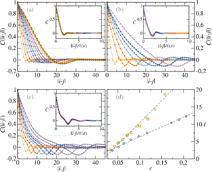
Figure 1: a), b),c): correlation functions $C(|i-j|)$ for different tapping protocols, while in each panel the different curves correspond to different energie values. a) $F\in[20,128]$, $\rho=0.3$, $\sigma=0$; b) $F\in[20,140]$, $\rho=0.8$, $\sigma=0$; c) $F\in[20,128]$, $\rho=1$, $\sigma=F/4$. $\tau=60$ in all simulations. Inset: $C(|i-j|)$ vs. $|i-j|/\ell(e)$, showing a good collapse of the different curves. d): correlation length $\ell(e)$ as a function of the energy density $e$ of the MSC, for the different tapping protocols shown in a) diamonds, b) circles and c) squares, showing a linear increase $\ell(e)\propto e$ with a protocol-dependent slope.

To characterize the MSC we focus on the correlation function $C(|i-j|)=\langle\xi_{i}\xi_{j}\rangle$ between the elongations of the springs at position $i$ and $j$ in the chain. Since this function is trivial ($C(|i-j|=C_{0}\delta_{ij}$) in a thermal harmonic chain at all temperatures, any appearance of correlations is a signature of the unusual statistics associated with the non-Hamiltonian constraints. Correlation functions $C(|i-j|)$ measured for different tapping protocols are shown in Fig. 5. For a given tapping protocol we find that the extent of correlations increases when the average energy of the MSC increases. We extract the correlation length $\ell(e)$ for each case as the distance (i.e., number of springs) $|i-j|$ at which the measured correlation function decays below a conventional threshold $C^{*}=0.2$. The insets of Fig. 5a), 5b) and 5c) show the collapse of the correlation function when the $x$ axis is rescaled with $\ell(e)$. Fig. 5d) shows, for all protocols studied, the correlation length growing linearly with the energy $\ell(e)\sim e$; the higher the energy, the more the system is correlated. This result may look puzzling at first sight, since commonly the larger is the energy the smaller is the extent of correlations. The key point to understand the physics of our system is the non-Hamiltonian nature of the constraints defining the MSC. If for a certain $i$ we have $\xi_{i}\gg 1$ (a situation that is typical of a high energy MCS), then, to fulfill the frictional constraint $|\xi_{i+1}-\xi_{i}|<\mu_{\textrm{s}}$, $\xi_{i+1}$ must be close to $\xi_{i}$. The same argument relates $\xi_{i+2}$ to $\xi_{i+1}$, and so on. Therefore, correlations between spring extensions build up in the MSC. We also compare the correlation functions characterizing the blocked states and those at the end of the driving phase (when the force is switched off) and show that the spring-spring correlations are not due to the external driving, but come entirely from the constraint imposed by static friction (see SM).

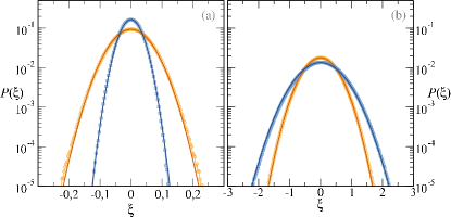
Figure 2: Distributions of springs elongations $P(\xi)$ at different temperatures, on a semi-log scale. Points represent $P(\xi)$ in MSC sampled via tapping, full lines represent $P(\xi)$ obtained from Edwards theory, computed at the temperature $T_{\textrm{Ed}}$ yielding the same energy density $e$ as the tapping. a): uncorrelated regime ($\ell(e)<1$) where $e\sim T_{\textrm{Ed}}$; $T_{\textrm{Ed}}=0.0008$ (blue squares) and $0.0026$ (orange circles). b): correlated regime ($\ell(e)>1$) where $e\sim\sqrt{T_{\textrm{Ed}}}$; $T_{\textrm{Ed}}=1.19$ (orange circles) and $3.84$ (blue squares).

It is interesting to notice that the distribution of spring lengths is Gaussian at all energies. This is shown in Fig. 2, both in the case $\ell(e)<1$, namely when there is no correlation between springs elongations, and in the case $\ell(e)>1$.

Effective theory: transfer operators–

Given that MSC are defined in our model by the constraint $|\xi_{i+1}-\xi_{i}|<\mu_{\textrm{s}}$ $\forall i$, from Eq. (1) the probability of a configuration $\bm{\xi}=(\xi_{1},\ldots,\xi_{N})$ reads

$$P(\bm{\xi})=e^{-\beta_{\textrm{Ed}}\sum_{i=1}^{N}\xi_{i}^{2}/2}\prod_{i=1}^{N}\Theta(\mu_{\textrm{s}}-|\xi_{i+1}-\xi_{i}|).$$ (4)

All the properties of the system can be obtained from the partition sum $\mathcal{Z}=\int_{-\infty}^{\infty}d\xi_{1}\ldots d\xi_{N}~{}P(\bm{\xi})$. Using the change of variables $\xi_{i}=\mu_{\textrm{s}}\xi_{i}^{\prime}$, the partition function depends only (up to an irrelevant prefactor) on the product $\beta_{\textrm{Ed}}\mu_{\textrm{s}}^{2}$; hence, all thermodynamic quantities are functions of $T_{\textrm{Ed}}/\mu_{\textrm{s}}^{2}$. We consider periodic boundary conditions for the chain, without imposing any constraint on its total length. For convenience, we fix the rest length to $l_{0}=\infty$, allowing us to take as domain of integration $\xi_{i}\in(-\infty,\infty)$, while avoiding crossings of masses.

Using Eq. (4), we have $\mathcal{Z}=\textrm{Tr}(\mathcal{T}^{N})$, with $\mathcal{T}$ an operator defined as $\mathcal{T}[f](x)=\int_{-\infty}^{\infty}dy\,T(x,y)f(x)$, being $T(x,y)$ the symmetric function:

$$T(x,y)=e^{-\beta_{\textrm{Ed}}x^{2}/2}\,\Theta(\mu_{\textrm{s}}-|x-y|)\,e^{-\beta_{\textrm{Ed}}y^{2}/2}.$$ (5)

The operator $\mathcal{T}$ has a maximum positive eigenvalue $\lambda_{\textrm{max}}(\beta_{\textrm{Ed}},\mu_{\textrm{s}})$, which can be computed numerically discretizing the domain of $\xi$, and using a complete orthonormal basis in $L^{2}$. All relevant thermodynamic observables are computed in the same way (see SM). The free-energy is obtained as $f=\beta_{\textrm{Ed}}^{-1}\ln(\lambda_{\textrm{max}}(\beta_{\textrm{Ed}},\mu_{\textrm{s}}))$ while the energy reads $e=\partial(\beta_{\textrm{Ed}}f)/\partial\beta_{\textrm{Ed}}=-\langle\lambda_{\textrm{max}}|\partial\mathcal{T}/\partial\beta_{\textrm{Ed}}|\lambda_{\textrm{max}}\rangle/\lambda_{\textrm{max}}$. In the following, we compare results from theory and simulations by tuning the temperature $T_{\textrm{Ed}}$ such that the energy $e$ takes the same value as in the numerics.

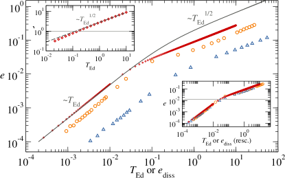
Figure 3: Main : Energy density $e$ of MSC as a function of $T_{\textrm{Ed}}$, from transfer operators (small red diamonds) or Gaussian approximation (full line), and as function of dissipated energy $e_{\textrm{diss}}$ for two tapping protocols: 1) $\rho=0.3$, $\sigma=0$ (orange circles); 2) $\rho=1$, $\sigma>0$ (blue triangles). For $T_{\textrm{Ed}}\ll\mu^{2}$ one finds an “equilibrium-like” regime, $e\sim T_{\textrm{Ed}}$; for $T_{\textrm{Ed}}\gg\mu^{2}$ the behavior is $e\sim\sqrt{T_{\textrm{Ed}}}$. Top inset: Correlation length from exact calculation (transfer operators): the behavior $\ell(T_{\textrm{Ed}})\sim\sqrt{T_{\textrm{Ed}}}\sim e$ is clear when $T_{\textrm{Ed}}\gg\mu^{2}$. Bottom inset: same symbols data sets of main panel are collapsed by just rescaling the $x$-axis: up to a protocol-dependent prefactor we have $e_{\textrm{diss}}\sim T_{\textrm{Ed}}$.

The behavior of energy as a function of $T_{\textrm{Ed}}$ from the transfer operator approach is shown in Fig. 3. We find two regimes separated by a crossover that depends on $\mu_{\textrm{s}}$: for $T_{\textrm{Ed}}\ll\mu_{\textrm{s}}^{2}$ there is an “equilibrium-like” regime where $e\sim T_{\textrm{Ed}}$ while for $T_{\textrm{Ed}}\gg\mu_{\textrm{s}}^{2}$ one finds $e\sim\sqrt{T_{\textrm{Ed}}}$. The transfer operator approach allows us to compute also the probability distribution $p(\xi)$ of the elongation of a single spring (see SM). The theoretical result for $p(\xi)$ is compared in Fig. 2 with the one estimated numerically from the MCSs, showing good agreement. We find that $p(\xi)$ is Gaussian in all regimes, even when correlations are present.

We also compute the correlation $C(|i-j|)=\langle\xi_{i}\xi_{j}\rangle$, which is very close to an exponential form for all values of $T_{\textrm{Ed}}$, $C(|i-j|)\propto e^{-|i-j|/\ell(\beta_{\textrm{Ed}},\mu)}$ (see SM). When $T_{\textrm{Ed}}\gg\mu_{\textrm{s}}^{2}$ both the correlation length $\ell$ and the energy $e$ grow as $\sqrt{T_{\textrm{Ed}}}$ (see inset of Fig. 3), implying $\ell\sim e$. We thus recover from Edwards thermodynamics the scaling behavior of correlation length with energy observed in the simulated tapping dynamics. This is a remarkable success of the Edwards approach for this system. Conversely, there is almost no correlation between neighboring springs ($\ell<1$), in the “equilibrium-like” low energy regime ($e\sim T_{\textrm{Ed}}$).

We further show in the second inset of Fig. 3 that a direct measure of $T_{\textrm{Ed}}$ (within a protocol dependent factor) is obtained from the dissipated energy per tapping cycle and particle, $e_{\mathrm{diss}}=\mu_{d}\langle\int_{0}^{\tau}\mathrm{sgn}(\dot{x}_{i}(t))\dot{x}_{i}(t)dt\rangle$. Indeed, in the simulations $e_{\mathrm{diss}}$ is found to have the same scaling with $e$ as the temperature obtained within the transfer operator approach (i.e., $e\sim e_{\mathrm{diss}}$ if $e\ll\mu_{\textrm{s}}^{2}$, $e\sim\sqrt{e_{\mathrm{diss}}}$ if $e\gg\mu_{\textrm{s}}^{2}$). The dissipated energy can therefore be interpreted as the analog of the thermal energy that allows the system to sample the configuration space Langer .

Effective theory: Gaussian ansatz–

To obtain approximate analytical expressions for the thermodynamic quantities, we replace the Heaviside function in Eq. (4) by a Gaussian function,

$$\Theta(\mu_{\textrm{s}}-|\xi_{i+1}-\xi_{i}|)\;\rightarrow\;\frac{1}{\sqrt{\pi}}\,\exp\left(-\frac{|\xi_{i+1}-\xi_{i}|^{2}}{4\mu_{\textrm{s}}^{2}}\right),$$ (6)

yielding $\mathcal{Z}\propto\int\mathcal{D}{\bm{\xi}}\,e^{-S(\bm{\xi})}$ with an effective Hamiltonian

$$S(\bm{\xi})=\frac{1}{2}\left[\beta_{\textrm{Ed}}\sum_{i=1}^{N}\xi_{i}^{2}+\frac{1}{2\mu_{\textrm{s}}^{2}}\sum_{i=1}^{N}(\xi_{i+1}-\xi_{i})^{2}\right]$$ (7)

This effective Hamiltonian corresponds to a positive definite quadratic form $S(\bm{\xi})=\bm{\xi}^{T}A\bm{\xi}/2$, where $A$ is a symmetric real Toeplitz matrix (see SM). The matrix A can be exactly diagonalized, yielding analytical expressions for energy, entropy, correlation function and correlation length. The mean energy per particle reads

$$e(T_{\textrm{Ed}},\mu_{\textrm{s}})=\frac{1}{2}\frac{\mu_{\textrm{s}}T_{\textrm{Ed}}}{\sqrt{2T_{\textrm{Ed}}+\mu_{\textrm{s}}^{2}}},$$ (8)

from which we recover that the crossover point between the behaviors $e\sim T_{\textrm{Ed}}$ and $e\sim\sqrt{T_{\textrm{Ed}}}$ is $T_{\textrm{Ed}}^{*}\approx\mu_{\textrm{s}}^{2}$. In Fig. 3, Eq. (9) is compared with the result from the transfer operator Eq. (5), showing a semi-quantitative agreement. We also find that the correlation function is $\langle\xi_{i}\xi_{j}\rangle\sim e^{-|i-j|/\ell(T_{\textrm{Ed}},\mu_{\textrm{s}})}$ with $\ell(T_{\textrm{Ed}},\mu_{\textrm{s}})$ such that $\ell\sim\sqrt{T}/\mu_{\textrm{s}}$ in the limit $T_{\textrm{Ed}}\gg\mu_{\textrm{s}}^{2}$. This result can be recovered from a field-theoretic viewpoint, by taking a continuous limit in Eq. (7), yielding

$$S[\xi]\propto\int dx\left[\frac{1}{2}\left(\frac{\partial\xi}{\partial x}\right)^{2}+\frac{1}{2}m^{2}\xi^{2}(x)\right]$$ (9)

with a “mass” term $m^{2}=2\mu_{s}^{2}\beta_{\textrm{Ed}}$. The correlation function of such a Gaussian field theory is known LeBellac to be $\langle\xi(x)\xi(y)\rangle\sim e^{-m|x-y|}$, so that we recover a correlation length $\ell\sim\beta_{\textrm{Ed}}^{-1/2}$. This field-theoretic formulation confirms the presence of an infinite temperature critical point, since the mass term goes to zero at infinite temperature. To inspect the critical exponents associated with this critical point, we study the fluctuations of the total energy of the chain, $\delta E=\frac{1}{2}\sum_{i=1}^{N}(\xi_{i}^{2}-\langle\xi_{i}^{2}\rangle)$ and the fluctuations of its total length $\delta\mathcal{L}=\sum_{i}\xi_{i}$. We find (see SM) that the variance of both energy and length diverge linearly with temperature (or, equivalently, as $\ell^{2}$),

$$\frac{\langle[\delta E]^{2}\rangle}{N}\sim\frac{\langle[\delta\mathcal{L}]^{2}\rangle}{N}\sim T_{\textrm{Ed}}\,.$$ (10)

Finally, we compute the entropy density $s=-\partial f/\partial T_{\textrm{Ed}}$. We find that it saturates at high temperature to a finite value, $\lim_{T_{\textrm{Ed}}\rightarrow\infty}s(T_{\textrm{Ed}},\mu_{\textrm{s}})=\frac{1}{2}\ln 2+\ln\mu_{s}$. This saturation results from the presence of long-range correlation at infinite temperature. This can be confirmed by contrast, computing the “mean-field” entropy density $s_{\rm mf}=-\int d\xi\,p(\xi)\,\ln p(\xi)$, with $p(\xi)$ the distribution of a single spring elongation $\xi$. We find that $s_{\rm mf}$, which discards correlations, diverges like $\ln T_{\textrm{Ed}}$ at infinite temperature (see SM), at odds with the saturation of the entropy $s$.

Conclusions–

The present study provides a clearcut example of how an effective thermodynamic theory can successfully describe an athermal dissipative system. The most remarkable difference between standard equilibrium thermodynamics and the effective theory we have presented is the presence of an infinite temperature critical point, with an associated divergence of the correlation length as $\ell\sim T_{\textrm{Ed}}^{1/2}$ (or $\ell\sim e$). As seen in the field-theoretic formulation Eq. (9), this infinite temperature critical point results from the long-range correlation generated by static friction in the blocked states. The difference with standard equilibrium systems is that the gradient term in the effective Hamiltonian does not come from an energetic interaction, but from a non-Hamiltonian constraint. Its coefficient is strictly temperature independent, while the coefficient of the energetic term scales inversely with temperature. While temperature-independent terms could also be present at equilibrium (e.g., entropic constraints such as excluded volume), they are usually purely local and do not involve gradient terms. Hence, in spite of its simplicity, our model exhibits a phenomenology clearly distinct from that of equilibrium systems, and the field-theoretic formulation suggests that the results should be quite robust to changes in the details of the model. Future work should investigate this issue in more details.

SUPPLEMENTARY MATERIAL:
Edwards thermodynamics for a driven athermal system with dry friction

.1 Numerical simulations

Details on the simulations

The tapping protocol is defined in Eq. (3) in the main text. The motivation for introducing (annealed) disorder in the tapping protocol is that, when taking $\rho=1$ and $\sigma=0$ (i.e., without any disorder in the driving), we found undamped waves which travel across the chain causing an undesired and artificial collapse of the “ensemble” of visited MSC to a very small and specific subset. As mentioned in the main text, for the numerical simulations of the tapping dynamics we consider open boundary conditions. This choice is done in order to avoid constraints on springs which may induce trivial correlations. For instance if one fixes $\sum_{i=1}^{N}\xi_{i}=Nl_{0}$, then also has $N^{2}l_{0}^{2}=\langle L^{2}\rangle=\sum_{ij}\langle\xi_{i}\xi_{j}\rangle$, which is a constraint on the two point correlation function. With open boundary conditions the first and the last blocks are connected to a single spring and their equations of motions are respectively

$$\ddot{x}_{1} = -\mu_{\textrm{d}}\textrm{sgn}{\dot{x}_{1}}+(x_{2}-x_{1}-l_{0})+f^{\textrm{ext}}_{1}$$

$$\ddot{x}_{N+1} = -\mu_{\textrm{d}}\textrm{sgn}{\dot{x}_{N+1}}-(x_{N+1}-x_{N}-l_{0})+f^{\textrm{ext}}_{N+1}$$ (1)

Note that in order to have $N$ springs with open boundary conditions we need $N+1$ blocks.

Dependence of the energy on driving parameters

The average energy of MSC depends in principle on the four parameters which charaterize the driving cycle: the duration $\tau$ of forcing, the intensity of the mean applied force $F$, its standard deviation $\sigma$ as well as the fraction $\rho$ of pulled particles. The parameters $\rho$ and $\sigma$ define the tapping protocol, while $F$ and $\tau$ characterize the intensity of the driving. We have found that for a fixed tapping protocol, the energy $e$ of the dynamically reached MSC does not depends separately on $F$ and $\tau$, but is uniquely determined by the product $F\tau$. This is clearly shown by the set of data reported in Fig. 4.

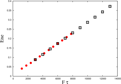
Figure 4: Energy per spring stored in mechanically stable configurations (MSC) as function of $F\tau$ with $F$ the pulling force and $\tau$ the duration of the pulling. Full circles: $F$ is increased at fixed $\tau$; Empty squares: $\tau$ is increased at fixed $F$.

.2 One-cycle experiment: test for the origin of friction induced correlations

In the manuscript we presented data on the “spring-spring” correlation function $\langle\xi_{i}\xi_{j}\rangle$ obtained in the mechanically stable configurations (MSCs). Due to the non-random type of the external force $F$ used to sample different MSCs the reader is allowed to wonder if the correlations we measure in the MSCs are really induced by friction at $100\%$, or a part of them is induced by the same $F$. The numerical evidence that it is not the case comes from the “one-cycle driving experiment” we are going to discuss. The one-cycle driving experiment is analogous to the tapping dynamics discussed in the main text apart from one thing: at the beginning of each driving cycle the positions of blocks are randomized. More precisely all the $x_{i}$ are reset to $x_{i}=i~{}l_{0}+dx$, where $dx$ is normally distributed and $l_{0}$ is the rest length of springs. During the elementary driving cycle of the dynamics a fraction $\rho$ of the particles is pulled for a durantion $\tau$ with a constant force $F$, the force is then switched off and the system relaxes to a MSC. We average over many iterations two correlation functions: a) the forced correlation $\langle\xi_{i}\xi_{j}\rangle_{F}$, which is measured just before switching-off the force at $\tau$; b) The correlation in the mechanically stable configurations reached after the quench, $\langle\xi_{i}\xi_{j}\rangle_{\textrm{MSC}}$. Our aim in studying $\langle\xi_{i}\xi_{j}\rangle_{F}$ is to see how much of the correlation is provided by the external force. On the other hand we must also be sure that when measuring $\langle\xi_{i}\xi_{j}\rangle_{F}$ there is no memory of the correlation in $\langle\xi_{i}\xi_{j}\rangle_{\textrm{MSC}}$ at the previous step. It is for this reason that at the beginning of each driving cycle the positions of block are randomized. In this way we make ourselves sure that if some correlation is measured in $\langle\xi_{i}\xi_{j}\rangle_{F}$, it comes solely from the external force. The result is illustrated in Fig. 5. The continuous line is $\langle\xi_{i}\xi_{j}\rangle_{\textrm{MSC}}$ while the (red) circles represent $\langle\xi_{i}\xi_{j}\rangle_{F}$: being the latter identically zero we can conclude that no correlation is induced by the force and that the correlations we observe in the system come solely from the constraint imposed by static friction on the MSCs.

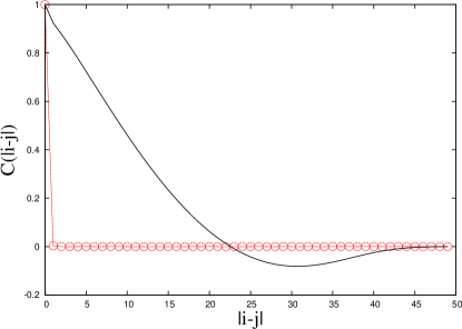
Figure 5: Spring-spring correlation function $\langle\xi_{i}\xi_{j}\rangle_{F}$ (red circles) in presence of the external force and $\langle\xi_{i}\xi_{j}\rangle_{\textrm{MSC}}$ (continuous line) measured in the mechanically stable configurations reached after quench. Data are obtained within a “one-cycle-driving-experiment”: an external constant force $F=100$ is applied for a duration $\tau=100$ pulling a fraction $\rho=0.25$ of the blocks. The number of blocks is $N=256$. At the beginning of each driving cycle the positions of the blocks are randomized.

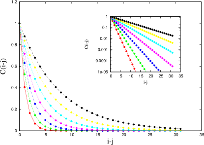
Figure 6: Main: spring-spring correlation function $C(i-j)$, where $i$ and $j$ labels different springs ($i>j$), computed according to Eq. (LABEL:eq:correlation) at different temperatures. From left to right: $T=0.185,0.341,0.631,1.166,2.154,3.981,7.356$. At odds with what usually happens the extent of correlations increases as the temperature is increased. Inset: $C(i-j)$ vs $i-j$ in semi-log scale: all correlations decay exponentially.

.3 Transfer operators

The core of the exact solution of the effective thermodynamics of our model is represented by the spectral properties of the linear operator $\mathcal{T}$, acting in the space of square integrable functions $L^{2}$, $\mathcal{T}:L^{2}\rightarrow L^{2}$. The operator $\mathcal{T}$ is defined as follows:

$$\mathcal{T}[f](x)=\int_{-\infty}^{\infty}dy~{}T(x,y)f(y),$$ (2)

with

$$T(x,y)=e^{-\frac{\beta_{\textrm{Ed}}}{4}y^{2}}\Theta(\mu_{\textrm{s}}-|y-x|)e^{-\frac{\beta_{\textrm{Ed}}}{4}x^{2}}.$$ (3)

As can be easily checked $\int dxdy|T(x,y)|^{2}<\infty$, so that $\mathcal{T}$ is a Hilbert-Schmidt operator, and hence compact and bounded, which guarantees the existence of a maximum positive eigenvalue. The kernel is symmetric and real, $T(x,y)=T^{*}(y,x)$, so that the operator is also self-adjoint, which guarantees the spectral theorem to hold: a complete set of eigenvalues and eigenvectors exist for our operator fonseca .

Correlation function

By means of the transfer operator approach we can compute several quantities of interest: the one that is most relevant for our study is the correlation between the elongation of far apart springs. Let us consider for instance the elongations $\xi_{i}$ and $\xi_{j}$, with $j>i$. In terms of our effective theory the correlation between these two elongations can be written as:

$$\langle\xi_{i}\xi_{j}\rangle = \frac{1}{\mathcal{Z}}\int d\xi_{1}\ldots\xi_{N}T(\xi_{1},\xi_{2})\ldots T(\xi_{i-1},\xi_{i})\xi_{i}T(\xi_{i},\xi_{i+1})$$

$$\dots T(\xi_{j-1},\xi_{j})\xi_{j}T(\xi_{j},\xi_{j+1})\ldots T(\xi_{N},\xi_{1}),$$

which in terms of operators becomes

$$\langle\xi_{i}\xi_{j}\rangle=\frac{1}{\mathrm{Tr}[\mathcal{T}^{N}]}\mathrm{Tr}\left[\mathcal{T}^{i-1}\mathcal{D}\mathcal{T}^{j-i}\mathcal{D}\mathcal{T}^{N-j+1}\right],$$ (5)

where $\mathcal{D}$ is the diagonal operator defined as:

$$\mathcal{D}[f](x)=xf(x).$$ (6)

Exploiting the fact that the operator $\mathcal{T}$ has a complete spectrum of orthonormal eigenvectors we can use the completeness relation $\bm{1}=\sum_{a}|a\rangle\langle a|$, where $|a\rangle$ is the eigenvector of $\mathcal{T}$ relative to the eigenvalue $a$, to simplify Eq. (5). One can write the trace in Eq. (5) as $\mathrm{Tr}(\mathcal{T})=\sum_{a}\langle a|\mathcal{T}|a\rangle$ and then insert between each pair of neighboring operators the completeness $\bm{1}=\sum_{a}|a\rangle\langle a|$. The result is

$$\langle\xi_{i}\xi_{j}\rangle=$$ (7)

$$\frac{1}{\sum_{a}\lambda_{a}^{N}}\sum_{a,b,c,d,e}\langle a|T^{i-1}|b\rangle\langle b|D|c\rangle\langle c|T^{j-i}|d\rangle$$

$$\langle d|D|e\rangle\langle e|T^{N-j+1}|a\rangle$$

$$= \frac{1}{\sum_{a}\lambda_{a}^{N}}\sum_{a,b}\lambda_{a}^{i-1}\langle a|D|b\rangle\lambda_{b}^{j-i}\langle b|D|a\rangle\lambda_{a}^{N-j+1},$$

which in the thermodynamic limit becomes

$$\lim_{N\rightarrow\infty}\langle\xi_{i}\xi_{j}\rangle = \frac{1}{\lambda_{\textrm{max}}^{N}}\sum_{b}\lambda_{\textrm{max}}^{N-j+i}\langle\lambda_{\textrm{max}}|D|b\rangle\lambda_{b}^{j-i}\langle b|D|\lambda_{\textrm{max}}\rangle$$

$$= \sum_{b}\left(\frac{\lambda_{b}}{\lambda_{\textrm{max}}}\right)^{j-i}|\langle b|D|\lambda_{\textrm{max}}\rangle|^{2}$$

$$= \sum_{b}\left(\frac{\lambda_{b}}{\lambda_{\textrm{max}}}\right)^{j-i}\left|\int_{-\infty}^{\infty}dx~{}xf_{{}_{b}}(x)f_{{}_{\lambda_{\textrm{max}}}}(x)\right|^{2},$$

where $f_{{}_{b}}(x)$ is the eigenfunction related to the eigenvalue $b$. The correlation functions obtained at different values of the Edwards temperature $T_{\textrm{Ed}}$ by means of a numerical determination of eigenvalues and eigenvectors of $\mathcal{T}$ can be found in Fig. 6: at all temperatures, we numerically observe an exponential decay, meaning that the second largest eigenvalue dominates the sum in Eq. (LABEL:eq:correlation).

Energy

The average energy of the harmonic chain with $N$ particles is defined as:

$$e_{N}(\beta_{\textrm{Ed}}) = \frac{\partial}{\partial\beta_{\textrm{Ed}}}\left(\beta_{\textrm{Ed}}f\right)=-\frac{1}{N}\frac{\partial}{\partial\beta_{\textrm{Ed}}}\ln(\mathcal{Z})$$ (9)

$$= -\frac{1}{N~{}\textrm{Tr}[\mathcal{T}^{N}(\beta_{\textrm{Ed}})]}~{}\frac{\partial}{\partial\beta_{\textrm{Ed}}}\textrm{Tr}[\mathcal{T}^{N}(\beta_{\textrm{Ed}})]$$

$$= -\frac{1}{\textrm{Tr}[\mathcal{T}^{N}(\beta_{\textrm{Ed}})]}\textrm{Tr}[\mathcal{T}^{N-1}(\beta_{\textrm{Ed}})\frac{\partial\mathcal{T}}{\partial\beta_{\textrm{Ed}}}],$$

where in the last line of Eq. (9) we passed the derivative sign $\partial/\partial\beta_{\textrm{Ed}}$ under the trace sign. The “matrix elements” of the operator $\partial\mathcal{T}/\partial\beta_{\textrm{Ed}}$ are simply defined as the derivative with respect to $\beta_{\textrm{Ed}}$ of the matrix elements of $\mathcal{T}$:

$$\frac{\partial T}{\partial\beta_{\textrm{Ed}}}(x,y)=-\frac{x^{2}+y^{2}}{4}\exp\left(-\frac{\beta_{\textrm{Ed}}}{4}[x^{2}+y^{2}]\right).$$ (10)

Exploiting again the definition of the trace $\mathrm{Tr}[\mathcal{T}^{N}]=\sum_{a}\langle a|\mathcal{T}^{N}|a\rangle$ and by inserting the completeness relation ${\bf 1}=\sum_{a}|a\rangle\langle a|$, we can write

$$e_{N}(\beta_{\textrm{Ed}}) = -\frac{1}{\textrm{Tr}[\mathcal{T}^{N}(\beta_{\textrm{Ed}})]}\textrm{Tr}[\mathcal{T}^{N-1}(\beta_{\textrm{Ed}})\frac{\partial\mathcal{T}}{\partial\beta_{\textrm{Ed}}}]$$

$$= -\frac{1}{\textrm{Tr}[\mathcal{T}^{N}(\beta_{\textrm{Ed}})]}\textrm{Tr}[\mathcal{T}^{N-1}(\beta_{\textrm{Ed}})\cdot{\bf 1}\cdot\frac{\partial\mathcal{T}}{\partial\beta_{\textrm{Ed}}}]$$

$$= -\frac{1}{\sum_{a}\lambda_{a}^{N}}\sum_{ab}\langle a|\mathcal{T}^{N-1}|b\rangle\langle b|\frac{\partial\mathcal{T}}{\partial\beta_{\textrm{Ed}}}|a\rangle$$

$$= -\frac{1}{\sum_{a}\lambda_{a}^{N}}\sum_{a}\lambda_{a}^{N-1}\langle a|\frac{\partial\mathcal{T}}{\partial\beta_{\textrm{Ed}}}|a\rangle$$

which in the thermodynamic limit yields

$$\lim_{N\rightarrow\infty}e_{N}(\beta_{\textrm{Ed}}) = -\frac{1}{\lambda_{\textrm{max}}}\langle\lambda_{\textrm{max}}|\frac{\partial\mathcal{T}}{\partial\beta_{\textrm{Ed}}}|\lambda_{\textrm{max}}\rangle$$

$$= -\frac{1}{\lambda_{\textrm{max}}}\int_{-\infty}^{\infty}dxf_{{}_{\lambda_{\textrm{max}}}}(x)\partial_{\beta_{\textrm{Ed}}}\mathcal{T}(x,y)f_{{}_{\lambda_{\textrm{max}}}}(y),$$

where $f_{\lambda_{\textrm{max}}}(y)$ is the eigenfunction related to the maximum eigenvalue.

Marginal distributions

By means of the transfer matrix technique is easy to obtain marginal distributions. For instance we are interested in the probability distribution of the springs elongation, which reads

$$P_{N}(\xi) = \frac{1}{\mathcal{Z}}\int d\xi_{2}\ldots\xi_{N}~{}T(\xi,\xi_{2})\ldots T(\xi_{N},\xi)$$

$$= \frac{1}{\mathcal{Z}}\langle\xi|\mathcal{T}^{N}|\xi\rangle$$

$$= \frac{1}{\sum_{a}\lambda_{a}}\sum_{ab}\langle\xi|a\rangle\langle a|\mathcal{T}^{N}|b\rangle\langle b|\xi\rangle$$

$$= \frac{1}{\sum_{a}\lambda_{a}^{N}}\sum_{a}\lambda_{a}^{N}|\langle a|\xi\rangle|^{2}$$

$$\lim_{N\rightarrow\infty}P_{N}(\xi) = |f_{{}_{\lambda_{\textrm{max}}}}(\xi)|^{2},$$ (13)

where, again, $f_{{}_{\lambda_{\textrm{max}}}}(x)$ is the eigenfunction related to the maximum eigenvalue. This distribution, which has a Gaussian shape, is plotted for different values of $T_{\textrm{Ed}}$ in Fig.2 in the Letter.

.4 Gaussian approximation

An explicit computation of how the internal energy depends on the temperature is possible if one assumes a Gaussian smoothening of the Heaviside function enforcing the static friction constraint:

$$\Theta(\mu_{\textrm{s}}-|\xi_{i+1}-\xi_{i}|)\Longrightarrow\frac{1}{\sqrt{\pi}}\exp\left(-\frac{|\xi_{i+1}-\xi_{i}|^{2}}{4\mu_{\textrm{s}}^{2}}\right)$$ (14)

With this approximation the whole partition function reads

$$\mathcal{Z} = \pi^{-N/2}\int\mathcal{D}\bm{\xi}e^{-S(\bm{\xi})}$$ (15)

$$= \pi^{-N/2}\int d\xi_{1}\ldots d\xi_{N}~{}~{}\exp\left[-\frac{1}{2}\bm{\xi}\cdot\mathbf{A}\bm{\xi}\right]$$

where $\bm{\xi}$ represents the vector $\bm{\xi}=(\xi_{1},\ldots,\xi_{N})$ and $\mathbf{A}$ is a $X\times N$ symmetric real Toeplitz matrix of the kind

$$\mathbf{A}=\left(\begin{array}[]{cccccc}A_{0}&A_{1}&0&0&0&A_{1}\\ A_{1}&A_{0}&A_{1}&0&0&0\\ 0&A_{1}&A_{0}&A_{1}&0&0\\ 0&0&A_{1}&A_{0}&A_{1}&0\\ 0&0&0&A_{1}&A_{0}&A_{1}\\ A_{1}&0&0&0&A_{1}&A_{0}\\ \end{array}\right)$$

with

$$A_{0} = \beta_{\textrm{Ed}}+\frac{1}{\mu_{\textrm{s}}^{2}}$$

$$A_{1} = -\frac{1}{2\mu_{\textrm{s}}^{2}}$$ (16)

For this kind of matrix the eigenvalues can be explicilty written as

$$\lambda_{k}(\beta_{\textrm{Ed}},\mu_{\textrm{s}}) = A_{0}+2A_{1}\cos\left(\frac{2\pi k}{N}\right)$$ (17)

$$= \beta_{\textrm{Ed}}+\frac{1}{\mu_{\textrm{s}}^{2}}\left[1-\cos\left(\frac{2\pi k}{N}\right)\right].$$

Free energy, energy and entropy

The free-energy reads then as

$$f = -\frac{1}{\beta_{\textrm{Ed}}N}\ln\left(\pi^{-N/2}\int d\xi_{1}\ldots d\xi_{N}~{}~{}\exp\left[-\frac{1}{2}\bm{\xi}\cdot A\bm{\xi}\right]\right)$$ (18)

$$= \frac{\ln 2}{2\beta_{\textrm{Ed}}}+\frac{1}{2\beta_{\textrm{Ed}}N}\ln\det(A)$$

$$= \frac{\ln 2}{2\beta_{\textrm{Ed}}}+\frac{1}{2\beta_{\textrm{Ed}}N}\sum_{k}\ln[\lambda_{k}(\beta_{\textrm{Ed}},\mu_{\textrm{s}})].$$

In the continuous limit

$$\frac{1}{N}\sum_{k=1}^{N}\sim\int_{0}^{1}dk$$ (19)

the free-energy can be exactly computed and reads:

$$f = \frac{\ln 2}{2\beta_{\textrm{Ed}}}+\frac{1}{2\beta_{\textrm{Ed}}}\int_{0}^{1}dk~{}\ln\left(\beta_{\textrm{Ed}}+\frac{1}{\mu_{\textrm{s}}^{2}}\left[1-\cos\left(2\pi k\right)\right]\right)$$

$$= \frac{\ln 2}{2\beta_{\textrm{Ed}}}+\frac{1}{2\beta_{\textrm{Ed}}}\left[\ln\left(\frac{\beta_{\textrm{Ed}}}{4}\right)+2\ln\left(1+\sqrt{1+\frac{1}{\beta_{\textrm{Ed}}\mu_{\textrm{s}}^{2}}}\right)\right]$$

Note that this method to compute the free-energy is different from the transfer operator method. Here we do not write the partition function as the trace of the $N^{\rm th}$ power of a transfer operator, but we diagonalize exactly the quadratic form appearing in Eq. (15). The partition function is then exactly computed for all $N$ using the Gaussian integral formula, and all eigenvalues of $\mathbf{A}$ contribute to the free-energy (while only the largest eigenvalue of the transfer operator contributes to the free energy in the thermodynamic limit).

The energy per degree of freedom can also be computed:

$$e=\frac{\partial(\beta_{\textrm{Ed}}f)}{\partial\beta_{\textrm{Ed}}} = \frac{1}{2N}\sum_{k=1}^{N}\frac{1}{\beta_{\textrm{Ed}}+\frac{1}{\mu_{\textrm{s}}^{2}}\left[1-\cos\left(\frac{2\pi k}{N}\right)\right]}$$

$$\sim \frac{1}{2}\int_{0}^{1}\frac{dk}{\beta_{\textrm{Ed}}+\frac{1}{\mu_{\textrm{s}}^{2}}\left[1-\cos(2\pi x)\right]}$$

$$= \frac{\mu_{\textrm{s}}}{2\sqrt{2\beta_{\textrm{Ed}}+\beta_{\textrm{Ed}}^{2}\mu_{\textrm{s}}^{2}}}=\frac{1}{2}\frac{\mu_{\textrm{s}}T_{\textrm{Ed}}}{\sqrt{2T_{\textrm{Ed}}+\mu_{\textrm{s}}^{2}}}.$$

Combining Eqs. (LABEL:eq:exact-free-enetemp) and (LABEL:eq:exact-enetemp), the entropy per degree of freedom can be simply obtained as $s(\beta_{\textrm{Ed}})=\beta_{\textrm{Ed}}e(\beta_{\textrm{Ed}})-\beta_{\textrm{Ed}}f(\beta_{\textrm{Ed}})$. One can check that $s(\beta_{\textrm{Ed}})\to\frac{1}{2}\ln 2+\ln\mu_{\textrm{s}}$ when $T_{\textrm{Ed}}\to\infty$. Also, energy fluctuations are given by

$$\frac{\langle[\delta E]^{2}\rangle}{N}=-\frac{\partial^{2}}{\partial\beta^{2}}(\beta f)=\frac{\mu_{\textrm{s}}}{2}\,\frac{1+\beta_{\textrm{Ed}}\mu_{\textrm{s}}^{2}}{2\beta_{\textrm{Ed}}+\beta_{\textrm{Ed}}^{2}\mu_{\textrm{s}}^{2}},$$ (22)

and at high temperature they diverge as $\langle[\delta E]^{2}\rangle/N\sim T_{\textrm{Ed}}$, consistently with Eq. (10) in the main text.

Correlation function

When the probability of a configuration of the system is a multivariate gaussian of the kind

$$P(\bm{\xi})\propto\exp\left(-\frac{1}{2}\sum_{ij}A_{ij}\xi_{i}\xi_{j}\right)$$ (23)

we know that the value of the average correlation between $\xi_{i}$ and $\xi_{j}$ is

$$\langle\xi_{i}\xi_{j}\rangle=\left(A^{-1}\right)_{ij}.$$ (24)

For the problem we are studying $A$ is a tridiagonal Toeplitz matrix, for which the explicit formulae for the elements of the inverse is fonseca :

$$\left(A^{-1}\right)_{ij}=(-1)^{i+j}\frac{A_{1}^{j-i}}{|A_{1}|^{j-i+1}}\frac{U_{i-1}(d)U_{n-j}(d)}{U_{n}(d)},$$ (25)

where $d=A_{0}/(2|A_{1}|)$, and $U_{n}(x)$ is a Chebyshev polynomial of the second kind of degree $n$ in the variable $x$. For such polynomials, a useful identity is known:

$$U_{n}(x)=\frac{\sin\theta(n+1)}{\sin\theta},$$ (26)

where $\theta$ is the complex number such that $x=\cos(\theta)$ and $0\leq\Re(\theta)<\pi$. In our case we have

$$d=A_{0}/(2|A_{1}|)=1+\mu_{\textrm{s}}^{2}\beta_{\textrm{Ed}}>1,$$ (27)

where the last inequality on the right is true for every finite value of the temperature and of the friction coefficient. Therefore the number $\theta$ must be a purely imaginary one, i.e., $\theta=i\alpha$, with $\alpha>0$. For our problem we have therefore that the Chebyshev polynomials are defined according to the two following identities:

$$U_{n}(1+\mu_{\textrm{s}}^{2}\beta_{\textrm{Ed}}) = \frac{\sinh\alpha(n+1)}{\sinh\alpha}$$

$$1+\mu_{\textrm{s}}^{2}\beta_{\textrm{Ed}} = \cosh(\alpha)$$ (28)

Because our problem is in the continuum we are interested in the limit $n\rightarrow\infty$ of the expression in Eq. (25). Let us notice the following:

$$\lim_{n\rightarrow\infty}\frac{U_{n-j}(d)}{U_{n}(d)} = \lim_{n\rightarrow\infty}\frac{\sinh[(n-j+1)\alpha]}{\sinh[(n+1)\alpha]}=e^{-\alpha j}$$

$$U_{i-1}(d) = \frac{\sinh(i\alpha)}{\sinh(\alpha)}$$

$$\lim_{\begin{subarray}{c}i\rightarrow\infty\\ i<j\end{subarray}}\frac{U_{i-1}(d)U_{n-j}(d)}{U_{n}(d)} = \lim_{\begin{subarray}{c}i\rightarrow\infty\\ i<j\end{subarray}}\frac{e^{-\alpha(j-i)}-e^{-\alpha(i+j)}}{2\sinh(\alpha)}$$ (29)

$$= \frac{e^{-(j-i)/\ell}}{2\sinh(\ell^{-1})},$$

where the correlation length $\ell$ in the last row is defined as $\alpha=\ell^{-1}$. In the limit where $\mu_{\textrm{s}}^{2}\beta_{\textrm{Ed}}\ll 1$, namely when the temperature is large compared to the friction coefficient, the correlation length $\ell$ must be large and we can estimate its asymptotic scaling:

$$\cosh(\ell^{-1}) = \mu_{\textrm{s}}^{2}\beta_{\textrm{Ed}}+1$$

$$\mu_{\textrm{s}}^{2}\beta_{\textrm{Ed}}\ll 1~{}~{}~{} \Longrightarrow \mu_{\textrm{s}}^{2}\beta_{\textrm{Ed}}+1\sim 1+\frac{\ell^{-2}}{2}$$

$$\mu_{\textrm{s}}^{2}\beta_{\textrm{Ed}}\ll 1~{}~{}~{} \Longrightarrow \ell\sim\frac{\sqrt{T_{\textrm{Ed}}}}{\mu_{\textrm{s}}}$$ (30)

By recalling that $A_{1}=-1/(2\mu_{\textrm{s}}^{2})$, we can finally write the two-point correlation function as:

$$\langle\xi_{i}\xi_{j}\rangle = (A^{-1})_{ij}=\frac{\mu_{\textrm{s}}^{2}}{\sinh(\alpha)}e^{-\alpha(j-i)}$$

$$= \frac{\mu_{\textrm{s}}^{2}T_{\textrm{Ed}}}{\sqrt{\mu_{\textrm{s}}^{4}+2T_{\textrm{Ed}}\mu_{\textrm{s}}^{2}}}e^{-(j-i)/\ell(\mu_{\textrm{s}},T_{\textrm{Ed}})}$$

$$\langle\xi_{i}\xi_{j}\rangle = 2~{}e(\mu_{\textrm{s}},T_{\textrm{Ed}})~{}e^{-(j-i)/\ell(\mu_{\textrm{s}},T_{\textrm{Ed}})},$$ (31)

where the correlation length is

$$\ell(\mu_{\textrm{s}},T_{\textrm{Ed}})=\frac{1}{\mathrm{arcosh}(1+\mu_{\textrm{s}}^{2}/T_{\textrm{Ed}})}.$$ (32)

which scales for $T_{\textrm{Ed}}\to\infty$ as $\ell(\mu_{\textrm{s}},T_{\textrm{Ed}})\sim\sqrt{T_{\textrm{Ed}}}/\mu_{\textrm{s}}$.

The variance of the fluctuations of the total length $\mathcal{L}=\sum_{i=1}^{N}$ read

$$\langle[\delta\mathcal{L}]^{2}\rangle=\sum_{i,j}\langle\xi_{i}\xi_{j}\rangle\sim N\int_{0}^{\infty}dr\,C(r)$$ (33)

with $C(r)$ defined by $C(|i-j|)=\langle\xi_{i}\xi_{j}\rangle$. Using Eq. (31), we get

$$\langle[\delta\mathcal{L}]^{2}\rangle\sim Ne\int_{0}^{\infty}dr\,\exp(-r/\ell)\sim Ne\ell\sim NT_{\textrm{Ed}}$$ (34)

thus recovering the second equality in Eq. (10) of the main text.

Spring length distribution

The probability $P(\bm{\xi})$ is a multivariate Gaussian, so that the marginal distribution $p(\xi)=\int d\xi_{2}\ldots d\xi_{N}P(\bm{\xi})$ is also a Gaussian:

$$p(\xi)=\frac{1}{\sigma(T_{\textrm{Ed}},\mu_{\textrm{s}})\sqrt{2\pi}}e^{-\frac{\xi^{2}}{2\sigma^{2}(T_{\textrm{Ed}},\mu_{\textrm{s}})}},$$ (35)

with

$$\sigma^{2}(T_{\textrm{Ed}},\mu_{\textrm{s}})=(A^{-1})_{ii}=\frac{\mu_{\textrm{s}}T_{\textrm{Ed}}}{\sqrt{2T_{\textrm{Ed}}+\mu_{\textrm{s}}^{2}}}.$$ (36)

The “mean-field” entropy $s_{\rm mf}$ introduced in the text can be computed as

$$s_{\rm mf} = -\int~{}d\xi~{}p(\xi)~{}\ln[p(\xi)]$$ (37)

$$= \frac{1}{2}+\ln[\sigma(T_{\textrm{Ed}},\mu_{\textrm{s}})\sqrt{2\pi}],$$

which yields the asymptotic result

$$s_{\rm mf}(T_{\textrm{Ed}})\sim\ln T_{\textrm{Ed}}\,,\qquad T_{\textrm{Ed}}\rightarrow\infty\,.$$ (38)

The fact that the entropy of Eq. 37 in the infinite temperature limit diverges, and is then wrong compared to Eq.10 in the Letter, is consistent with the fact that formula in Eq. 37 is approximation which does not take into account the correlations.

References

(1) S. F. Edwards and R. B. S. Oakeshott, Physica A 157, 1080 (1989).
(2) A. Mehta and S. F. Edwards, Physica A 157, 1091 (1989).
(3) S. F. Edwards and C. C. Mounfield, Physica A 210, 279 (1994);
Physica A 210, 290 (1994).
(4) S. F. Edwards and D. V. Grinev, Phys. Rev. E 58, 4758 (1998).
(5) D. P. Bi, S. Henkes, K. E. Daniels, and B. Chakraborty, Ann. Rev. Cond. Matt. Phys. 6, 63 (2015).
(6) A. Barrat, J. Kurchan, V. Loreto, and M. Sellitto, Phys. Rev. Lett. 85, 5034 (2000).
(7) S. Henkes, C. S. O’Hern, and B. Chakraborty, Phys. Rev. Lett. 99, 038002 (2007).
(8) S. Henkes and B. Chakraborty, Phys. Rev. E 79, 061301 (2009).
(9) R. Blumenfeld and S. F. Edwards, J. Phys. Chem. B 113, 3981 (2009).
(10) R. Blumenfeld, J. F. Jordan, and S. F. Edwards, Phys. Rev. Lett. 109, 238001 (2012).
(11) D. P. Bi, J. Zhang, R. P. Behringer, and B. Chakraborty, Europhys. Lett. 102, 34002 (2013).
(12) E. R. Nowak, J. B. Knight, E. Ben-Naim, H. M. Jaeger, and S. R. Nagel, Phys. Rev. E 57, 1971 (1998).
(13) M. Schröter, D. I. Goldman, and H. L. Swinney, Phys. Rev. E 71, 030301(R).
(14) F. Lechenault, F. da Cruz, O. Dauchot, and E. Bertin, J. Stat. Mech. P07009 (2006).
(15) S. McNamara, P. Richard, S. de Richter, G. Le Caër, and R. Delannay, Phys. Rev. E 80, 031301 (2009).
(16) J. Kurchan and H. Makse, Nature 415, 614 (2002).
(17) P. T. Metzger, Phys. Rev. E 70, 051303 (2004).
(18) P. T. Metzger and C. M. Donahue, Phys. Rev. Lett. 94, 148001 (2005).
(19) M. Pica Ciamarra, A. Coniglio, and M. Nicodemi, Phys. Rev. Lett. 97, 158001 (2006)
(20) V. Becker and K. Kassner, arXiv:1506.03288.
(21) J. J. Brey, A. Prados, and B. Sanchez-Rey, Physica A 275, 310 (2000).
(22) A Lefèvre and D. S. Dean, J. Phys. A 34, L213 (2001).
(23) A. Lefèvre, J. Phys. A 35, 9037 (2002)
(24) J. Berg, S. Franz, and M. Sellitto, Eur. Phys. J. B 26, 349 (2002).
(25) G. DeSmedt, C. Godrèche, and J. M. Luck, Eur. Phys. J. B 27, 363 (2002).
(26) G. DeSmedt, C. Godrèche, and J. M. Luck, Eur. Phys. J. B 32, 215 (2003).
(27) A. Coniglio and M. Nicodemi, Physica A 296, 451 (2001).
(28) A. Barrat, J. Kurchan, V. Loreto, and M. Sellitto, Phys. Rev. E 63, 051301 (2001).
(29) D. S. Dean and A. Lefèvre, Phys. Rev. E 64, 046110 (2001).
(30) A. Lefèvre and D. S. Dean, Phys. Rev. Lett. 90, 198301 (2003).
(31) R. Blumenfeld and S. F. Edwards, Phys. Rev. Lett. 90, 114303 (2003).
(32) R. Blumenfeld and S. F. Edwards, Eur. Phys. J. E 19, 23 (2005).
(33) C. Briscoe, C. M. Song, P. Wang, and H. A. Makse, Phys. Rev. Lett. 101, 188001 (2008).
(34) P. Wang, C. M. Song, Y. L. Jin, and H. A. Makse, Physica A 390, 427 (2011).
(35) D. Asenjo, F. Paillusson, and D. Frenkel, Phys. Rev. Lett. 112, 098002 (2014).
(36) Y. Srebro and D. Levine, Phys. Rev. E 68, 061301 (2003).
(37)
R. Burridge and L. Knopoff, Bull. Seismol. Soc. Am. 57, 341 (1967).
(38)
J. M. Carlson and J. S. Langer, Phys. Rev. A 40, 6470 (1989).
(39)
J.-C. Géminard and E. Bertin, Phys. Rev. E 82, 056108 (2010).
(40)
B. Blanc, L.-A. Pugnaloni, and J.-C. Géminard, Phys. Rev. E 84, 061303 (2011).
(41)
B. Blanc, J.-C. Géminard, and L.-A. Pugnaloni, Eur. Phys. J. E 37, 112 (2014).
(42)
J. S. Langer, arXiv:1501.07228.
(43)
M. Le Bellac, ”Quantum and Statistical Field Theory”, Oxford Science Publications (Oxford, 1992).

References

(1) C.M. da Fonseca, J. Petronilho, Numer. Math. 100, 2005.