Exploring Dephasing of a Solid-State Quantum Emitter via Time- and
Temperature- Dependent Hong-Ou-Mandel Experiments

Abstract

We probe the indistinguishability of photons emitted by a semiconductor quantum dot (QD) via time- and temperature- dependent two-photon interference (TPI) experiments. An increase in temporal-separation between consecutive photon emission events, reveals a decrease in TPI visibility on a nanosecond timescale, theoretically described by a non-Markovian noise process in agreement with fluctuating charge-traps in the QD’s vicinity. Phonon-induced pure dephasing results in a decrease in TPI visibility from $(96\pm 4)\,$% at 10 K to a vanishing visibility at 40 K. In contrast to Michelson-type measurements, our experiments provide direct access to the time-dependent coherence of a quantum emitter at a nanosecond timescale.

Bright non-classical light sources emitting single indistinguishable photons on demand constitute key building blocks towards the realization of advanced quantum communication networks Knill et al. (2001); Kiraz et al. (2004); Kok et al. (2007); Gisin and Thew (2007); Kimble (2008). In recent years, single self-assembled quantum dots (QDs) integrated into photonic microstructures turned out to be very promising candidates for realizing such quantum-light sources Michler et al. (2000); Santori et al. (2002); Patel et al. (2008); Ates et al. (2009), and enabled, for instance, a record-high photon indistinguishability of 99.5 % using self-organized InAs QDs under strict-resonant excitation Wei et al. (2014). Further advancement of quantum optical experiments and applications of QDs beyond proof-of-principle demonstrations, however, will certainly rely on deterministic device technologies and should be compatible with scalable fabrication platforms. Furthermore, profound knowledge of the two-photon interference (TPI) is crucial for an optimization of novel concepts and devices in the field of advanced quantum information technology. In this respect, previous experiments utilizing QDs showed that dephasing crucially influences the indistinguishability of the photons emitted by the QD states, while a detailed understanding of the involved processes has been elusive Santori et al. (2004); Varoutsis et al. (2005); Gazzano et al. (2013); Gold et al. (2014). In fact, these experiments revealed the difficulty of giving an adequate measure of the coherence time $T_{2}$ of QDs. They even triggered a debate of how to correctly interpret $T_{2}$ obtained via Michelson interferometry, which typically gives a lower bound for the visibilities observed experimentally in Hong-Ou-Mandel (HOM) -type (Hong et al. (1987)) TPI experiments Santori et al. (2004); Gold et al. (2014); Bennett et al. (2005). A commonly accepted - although not proven - explanation for this apparent discrepancy is the presence of spectral diffusion on a timescale which is long compared to the excitation pulse-separation of a few nanoseconds typically used in HOM studies, but much shorter than the integration times of Michelson experiments. In this context, a more direct experimental access to the time dependent dephasing processes and their theoretical description is highly beneficial Wolters et al. (2013); Stanley et al. (2014).

In this work, we map the coherence of a solid-state quantum emitter in the presence of pure dephasing by means of HOM-type TPI experiments. The timescale of the involved decoherence processes is precisely probed using an excitation sequence at which the temporal pulse-separation $\delta t$ is varried. Additionally, temperature-dependent measurements allow us to independently probe the impact of phonon-induced pure dephasing on the indistinguishabilty of photons.

The quantum emitter studied in our experiments is a single InAs QD grown by metal-organic chemical vapor deposition (MOCVD) which is deterministically integrated within a monolithic microlens Gschrey et al. (2013, 2015) (cf. Fig. 1, see also Supplemental Material for details).

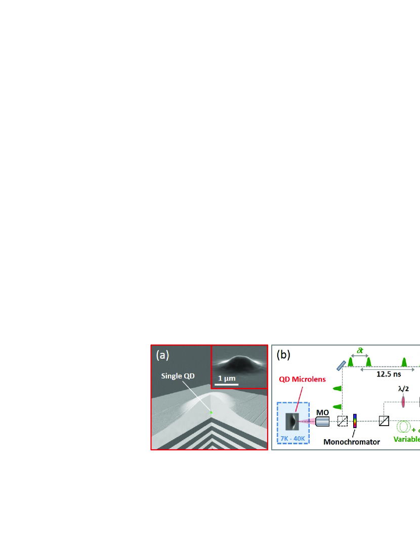
Figure 1: (a) Schematic view of the cross-section of a monolithic microlens with a single deterministically integrated QD. Inset: Scanning electron microscopy image of a fully processed microlens. (b) Experimental setup: Hong-Ou-Mandel-type two-photon interference experiments are utilized to probe the indistinguishability of consecutively emitted photons with variable pulse-separation $\delta t$.

The quantum optical properties of photons emitted by the deterministic QD microlens are studied via low-temperature micro-photoluminescence spectroscopy in combination with HOM-type TPI experiments (cf. Fig. 1 (b), see Supplemental Material for experimental details). A mode-locked Ti:Sapphire laser operating in picosecond mode is used to excite the QD at a repetition rate of 80 MHz. The periodic excitation pulses are converted to a sequence of double-pulses with variable pulse-separation $\delta t$. This excitation scheme in combination with a HOM-type asymmetric Mach-Zehnder interferometer enables us to probe the TPI visibility of two photons emitted by the QD as a function of the time elapsed between consecutive emission events.

A typical micro-photoluminescence ($\mu$PL) spectrum of a deterministic QD microlens chosen for our experiments is depicted in Fig. 2,

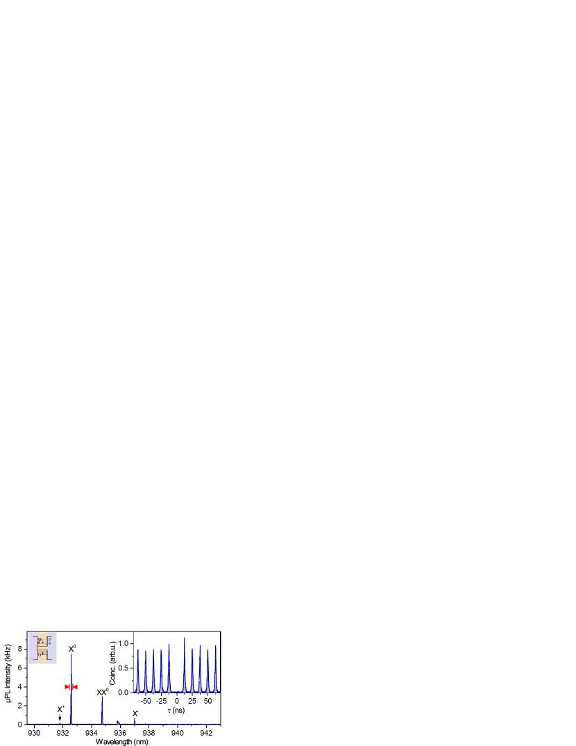
Figure 2: $\mu$PL spectrum of a deterministic QD microlens under p-shell excitation ($T=7\,$K). Inset: Second-order photon-autocorrelation measurement on the X⁰ emission, demonstrating close to ideal single-photon emission.

where the horizontally linearly polarized emission was selected using polarization optics. The QD is excited pulsed ($\delta t=12.5\,$ns) quasi-resonantly in its p-shell at a wavelength of 909 nm. The assignment of the charge neutral exciton (X⁰) and biexciton (XX⁰) states as well as the charged trion states (X⁺, X^-), was carried out via polarization and power dependent measurements as described e.g. in Ref. Schlehahn et al. (2015a). For further investigations we first spectrally selected the emission of the X⁰ state (cf. markers in Fig. 2). The inset of Fig. 2 shows the corresponding raw measurement data of the second-order photon-autocorrelation $g^{(2)}_{\rm{HBT}}(\tau)$.

In contrast to $g^{(2)}_{\rm{HBT}}(0)$, the photon-indistinguishability, being the crucial parameter for advanced quantum communication scenarios, is particular sensitive to dephasing processes. The dephasing rate of a quantum emitter is described by its coherence time $T_{2}$ and the radiative lifetime $T_{1}=\Gamma^{-1}$ via $T_{2}^{-1}=(2T_{1})^{-1}+(T_{2}^{*})^{-1}$ Bylander et al. (2003), where $(T^{*}_{2})^{-1}=\Gamma^{\prime}+\gamma$ describes pure dephasing due to spectral diffusion ($\Gamma^{\prime}$) and phonon interaction ($\gamma$). In the following we gain experimental access to both types of pure dephasing independently by means of time- and temperature dependent TPI experiments.

First, we use a pulse sequence with 12.5 ns pulse-separation. Fig. 3 (a)

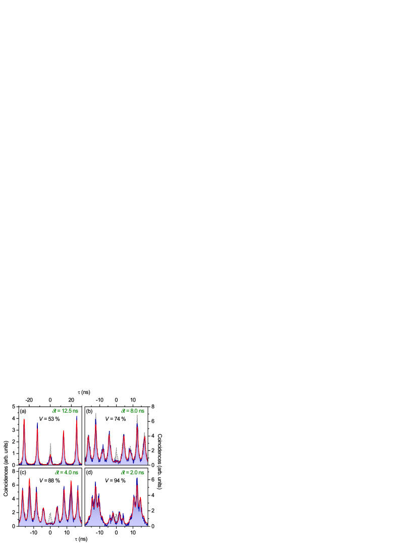
Figure 3: (a) to (d) Two-photon interference histograms measured using a two-pulse excitation sequence with variable pulse-separation $\delta t$ ($T=7\,$K). Data corresponding to co- (cross-) polarized measurement configuration are displayed by solid blue (dashed grey) curve, together with a fit to the data (solid red line) explained in the maintext.

displays the obtained coincidence histogram of the two-photon detection events at the two outputs of the HOM setup. In case of co-polarized photons (solid blue curve), quantum-mechanical TPI manifests in a strongly reduced number of coincidences at $\tau=0$, if compared to the measurement in cross-polarized configuration (dashed grey curve). To quantitatively extract the visibility of TPI, we fitted Lorentzian profiles to the experimental data in co-polarized configuration and evaluated the relative peak areas according to Ref. Santori et al. (2002) (cf. Supplemental Material). Under these excitation conditions, we extract a moderate visibility of $V_{\textup{12.5\,ns}}=(53\pm 8)\,\%$. A possible explanation for the finite wave packet overlap is an inhomogeneous spectral broadening of the QD transition due to spectral diffusion, leading to a pure dephasing rate $\Gamma^{\prime}$ as mentioned above. Such processes are typically characterized by a certain timescale depending on specific material properties and growth conditions Empedocles and Bawendi (1997); Robinson and Goldberg (2000); Türck et al. (2000); Santori et al. (2002); Bennett et al. (2005); Sallen et al. (2010); Houel et al. (2012).

To perform a time-dependent analysis of $\Gamma^{\prime}$ and the underlying dephasing mechanism, we gradually reduce the pulse-separation $\delta t$ (vcf. Fig. 1 (b)), while the respective delay inside the HOM-interferometer is precisely matched to assure proper interference of consecutively emitted single photons. The resulting coincidence histograms for pulse-separations $\delta t$ of 8.0, 4.0 and 2.0 ns are presented in Fig. 3 (b) to (d). The complex coincidence-pulse-pattern specific to each $\delta t$ results from overlapping five-peak structures repeating every 12.5 ns Müller et al. (2014) (see Supplemental Material for details). Fig. 4 (a)

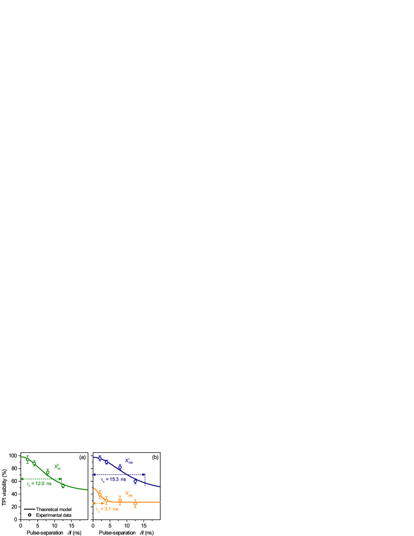
Figure 4: Two-photon interference visibilities of consecutively emitted single photons versus the time $\delta t$ elapsed between the emission processes. Experimental data for (a) the X⁰- and (b) the X⁺-state are quantitatively described by a theoretical model assuming a non-Markovian noise correlation leading to spectral diffusion at a ns-timescale (see Eq. 3). A characteristic temperature-dependent correlation-time $\tau_{c}$ is observed.

summarizes the obtained raw TPI visibilities as a function of the pulse-separation $\delta t$ for the neutral exciton X⁰. At low $\delta t$ a plateau-like behavior is observed, at which the visibility remains almost constant with values of $V_{\textup{2.0ns}}=(94\pm 6)\,\%$ and $V_{\textup{4.0ns}}=(88\pm 4)\,\%$. For pulse-separations larger than 4 ns, a distinct decrease in visibility is observed from $V_{\textup{8.0ns}}=(74\pm 5)\,\%$ to $V_{\textup{12.5ns}}=(53\pm 3)\,\%$. The significant decrease in TPI visibility at pulse-separations larger than 8.0 ns indicates the timescale of spectral diffusion. The time-dependent analysis of $\Gamma^{\prime}$ has additionally been carried out for the charged exciton state X⁺ of the same QD at 10 K and 30 K (cf. Fig. 4 (b)). We observe again a characteristic correlation time, which decreases at higher temperature.

In order to gain deeper insight in the underlying dephasing mechanisms, we model the system with a Hamiltonian (see Supplemental Material), where we approximated the QD as a two-level system with transition energy $\omega_{e}$. To include dephasing, we employ the working horse of the phenomenological dephasing description by including a general stochastic force $F(t)=P(t)+D(t)$ with a phonon-induced dephasing ($\delta$-correlated white noise) $P(t)$ and a spectral diffusion $D(t)$ component (colored noise), both shifting the transition energy of the QD. The specific noise correlations depend on the coupling mechanism between the QD and its environment. For example, in case of spectral diffusion random electric fields due to charge fluctuations induce dephasing Türck et al. (2000); Galperin et al. (2006), as discussed later on. Given that the classical (pump) field excites the QD fast enough to prevent multiple photon emission processes, we calculate via the Wigner-Weisskopf method the wave function after the two pulse sequence:

$$\left|\Psi(t)\right\rangle=\int_{0}^{t}dt_{1}\int_{\delta t}^{t}dt_{2} e^{i(\omega_{e}+i\Gamma)(t_{1}+t_{2})-i\phi_{\delta t}(t_{2})-i\phi_{0}(t_{1})}$$

$$\times E_{2}(t_{2})E_{1}(t_{1})\left|\text{vac}\right\rangle\ .$$ (1)

This wave function includes the two-photon wave packages $E_{n}(t_{n})$ and the time-integrated stochastic forces defined as $\phi^{X}_{i}(t):=\int_{i}^{t}\text{d}t^{\prime}X_{i}(t^{\prime})$, where $i=0$ in case the photon was emitted during the first sequence or $i=\delta t$ for photon emission processes due to the second pulse and $X(t)$ denoting the noise. Considering the interference at the beamsplitter by unitary transformations on the incident electric fields allows us to calculate the two-photon correlation $\left\langle E^{(-)}_{A}(t)E^{(-)}_{B}(t+\tau)E^{(+)}_{B}(t+\tau)E^{(+)}_{A}(t)\right\rangle$ measured in the experiment at detector A and B. To evaluate the stochastic forces, we need to average via a Gaussian random number distribution $\left\langle\left\langle\cdot\right\rangle\right\rangle$. The $\left\langle\left\langle\cdot\right\rangle\right\rangle$ denotes statistical averaging in terms of a Gaussian random variable, where all higher moments can be expressed by the second-order correlation Gardiner and Zoller (2004). Here, we employ the simplest possible model described as a Markovian process $\delta-$correlated in time, i.e. as white noise. It is highly temperature dependent and limits the absolute value of the indistinguishability, independent from the temporal distance of the excitation pulses $\delta t$. In contrast to the phonon-induced dephasing, the spectral diffusion reveals a strong dependence on the pulse distance, as seen Fig. 4. We include this dependence as a finite memory-effect with specific correlation time $\tau_{c}$:

$$\left\langle\left\langle\phi^{D}_{t_{1}}(t_{2})\phi^{D}_{t_{3}}(t_{4})\right\rangle\right\rangle=\int_{t_{1}}^{t_{2}}dt\int_{t_{3}}^{t_{4}}dt^{\prime}\left\langle D(t)D(t^{\prime})\right\rangle$$

$$=\Gamma^{\prime}_{0}\ e^{-\frac{(t_{1}-t_{3})^{2}}{\tau_{c}^{2}}}\left(\text{min}[t_{2},t_{4}]-\text{max}[t_{1},t_{3}]\right)\ ,$$ (2)

where $\Gamma^{\prime}_{0}$ describes the maximal amount of pure dephasing induced by spectral diffusion. These kinds of noise correlations stem from a non-Markovian low-frequency noise Galperin et al. (2006); Laikhtman (1985); Eberly et al. (1984) and show plateau-like behavior for temporal pulse distances sufficiently short in comparison to the memory depth. Thus, if $\delta t\ll\tau_{c}$, the effect of spectral diffusion becomes negligible and phonon-induced dephasing limits the absolute value of the visibility. Using these correlations, assuming a balanced beamsplitter ($R=T=1/2$) and normalizing the two-photon correlation we derive the following formula, which explicitly depends on the pulse-separation $\delta t$:

$$V(\delta t,\tau_{c},T)=\frac{\Gamma}{\Gamma^{\prime}_{0}(1-e^{-(\delta t/\tau_{c})^{2}})+\gamma(T)+\Gamma}\ .$$ (3)

Here, $\Gamma^{\prime}:=\Gamma_{0}^{\prime}(1-e^{-(\delta t/\tau_{c})^{2}})$ corresponds to the $\delta t$-dependent pure dephasing due to spectral diffusion. In case of vanishing phonon-induced dephasing and spectral diffusion, the TPI visibility is $1$, i.e. the photons are Fourier-transform-limited and coalesce at the beamsplitter into a perfect coherent two-photon state. For low temperatures, the phonon-induced dephasing is small and the spectral diffusion with a finite memory depth dictates the functional form of the visibility for different pulse distances.

Applying the model derived in Eq. 3 to the experimental data of Fig. 4, by fixing $\Gamma$ (measured independently via time-resolved measurements) and assuming $\gamma_{\textup{7K,10K}}=0$ (cf. next paragraph), we deduce correlation times $\tau_{c}$ listed in Tab. 1. The timescale at which the noise is correlated appears to be close to the fundamental period of the Ti:Sapphire laser for X${}^{0}_{\textup{7K}}$ and X${}^{+}_{\textup{10K}}$, whereas an increase in temperature to 30 K shortens the correlation time of X⁺ drastically (cf. Tab. 1). Interestingly, the coherence times $T_{2}^{\infty}$ inferred from our model in the limit $\delta t\rightarrow\infty$ (see Tab. 1), significantly exceed the values of $T_{2}=(291\pm 6)\,$ps for X${}^{0}_{7K}$ and $T_{2}=(167\pm 3)\,$ps for X${}^{+}_{30K}$ obtained via measurements using a Michelson-interferometer (see Supplemental Material).

Table 1: Correlation times $\tau_{c}\,$ obtained by fitting Eq. 3 to the experimental data of Fig. 4, fixing $\gamma_{\textup{7K,10K}}=0$ and $\Gamma$. $T_{2}^{\infty}$ values have been calculated from the parameters $\Gamma$, $\Gamma^{\prime}_{0}$ and $\gamma$.

	$\Gamma\,$(GHz)	$\Gamma^{\prime}_{0}\,$(GHz)	$\gamma\,$(GHz)	$\tau_{c}\,$(ns)	$T_{2}^{\infty}\,$(ps)
X${}^{0}_{\textup{7K}}$	0.85	$1.02\pm 0.06$	0	$12.0\pm 1.9$	692
X${}^{+}_{\textup{10K}}$	0.91	$1.03\pm 0.04$	0	$15.3\pm 2.5$	673
X${}^{+}_{\textup{30K}}$	0.96	$1.55\pm 0.78$	$0.29\pm_{0.29}^{1.1}$	$3.1\pm 1.9$	431

A physical origin of the plateau-like behavior of $V(\delta t)$ and the associated non-Markovian decoherence processes are random flips of bistable fluctuators in the vicinity of the QD Laikhtman (1985). Possible candidates for such fluctuators in solid state devices are charge traps or structural dynamic defects Galperin et al. (2006). Further evidence for the presence of charge fluctuations is given by the observation of trion states X⁺ and X^- under quasi resonant excitation of the QD (cf. Fig. 2). To reduce the associated electric field noise, weak optical excitation above-bandgap Gazzano et al. (2013) or a static electric field via gates Stanley et al. (2014) can be applied.

To justify the assumption $\gamma_{\textup{7K,10K}}=0$ and to investigate the influence of phonons on the photon-indistinguishability in more detail, we performed complementary temperature dependent TPI experiments. For this purpose, the emission of the trion state X⁺ was selected under quasi-resonant excitation and coupled to the HOM-interferometer. The pulse-separation was fixed to $\delta t=2.0\,$ns, while the temperature $T$ was varied. Fig. 5 (a) to (c)

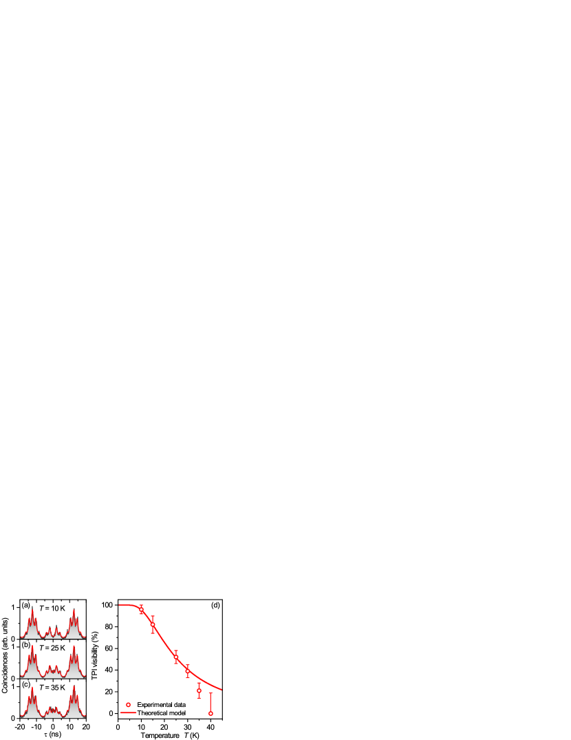
Figure 5: Impact of the temperature on the two-photon interference (TPI) visibiliy ($\delta t=2\,$ns). (a)-(c) TPI histograms for co-polarized configuration at 10, 25 and 35 K and corresponding fits (red solid curves). (d) Experimentally obtained TPI visibilities for various temperatures. We achieve qualitative agreement with a theoretical model assuming dephasing proportional to the phonon number (see Supplemental Material).

exemplarily display TPI coincidence histograms for temperatures $T$ of 10, 25 and 35 K in co-polarized measurement configuration. A gradual increase in coincidences at $\tau=0$ is observed, indicating a reduced photon-indistinguishability. The obtained TPI visibilities extracted from the experimental data for temperatures ranging from 10 to 40 K are depicted in Fig. 5 (d). At low temperature, we observe close to ideal photon-indistinguishability with $V_{\textup{10K}}=(96\pm 4)\,$%. Increasing $T$ results in a distinct decrease of the TPI visibility. Finally, at a temperature of $40\,$K, $V$ approaches zero within the standard error of our measurement. The observed temperature dependence is further modeled theoretically (red solid line). For this purpose we employed a Markovian approximation for the phonon-induced pure dephasing processes, where the dephasing is proportional to the square of the phonon number Carmichael (1999) (see Supplemental Material for details). The model qualitatively describes our experimental observation. Hence, we conclude that the impact of $\gamma$ in Eq. 3 is indeed almost negligible at low temperatures ($T\leq 10\,$K), but has severe impact at elevated temperatures. For temperatures above $30$ K, also in- and outscattering with wetting layer carriers needs to be included, which explains the slight deviation between experiment and theory in this temperature range.

In summary, we presented a method to directly access the time-dependent coherence of a single quantum emitter via HOM-type TPI experiments. We explored the photon-indistinguishability as a function of the time $\delta t$ elapsed between consecutive photon emission events and for different temperatures. We observe TPI visibilities close to unity ($V_{\textup{10K}}=(96\pm 4)\,$%) for MOCVD-grown QDs under p-shell excitation at $\delta t=2.0\,$ns. Increasing $\delta t$ results in a decrease in visibility on a nanosecond timescale. Our theoretical analysis shows that such behavior can be explained by a non-Markovian dephasing process, which is attributed to spectral diffusion caused by fluctuating charge traps. We independently study the impact of phonon-induced pure dephasing on the photon-indistinguishability. Our findings have important implications with respect to the quantum interference of photons emitted by remote emitters Patel et al. (2010); Flagg et al. (2010); Bernien et al. (2012); Gold et al. (2014) and single-photon multiplexing schemes Ma et al. (2011).

Appendix A Supplemental Material

Sample growth and processing: The QD sample utilized for our experiments was grown by metal-organic chemical vapor deposition (MOCVD) on GaAs (001) substrate. A low-density layer of self-organized InGaAs QDs is deposited above a lower distributed Bragg reflector (DBR) constituted of 23 alternating $\lambda/4$-thick bi-layers of AlGaAs/GaAs. On top of the QDs, a 400 nm thick GaAs capping layer provides the material for the subsequent microlens fabrication. To process monolithic single-QD microlenses we used a recently developed deterministic technique exploiting cathodoluminescence (CL) spectroscopy and 3D in-situ electron-beam lithography Gschrey et al. (2013, 2015). Here, the sample is first spin-coated with a 190 nm thick layer of polymethyl methacrylate (PMMA) acting as electron-beam resist. Afterwards, CL intensity maps are recorded in a custom-build CL-system at cryogenic temperature (5 K) and low electron dose. Specific target QDs are then selected for the integration into microlenses. For this purpose, lens-patterns are embossed into the resist by writing concentric circles centered at the target QD’s position, where the applied electron dose is varied from highest values at the center to lowest values at the edge of the microlens. Afterwards, the sample is transfered out of the CL-system, to develop the resist at room temperature. At this point the inverted (unsoluble) PMMA remains above target QDs and acts as a lens-shaped etch-mask, while the resist is completely removed in the remaining CL mapping region. Finally, the microlens profile is transfered into the semiconductor material via dry etching using inductively-coupled-plasma reactive-ion etching (ICP-RIE). An SEM image of a readilly processed microlens is shown in Fig. 1 (a) in the maintext. We have chosen shallow hemispheric microlens sections with heights of 400 nm and base widths of 2.4 $\mu$m, allowing for a photon extraction efficiency of 29 % Schlehahn et al. (2015b).

Experimental setup: The experimental setup is based on $\mu$PL spectroscopy in combination with HOM-type TPI experiments (cf. Fig. 1 (b) in main text). The QD-microlens chip is mounted onto the coldfinger of a liquid-Helium-flow cryostat at cryogenic temperatures $T$ from 7 to 40 K. A mode-locked Ti:Sapphire laser operating in picosecond mode with a repetition rate of 80 MHz is used to quasi-resonantly excite a single QD state in its p-shell. The periodic optical pulses delivered by this laser system are converted to a sequence of double-pulses with pulse-separation of $\delta t$ by utilizing an asymmetric Mach-Zehnder interferometer based on polarization maintaining (PM) single-mode fibers (not shown). By choosing different fiber-delays within one arm of the interferometer, $\delta t$ can be varied from 2.0 ns up to 12.5 ns. This two-pulse sequence is then launched onto a single-QD microlens via a microscope objective (MO) with a numerical aperture of 0.4. The same MO is used to collect and collimate the QD’s emission, which is subsequently focused onto the entrance slit of an optical-grating monochromator with attached charge-coupled device camera (spectral resolution: 0.017 nm (25 $\mu$eV)). Polarization optics (linear polarizer and $\lambda/2$-waveplate) in front of the spectrometer allow for polarization selection of particular QD states. To perform HOM-type TPI experiments, a second PM-fiber-based asymmetric Mach-Zehnder interferometer is attached to the output port of the spectrometer. Using a $\lambda/2$-waveplate, the polarization of the photons in one interferometer arm can be switched either being co- or cross-polarized with respect to the other arm. To interfere consecutively emitted single photons at the second beam-splitter, a variable fiber delay matched to the respective pulse-separation $\delta t$ is implemented in one interferometer arm. The photon arrival time at the second beamsplitter can be fine-tuned with a precision of 3 ps. Finally, photons are detected at the two interferometer outputs using Silicon-based avalanche photodiodes (APDs) and photon coincidences are recorded via time-correlated single-photon counting (TCSPC) electronics enabling coincidence measurements with an overall timing resolution of 350 ps.

Evaluation of Visibility: To extract the TPI visibilities from the coincidence histograms obtained for co-polarized measurement configuration (cf. Fig. 3 in maintext), the peak area ratios can be considered Müller et al. (2014). Fig. 6 schematically illustrates the coincidence pulse patterns resulting from the applied two-pulse sequences with pulse-separations $\delta t$.

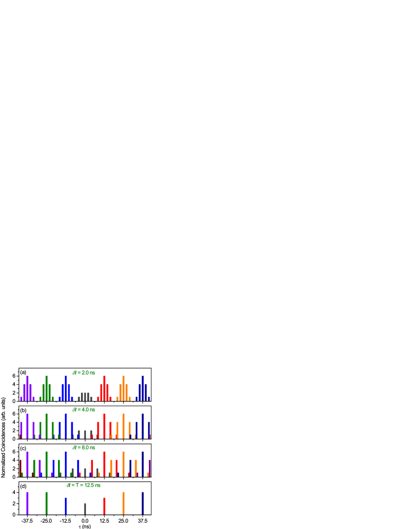
Figure 6: Schematic coincidence pulse patterns resulting from a two-pulse sequence with a pulse-separation $\delta t$ repeating every $T=12.5\,$ns. The expected peak area ratios in case of distinguishable photons are encoded in the the height of each bar.

The peak area ratios deduced from the probability distribution of all possible pathway combinations are represented by the respective bar height. Each pattern is composed of five-peak clusters with temporal delays of $T=12.5\,$ns according to the laser’s fundamental repetition rate. The five-peak cluster in turn arises from the possible pathway-combinations taken by two photons separated by $\delta t$. Thus, the peak area ratios can easily be deduced considering combinatorics, which enables us to extract the TPI visibility quantitatively. The expected peak area ratio of each cluster is 1:4:6:4:1, except for the cluster centered at zero-delay ($\tau=0$). Here, the peak area ratio depends on the photon-indistinguishability. In case of perfect indistinguishability, the coincidences at $\tau=0$ vanish and the peak area ratios of the cluster becomes 1:2:0:2:1. Photons which are distinguishable, e.g. due to their polarization lead to an area ratio of 1:2:2:2:1. In the following, the peak areas of the central cluster are labeled A${}_{2}^{\prime}$:A${}_{1}^{\prime}$:A₀:A₁:A₂ and $\bar{A}=(A_{1}^{\prime}+A_{1})/2$. The corresponding peak areas are extracted from the measurement data by fitting Lorentzian peaks with the expected area ratios to the coincidence histograms. In all fits, we fixed the width of the Lorentzian peaks to the value obtained from the fit to the data at $\delta t=T=12.5\,$ns. The TPI visibility for $\delta t=2$, 4 and 8 ns is then given by

$$V=\frac{\bar{A}-A_{0}}{\bar{A}}=1-\frac{A_{0}}{\bar{A}}\ .$$ (4)

In case of $\delta t=4$ and 8 ns, peaks A₁ and A${}_{1}^{\prime}$ are overlapping with the adjacent cluster. Hence, the visibility is expressed by

$$V=\frac{2\tilde{A}/3-A_{0}}{2\tilde{A}/3}=1-\frac{A_{0}}{2\tilde{A}/3}\ ,$$ (5)

with $\tilde{A}$ being the mean value of A₁ and A${}_{1}^{\prime}$ and their related overlapping peaks. In case of $\delta t=4\,$ns, A₁ and A${}_{1}^{\prime}$ overlap with the nearest neighbor cluster B₂ and B${}_{2}^{\prime}$. For $\delta t=8\,$ns, the overlapping peaks stem from C₂ and C${}_{2}^{\prime}$ as seen in Fig. 6. To reduce the statistical error of $\bar{A}$ and $\tilde{A}$, instead of taking only A₁, A${}_{1}^{\prime}$ and their overlapping peak areas into account, we finally averaged over the peak areas for all clusters at $\tau\neq 0$, to infer a more precise normalization of the data. For the pulse separation $\delta t=T=12.5\,$ns, the visibility is determined by

$$V=\frac{\bar{A}_{S}/2-A_{0}}{\bar{A}_{S}/2}=1-\frac{A_{0}}{\bar{A}_{S}/2}\ ,$$ (6)

where A₀ is the area of the peak at $\tau=0$ and $\bar{A}_{S}$ corresponds to the mean value of the side peaks with $\left|\tau\right|>12.5\,$ns.

Michelson-interferometer measurements:

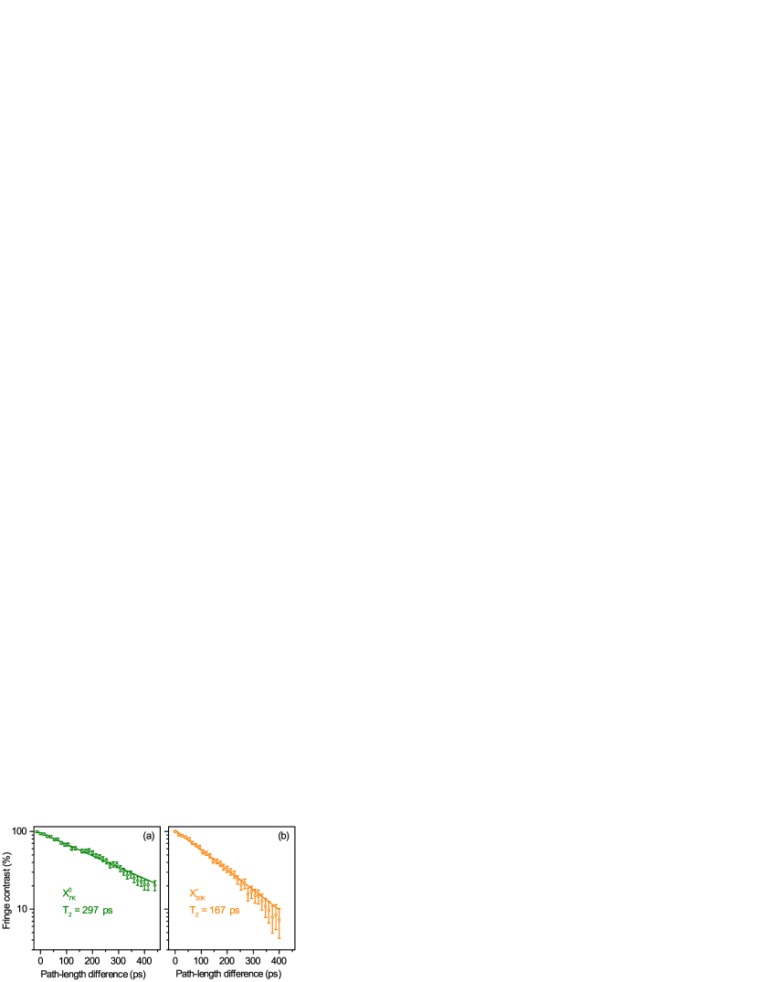
Figure 7: First-order correlation measurements obtained with a fiber-based Michelson-interferometer. Solid lines represent exponential fits to the data for (a) X⁰ at 7 K and (b) X⁺ at 30 K under p-shell excitation at $\lambda=909\,$nm.

We determine the coherence time $T_{2}$ of the charged X⁺ and neutral X⁰ exciton state under p-shell excitation at $\lambda=910\,$nm from first-order autocorrelation-measurements $g^{(1)}(\tau)$. Spectrally filtered photons were coupled into a fiber-based Michelson-interferometer to obtain the fringe contrast as a function of the path-length difference. Fitting the data with an exponential decay yields a coherence time of $T_{2}=(291\pm 6)\,$ps for the X⁰ at 7 K and $T_{2}=(167\pm 3)\,$ps for X⁺ at 30 K as displayed in Fig. 7. In both cases the coherence time is significantly below the values of 692 ps and 431 ps for X${}^{0}_{7K}$ and X${}^{+}_{30K}$, respectively, obtained by fitting Eq. 3 of the maintext to the experimental data in Fig. 4 of the main text (cf. Table I in main text) and considering the limit $\delta t\rightarrow\infty$ ($\Gamma^{\prime}=\Gamma_{0}^{\prime}$).






Theory: In this section, we provide a more detailed derivation of the formula for the HOM visibility in Eq. 3 of the maintext. The derivation follows the method presented by Bylander et al. Bylander et al. (2003):

$$V(\delta t,\tau_{c},T)= 1-\frac{\Gamma^{\prime}_{0}(1-e^{-\left(\frac{\delta t}{\tau_{c}}\right)^{2}})+\gamma(T)}{\Gamma^{\prime}_{0}(1-e^{-\left(\frac{\delta t}{\tau_{c}}\right)^{2}})+\gamma(T)+\Gamma}=\frac{\Gamma}{\Gamma^{\prime}_{0}(1-e^{-\left(\frac{\delta t}{\tau_{c}}\right)^{2}})+\gamma(T)+\Gamma}\ .$$ (7)

Mainly three dephasing/relaxation processes are present in the experiment: the radiative dephasing $\Gamma$, the phonon-induced pure dephasing $\gamma$, and the dephasing due to spectral diffusion $\Gamma^{\prime}:=\Gamma_{0}^{\prime}(1-e^{-(\delta t/\tau_{c})^{2}})$.
 
The total Hamiltonian includes the classical excitation field, the quantized light field, and the QD. It reads:

$$H/\hbar= \left(\omega_{e}+F(t)\right)\sigma_{ee}+\Omega(t)\left(e^{-i\omega_{p}t}\sigma_{eg}+e^{+i\omega_{p}t}\sigma_{ge}\right)+\int_{0}^{\infty}d\omega\left(\omega\ c^{\dagger}_{\omega}c^{\phantom{\dagger}}_{\omega}+g_{\omega}\ c^{\dagger}_{\omega}\sigma_{ge}+g_{\omega}^{*}\sigma_{eg}c^{\phantom{\dagger}}_{\omega}\right)\ ,$$ (8)

where we approximated the QD as a two-level system with the ground $\left|g\right\rangle$ and excited state $\left|e\right\rangle$ and respective lowering and raising operators defined by $\sigma_{ij}:=\left|i\right\rangle\left\langle j\right|$. The transition energy between the excited and ground state is denoted by $\omega_{e}$, where we set the ground state energy to zero. To adress dephasing, we apply the commonly used phenomenological dephasing description by including a general stochastic force $F(t)$ (here not specified, see discussion in the paper). Further, we assume a classical light field with amplitude $\Omega(t)$ in resonance with the transition energy $\omega_{p}=\omega_{e}$ and a quantized light field with annihilation and creation operator $c^{\phantom{\dagger}}_{\omega},c^{\dagger}_{\omega}$ as well as a light-matter coupling strength $g_{\omega}$, which is assumed to depend only weakly on frequency $g_{\omega}\approx g$. In the following, we need to distinguish between the photons, which take the longer route to the final beam splitter to compensate for the earlier emission process, and those, which reach the beam splitter via the short route. We distinguish the photons of both channels with the labels: $\omega_{L}$ for long and $\omega_{S}$ for short, i.e. the photons are distinguishable via their spatial travelling direction until they superpose at the final beam splitter.

The Hamiltonian is applied to the total wave function, being restricted by the experiment to the two-photon subspace:

$$\left|\Psi(t)\right\rangle= c_{g}(t)\left|g\right\rangle+c_{e}(t)\left|e\right\rangle+\int d\omega_{L}\ c_{\omega_{L}}(t)\left|g,1_{\omega_{L}}\right\rangle+\int d\omega_{L}\ c^{e}_{\omega_{L}}(t)\left|e,1_{\omega_{L}}\right\rangle$$

$$\ +\iint d\omega_{L}d\omega_{S}\ c_{\omega_{S}\omega_{L}}(t)\left|g,1_{\omega_{L}},1_{\omega_{S}}\right\rangle\ ,$$ (9)

Here, we assume that the first emitted photon cannot interact with the QD a second time, i.e. after the first excitation and subsequent first photon emission. Therefore, a state, such as $\left|g,2_{\omega_{L}},0_{\omega_{S}}\right\rangle$ is not taken into account, provided that the excitation process is faster than the emission time scale. Switching into the interaction picture and assuming that the p-shell excitation is fast compared to any quantum optical emission dynamics, we start with an initial condition $c_{e}(0)=1$ and solve the Wigner-Weisskopf problem:

$$\partial_{t}c_{e}= -ig\int d\omega\ e^{-i(\omega-\omega_{e})t+i\phi(t)}c_{\omega}$$ (10)

$$\partial_{t}c_{\omega}= -i\ g\ e^{i(\omega-\omega_{e})t-i\phi(t)}c_{e}\ .$$ (11)

Integrating the latter equation formally and plug them into the first equation, one yields a simple relaxation dynamics for the excited state, and the corresponding photon wave package form:

$$\partial_{t}c_{e}= -g^{2}\pi c_{e}(t)\rightarrow c_{e}(t)=c_{e}(0)e^{-\Gamma t}$$ (12)

$$c_{\omega}(t)= -i\ g\ \int_{0}^{t}dt^{\prime}e^{i(\omega-\omega_{e})t^{\prime}-i\phi(t^{\prime})}c_{e}(0)e^{-\Gamma t^{\prime}}\ ,$$ (13)

using the abbreviation $\Gamma=g^{2}\pi$ and including the frequency shift into the resonance condition. Note, we restricted our analysis to a one-dimensional problem. This is in accordance to the experiment, where the fiber and the optical setup allow for such a treatment.
 
For the subsequent excitation pulse, we assume $|c_{e}(t)|^{2}\approx 0$, with $t>\delta t$ and $\delta t$ the temporal distance between the two excitation pulses. Since the first photon wave package cannot interact with the QD anymore, the wave function between the photonic and electronic part factorizes and the same calculation as before can be applied. The two-photon wave function reads:

$$\left|\Psi(t)\right\rangle= \left[-ig\ \int_{0}^{\infty}d\omega_{S}\int_{\delta t}^{t}dt_{S}e^{i(\omega_{S}-\omega_{e})t_{S}-i\phi_{\delta t}(t_{S})-\Gamma t_{S}}\ c^{\dagger}_{\omega_{S}}\left|0_{\omega_{S}}\right\rangle\right]$$

$$\otimes\left[-ig\ \int_{0}^{\infty}d\omega_{L}\int_{0}^{t}dt_{L}e^{i(\omega_{L}-\omega_{e})t_{L}-i\phi_{0}(t_{L})-\Gamma t_{L}}c^{\dagger}_{\omega_{L}}\left|0_{\omega_{L}}\right\rangle\right]\ .$$ (14)

Note, the difference in the lower limit of the integrals ($0,\delta t$) and in the integrated noise signals

$$\phi_{t_{1}}(t)= \int_{t_{1}}^{t}dt^{\prime}F(t^{\prime})\ .$$ (15)

Given this wave function, we can calculate the observables of the experiment, as discussed in the following.

The Hong-Ou-Mandel effect leads to a vanishing two-photon-correlation for a pair of indistinguishable photons as both photons travelling either via the transmission or reflection path through the beam splitter. The quantity of interest is this two-photon correlation g${}^{(2)}(t_{D},t_{D}+\tau)$ between photons measured during the time $t_{D}$ on detector $A$ and $B$ with a delay of $\tau$:

$$g^{(2)}(t_{D},t_{D}+\tau)= \frac{\left\langle\Psi(t)\right|E^{(-)}_{A}(t_{D})E^{(-)}_{B}(t_{D}+\tau)E^{(+)}_{B}(t_{D}+\tau)E^{(+)}_{A}(t_{D})\left|\Psi(t_{D})\right\rangle}{\left\langle\Psi(t)\right|E^{(-)}_{B}(t_{D}+\tau)E^{(+)}_{B}(t_{D}+\tau)\left|\Psi(t)\right\rangle\left\langle\Psi(t)\right|E^{(-)}_{A}(t_{D})E^{(+)}_{A}(t_{D})\left|\Psi(t)\right\rangle}\ .$$ (16)

The electric fields $E_{A}$ and $E_{B}$ are calculated via the incoming fields of the long and short fiber and the transmission and reflection coefficients:

$$E^{(\pm)}_{A}= \sqrt{T}E^{(\pm)}_{S}+\sqrt{R}E^{(\pm)}_{L}$$ (17)

$$E^{(\pm)}_{B}= \sqrt{T}E^{(\pm)}_{L}-\sqrt{R}E^{(\pm)}_{S}\ .$$ (18)

For the two-photon correlation, we need to calculate the ket:

$$E^{(+)}(t_{D}+\tau)_{B}E^{(+)}_{A}(t_{D})\left|\psi(t)\right\rangle= \left[TE^{(+)}_{S}(t_{D}+\tau)E^{(+)}_{L}(t_{D})-RE^{(+)}_{L}(t_{D}+\tau)E^{(+)}_{S}(t_{D})\right]\left|\psi(t)\right\rangle\ .$$

Here, we omitted all contributions, where two photons in the long or short channel are needed. Using the commutation relations $[c^{\phantom{\dagger}}_{\omega_{i}},c^{\dagger}_{\omega^{\prime}_{j}}]=\delta_{ij}\delta(\omega-\omega^{\prime})$, we can evaluate the ket further and yield:

$$E^{(+)}_{B}(t_{D}+\tau)E^{(+)}_{A}(t_{D})\left|\Psi(t)\right\rangle\$$

$$=[-ig]^{2}\iint d\omega_{2}d\omega_{1}\left(Te^{-i\omega_{2}(t_{D}+\tau)}e^{-i\omega_{1}t_{D}}-Re^{-i\omega_{1}(t_{D}+\tau)}e^{-i\omega_{2}t_{D}}\right)$$ (19)

$$\qquad\qquad\int_{0}^{t}dt^{\prime\prime}e^{i(\omega_{1}-\omega_{e})t^{\prime\prime}-i\phi(t^{\prime\prime})}e^{-\Gamma t^{\prime\prime}}\int_{T}^{t}dt^{\prime}e^{i(\omega_{2}-\omega_{e})t^{\prime}-i\phi_{T}(t^{\prime})}e^{-\Gamma t^{\prime}}\left|g,0,0\right\rangle\ .$$

Integrating over the frequencies and considering the long-time limit $t\rightarrow\infty$, we yield for the unnormalized two-photon correlation:

$$E^{(+)}_{B}(t_{D}+\tau)E^{(+)}_{A}(t_{D})\left|\Psi(t)\right\rangle\$$

$$=-g^{2}\pi^{2}\left[Te^{-i\phi(t_{D}+\tau)-i\phi_{\delta t}(t_{D})}-Re^{-i\phi_{\delta t}(t_{D}+\tau)-i\phi_{\delta t}(t_{D})}\right]e^{-i\omega_{e}(2t_{D}+\tau)-\Gamma(2t_{D}+\tau)}\left|g,0,0\right\rangle\ .$$ (20)

The unnormalized two-photon correlation $G^{(2)}(t,\tau)$ is the product of Eq. (20) and its conjugate:

$$G^{(2)}(t_{D},\tau)=g^{4}\pi^{4}e^{-\Gamma(2t_{D}+\tau)}\left[T^{2}+R^{2}-2RT\ \text{Re}\left[\left\langle e^{-i\phi(t_{D}+\tau)-i\phi_{\delta t}(t_{D})+i\phi_{\delta t}(t_{D}+\tau)+i\phi(t_{D})}\right\rangle\right]\right]\ ,$$ (21)

where we already wrote the statistical averaging into the formula by $\langle\cdot\rangle$.

At this point, we need to specify the noise correlations to evaluate this expression further. To evaluate the stochastic forces, we need to average via a Gaussian random number distribution $\left\langle\left\langle\cdot\right\rangle\right\rangle$, where all higher moments can be expressed by the second-order correlation Gardiner and Zoller (2004). Eq. (21) is still very general in terms of dephasing processes and can be evaluated for Markovian- and non-Markovian noise correlations. To include dephasing, we employ the working horse of the phenomenological dephasing description by including a general stochastic force $F(t)=P(t)+D(t)$ with a phonon-induced dephasing ($\delta$-correlated white noise) $P(t)$ and a spectral diffusion $D(t)$ component (colored noise), both shifting the transition energy of the QD. First, we assume that the phonon-induced dephasing and the dephasing stemming from the spectral diffusion in the material are independent of each other. Therefore, we can neglect correlations between $D(t)$ and $P(t)$ in the cumulant expansion. Here, we restrict our investigation to the zero-phonon line broadening mechanism Borri et al. (2001). A possible source for such a dephasing mechanism is the quadratic interaction with longitudinal acoustical phonons, which gives rise to a temperature-dependent broadening Förstner et al. (2003); Muljarov and Zimmermann (2004). We also neglect contributions from highly non-Markovian phonon-sidebands, which also effect the indistiguishability, e.g. in cQED setups Kaer et al. (2013a, b), and described often with the independent Boson model Stock et al. (2011) or Feynman path integrals Vagov et al. (2011). Here, we employ the simplest possible model for such a dephasing by assuming a Markovian process $\delta-$correlated in time, i.e. as white noise Gardiner and Zoller (2004); Santori et al. (2009).

$$\left\langle\left\langle\phi^{P}_{t_{1}}(t_{2})\phi^{P}_{t_{1}}(t_{4})\right\rangle\right\rangle=\int_{t_{1}}^{t_{2}}dt\int_{t_{3}}^{t_{4}}dt^{\prime}\left\langle P(t)P(t^{\prime})\right\rangle= \gamma\left(\text{min}[t_{2},t_{4}]-\text{max}[t_{1},t_{3}]\right)\ .$$ (22)

The phonon-induced dephasing is highly temperature-dependent and limits the absolute value of the indistinguishability, independent of the temporal distance of the excitation pulses $\delta t$. In contrast to the phonon-induced dephasing, the spectral diffusion includes a strong dependence on the pulse distance. We include this dependence as a finite memory-effect with specific correlation time $\tau_{c}$:

$$\left\langle\left\langle\phi^{D}_{t_{1}}(t_{2})\phi^{D}_{t_{3}}(t_{4})\right\rangle\right\rangle= \int_{t_{1}}^{t_{2}}dt\int_{t_{3}}^{t_{4}}dt^{\prime}\left\langle D(t)D(t^{\prime})\right\rangle=\Gamma^{\prime}_{0}\ e^{-\frac{(t_{1}-t_{3})^{2}}{\tau_{c}^{2}}}\left(\text{min}[t_{2},t_{4}]-\text{max}[t_{1},t_{3}]\right)\ .$$ (23)

These kinds of noise correlations stem from a non-Markovian low-frequency noise Galperin et al. (2006); Laikhtman (1985); Eberly et al. (1984) and show plateau-like behavior for temporal pulse distances sufficiently short in comparison to the memory depth, i.e. for $\delta t\ll\tau_{c}$ the effect of spectral diffusion becomes negligible and only the phonon-induced dephasing limits the absolute value of the visibility.
 
The unnormalized two-photon correlation then reads:

$$G^{(2)}(t_{D},\tau)= g^{4}\pi^{4}e^{-2\Gamma t_{D}}\left[T^{2}e^{-\Gamma\tau}+R^{2}e^{-\Gamma\tau}-2RT\ e^{-(\gamma^{\prime}+\Gamma)\tau}\right],$$ (24)

$$\gamma^{\prime}= \Gamma^{\prime}_{0}\left(1-\exp[-(\delta t/\tau_{c})^{2}]\right)+\gamma\ ,$$ (25)

with $\delta t$ the temporal pulse distance, $\Gamma^{\prime}_{0}$ the spectral diffusion constant, and $\gamma$ the phonon-induced dephasing. As the measured quantity is the time-integrated photon correlation, integrating with respect to $t_{D}$ and $\tau$ yields, using $R+T=1$:

$$\bar{g}^{(2)}=\frac{2}{\pi^{2}(T^{2}+R^{2})}\int_{0}^{\infty}\int_{0}^{\infty}\text{d}\tau\text{d}t\ G^{(2)}(t,\tau)=1-\frac{2RT}{1-2RT}\frac{\Gamma}{\gamma^{\prime}+\Gamma}\ .$$ (26)

The visibility can be expressed via the normalized two-photon-correlation

$$V= 1-\bar{g}^{(2)}=\frac{2RT}{1-2RT}\left[1-\frac{\gamma^{\prime}}{\gamma^{\prime}+\Gamma}\right]\ .$$ (27)

With these equations at hand, we are now able explicitly formulate the dependence of the visibility on the pulse separation $\delta t$, the pure dephasing $\gamma$, and the diffusion constant $\Gamma^{\prime}$:

$$V= \frac{\Gamma}{\Gamma^{\prime}_{0}(1-\exp[-(\delta t/\tau_{c})^{2}])+\gamma(T)+\Gamma}\ ,$$ (28)

where a balanced beamsplitter ($T=R=1/2$) was assumed. Thus, for vanishing phonon-induced dephasing and spectral diffusion, the visibility is $1$, i.e. the photons are only Fourier-transform-limited and coalesce at the beamsplitter into a perfect coherent two-photon state. If the phonon-induced dephasing is stronger than other dephasing and relaxation processes $\gamma\gg\Gamma,\Gamma^{\prime}$, the visibility becomes small, which is typically seen in the high temperature limit. At low temperatures, the phonon-induced dephasing is small and the spectral diffusion with a finite-memory depth dictates the functional form of the visibility for different pulse distances.
 
To approximate the temperature dependence of the visibility, we employ the Markovian approximation for phonon-induced pure dephasing processes, where the dephasing is proportional to the square of the phonon number Carmichael (1999):

$$\gamma(T) =\gamma_{0}\ \bar{n}(T)\left[\bar{n}(T)+1\right]\ ,$$ (29)

where we have averaged over the frequency and approximated the expression via an effective phonon number depending on the temperature via the Bose-Einstein distribution for the effective phonon mode. The following formula is employed to underline the experimentally observed behavior qualitatively:

$$\bar{n}(T)= \left[\exp\left[\frac{\alpha}{T}\right]-1\right]^{-1}\ .$$ (30)

To fit the curve in Fig. 5 (d) in the maintext, we adjust the parameters $\gamma_{0}$ and $\alpha$. For illustrating purposes, we normalized the other dephasing contributions to one:

$$V(T)= \frac{\Gamma}{\Gamma^{\prime}_{0}(1-\exp[-(\delta t/\tau_{c})^{2}])+\gamma(T)+\Gamma}\approx\frac{1}{1+\gamma_{0}\ \bar{n}(\alpha,T)\left[\bar{n}(\alpha,T)+1\right]}\ .$$ (31)

The fit presented in Fig. 5 of the maintext, according to this formula, was performed with $\alpha=\hbar\bar{\omega}/k_{B}=44\,$K and $\gamma_{0}=3.75$.

References

- Knill et al. (2001) E. Knill, R. Laflamme, and G. J. Milburn, Nature 409, 46 (2001).
- Kiraz et al. (2004) A. Kiraz, M. Atatüre, and A. Imamoğlu, Phys. Rev. A 69, 032305 (2004).
- Kok et al. (2007) P. Kok, W. J. Munro, K. Nemoto, T. C. Ralph, J. P. Dowling, and G. J. Milburn, Rev. Mod. Phys. 79, 135 (2007).
- Gisin and Thew (2007) N. Gisin and R. Thew, Nature Photon. 1, 165 (2007).
- Kimble (2008) H. J. Kimble, Nature 453, 1023 (2008).
- Michler et al. (2000) P. Michler, A. Kiraz, C. Becher, W. V. Schoenfeld, P. M. Petroff, L. Zhang, E. Hu, and A. Imamoğlu, Science 290, 2282 (2000).
- Santori et al. (2002) C. Santori, D. Fattal, J. Vučković, G. S. Solomon, and Y. Yamamoto, Nature 419, 594 (2002).
- Patel et al. (2008) R. B. Patel, A. J. Bennett, K. Cooper, P. Atkinson, C. A. Nicoll, D. A. Ritchie, and A. J. Shields, Phys. Rev. Lett. 100, 207405 (2008).
- Ates et al. (2009) S. Ates, S. M. Ulrich, A. Ulhaq, S. Reitzenstein, A. Loffler, S. Hofling, A. Forchel, and P. Michler, Nature Photon. 3, 724 (2009).
- Wei et al. (2014) Y.-J. Wei, Y.-M. He, M.-C. Chen, Y.-N. Hu, Y. He, D. Wu, C. Schneider, M. Kamp, S. Höfling, C.-Y. Lu, and J.-W. Pan, Nano Lett. 14, 6515 (2014).
- Santori et al. (2004) C. Santori, D. Fattal, J. Vuckovic, G. S. Solomon, and Y. Yamamoto, New J. Phys. 6, 89 (2004).
- Varoutsis et al. (2005) S. Varoutsis, S. Laurent, P. Kramper, A. Lemaître, I. Sagnes, I. Robert-Philip, and I. Abram, Physical Review B 72, 041303 (2005).
- Gazzano et al. (2013) O. Gazzano, S. Michaelis de Vasconcellos, C. Arnold, A. Nowak, E. Galopin, I. Sagnes, L. Lanco, A. Lemaître, and P. Senellart, Nat. Commun. 4, 1425 (2013).
- Gold et al. (2014) P. Gold, A. Thoma, S. Maier, S. Reitzenstein, C. Schneider, S. Höfling, and M. Kamp, Phys. Rev. B 89, 035313 (2014).
- Hong et al. (1987) C. K. Hong, Z. Y. Ou, and L. Mandel, Phys. Rev. Lett. 59, 2044 (1987).
- Bennett et al. (2005) A. J. Bennett, D. C. Unitt, A. J. Shields, P. Atkinson, and D. A. Ritchie, Opt. Express 13, 7772 (2005).
- Wolters et al. (2013) J. Wolters, N. Sadzak, A. W. Schell, T. Schröder, and O. Benson, Phys. Rev. Lett. 110, 027401 (2013).
- Stanley et al. (2014) M. J. Stanley, C. Matthiesen, J. Hansom, C. Le Gall, C. H. H. Schulte, E. Clarke, and M. Atatüre, Phys. Rev. B 90, 195305 (2014).
- Gschrey et al. (2013) M. Gschrey, F. Gericke, A. Schüßler, R. Schmidt, J.-H. Schulze, T. Heindel, S. Rodt, A. Strittmatter, and S. Reitzenstein, Appl. Phys. Lett. 102, 251113 (2013).
- Gschrey et al. (2015) M. Gschrey, A. Thoma, P. Schnauber, M. Seifried, R. Schmidt, B. Wohlfeil, L. Krüger, J. H. Schulze, T. Heindel, S. Burger, F. Schmidt, A. Strittmatter, S. Rodt, and S. Reitzenstein, Nat. Commun. 6, 7662 (2015).
- Schlehahn et al. (2015a) A. Schlehahn, L. Krüger, M. Gschrey, J.-H. Schulze, S. Rodt, A. Strittmatter, T. Heindel, and S. Reitzenstein, Rev. Sci. Instrum. 86, 013113 (2015a).
- Bylander et al. (2003) J. Bylander, I. Robert-Philip, and I. Abram, EPJ D 22, 295 (2003).
- Empedocles and Bawendi (1997) S. A. Empedocles and M. G. Bawendi, Science 278, 2114 (1997).
- Robinson and Goldberg (2000) H. D. Robinson and B. B. Goldberg, Phys. Rev. B 61, R5086 (2000).
- Türck et al. (2000) V. Türck, S. Rodt, O. Stier, R. Heitz, R. Engelhardt, U. W. Pohl, D. Bimberg, and R. Steingrüber, Phys. Rev. B 61, 9944 (2000).
- Sallen et al. (2010) G. Sallen, A. Tribu, T. Aichele, R. André, L. Besombes, C. Bougerol, M. Richard, S. Tatarenko, K. Kheng, and J.-P. Poizat, Nature Photon. 4, 696 (2010).
- Houel et al. (2012) J. Houel, A. V. Kuhlmann, L. Greuter, F. Xue, M. Poggio, B. D. Gerardot, P. A. Dalgarno, A. Badolato, P. M. Petroff, A. Ludwig, D. Reuter, A. D. Wieck, and R. J. Warburton, Phys. Rev. Lett. 108, 107401 (2012).
- Müller et al. (2014) M. Müller, S. Bounouar, K. D. Jöns, M. Gläßl, and P. Michler, Nature Photon. 8, 224 (2014).
- Galperin et al. (2006) Y. M. Galperin, B. L. Altshuler, J. Bergli, and D. V. Shantsev, Phys. Rev. Lett. 96, 097009 (2006).
- Gardiner and Zoller (2004) C. Gardiner and P. Zoller, Quantum Noise: A Handbook of Markovian and Non-Markovian Quantum Stochastic Methods with Applications to Quantum Optics, Springer Series in Synergetics (Springer, 2004).
- Laikhtman (1985) B. D. Laikhtman, Phys. Rev. B 31, 490 (1985).
- Eberly et al. (1984) J. H. Eberly, K. Wódkiewicz, and B. W. Shore, Phys. Rev. A 30, 2381 (1984).
- Carmichael (1999) H. Carmichael, Statistical Methods in Quantum Optics 1 - Master Equation and Fokker-Planck Equations (Springer, 1999).
- Patel et al. (2010) R. B. Patel, A. J. Bennett, I. Farrer, C. A. Nicoll, D. A. Ritchie, and A. J. Shields, Nature Photon. 4, 632 (2010).
- Flagg et al. (2010) E. B. Flagg, A. Muller, S. V. Polyakov, A. Ling, A. Migdall, and G. S. Solomon, Phys. Rev. Lett. 104, 137401 (2010).
- Bernien et al. (2012) H. Bernien, L. Childress, L. Robledo, M. Markham, D. Twitchen, and R. Hanson, Phys. Rev. Lett. 108, 043604 (2012).
- Ma et al. (2011) X.-s. Ma, S. Zotter, J. Kofler, T. Jennewein, and A. Zeilinger, Phys. Rev. A 83, 043814 (2011).
- Schlehahn et al. (2015b) A. Schlehahn, M. Gaafar, M. Vaupel, M. Gschrey, P. Schnauber, J.-H. Schulze, S. Rodt, A. Strittmatter, W. Stolz, A. Rahimi-Iman, T. Heindel, M. Koch, and S. Reitzenstein, Appl. Phys. Lett. 107, 041105 (2015b).
- Borri et al. (2001) P. Borri, W. Langbein, S. Schneider, U. Woggon, R. L. Sellin, D. Ouyang, and D. Bimberg, Phys. Rev. Lett. 87, 157401 (2001).
- Förstner et al. (2003) J. Förstner, C. Weber, J. Danckwerts, and A. Knorr, Phys. Status Solidi (b) 238, 419 (2003).
- Muljarov and Zimmermann (2004) E. A. Muljarov and R. Zimmermann, Phys. Rev. Lett. 93, 237401 (2004).
- Kaer et al. (2013a) P. Kaer, N. Gregersen, and J. Mork, New J. Phys. 15, 035027 (2013a).
- Kaer et al. (2013b) P. Kaer, P. Lodahl, A.-P. Jauho, and J. Mork, Phys. Rev. B 87, 081308 (2013b).
- Stock et al. (2011) E. Stock, M.-R. Dachner, T. Warming, A. Schliwa, A. Lochmann, A. Hoffmann, A. I. Toropov, A. K. Bakarov, I. A. Derebezov, M. Richter, V. A. Haisler, A. Knorr, and D. Bimberg, Phys. Rev. B 83, 041304 (2011).
- Vagov et al. (2011) A. Vagov, M. D. Croitoru, M. Glässl, V. M. Axt, and T. Kuhn, Phys. Rev. B 83, 094303 (2011).
- Santori et al. (2009) C. Santori, D. Fattal, K.-M. C. Fu, P. E. Barclay, and R. G. Beausoleil, New J. Phys. 11, 123009 (2009).