Sparse Representation of Multivariate Extremes with Applications to Anomaly Detection

Abstract

Capturing the dependence structure of multivariate extreme events is a major concern in many fields involving the management of risks stemming from multiple sources, e.g. portfolio monitoring, insurance, environmental risk management and anomaly detection. One convenient (nonparametric) characterization of extreme dependence in the framework of multivariate Extreme Value Theory (EVT) is the angular measure, which provides direct information about the probable ’directions’ of extremes, that is, the relative contribution of each feature/coordinate of the ‘largest’ observations. Modeling the angular measure in high dimensional problems is a major challenge for the multivariate analysis of rare events. The present paper proposes a novel methodology aiming at exhibiting a sparsity pattern within the dependence structure of extremes. This is achieved by estimating the amount of mass spread by the angular measure on representative sets of directions, corresponding to specific sub-cones of $\mathbb{R}_{+}^{d}$. This dimension reduction technique paves the way towards scaling up existing multivariate EVT methods. Beyond a non-asymptotic study providing a theoretical validity framework for our method, we propose as a direct application a –first– Anomaly Detection algorithm based on multivariate EVT. This algorithm builds a sparse ‘normal profile’ of extreme behaviours, to be confronted with new (possibly abnormal) extreme observations. Illustrative experimental results provide strong empirical evidence of the relevance of our approach.

1 Introduction

1.1 Context: multivariate extreme values in large dimension

Extreme Value Theory (EVT in abbreviated form) provides a theoretical basis for modeling the tails of probability distributions. In many applied fields where rare events may have a disastrous impact, such as finance, insurance, climate, environmental risk management, network monitoring (Finkenstadt and Rootzén (2003); Smith (2003)) or anomaly detection (Clifton et al. (2011); Lee and Roberts (2008)), the information carried by extremes is crucial. In a multivariate context, the dependence structure of the joint tail is of particular interest, as it gives access e.g. to probabilities of a joint excess above high thresholds or to multivariate quantile regions. Also, the distributional structure of extremes indicates which components of a multivariate quantity may be simultaneously large while the others stay small, which is a valuable piece of information for multi-factor risk assessment or detection of anomalies among other –not abnormal– extreme data.

In a multivariate ‘Peak-Over-Threshold’ setting, realizations of a $d$ -dimensional random vector $\mathbf{Y}=(Y_{1},...,Y_{d})$ are observed and the goal pursued is to learn the conditional distribution of excesses, $\left[~{}\mathbf{Y}~{}|~{}\|\mathbf{Y}\|\geq r~{}\right]$, above some large threshold $r>0$. The dependence structure of such excesses is described via the distribution of the ‘directions’ formed by the most extreme observations, the so-called angular measure, hereafter denoted by $\Phi$. The latter is defined on the positive orthant of the $d-1$ dimensional hyper-sphere. To wit, for any region $A$ on the unit sphere (a set of ‘directions’), after suitable standardization of the data (see Section 2), $C\Phi(A)\simeq\mathbb{P}(\|\mathbf{Y}\|^{-1}\mathbf{Y}\in A~{}|~{}\|\mathbf{Y}\|>r)$, where $C$ is a normalizing constant. Some probability mass may be spread on any sub-sphere of dimension $k<d$, the $k$-faces of an hyper-cube if we use the infinity norm, which complexifies inference when $d$ is large. To fix ideas, the presence of $\Phi$-mass on a sub-sphere of the type $\{\max_{1\leq i\leq k}x_{i}=1~{};~{}x_{i}>0\;(i\leq k)~{};~{}x_{k+1}=\ldots=x_{d}=0\}$ indicates that the components $Y_{1},\ldots,Y_{k}$ may simultaneously be large, while the others are small. An extensive exposition of this multivariate extreme setting may be found e.g. in Resnick (1987), Beirlant et al. (2004).

Parametric or semi-parametric modeling and estimation of the structure of multivariate extremes is relatively well documented in the statistical literature, see e.g. Coles and Tawn (1991); Fougères et al. (2009); Cooley et al. (2010); Sabourin and Naveau (2012) and the references therein. In a non-parametric setting, there is also an abundant literature concerning consistency and asymptotic normality of estimators of functionals characterizing the extreme dependence structure, e.g. extreme value copulas or the stable tail dependence function (STDF), see Segers (2012), Drees and Huang (1998), Embrechts et al. (2000), Einmahl et al. (2012), de Haan and Ferreira (2006). In many applications, it is nevertheless more convenient to work with the angular measure itself, as the latter gives more direct information on the dependence structure and is able to reflect structural simplifying properties (e.g. sparsity as detailed below) which would not appear in copulas or in the STDF. However, non-parametric modeling of the angular measure faces major difficulties, stemming from the potentially complexe structure of the latter, especially in a high dimensional setting. Further, from a theoretical point of view, non-parametric estimation of the angular measure has only been studied in the two dimensional case, in Einmahl et al. (2001) and Einmahl and Segers (2009), in an asymptotic framework.

Scaling up multivariate EVT is a major challenge that one faces when confronted to high-dimensional learning tasks, since most multivariate extreme value models have been designed to handle moderate dimensional problems (say, of dimensionality $d\leq 10$). For larger dimensions, simplifying modeling choices are needed, stipulating e.g that only some pre-definite subgroups of components may be concomitantly extremes, or, on the contrary, that all of them must be (see e.g. Stephenson (2009) or Sabourin and Naveau (2012)). This curse of dimensionality can be explained, in the context of extreme values analysis, by the relative scarcity of extreme data, the computational complexity of the estimation procedure and, in the parametric case, by the fact that the dimension of the parameter space usually grows with that of the sample space. This calls for dimensionality reduction devices adapted to multivariate extreme values.

In a wide range of situations, one may expect the occurrence of two phenomena:

1- Only a ‘small’ number of groups of components may be concomitantly extreme, so that only a ‘small’ number of hyper-cubes (those corresponding to these subsets of indexes precisely) have non zero mass (‘small’ is relative to the total number of groups $2^{d}$).

2- Each of these groups contains a limited number of coordinates (compared to the original dimensionality), so that the corresponding hyper-cubes with non zero mass have small dimension compared to $d$.

The main purpose of this paper is to introduce a data-driven methodology for identifying such faces, so as to reduce the dimensionality of the problem and thus to learn a sparse representation of extreme behaviors. In case hypothesis 2- is not fulfilled, such a sparse ‘profile’ can still be learned, but looses the low dimensional property of its supporting hyper-cubes.

One major issue is that real data generally do not concentrate on sub-spaces of zero Lebesgue measure. This is circumvented by setting to zero any coordinate less than a threshold $\epsilon>0$, so that the corresponding ‘angle’ is assigned to a lower-dimensional face.

The theoretical results stated in this paper build on the work of Goix et al. (2015), where non-asymptotic bounds related to the statistical performance of a non-parametric estimator of the STDF, another functional measure of the dependence structure of extremes, are established. However, even in the case of a sparse angular measure, the support of the STDF would not be so, since the latter functional is an integrated version of the former (see (2.7), Section 2). Also, in many applications, it is more convenient to work with the angular measure. Indeed, it provides direct information about the probable ‘directions’ of extremes, that is, the relative contribution of each components of the ‘largest’ observations (where ‘large’ may be understood e.g. in the sense of the infinity norm on the input space). We emphasize again that estimating these ‘probable relative contributions’ is a major concern in many fields involving the management of risks from multiple sources. To the best of our knowledge, non-parametric estimation of the angular measure has only been treated in the two dimensional case, in Einmahl et al. (2001) and Einmahl and Segers (2009), in an asymptotic framework.

Main contributions. The present paper extends the non-asymptotic bounds proved in Goix et al. (2015) to the angular measure of extremes, restricted to a well-chosen representative class of sets, corresponding to lower-dimensional regions of the space. The objective is to learn a representation of the angular measure, rough enough to control the variance in high dimension and accurate enough to gain information about the ’probable directions’ of extremes. This yields a –first– non-parametric estimate of the angular measure in any dimension, restricted to a class of sub-cones, with a non asymptotic bound on the error. The representation thus obtained is exploited to detect anomalies among extremes.

The proposed algorithm is based on dimensionality reduction. We believe that our method can also be used as a preprocessing stage, for dimensionality reduction purpose, before proceeding with a parametric or semi-parametric estimation which could benefit from the structural information issued in the first step. Such applications are beyond the scope of this paper and will be the subject of further research.

1.2 Application to Anomaly Detection

Anomaly Detection (AD in short, and depending of the application domain, outlier detection, novelty detection, deviation detection, exception mining) generally consists in assuming that the dataset under study contains a small number of anomalies, generated by distribution models that differ from that generating the vast majority of the data. This formulation motivates many statistical AD methods, based on the underlying assumption that anomalies occur in low probability regions of the data generating process. Here and hereafter, the term ‘normal data’ does not refer to Gaussian distributed data, but to not abnormal ones, i.e. data belonging to the above mentioned majority. Classical parametric techniques, like those developed in Barnett and Lewis (1994) or in Eskin (2000), assume that the normal data are generated by a distribution belonging to some specific, known in advance parametric model. The most popular non-parametric approaches include algorithms based on density (level set) estimation (see e.g. Schölkopf et al. (2001), Scott and Nowak (2006) or Breunig et al. (1999)), on dimensionality reduction (cf Shyu et al. (2003), Aggarwal and Yu (2001)) or on decision trees (Liu et al. (2008)). One may refer to Hodge and Austin (2004), Chandola et al. (2009), Patcha and Park (2007) and Markou and Singh (2003) for excellent overviews of current research on Anomaly Detection, ad-hoc techniques being far too numerous to be listed here in an exhaustive manner. The framework we develop in this paper is non-parametric and lies at the intersection of support estimation, density estimation and dimensionality reduction: it consists in learning from training data the support of a distribution, that can be decomposed into sub-cones, hopefully of low dimension each and to which some mass is assigned, according to empirical versions of probability measures on extreme regions.

EVT has been intensively used in AD in the one-dimensional situation, see for instance Roberts (1999), Roberts (2000), Clifton et al. (2011), Clifton et al. (2008), Lee and Roberts (2008). In the multivariate setup, however, there is –to the best of our knowledge– no anomaly detection method relying on multivariate EVT. Until now, the multidimensional case has only been tackled by means of extreme value statistics based on univariate EVT. The major reason is the difficulty to scale up existing multivariate EVT models with the dimensionality. In the present paper we bridge the gap between the practice of AD and multivariate EVT by proposing a method which is able to learn a sparse ‘normal profile’ of multivariate extremes and, as such, may be implemented to improve the accuracy of any usual AD algorithm. Experimental results show that this method significantly improves the performance in extreme regions, as the risk is taken not to uniformly predict as abnormal the most extremal observations, but to learn their dependence structure. These improvements may typically be useful in applications where the cost of false positive errors (i.e. false alarms) is very high (e.g. predictive maintenance in aeronautics).

The structure of the paper is as follows. The whys and wherefores of multivariate EVT are explained in the following Section 2. A non-parametric estimator of the subfaces’ mass is introduced in Section 3, the accuracy of which is investigated by establishing finite sample error bounds relying on VC inequalities tailored to low probability regions. An application to Anomaly Detection is proposed in Section 4, where some background on AD is provided, followed by a novel AD algorithm which relies on the above mentioned non-parametric estimator. Experiments on both simulated and real data are performed in Section 5. Technical details are deferred to the Appendix section.

2 Multivariate EVT Framework and Problem Statement

Extreme Value Theory (EVT) develops models for learning the unusual rather than the usual, in order to provide a reasonable assessment of the probability of occurrence of rare events. Such models are widely used in fields involving risk management such as Finance, Insurance, Operation Research, Telecommunication or Environmental Sciences for instance. For clarity, we start off with recalling some key notions pertaining to (multivariate) EVT, that shall be involved in the formulation of the problem next stated and in its subsequent analysis.

2.1 Notations

Throughout the paper, bold symbols refer to multivariate quantities, and for $m\in\mathbb{R}\cup\{\infty\}$, $\mathbf{m}$ denotes the vector $(m,\ldots,m)$. Also, comparison operators between two vectors (or between a vector and a real number) are understood component-wise, i.e.  ‘$\mathbf{x}\leq\mathbf{z}$’ means ‘$x_{j}\leq z_{j}$ for all $1\leq j\leq d$’ and for any real number $T$, ‘$\mathbf{x}\leq T$’ means ‘$x_{j}\leq T$ for all $1\leq j\leq d$’. We denote by $\lfloor u\rfloor$ the integer part of any real number $u$, by $u_{+}=\max(0,\;u)$ its positive part and by $\delta_{\mathbf{a}}$ the Dirac mass at any point $\mathbf{a}\in\mathbb{R}^{d}$. For uni-dimensional random variables $Y_{1},\ldots,Y_{n}$, $Y_{(1)}\leq\ldots\leq Y_{(n)}$ denote their order statistics.

2.2 Background on (multivariate) Extreme Value Theory

In the univariate case, EVT essentially consists in modeling the distribution of the maxima (resp. the upper tail of the r.v. under study) as a generalized extreme value distribution, namely an element of the Gumbel, Fréchet or Weibull parametric families (resp. by a generalized Pareto distribution). It plays a crucial role in risk monitoring: consider the $(1-p)^{th}$ quantile of the distribution $F$ of a r.v. $X$, for a given exceedance probability $p$, that is $x_{p}=\inf\{x\in\mathbb{R},~{}\mathbb{P}(X>x)\leq p\}$. For moderate values of $p$, a natural empirical estimate is $x_{p,n}=\inf\{x\in\mathbb{R},~{}1/n\sum_{i=1}^{n}\mathds{1}_{\{X_{i}>x\}}\leq p\}$. However, if $p$ is very small, the finite sample $X_{1},\;\ldots,X_{n}$ carries insufficient information and the empirical quantile $x_{p,n}$ becomes unreliable. That is where EVT comes into play by providing parametric estimates of large quantiles: whereas statistical inference often involves sample means and the Central Limit Theorem, EVT handles phenomena whose behavior is not ruled by an ‘averaging effect’. The focus is on the sample maximum rather than the mean. The primal assumption is the existence of two sequences $\{a_{n},n\geq 1\}$ and $\{b_{n},n\geq 1\}$, the $a_{n}$’s being positive, and a non-degenerate distribution function $G$ such that

$$\lim_{n\to\infty}n~{}\mathbb{P}\left(\frac{X-b_{n}}{a_{n}}~{}\geq~{}x\right)=-\log G(x)$$ (2.1)

for all continuity points $x\in\mathbb{R}$ of $G$. If this assumption is fulfilled – it is the case for most textbook distributions – then $F$ is said to lie in the domain of attraction of $G$: $F\in DA(G)$. The tail behavior of $F$ is then essentially characterized by $G$, which is proved to be – up to re-scaling – of the type $G(x)=\exp(-(1+\gamma x)^{-1/\gamma})$ for $1+\gamma x>0$, $\gamma\in\mathbb{R}$, setting by convention $(1+\gamma x)^{-1/\gamma}=e^{-x}$ for $\gamma=0$. The sign of $\gamma$ controls the shape of the tail and various estimators of the re-scaling sequence and of the shape index $\gamma$ as well have been studied in great detail, see e.g. Dekkers et al. (1989), Einmahl et al. (2009), Hill (1975), Smith (1987), Beirlant et al. (1996).

Extensions to the multivariate setting are well understood from a probabilistic point of view, but far from obvious from a statistical perspective. Indeed, the tail dependence structure, ruling the possible simultaneous occurrence of large observations in several directions, has no finite-dimensional parametrization.

The analogue of (2.1) for a $d$-dimensional r.v.$\mathbf{X}=(X^{1},\;\ldots,\;X^{d})$ with distribution $\mathbf{F}(\mathbf{x}):=\mathbb{P}(X_{1}\leq x_{1},\ldots,X_{d}\leq x_{d})$, namely $\mathbf{F}\in\textbf{DA}(\mathbf{G})$ stipulates the existence of two sequences $\{\mathbf{a}_{n},n\geq 1\}$ and $\{\mathbf{b}_{n},n\geq 1\}$ in $\mathbb{R}^{d}$, the $\mathbf{a}_{n}$’s being positive, and a non-degenerate distribution function $\mathbf{G}$ such that

$$\lim_{n\to\infty}n~{}\mathbb{P}\left(\frac{X^{1}-b_{n}^{1}}{a_{n}^{1}}~{}\geq~{}x_{1}\text{~{}or~{}}\ldots\text{~{}or~{}}\frac{X^{d}-b_{n}^{d}}{a_{n}^{d}}~{}\geq~{}x_{d}\right)=-\log\mathbf{G}(\mathbf{x})$$ (2.2)

for all continuity points $\mathbf{x}\in\mathbb{R}^{d}$ of $\mathbf{G}$. This clearly implies that the margins $G_{1}(x_{1}),\ldots,G_{d}(x_{d})$ are univariate extreme value distributions, namely of the type $G_{j}(x)=\exp(-(1+\gamma_{j}x)^{-1/\gamma_{j}})$. Also, denoting by $F_{1},\;\ldots,\;F_{d}$ the marginal distributions of $\mathbf{F}$, Assumption (2.2) implies marginal convergence: $F_{i}\in DA(G_{i})$ for $i=1,\;\ldots,\;n$. To understand the structure of the limit $\mathbf{G}$ and dispose of the unknown sequences $(\mathbf{a}_{n},\mathbf{b}_{n})$ (which are entirely determined by the marginal distributions $F_{j}$’s), it is convenient to work with marginally standardized variables, that is, to separate the margins from the dependence structure in the description of the joint distribution of $\mathbf{X}$. Consider the standardized variables $V^{j}=1/(1-F_{j}(X^{j}))$ and $\mathbf{V}=(V^{1},\;\ldots,\;V^{d})$. In fact (see Proposition 5.10 in Resnick (1987)), Assumption (2.2) is equivalent to marginal convergences $F_{j}\in DA(G_{j})$ as in (2.1), together with standard multivariate regular variation of $\mathbf{V}$’s distribution, which means existence of a limit measure $\mu$ on $[0,\infty]^{d}\setminus\{\mathbf{0}\}$ such that

$$n~{}\mathbb{P}\left(\frac{V^{1}}{n}~{}\geq~{}v_{1}\text{~{}or~{}}\cdots\text{~{}or~{}}\frac{V^{d}}{n}~{}\geq~{}v_{d}\right)\xrightarrow[n\to\infty]{}\mu\left([\mathbf{0},\mathbf{v}]^{c}\right),$$ (2.3)

where $[\mathbf{0},\mathbf{v}]:=[0,\;v_{1}]\times\cdots\times[0,\;v_{d}]$. Thus, the variable $\mathbf{V}$ satisfies (2.2) with $\mathbf{a}_{n}=\mathbf{n}=(n,\;\ldots,\;n)$, $\mathbf{b}_{n}=\mathbf{0}=(0,\;\ldots,\;0)$. The dependence structure of the limit $\mathbf{G}$ in (2.2) can be expressed by means of the so-termed exponent measure $\mu$:

$$-\log\mathbf{G}(\mathbf{x})=\mu\left(\left[\mathbf{0},\left(\frac{-1}{\log G_{1}(x_{1})},\dots,\frac{-1}{\log G_{d}(x_{d})}\right)\right]^{c}\right).$$

The latter is finite on sets bounded away from $\mathbf{0}$ and has the homogeneity property : $\mu(t\,\cdot\,)=t^{-1}\mu(\,\cdot\,)$. Observe in addition that, due to the standardization chosen (with ‘nearly’ Pareto margins), the support of $\mu$ is included in $[\mathbf{0},\;\mathbf{1}]^{c}$. To wit, the measure $\mu$ should be viewed, up to a a normalizing factor, as the asymptotic distribution of $\mathbf{V}$ in extreme regions. For any borelian subset $A$ bounded away from $\mathbf{0}$ on which $\mu$ is continuous, we have

$$t~{}\mathbb{P}\left(\mathbf{V}\in tA\right)\xrightarrow[t\to\infty]{}\mu(A).$$ (2.4)

Using the homogeneity property $\mu(t\,\cdot\,)=t^{-1}\mu(\,\cdot\,)$, one may show that $\mu$ can be decomposed into a radial component and an angular component $\Phi$, which are independent from each other (see e.g. de Haan and Resnick (1977)). Indeed, for all $\mathbf{v}=(v_{1},...,v_{d})\in\mathbb{R}^{d}$, set

$$\left\{\begin{aligned} R(\mathbf{v})&:=\|\mathbf{v}\|_{\infty}~{}=~{}\max_{i=1}^{d}v_{i},\\ \Theta(\mathbf{v})&:=\left(\frac{v_{1}}{R(\mathbf{v})},...,\frac{v_{d}}{R(\mathbf{v})}\right)\in S_{\infty}^{d-1},\end{aligned}\right.$$ (2.5)

where $S_{\infty}^{d-1}$ is the positive orthant of the unit sphere in $\mathbb{R}^{d}$ for the infinity norm. Define the spectral measure (also called angular measure) by $\Phi(B)=\mu(\{\mathbf{v}~{}:~{}R(\mathbf{v})>1,\Theta(\mathbf{v})\in B\})$. Then, for every $B\subset S_{\infty}^{d-1}$,

$$\mu\{\mathbf{v}~{}:~{}R(\mathbf{v})>z,\Theta(\mathbf{v})\in B\}=z^{-1}\Phi(B)~{}.$$ (2.6)

In a nutshell, there is a one-to-one correspondence between the exponent measure $\mu$ and the angular measure $\Phi$, both of them can be used to characterize the asymptotic tail dependence of the distribution $\mathbf{F}$ (as soon as the margins $F_{j}$ are known), since

$$\mu\big{(}[\mathbf{0},\mathbf{x}^{-1}]^{c}\big{)}=\int_{\boldsymbol{\theta}\in S_{\infty}^{d-1}}\max_{j}{\boldsymbol{\theta}_{j}x_{j}}\;\mathrm{d}\Phi(\boldsymbol{\theta}),$$ (2.7)

this equality being obtained from the change of variable (2.5) , see e.g. Proposition 5.11 in Resnick (1987). Recall that here and beyond, operators on vectors are understood component-wise, so that $\mathbf{x}^{-1}=(x_{1}^{-1},\ldots,x_{d}^{{}_{1}})$. The angular measure can be seen as the asymptotic conditional distribution of the ‘angle’ $\Theta$ given that the radius $R$ is large, up to the normalizing constant $\Phi(S_{\infty}^{d-1})$. Indeed, dropping the dependence on $\mathbf{V}$ for convenience, we have for any continuity set $A$ of $\Phi$,

$$\mathbb{P}(\Theta\in A~{}|~{}R>r) =\frac{r\mathbb{P}(\Theta\in A,R>r)}{r\mathbb{P}(R>r)} \xrightarrow[r\to\infty]{}\frac{\Phi(A)}{\Phi(S_{\infty}^{d-1})}.$$ (2.8)

The choice of the marginal standardization is somewhat arbitrary and alternative standardizations lead to different limits. Another common choice consists in considering ‘nearly uniform’ variables (namely, uniform variables when the margins are continuous): defining $\mathbf{U}$ by $U^{j}=1-F_{j}(X^{j})$ for $j\in\{1,\ldots,d\}$, Condition (2.3) is equivalent to each of the following conditions:

• $\mathbf{U}$ has ‘inverse multivariate regular variation’ with limit measure $\Lambda(\,\cdot\,)$ $:=\mu((\,\cdot\,)^{-1})$, namely, for every measurable set $A$ bounded away from $+\boldsymbol{\infty}$ which is a continuity set of $\Lambda$,

  $$t~{}\mathbb{P}\left(\mathbf{U}\in t^{-1}A\right)\xrightarrow[t\to\infty]{}\Lambda(A)=\mu(A^{-1}),$$ (2.9)

  where $A^{-1}=\{\mathbf{u}\in\mathbb{R}^{d}_{+}~{}:~{}(u_{1}^{-1},\ldots,u_{d}^{-1})\in A\}$. The limit measure $\Lambda$ is finite on sets bounded away from $\{+\boldsymbol{\infty}\}$.

• The stable tail dependence function (STDF) defined for $\mathbf{x}\in[\mathbf{0},\boldsymbol{\infty}],\mathbf{x}\neq\boldsymbol{\infty}$ by

  $$l(\mathbf{x})=\lim_{t\to 0}t^{-1}\mathbb{P}\left(U^{1}\leq t\,x_{1}~{}\text{or}~{}\ldots~{}\text{or}~{}U^{d}\leq t\,x_{d}\right)=\mu\left([\mathbf{0},\mathbf{x}^{-1}]^{c}\right)$$ (2.10)

  exists.

2.3 Statement of the Statistical Problem

The focus of this work is on the dependence structure in extreme regions of a random vector $\mathbf{X}$ in a multivariate domain of attraction (see (2.1)). This asymptotic dependence is fully described by the exponent measure $\mu$, or equivalently by the spectral measure $\Phi$. The goal of this paper is to infer a meaningful (possibly sparse) summary of the latter. As shall be seen below, since the support of $\mu$ can be naturally partitioned in a specific and interpretable manner, this boils down to accurately recovering the mass spread on each element of the partition. In order to formulate this approach rigorously, additional definitions are required.

Truncated cones. For any non empty subset of features $\alpha\subset\{1,\;\ldots,\;d\}$, consider the truncated cone (see Fig. 1)

$$\mathcal{C}_{\alpha}=\{\mathbf{v}\geq 0,~{}\|\mathbf{v}\|_{\infty}\geq 1,~{}v_{j}>0~{}\text{ for }j\in\alpha,~{}v_{j}=0~{}\text{ for }j\notin\alpha\}.$$ (2.11)

The corresponding subset of the sphere is

$$\Omega_{\alpha}=\{\mathbf{x}\in S_{\infty}^{d-1}:x_{i}>0\text{ for }i\in\alpha~{},~{}x_{i}=0\text{ for }i\notin\alpha\}=S_{\infty}^{d-1}\cap{\mathcal{C}}_{\alpha},$$

and we clearly have $\mu(\mathcal{C}_{\alpha})=\Phi(\Omega_{\alpha})$ for any $\emptyset\neq\alpha\subset\{1,\;\ldots,\;d\}$. The collection $\{\mathcal{C}_{\alpha}:\;\emptyset\neq\alpha\subset\{1,\;\ldots,\;d\}\}$ forming a partition of the truncated positive orthant $\mathbb{R}_{+}^{d}\setminus[\mathbf{0},\mathbf{1}]$, one may naturally decompose the exponent measure as

$$\mu=\sum_{\emptyset\neq\alpha\subset\{1,\ldots,d\}}\mu_{\alpha},$$ (2.12)

where each component $\mu_{\alpha}$ is concentrated on the untruncated cone corresponding to ${\cal C_{\alpha}}$. Similarly, the $\Omega_{\alpha}$’s forming a partition of $S_{\infty}^{d-1}$, we have

$$\Phi~{}=~{}\sum_{\emptyset\neq\alpha\subset\{1,\ldots,d\}}\Phi_{\alpha}~{},$$

where $\Phi_{\alpha}$ denotes the restriction of $\Phi$ to ${\Omega}_{\alpha}$ for all $\emptyset\neq\alpha\subset\{1,\;\ldots,\;d\}$. The fact that mass is spread on $\mathcal{C}_{\alpha}$ indicates that conditioned upon the event ‘$R(\mathbf{V})$ is large’ (i.e. an excess of a large radial threshold), the components $V^{j}(j\in\alpha)$ may be simultaneously large while the other $V^{j}$’s $(j\notin\alpha)$ are small, with positive probability. Each index subset $\alpha$ thus defines a specific direction in the tail region.

However this interpretation should be handled with care, since for $\alpha\neq\{1,\ldots,d\}$, if $\mu(\mathcal{C}_{\alpha})>0$, then $\mathcal{C}_{\alpha}$ is not a continuity set of $\mu$ (it has empty interior), nor $\Omega_{\alpha}$ is a continuity set of $\Phi$. Thus, the quantity $t\mathbb{P}(\mathbf{V}\in t\mathcal{C}_{\alpha})$ does not necessarily converge to $\mu(\mathcal{C}_{\alpha})$ as $t\rightarrow+\infty$. Actually, if $\mathbf{F}$ is continuous, we have $\mathbb{P}(\mathbf{V}\in t\mathcal{C}_{\alpha})=0$ for any $t>0$. However, consider for $\epsilon\geq 0$ the $\epsilon$-thickened rectangles

$$R_{\alpha}^{\epsilon}~{}=\{\mathbf{v}\geq 0,~{}\|\mathbf{v}\|_{\infty}\geq 1,~{}v_{j}>\epsilon~{}\text{ for }j\in\alpha,~{}v_{j}\leq\epsilon~{}\text{ for }j\notin\alpha\},$$ (2.13)

Since the boundaries of the sets $R_{\alpha}^{\epsilon}$ are disjoint, only a countable number of them may be discontinuity sets of $\mu$. Hence, the threshold $\epsilon$ may be chosen arbitrarily small in such a way that $R_{\alpha}^{\epsilon}$ is a continuity set of $\mu$. The result stated below shows that nonzero mass on $\mathcal{C}_{\alpha}$ is the same as nonzero mass on $R_{\alpha}^{\epsilon}$ for $\epsilon$ arbitrarily small.

Figure 1: Truncated cones in 3D

Figure 2: Truncated $\epsilon$-rectangles in 2D

Lemma 1.

For any non empty index subset $\emptyset\neq\alpha\subset\{1,\ldots,d\}$, the exponent measure of $\mathcal{C}_{\alpha}$ is

$$\mu(\mathcal{C}_{\alpha})=\lim_{\epsilon\to 0}\mu(R_{\alpha}^{\epsilon}).$$

Proof.

First consider the case $\alpha=\{1,\ldots,d\}$. Then $R_{\alpha}^{\epsilon}$’s forms an increasing sequence of sets as $\epsilon$ decreases and $\mathcal{C}_{\alpha}=R_{\alpha}^{0}=\cup_{\epsilon>0,\epsilon\in\mathbb{Q}}~{}R_{\alpha}^{\epsilon}$. The result follows from the ‘continuity from below’ property of the measure $\mu$. Now, for $\epsilon\geq 0$ and $\alpha\subsetneq\{1,\;\ldots,\;d\}$, consider the sets

$$O_{\alpha}^{\epsilon} =\{\mathbf{x}\in\mathbb{R}_{+}^{d}~{}:\forall j\in\alpha:x_{j}>\epsilon\},$$

$$N_{\alpha}^{\epsilon} =\{\mathbf{x}\in\mathbb{R}_{+}^{d}~{}:\forall j\in\alpha:x_{j}>\epsilon,\exists j\notin\alpha:x_{j}>\epsilon\},$$

so that $N_{\alpha}^{\epsilon}\subset O_{\alpha}^{\epsilon}$ and $R_{\alpha}^{\epsilon}=O_{\alpha}^{\epsilon}\setminus N_{\alpha}^{\epsilon}$. Observe also that $\mathcal{C}_{\alpha}=O_{\alpha}^{0}\setminus N_{\alpha}^{0}$. Thus, $\mu(R_{\alpha}^{\epsilon})=\mu(O_{\alpha}^{\epsilon})-\mu(N_{\alpha}^{\epsilon})$, and $\mu(\mathcal{C}_{\alpha})=\mu(O_{\alpha}^{0})-\mu(N_{\alpha}^{0})$, so that it is sufficient to show that

$$\mu(N_{\alpha}^{0})=\lim_{\epsilon\to 0}\mu(N_{\alpha}^{\epsilon}),\quad\text{and}\quad\mu(O_{\alpha}^{0})=\lim_{\epsilon\to 0}\mu(O_{\alpha}^{\epsilon}).$$

Notice that the $N_{\alpha}^{\epsilon}$’s and the $O_{\alpha}^{\epsilon}$’s form two increasing sequences of sets (when $\epsilon$ decreases), and that $N_{\alpha}^{0}=\bigcup_{\epsilon>0,\epsilon\in\mathbb{Q}}N_{\alpha}^{\epsilon}$, $O_{\alpha}^{0}=\bigcup_{\epsilon>0,\epsilon\in\mathbb{Q}}O_{\alpha}^{\epsilon}$. This proves the desired result. ∎

We may now make precise the above heuristic interpretation of the quantities $\mu(\mathcal{C}_{\alpha})$: the vector $\mathcal{M}=\{\mu(\mathcal{C}_{\alpha}):\;\emptyset\neq\alpha\subset\{1,\;\ldots,\;d\}\}$ asymptotically describes the dependence structure of the extremal observations. Indeed, by Lemma 1, and the discussion above, $\epsilon$ may be chosen such that $R_{\alpha}^{\epsilon}$ is a continuity set of $\mu$, while $\mu(R_{\alpha}^{\epsilon})$ is arbitrarily close to $\mu(\mathcal{C}_{\alpha})$. Then, using the characterization (2.4) of $\mu$, the following asymptotic identity holds true:

$$\lim_{t\to\infty}t\mathbb{P}\left(\|\mathbf{V}\|_{\infty}\geq t,V^{j}>\epsilon t~{}~{}(j\in\alpha),V^{j}\leq\epsilon t~{}~{}(j\notin\alpha)\right) =\mu(R_{\alpha}^{\epsilon})$$

$$\simeq\mu(\mathcal{C}_{\alpha}).$$

Remark 1.

In terms of conditional probabilities, denoting $R=\|T(\mathbf{X})\|$, where $T$ is the standardization map $\mathbf{X}\mapsto\mathbf{V}$, we have

$$\mathbb{P}(T(\mathbf{X})\in rR_{\alpha}^{\epsilon}~{}|~{}R>r)=\frac{r\mathbb{P}(\mathbf{V}\in rR_{\alpha}^{\epsilon})}{r\mathbb{P}(\mathbf{V}\in r([\mathbf{0},\mathbf{1}]^{c})}\xrightarrow[r\to\infty]{}\frac{\mu(R_{\alpha}^{\epsilon})}{\mu([\mathbf{0},\mathbf{1}]^{c})},$$

as in (2.8). In other terms,

$$\mathbb{P}\left(V^{j}>\epsilon r~{}~{}(j\in\alpha),V^{j}\leq\epsilon r~{}~{}(j\notin\alpha)~{}\big{|}~{}\|\mathbf{V}\|_{\infty}\geq r\right) \xrightarrow[r\to\infty]{}C\mu(R_{\alpha}^{\epsilon})$$

$$~{}~{}~{}~{}~{}\simeq C\mu(\mathcal{C}_{\alpha}),$$

where $C=1/\Phi(S_{\infty}^{d-1})=1/\mu([\mathbf{0},\mathbf{1}]^{c})$. This clarifies the meaning of ‘large’ and ‘small’ in the heuristic explanation given above.

Problem statement. As explained above, our goal is to describe the dependence on extreme regions by investigating the structure of $\mu$ (or, equivalently, that of $\Phi$). More precisely, the aim is twofold. First, recover a rough approximation of the support of $\Phi$ based on the partition $\{\Omega_{\alpha},\alpha\subset\{1,\ldots,d\},\alpha\neq\emptyset\}$, that is, determine which $\Omega_{\alpha}$’s have nonzero mass, or equivalently, which $\mu_{\alpha}^{\prime}s$ (resp. $\Phi_{\alpha}$’s) are nonzero. This support estimation is potentially sparse (if a small number of $\Omega_{\alpha}$ have non-zero mass) and possibly low-dimensional (if the dimension of the sub-cones $\Omega_{\alpha}$ with non-zero mass is low). The second objective is to investigate how the exponent measure $\mu$ spreads its mass on the $\mathcal{C}_{\alpha}$’s, the theoretical quantity $\mu(\mathcal{C}_{\alpha})$ indicating to which extent extreme observations may occur in the ‘direction’ $\alpha$ for $\emptyset\neq\alpha\subset\{1,\;\ldots,\;d\}$. These two goals are achieved using empirical versions of the angular measure defined in Section 3.1, evaluated on the $\epsilon$-thickened rectangles $R_{\alpha}^{\epsilon}$. Formally, we wish to recover the $(2^{d}-1)$-dimensional unknown vector

$$\mathcal{M}=\{\mu(\mathcal{C}_{\alpha}):\;\emptyset\neq\alpha\subset\{1,\;\ldots,\;d\}\}$$ (2.14)

from $\mathbf{X}_{1},\;\ldots,\;\mathbf{X}_{n}\overset{i.i.d.}{\sim}\mathbf{F}$ and build an estimator $\widehat{\mathcal{M}}$ such that

$$||\widehat{\mathcal{M}}-\mathcal{M}||_{\infty}\;{=}\;\sup_{\emptyset\neq\alpha\subset\{1,\;\ldots,\;d\}}\;|\widehat{\mathcal{M}}(\alpha)-\mu(\mathcal{C}_{\alpha})|$$

is small with large probability. In view of Lemma 1, (biased) estimates of $\mathcal{M}$’s components are built from an empirical version of the exponent measure, evaluated on the $\epsilon$-thickened rectangles $R_{\alpha}^{\epsilon}$ (see Section 3.1 below). As a by-product, one obtains an estimate of the support of the limit measure $\mu$,

$$\bigcup_{\alpha:\;\widehat{\mathcal{M}}(\alpha)>0}\mathcal{C}_{\alpha}.$$

The results stated in the next section are non-asymptotic and sharp bounds are given by means of VC inequalities tailored to low probability regions.

2.4 Regularity Assumptions

Beyond the existence of the limit measure $\mu$ (i.e. multivariate regular variation of $\mathbf{V}$’s distribution, see (2.3)), and thus, existence of an angular measure $\Phi$ (see (2.6)), three additional assumptions are made, which are natural when estimation of the support of a distribution is considered.

Assumption 1.

The margins of $\mathbf{X}$ have continuous c.d.f., namely $F_{j},~{}1\leq j\leq d$ is continuous.

Assumption 1 is widely used in the context of non-parametric estimation of the dependence structure (see e.g. Einmahl and Segers (2009)): it ensures that the transformed variables $V^{j}=(1-F_{j}(X^{j}))^{-1}$ (resp. $U^{j}=1-F_{j}(X^{j})$) have indeed a standard Pareto distribution, $\mathbb{P}(V^{j}>x)=1/x,~{}x\geq 1$ (resp. the $U^{j}$’s are uniform variables).

For any non empty subset $\alpha$ of $\{1,\;\ldots,\;d\}$, one denotes by $\mathrm{d}x_{\alpha}$ the Lebesgue measure on ${\cal C}_{\alpha}$ and write $\mathrm{d}x_{\alpha}=\mathrm{d}x_{i_{1}}\ldots\mathrm{d}x_{i_{k}}$, when $\alpha=\{i_{1},\ldots,i_{k}\}$. For convenience, we also write $\mathrm{d}x_{\alpha\setminus{i}}$ instead of $\mathrm{d}x_{\alpha\setminus{\{i\}}}$.

Assumption 2.

Each component $\mu_{\alpha}$ of (2.12) is absolutely continuous w.r.t. Lebesgue measure $\mathrm{d}x_{\alpha}$ on ${\cal C}_{\alpha}$.

Assumption 2 has a very convenient consequence regarding $\Phi$: the fact that the exponent measure $\mu$ spreads no mass on subsets of the form $\{\mathbf{x}:\;\|{\mathbf{x}}\|_{\infty}\geq 1,x_{i_{1}}=\dotsb=x_{i_{r}}\neq 0\}$ with $r\geq 2$, implies that the spectral measure $\Phi$ spreads no mass on edges $\{\mathbf{x}:\;\|{\mathbf{x}}\|_{\infty}=1,\;x_{i_{1}}=\dotsb=x_{i_{r}}=1\}$ with $r\geq 2~{}.$ This is summarized by the following result.

Lemma 2.

Under Assumption 2, the following assertions holds true.

• $\Phi$ is concentrated on the (disjoint) edges

  $$\Omega_{\alpha,i_{0}}=\{\mathbf{x}:\;\|{\mathbf{x}}\|_{\infty}=1,\;x_{i_{0}}=1,{}{} 0<x_{i}<1~{}~{}\text{~{}for~{}}i\in\alpha\setminus\{i_{0}\}$$

  $$x_{i}=0~{}~{}~{}~{}\text{~{}~{}~{} for }i\notin\alpha~{}~{}~{}~{}~{}~{}~{}\}$$

  for $i_{0}\in\alpha$, $\emptyset\neq\alpha\subset\{1,\;\ldots,\;d\}$.

• The restriction $\Phi_{\alpha,i_{0}}$ of $\Phi$ to $\Omega_{\alpha,i_{0}}$ is absolutely continuous w.r.t. the Lebesgue measure $\mathrm{d}x_{\alpha\setminus{i_{0}}}$ on the cube’s edges, whenever $|\alpha|\geq 2$.

Proof.

The first assertion straightforwardly results from the discussion above. Turning to the second point, consider any measurable set $D\subset\Omega_{\alpha,i_{0}}$ such that $\int_{D}\mathrm{d}x_{\alpha\setminus i_{0}}=0$. Then the induced truncated cone $\tilde{D}=\{\mathbf{v}:~{}\|\mathbf{v}\|_{\infty}\geq 1,\mathbf{v}/\|\mathbf{v}\|_{\infty}\in D\}$ satisfies $\int_{\tilde{D}}\mathrm{d}x_{\alpha}=0$ and belongs to $\mathcal{C}_{\alpha}$. Thus, by virtue of Assumption 2, $\Phi_{\alpha,i_{0}}(D)=\Phi_{\alpha}(D)=\mu_{\alpha}(\tilde{D})=0$. ∎

It follows from Lemma 2 that the angular measure $\Phi$ decomposes as $\Phi=\sum_{\alpha}\sum_{i_{0}\in\alpha}\Phi_{\alpha,i_{0}}$ and that there exist densities $\frac{\mathrm{d}\Phi_{\alpha,i_{0}}}{\mathrm{d}x_{\alpha\smallsetminus i_{0}}},~{}~{}|\alpha|\geq 2,~{}i_{0}\in\alpha,$ such that for all $B\subset\Omega_{\alpha},~{}~{}|\alpha|\geq 2$,

$$\Phi(B)~{}=~{}\Phi_{\alpha}(B)~{}=~{}\sum_{i_{0}\in\alpha}\int_{B\cap\Omega_{\alpha,i_{0}}}\frac{\mathrm{d}\Phi_{\alpha,i_{0}}}{\mathrm{d}x_{\alpha\smallsetminus i_{0}}}(x)\mathrm{d}x_{\alpha\setminus i_{0}}.$$ (2.15)

In order to formulate the next assumption, for $|\beta|\geq 2$, we set

$$M_{\beta}=~{}\sup_{i\in\beta}~{}~{}\sup_{x\in\Omega_{\beta,i}}~{}~{}~{}~{}\frac{\mathrm{d}\Phi_{\beta,i}}{\mathrm{d}x_{\beta\setminus i}}(x).$$ (2.16)

Assumption 3.

(Sparse Support) The angular density is uniformly bounded on $S^{d-1}_{\infty}$ ($\forall|\beta|\geq 2,~{}M_{\beta}<\infty$), and there exists a constant $M>0$, such that we have $\sum_{|\beta|\geq 2}M_{\beta}<M$, where the sum is over subsets $\beta$ of $\{1,\ldots,d\}$ which contain at least two elements.

Remark 2.

The constant $M$ is problem dependent. However, in the case where our representation $\mathcal{M}$ defined in (2.14) is the most informative about the angular measure, that is, when the density of $\Phi_{\alpha}$ is constant on $\Omega_{\alpha}$, we have $M\leq d$: Indeed, in such a case, $M\leq\sum_{|\beta|\geq 2}M_{\beta}|\beta|=\sum_{|\beta|\geq 2}\Phi(\Omega_{\beta})\leq\sum_{\beta}\Phi(\Omega_{\beta})\leq\mu([\mathbf{0},\mathbf{1}]^{c})$. The equality inside the last expression comes from the fact that the Lebesgue measure of a sub-sphere $\Omega_{\alpha}$ is $|\alpha|$, for $|\alpha|\geq 2$. Indeed, using the notations defined in Lemma 2, $\Omega_{\alpha}=\bigsqcup_{i_{0}\in\alpha}\Omega_{\alpha,i_{0}}$, each of the edges $\Omega_{\alpha,i_{0}}$ being unit hypercube. Now, $\mu([\mathbf{0},\mathbf{1}]^{c})\leq\mu(\{v,~{}\exists j,~{}v_{j}>1\}\leq d\mu(\{v,~{}v_{1}>1\}))\leq d$.

Note that the summation $\sum_{|\beta|\geq 2}M_{\beta}|\beta|$ is smaller than $d$ despite the (potentially large) factors $|\beta|$. Considering $\sum_{|\beta|\geq 2}M_{\beta}$ is thus reasonable: in particular, $M$ will be small when only few $\Omega_{\alpha}$’s have non-zero $\Phi$-mass, namely when the representation vector $\mathcal{M}$ defined in (2.14) is sparse.

Assumption 3 is naturally involved in the derivation of upper bounds on the error made when approximating $\mu(\mathcal{C}_{\alpha})$ by the empirical counterpart of $\mu(R_{\alpha}^{\epsilon})$. The estimation error bound derived in Section 3 depends on the sparsity constant $M$.

3 A non-parametric estimator of the subcones’ mass : definition and preliminary results

In this section, an estimator $\widehat{\mathcal{M}}(\alpha)$ of each of the sub-cones’ mass $\mu(\mathcal{C}_{\alpha})$, $\emptyset\neq\alpha\subset\{1,\ldots,d\}$, is proposed, based on observations $\mathbf{X}_{1},.\ldots,\mathbf{X}_{n}$, $\mathit{i.i.d.}$  copies of $\mathbf{X}\sim\mathbf{F}$. Bounds on the error $||\widehat{\mathcal{M}}-\mathcal{M}||_{\infty}$ are established. In the remaining of this paper, we work under Assumption 1 (continuous margins, see Section 2.4). Assumptions 2 and 3 are not necessary to prove a preliminary result on a class of rectangles (Proposition 1 and Corollary 1). However, they are required to bound the bias induced by the tolerance parameter $\epsilon$ (in Lemma 5, Proposition 2 and in the main result, Theorem 1).

3.1 A natural empirical version of $\mu$

Since the marginal distributions $F_{j}$ are unknown, we classically consider the empirical counterparts of the $\mathbf{V}_{i}$’s, $\mathbf{\widehat{V}}_{i}=(\widehat{V}_{i}^{1},\ldots,\widehat{V}_{i}^{d})$, $1\leq i\leq n$, as standardized variables obtained from a rank transformation (instead of a probability integral transformation),

$$\mathbf{\widehat{V}}_{i}=\left((1-\widehat{F}_{j}(X_{i}^{j}))^{-1}\right)_{1\leq j\leq d}~{},$$

where $\widehat{F}_{j}(x)=(1/n)\sum_{i=1}^{n}\mathbf{1}_{\{X_{i}^{j}<x\}}$. We denote by $T$ (resp. $\widehat{T}$) the standardization (resp. the empirical standardization),

$$T(\mathbf{x})=\left(\frac{1}{1-F_{j}(x^{j})}\right)_{1\leq j\leq d}\text{~{}~{}and~{}~{}}\widehat{T}(\mathbf{x})=\left(\frac{1}{1-\widehat{F}_{j}(x^{j})}\right)_{1\leq j\leq d}.$$ (3.1)

The empirical probability distribution of the rank-transformed data is then given by

$$\mathbb{\widehat{P}}_{n}=(1/n)\sum_{i=1}^{n}\delta_{\mathbf{\widehat{V}}_{i}}.$$

Since for a $\mu$-continuity set $A$ bounded away from $0$, $t~{}\mathbb{P}\left(\mathbf{V}\in tA\right)\to\mu(A)$ as $t\to\infty$, see (2.4), a natural empirical version of $\mu$ is defined as

$$\mu_{n}(A)~{}=~{}\frac{n}{k}\widehat{\mathbb{P}}_{n}(\frac{n}{k}A)~{}=~{}\frac{1}{k}\sum_{i=1}^{n}\mathbf{1}_{\{\mathbf{\widehat{V}}_{i}\in\frac{n}{k}A\}}~{}.$$ (3.2)

Here and throughout, we place ourselves in the asymptotic setting stipulating that $k=k(n)>0$ is such that $k\to\infty$ and $k=o(n)$ as $n\to\infty$. The ratio $n/k$ plays the role of a large radial threshold. Note that this estimator is commonly used in the field of non-parametric estimation of the dependence structure, see e.g. Einmahl and Segers (2009).

3.2 Accounting for the non asymptotic nature of data: $\epsilon$-thickening.

Since the cones $\mathcal{C}_{\alpha}$ have zero Lebesgue measure, and since, under Assumption 1, the margins are continuous, the cones are not likely to receive any empirical mass, so that simply counting points in $\frac{n}{k}\mathcal{C}_{\alpha}$ is not an option: with probability one, only the largest dimensional cone (the central one, corresponding to $\alpha=\{1,\ldots,d\})$ will be hit. In view of Subsection 2.3 and Lemma 1, it is natural to introduce a tolerance parameter $\epsilon>0$ and to approximate the asymptotic mass of $\mathcal{C}_{\alpha}$ with the non-asymptotic mass of $R_{\alpha}^{\epsilon}$. We thus define the non-parametric estimator $\widehat{M}(\alpha)$ of $\mu(\mathcal{C}_{\alpha})$ as

$$\widehat{\mathcal{M}}(\alpha)=\mu_{n}(R_{\alpha}^{\epsilon}),\qquad\emptyset\neq\alpha\subset\{1,\ldots,d\}.$$ (3.3)

Evaluating $\widehat{\mathcal{M}}(\alpha)$ boils down (see (3.2)) to counting points in $(n/k)\,R_{\alpha}^{\epsilon}$, as illustrated in Figure 3. The estimate $\widehat{\mathcal{M}}(\alpha)$ is thus a (voluntarily $\epsilon$-biased) natural estimator of $\Phi(\Omega_{\alpha})=\mu(\mathcal{C}_{\alpha})$.

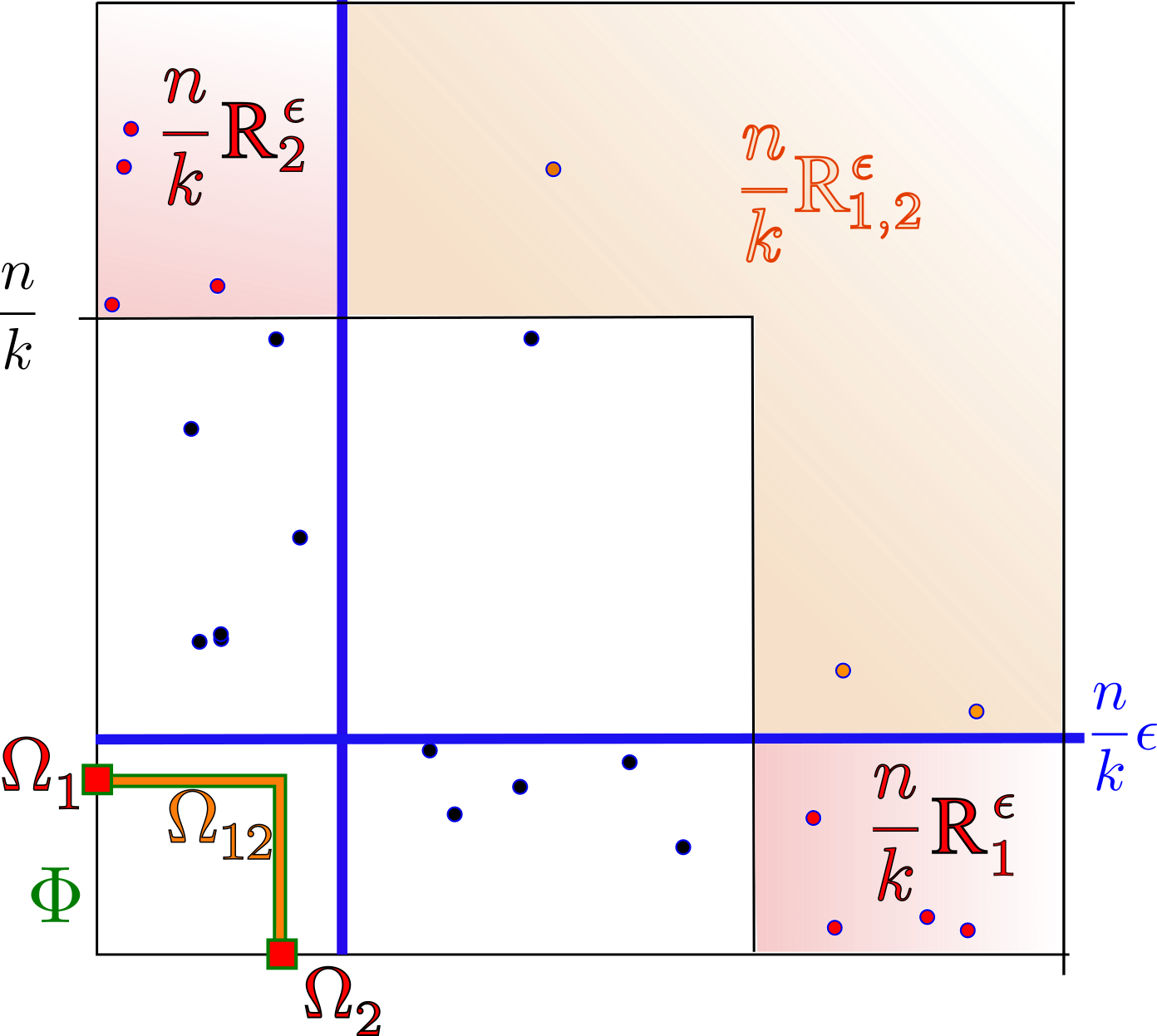
Figure 3: Estimation procedure

The coefficients $(\widehat{\mathcal{M}}(\alpha))_{\alpha\subset\{1,\ldots,d\}}$ related to the cones $\mathcal{C}_{\alpha}$ constitute a summary representation of the dependence structure. This representation is sparse as soon as the $\mu_{n}^{\alpha,\epsilon}$ are positive only for a few groups of features $\alpha$ (compared to the total number of groups or sub-cones, $2^{d}$ namely). It is is low-dimensional as soon as each of these groups $\alpha$ is of small cardinality, or equivalently the corresponding sub-cones are low-dimensional compared with $d$.

In fact, $\widehat{\mathcal{M}}(\alpha)$ is (up to a normalizing constant) an empirical version of the conditional probability that $T(\mathbf{X})$ belongs to the rectangle $rR_{\alpha}^{\epsilon}$, given that $\|T(\mathbf{X})\|$ exceeds a large threshold $r$. Indeed, as explained in Remark 1,

$$\mathcal{M}(\alpha)=\lim_{r\to\infty}\mu([\mathbf{0},\mathbf{1}]^{c})~{}~{}\mathbb{P}(T(\mathbf{X})\in rR_{\alpha}^{\epsilon}~{}|~{}\|T(\mathbf{X})\|\geq r).$$ (3.4)

The remaining of this section is devoted to obtaining non-asymptotic upper bounds on the error $||\widehat{\mathcal{M}}-\mathcal{M}||_{\infty}$. The main result is stated in Theorem 1. Before all, notice that the error may be obviously decomposed as the sum of a stochastic term and a bias term inherent to the $\epsilon$-thickening approach:

$$||\widehat{\mathcal{M}}-\mathcal{M}||_{\infty} ~{}=~{}\max_{\alpha}|\mu_{n}(R_{\alpha}^{\epsilon})-\mu(\mathcal{C}_{\alpha})|$$

$$~{}\leq~{}~{}\max_{\alpha}|\mu-\mu_{n}|(R_{\alpha}^{\epsilon})~{}+~{}\max_{\alpha}|\mu(R_{\alpha}^{\epsilon})-\mu(\mathcal{C}_{\alpha})|~{}.$$ (3.5)

Here and beyond, for notational convenience, we simply denotes ‘$\alpha$’ for ‘$\alpha$ non empty subset of $\{1,\;\ldots,\;d\}$’. The main steps of the argument leading to Theorem 1 are as follows. First, obtain a uniform upper bound on the error $|\mu_{n}-\mu|$ restricted to a well chosen VC class of rectangles (Subsection 3.3), and deduce an uniform bound on $|\mu_{n}-\mu|(R_{\alpha}^{\epsilon})$ (Subsection 3.4). Finally, using the regularity assumptions (Assumption 2 and Assumption 3), bound the difference $|\mu(R_{\alpha}^{\epsilon})-\mu(\mathcal{C}_{\alpha})|$ (Subsection 3.5).

3.3 Preliminaries: uniform approximation over a VC-class of rectangles

This subsection builds on the theory developed in Goix et al. (2015), where a non-asymptotic bound is stated on the estimation of the stable tail dependence function (STDF) defined in (2.10). The STDF $l$ is related to the class of sets of the form $[\mathbf{0},\mathbf{v}]^{c}$ (or $[\mathbf{u},\boldsymbol{\infty}]^{c}$ depending on which standardization is used), and an equivalent definition is

$$l(\mathbf{x}):=\lim_{t\to\infty}t\tilde{F}(t^{-1}\mathbf{x})=\mu([\mathbf{0},\mathbf{x}^{-1}]^{c})$$ (3.6)

with $\tilde{F}(\mathbf{x})=(1-F)\big{(}(1-F_{1})^{\leftarrow}(x_{1}),\ldots,(1-F_{d})^{\leftarrow}(x_{d})\big{)}$. Here the notation $(1-F_{j})^{\leftarrow}(x_{j})$ denotes the quantity $\sup\{y\,:\;1-F_{j}(y)\geq x_{j}\}$. Recall that the marginally uniform variable $\mathbf{U}$ is defined by $U^{j}=1-F_{j}(X^{j})$ ($1\leq j\leq d$). Then in terms of standardized variables $U^{j}$,

$$\tilde{F}(\mathbf{x})=\mathbb{P}\Big{(}\bigcup_{j=1}^{d}\{U^{j}<x_{j}\}\Big{)}=\mathbb{P}(\mathbf{U}\in[\mathbf{x},\boldsymbol{\infty}[^{c})=\mathbb{P}(\mathbf{V}\in[\mathbf{0},\mathbf{x}^{-1}]^{c}).$$ (3.7)

A natural estimator of $l$ is its empirical version defined as follows, see Huang (1992), Qi (1997), Drees and Huang (1998), Einmahl et al. (2006), Goix et al. (2015):

$$l_{n}(\mathbf{x}) =\frac{1}{k}~{}\sum_{i=1}^{n}\mathds{1}_{\{X_{i}^{1}\geq X^{1}_{(n-\lfloor kx_{1}\rfloor+1)}\text{~{}~{}or~{}~{}}\ldots\text{~{}~{}or~{}~{}}X_{i}^{d}\geq X^{d}_{(n-\lfloor kx_{d}\rfloor+1)}\}}~{}.$$ (3.8)

The expression is indeed suggested by the definition of $l$ in (3.6), with all distribution functions and univariate quantiles replaced by their empirical counterparts, and with $t$ replaced by $n/k$. The following lemma allows to derive alternative expressions for the empirical version of the STDF.

Lemma 3.

Consider the rank transformed variables $\mathbf{\widehat{U}}_{i}=(\mathbf{\widehat{V}}_{i})^{-1}=(1-\widehat{F}_{j}(X_{i}^{j}))_{1\leq j\leq d}$ for $i=1,\ldots,n$. Then, for $(i,j)\in\{1,\ldots,n\}\times\{1,\ldots,d\}$, with probability one,

$$\widehat{U}_{i}^{j}\leq\frac{k}{n}x_{j}^{-1}~{}\Leftrightarrow~{}\widehat{V}_{i}^{j}\geq\frac{n}{k}x_{j}~{}\Leftrightarrow~{}X_{i}^{j}\geq X_{(n-\lfloor kx_{j}^{-1}\rfloor+1)}^{j}~{}\Leftrightarrow~{}U_{i}^{j}\leq U_{(\lfloor kx_{j}^{-1}\rfloor)}^{j}~{}.$$

The proof of Lemma 3 is standard and is provided in A for completeness. By Lemma 3, the following alternative expression of $l_{n}(\mathbf{x})$ holds true:

$$l_{n}(\mathbf{x})=\frac{1}{k}~{}\sum_{i=1}^{n}\mathds{1}_{\{U_{i}^{1}~{}\leq~{}U^{1}_{([kx_{1}])}\text{~{}~{}or~{}~{}}\ldots\text{~{}~{}or~{}~{}}U_{i}^{d}~{}\leq~{}U^{d}_{([kx_{d}])}\}}=\mu_{n}\left([\mathbf{0},\mathbf{x}^{-1}]^{c}\right).$$ (3.9)

Thus, bounding the error $|\mu_{n}-\mu|([\mathbf{0},\mathbf{x}^{-1}]^{c})$ is the same as bounding $|l_{n}-l|(\mathbf{x})$.

Asymptotic properties of this empirical counterpart have been studied in Huang (1992), Drees and Huang (1998), Embrechts et al. (2000) and de Haan and Ferreira (2006) in the bivariate case, and Qi (1997), Einmahl et al. (2012). in the general multivariate case. In Goix et al. (2015), a non-asymptotic bound is established on the maximal deviation

$$\sup_{0\leq\mathbf{x}\leq T}|l(\mathbf{x})-l_{n}(\mathbf{x})|$$

for a fixed $T>0$, or equivalently on

$$\sup_{1/T\leq\mathbf{x}}\left|\mu([\mathbf{0},\mathbf{x}]^{c})-\mu_{n}([\mathbf{0},\mathbf{x}]^{c})\right|.$$

The exponent measure $\mu$ is indeed easier to deal with when restricted to the class of sets of the form $[\mathbf{0},\mathbf{x}]^{c}$, which is fairly simple in the sense that it has finite VC dimension.

In the present work, an important step is to bound the error on the class of $\epsilon$-thickened rectangles $R_{\alpha}^{\epsilon}$. This is achieved by using a more general class $R(\mathbf{x},\mathbf{z},\alpha,\beta)$, which includes (contrary to the collection of sets $[\mathbf{0},\mathbf{x}]^{c}$) the $R_{\alpha}^{\epsilon}$’s . This flexible class is defined by

$$R(\mathbf{x},\mathbf{z},\alpha,\beta) ~{}=~{}\Big{\{}\mathbf{y}\in[0,\infty]^{d},~{}~{}y_{j}\geq x_{j}~{}~{}\text{ for }j\in\alpha,$$

$$~{}~{}~{}~{}~{}~{}~{}~{}~{}~{}~{}~{}~{}~{}~{}~{}~{}~{}~{}~{}~{}~{}~{}~{}~{}~{}y_{j}<z_{j}~{}~{}\text{ for }j\in\beta\quad\Big{\}},~{}~{}~{}\mathbf{x},\mathbf{z}\in[0,\infty]^{d}.$$ (3.10)

Thus,

$$\mu_{n}\left(R(\mathbf{x},\mathbf{z},\alpha,\beta)\right) ~{}=~{}\frac{1}{k}\sum_{i=1}^{n}\mathds{1}_{\{\widehat{V}_{i}^{j}~{}\geq~{}\frac{n}{k}x_{j}\text{ for }j\in\alpha\text{ ~{}and~{} }\widehat{V}_{i}^{j}~{}<~{}\frac{n}{k}x_{j}\text{ for }j\in\beta\}}~{}.$$

Then, define the functional $g_{\alpha,\beta}$ (which plays the same role as the STDF) as follows: for $\mathbf{x}\in[0,\infty]^{d}\setminus\{\boldsymbol{\infty}\}$, $\mathbf{z}\in[0,\infty]^{d}$, $\alpha\subset\{1,\ldots,d\}\setminus\emptyset$ and $\beta\subset\{1,\ldots,d\}$, let

$$g_{\alpha,\beta}(\mathbf{x},\mathbf{z})~{}~{}=~{}~{}\lim_{t\to\infty}t\tilde{F}_{\alpha,\beta}(t^{-1}\mathbf{x},t^{-1}\mathbf{z}),\text{~{}~{}with}$$ (3.11)

$$\tilde{F}_{\alpha,\beta}(\mathbf{x},\mathbf{z})~{}~{}=~{}~{}\mathbb{P}\left[\left\{U^{j}\leq x_{j}~{}~{}\text{ for }j\in\alpha\right\}~{}~{}\bigcap~{}~{}\left\{U^{j}>z_{j}~{}~{}\text{ for }j\in\beta\right\}\right].$$ (3.12)

Notice that $\tilde{F}_{\alpha,\beta}(\mathbf{x},\mathbf{z})$ is an extension of the non-asymptotic approximation $\tilde{F}$ in (3.6). By (3.11) and (3.12), we have

$$g_{\alpha,\beta}(\mathbf{x},\mathbf{z}) =\lim_{t\to\infty}t\mathbb{P}\left[\left\{U^{j}\leq t^{-1}x_{j}~{}\text{ for }j\in\alpha\right\}~{}\bigcap~{}\left\{U^{j}>t^{-1}z_{j}~{}\text{ for }j\in\beta\right\}\right]$$

$$=\lim_{t\to\infty}t\mathbb{P}\left[\mathbf{V}\in tR(\mathbf{x}^{-1},\mathbf{z}^{-1},\alpha,~{}\beta)\right]~{},$$

so that using (2.4),

$$g_{\alpha,\beta}(\mathbf{x},\mathbf{z})=\mu([R(\mathbf{x}^{-1},\mathbf{z}^{-1},\alpha,~{}\beta)]).$$ (3.13)

The following lemma makes the relation between $g_{\alpha,\beta}$ and the angular measure $\Phi$ explicit. Its proof is given in A.

Lemma 4.

The function $g_{\alpha,\beta}$ can be represented as follows:

$$g_{\alpha,\beta}(\mathbf{x},\mathbf{z})=\int_{S^{d-1}}\left(\bigwedge_{j\in\alpha}{w_{j}x_{j}}-\bigvee_{j\in\beta}w_{j}z_{j}\right)_{+}~{}\Phi(\mathrm{d}\mathbf{w})~{},$$

where $u\wedge v=\min\{u,v\}$, $u\vee v=\max\{u,v\}$ and $u_{+}=\max\{u,0\}$ for any $(u,v)\in\mathbb{R}^{2}$. Thus, $g_{\alpha,\beta}$ is homogeneous and satisfies

$$|g_{\alpha,\beta}(\mathbf{x},\mathbf{z})-g_{\alpha,\beta}(\mathbf{x}^{\prime},\mathbf{z}^{\prime})|~{}~{}\leq~{}~{}\sum_{j\in\alpha}|x_{j}-x_{j}^{\prime}|~{}+~{}\sum_{j\in\beta}|z_{j}-z_{j}^{\prime}|~{},$$

Remark 3.

Lemma 4 shows that the functional $g_{\alpha,\beta}$, which plays the same role as a the STDF, enjoys a Lipschitz property.

We now define the empirical counterpart of $g_{\alpha,\beta}$ (mimicking that of the empirical STDF $l_{n}$ in (3.8) ) by

$$g_{n,\alpha,\beta}(\mathbf{x},\mathbf{z})=\frac{1}{k}~{}\sum_{i=1}^{n}\mathds{1}_{\{X_{i}^{j}\geq X^{j}_{(n-\lfloor kx_{j}\rfloor+1)}~{}~{}\text{for}~{}j\in\alpha\text{~{}~{}~{}and~{}~{}~{}}X_{i}^{j}<X^{j}_{(n-\lfloor kx_{j}\rfloor+1)}~{}~{}\text{for}~{}j\in\beta\}}~{}.$$ (3.14)

As it is the case for the empirical STDF (see (3.9)), $g_{n,\alpha,\beta}$ has an alternative expression

$$g_{n,\alpha,\beta}(\mathbf{x},\mathbf{z}) =\frac{1}{k}~{}\sum_{i=1}^{n}\mathds{1}_{\{U_{i}^{j}~{}\leq~{}U^{j}_{([kx_{j}])}~{}~{}\text{for}~{}j\in\alpha\text{~{}~{}~{}and~{}~{}~{}}U_{i}^{j}~{}>~{}U^{j}_{([kx_{j}])}~{}~{}\text{for}~{}j\in\beta\}}$$

$$=\mu_{n}\left(R(\mathbf{x}^{-1},\mathbf{z}^{-1},\alpha,~{}\beta)\right),$$ (3.15)

where the last equality comes from the equivalence $\widehat{V}_{i}^{j}\geq\frac{n}{k}x_{j}\Leftrightarrow U_{i}^{j}\leq U_{(\lfloor kx_{j}^{-1}\rfloor)}^{j}$ (Lemma 3) and from the expression $\mu_{n}(\,\cdot\,)=\frac{1}{k}\sum_{i=1}^{n}\mathds{1}_{\mathbf{\widehat{V}}_{i}\in\frac{n}{k}(\,\cdot\,)}$, definition (3.2).

The proposition below extends the result of Goix et al. (2015), by deriving an analogue upper bound on the maximal deviation

$$\max_{\alpha,\beta}\sup_{0\leq\mathbf{x},\mathbf{z}\leq T}|g_{\alpha,\beta}(\mathbf{x},\mathbf{z})-g_{n,\alpha,\beta}(\mathbf{x},\mathbf{z})|~{},$$

or equivalently on

$$\max_{\alpha,\beta}~{}\sup_{1/T\leq\mathbf{x},\mathbf{z}}\left|\mu(R(\mathbf{x},\mathbf{z},\alpha,\beta))-\mu_{n}(R(\mathbf{x},\mathbf{z},\alpha,\beta))\right|~{}.$$

Here and beyond we simply denote ‘$\alpha,\beta$’ for ‘$\alpha$ non-empty subset of $\{1,\ldots,d\}\setminus\emptyset$ and $\beta$ subset of $\{1,\ldots,d\}$’. We also recall that comparison operators between two vectors (or between a vector and a real number) are understood component-wise, i.e.  ‘$\mathbf{x}\leq\mathbf{z}$’ means ‘$x_{j}\leq z_{j}$ for all $1\leq j\leq d$’ and for any real number $T$, ‘$\mathbf{x}\leq T$’ means ‘$x_{j}\leq T$ for all $1\leq j\leq d$’.

Proposition 1.

Let $T\geq\frac{7}{2}(\frac{\log d}{k}+1)$, and $\delta\geq e^{-k}$. Then there is a universal constant $C$, such that for each $n>0$, with probability at least $1-\delta$,

$$\max_{\alpha,\beta}\sup_{0\leq\mathbf{x},\mathbf{z}\leq T} \left|g_{n,\alpha,\beta}(\mathbf{x},\mathbf{z})-g_{\alpha,\beta}(\mathbf{x},\mathbf{z})\right|~{}\leq~{}Cd\sqrt{\frac{2T}{k}\log\frac{d+3}{\delta}}$$ (3.16)

$$~{}~{}~{}~{}~{}~{}~{}~{}~{}~{}~{}~{}~{}~{}~{}~{}~{}~{}~{}~{}~{}~{}~{}+\max_{\alpha,\beta}\sup_{0\leq\mathbf{x},\mathbf{z}\leq 2T}\left|\frac{n}{k}\tilde{F}_{\alpha,\beta}(\frac{k}{n}\mathbf{x},\frac{k}{n}\mathbf{z})-g_{\alpha,\beta}(\mathbf{x},\mathbf{z})\right|.$$

The second term on the right hand side of the inequality is an asymptotic bias term which goes to $0$ as $n\to\infty$ (see Remark 12).

The proof follows the same lines as that of Theorem 6 in Goix et al. (2015) and is detailed in A. Here is the main argument.

The empirical estimator is based on the empirical measure of ‘extreme’ regions, which are hit only with low probability. It is thus enough to bound maximal deviations on such low probability regions. The key consists in choosing an adaptive VC class which only covers the latter regions (after standardization to uniform margins), namely a VC class composed of sets of the kind $\frac{k}{n}R(\mathbf{x}^{-1},\mathbf{z}^{-1},\alpha,\beta)^{-1}$. In Goix et al. (2015), VC-type inequalities have been established that incorporate $p$, the probability of hitting the class at all. Applying these inequalities to the particular class of rectangles gives the result.

3.4 Bounding $|\mu_{n}-\mu|(R_{\alpha}^{\epsilon})$ uniformly over $\alpha$

The aim of this subsection is to exploit the previously established bound on the deviations on rectangles, to obtain another uniform bound for $|\mu_{n}-\mu|(R_{\alpha}^{\epsilon})$, for $\epsilon>0$ and $\alpha\subset\{1,\ldots,d\}$. In the remainder of the paper, $\bar{\alpha}$ denotes the complementary set of $\alpha$ in $\{1,\ldots,d\}$. Notice that directly from their definitions (2.13) and (3.10), $R_{\alpha}^{\epsilon}$ and $R(\mathbf{x},\mathbf{z},\alpha,\beta)$ are linked by:

$$R_{\alpha}^{\epsilon}=R(\boldsymbol{\epsilon},\boldsymbol{\epsilon},\alpha,\bar{\alpha})\cap[\mathbf{0},\mathbf{1}]^{c}=R(\boldsymbol{\epsilon},\boldsymbol{\epsilon},\alpha,\bar{\alpha})\setminus R(\boldsymbol{\epsilon},\boldsymbol{\tilde{\epsilon}},\alpha,\{1,\ldots,d\})$$

where $\boldsymbol{\tilde{\epsilon}}$ is defined by $\boldsymbol{\tilde{\epsilon}}_{j}=\mathds{1}_{j\in\alpha}+\epsilon\mathds{1}_{j\notin\alpha}$ for all $j\in\{1,\ldots,d\}$. Indeed, we have: $R(\boldsymbol{\epsilon},\boldsymbol{\epsilon},\alpha,\bar{\alpha})\cap[\mathbf{0},\mathbf{1}]=R(\boldsymbol{\epsilon},\boldsymbol{\tilde{\epsilon}},\alpha,\{1,\ldots,d\})$. As a result, for $\epsilon<1$,

$$\sup_{\epsilon\leq\mathbf{x},\mathbf{z}}|\mu_{n}-\mu|\left(R_{\alpha}^{\epsilon}\right)\leq 2\sup_{\epsilon\leq\mathbf{x},\mathbf{z}}|\mu_{n}-\mu|\left(R(\mathbf{x},~{}\mathbf{z},~{}\alpha,~{}\bar{\alpha})\right).$$

On the other hand, from (3.3) and (3.13) we have

$$\sup_{\epsilon\leq\mathbf{x},\mathbf{z}}|\mu_{n}-\mu|\left(R(\mathbf{x},~{}\mathbf{z},~{}\alpha,~{}\bar{\alpha})\right)~{}=~{}\sup_{0\leq\mathbf{x},\mathbf{z}\leq\epsilon^{-1}}\left|g_{n,\alpha,\bar{\alpha}}(\mathbf{x},\mathbf{z})-g_{\alpha,\bar{\alpha}}(\mathbf{x},\mathbf{z})\right|.$$

Then Proposition 1 applies with $T=1/\epsilon$ and the following result holds true.

Corollary 1.

Let $0<\epsilon\leq(\frac{7}{2}(\frac{\log d}{k}+1))^{-1}$, and $\delta\geq e^{-k}$. Then there is a universal constant $C$, such that for each $n>0$, with probability at least $1-\delta$,

$$\max_{\alpha}\sup_{\epsilon\leq\mathbf{x},\mathbf{z}} \left|(\mu_{n}-\mu)(R_{\alpha}^{\epsilon})\right|~{}\leq~{}Cd\sqrt{\frac{1}{\epsilon k}\log\frac{d+3}{\delta}}$$ (3.17)

$$~{}~{}~{}~{}~{}~{}~{}~{}~{}~{}~{}~{}~{}~{}~{}~{}~{}~{}~{}~{}~{}~{}~{}+\max_{\alpha,\beta}\sup_{0\leq\mathbf{x},\mathbf{z}\leq 2\epsilon^{-1}}\left|\frac{n}{k}\tilde{F}_{\alpha,\beta}(\frac{k}{n}\mathbf{x},\frac{k}{n}\mathbf{z})-g_{\alpha,\beta}(\mathbf{x},\mathbf{z})\right|.$$

3.5 Bounding $|\mu(R_{\alpha}^{\epsilon})-\mu(\mathcal{C}_{\alpha})|$ uniformly over $\alpha$

In this section, an upper bound on the bias induced by handling $\epsilon$-thickened rectangles is derived. As the rectangles $R_{\alpha}^{\epsilon}$ defined in (2.13) do not correspond to any set of angles on the sphere $S_{\infty}^{d-1}$, we also define the $(\epsilon,\epsilon^{\prime})$-thickened cones

$$\mathcal{C}_{\alpha}^{\epsilon,\epsilon^{\prime}}~{}=\{\mathbf{v}\geq 0,~{}\|\mathbf{v}\|_{\infty}\geq 1,~{}v_{j}>\epsilon\|\mathbf{v}\|_{\infty}~{}\text{ for }j\in\alpha,~{}v_{j}\leq\epsilon^{\prime}\|\mathbf{v}\|_{\infty}~{}\text{ for }j\notin\alpha\},$$ (3.18)

which verify $\mathcal{C}_{\alpha}^{\epsilon,0}\subset R_{\alpha}^{\epsilon}\subset\mathcal{C}_{\alpha}^{0,\epsilon}.$ Define the corresponding $(\epsilon,\epsilon^{\prime})$-thickened sub-sphere

$$\Omega_{\alpha}^{\epsilon,\epsilon^{\prime}}=~{}~{}\big{\{}\mathbf{x}\in S^{d-1}_{\infty},~{}~{}x_{i}>\epsilon~{}~{}\text{ for }i\in\alpha~{},~{}~{}x_{i}\leq\epsilon^{\prime}~{}~{}\text{ for }i\notin\alpha\big{\}}=~{}~{}\mathcal{C}_{\alpha}^{\epsilon,\epsilon^{\prime}}\cap S^{d-1}_{\infty}.$$ (3.19)

It is then possible to approximate rectangles $R_{\alpha}^{\epsilon}$ by the cones $\mathcal{C}_{\alpha}^{\epsilon,0}$ and $\mathcal{C}_{\alpha}^{0,\epsilon}$, and then $\mu(R_{\alpha}^{\epsilon})$ by $\Phi(\Omega_{\alpha}^{\epsilon,\epsilon^{\prime}})$ in the sense that

$$\Phi(\Omega_{\alpha}^{\epsilon,0})=\mu(\mathcal{C}_{\alpha}^{\epsilon,0})\leq\mu(R_{\alpha}^{\epsilon})\leq\mu(\mathcal{C}_{\alpha}^{0,\epsilon})=\Phi(\Omega_{\alpha}^{0,\epsilon}).$$ (3.20)

The next result (proved in A) is a preliminary step toward a bound on $|\mu(R_{\alpha}^{\epsilon})-\mu(\mathcal{C}_{\alpha})|$. It is easier to use the absolute continuity of $\Phi$ instead of that of $\mu$, since the rectangles $R_{\alpha}^{\epsilon}$ are not bounded contrary to the sub-spheres $\Omega_{\alpha}^{\epsilon,\epsilon^{\prime}}$.

Lemma 5.

For every $\emptyset\neq\alpha\subset\{1,\ldots,d\}$ and $0<\epsilon,\epsilon^{\prime}<1/2$, we have

$$|\Phi(\Omega_{\alpha}^{\epsilon,\epsilon^{\prime}})-\Phi(\Omega_{\alpha})|~{}\leq~{}M|\alpha|^{2}\epsilon~{}+~{}Md\epsilon^{\prime}~{}.$$

Now, notice that

$$\Phi(\Omega_{\alpha}^{\epsilon,0})-\Phi(\Omega_{\alpha})\leq\mu(R_{\alpha}^{\epsilon})-\mu(\mathcal{C}_{\alpha})\leq\Phi(\Omega_{\alpha}^{0,\epsilon})-\Phi(\Omega_{\alpha}).$$

We obtain the following proposition.

Proposition 2.

For every non empty set of indices $\emptyset\neq\alpha\subset\{1,\ldots,d\}$ and $\epsilon>0$,

$$|\mu(R_{\alpha}^{\epsilon})-\mu(\mathcal{C}_{\alpha})|\leq Md^{2}\epsilon$$

3.6 Main result

We can now state the main result of the paper, revealing the accuracy of the estimate (3.3).

Theorem 1.

There is an universal constant $C>0$ such that for every $n,~{}k,~{}\epsilon,~{}\delta$ verifying $\delta\geq e^{-k}$, $0<\epsilon<1/2$ and $\epsilon\leq(\frac{7}{2}(\frac{\log d}{k}+1))^{-1}$, the following inequality holds true with probability greater than $1-\delta$:

$$\|\widehat{\mathcal{M}}-\cal{M}\|_{\infty} ~{}\leq~{}Cd\left(\sqrt{\frac{1}{\epsilon k}\log\frac{d}{\delta}}+Md\epsilon\right)$$

$$~{}~{}~{}~{}~{}~{}~{}~{}~{}~{}~{}+~{}4\max_{\begin{subarray}{c}\alpha~{}\subset~{}\{1,\ldots,d\}\\ \alpha\neq\emptyset\end{subarray}}~{}~{}\sup_{0\leq\mathbf{x},\mathbf{z}\leq\frac{2}{\epsilon}}\left|\frac{n}{k}\tilde{F}_{\alpha,\bar{\alpha}}(\frac{k}{n}\mathbf{x},\frac{k}{n}\mathbf{z})-g_{\alpha,\bar{\alpha}}(\mathbf{x},\mathbf{z})\right|.$$

Note that $\frac{7}{2}(\frac{\log d}{k}+1)$ is smaller than $4$ as soon as $\log d/k<1/7$, so that a sufficient condition on $\epsilon$ is $\epsilon<1/4$. The last term in the right hand side is a bias term which goes to zero as $n\to\infty$ (see Remark 12). The term $Md\epsilon$ is also a bias term, which represents the bias induced by considering $\epsilon$-thickened rectangles. It depends linearly on the sparsity constant $M$ defined in Assumption 3. The value $k$ can be interpreted as the effective number of observations used in the empirical estimate, i.e. the effective sample size for tail estimation. Considering classical inequalities in empirical process theory such as VC-bounds, it is thus no surprise to obtain one in $O(1/\sqrt{k})$. Too large values of $k$ tend to yield a large bias, whereas too small values of $k$ yield a large variance. For a more detailed discussion on the choice of $k$ we recommend Einmahl et al. (2009).

The proof is based on decomposition (3.5). The first term $\sup_{\alpha}|\mu_{n}(R_{\alpha}^{\epsilon})-\mu(R_{\alpha}^{\epsilon})|$ on the right hand side of (3.5) is bounded using Corollary 1, while Proposition 2 allows to bound the second one (bias term stemming from the tolerance parameter $\epsilon$). Introduce the notation

$$\text{bias}(\alpha,n,k,\epsilon) =4\sup_{0\leq\mathbf{x},\mathbf{z}\leq\frac{2}{\epsilon}}\left|\frac{n}{k}\tilde{F}_{\alpha,\bar{\alpha}}(\frac{k}{n}\mathbf{x},\frac{k}{n}\mathbf{z})-g_{\alpha,\bar{\alpha}}(\mathbf{x},\mathbf{z})\right|.$$ (3.21)

With probability at least $1-\delta$,

$$\forall~{}\emptyset\neq\alpha\subset\{1,\ldots,d\},~{}~{}~{}~{}~{}~{}~{}~{}$$

$$\left|\mu_{n}(R_{\alpha}^{\epsilon})-\mu(\mathcal{C}_{\alpha})\right|~{}\leq~{} Cd\sqrt{\frac{1}{\epsilon k}\log\frac{d+3}{\delta}}~{}+~{}~{}\text{bias}(\alpha,n,k,\epsilon)+Md^{2}\epsilon~{}.$$

The upper bound stated in Theorem 1 follows.

Remark 4.

(Thresholding the estimator) In practice, we have to deal with non-asymptotic noisy data, so that many $\widehat{\mathcal{M}}(\alpha)$’s have very small values though the corresponding $\mathcal{M}(\alpha)$’s are null. One solution is thus to define a threshold value, for instance a proportion $p$ of the averaged mass over all the faces $\alpha$ with positive mass, i.e. $\text{threshold}=p|A|^{-1}\sum_{\alpha}\widehat{\mathcal{M}}(\alpha)$ with $A=\{\alpha,~{}\widehat{\mathcal{M}}(\alpha)>0\}$ . Let us define $\widetilde{\mathcal{M}}(\alpha)$ the obtained thresholded $\widehat{\mathcal{M}}(\alpha)$. Then the estimation error satisfies:

$$\|\widetilde{\mathcal{M}}-\mathcal{M}\|_{\infty} \leq\|\widetilde{\mathcal{M}}-\widehat{\mathcal{M}}\|_{\infty}+\|\widehat{\mathcal{M}}-\mathcal{M}\|_{\infty}$$

$$\leq p|A|^{-1}\sum_{\alpha}\widehat{\mathcal{M}}(\alpha)+\|\widehat{\mathcal{M}}-\mathcal{M}\|_{\infty}$$

$$\leq p|A|^{-1}\sum_{\alpha}\mathcal{M}(\alpha)+p|A|^{-1}\sum_{\alpha}|\widehat{\mathcal{M}}(\alpha)-\mathcal{M}(\alpha)|$$

$$~{}~{}~{}~{}~{}~{}~{}~{}~{}~{}~{}~{}~{}~{}~{}~{}~{}~{}~{}~{}~{}~{}~{}~{}~{}~{}~{}~{}~{}~{}~{}~{}~{}~{}~{}~{}~{}~{}~{}~{}~{}~{}~{}~{}~{}~{}~{}~{}~{}~{}~{}~{}~{}~{}~{}~{}~{}~{}~{}+\|\widehat{\mathcal{M}}-\mathcal{M}\|_{\infty}$$

$$\leq(p+1)\|\widehat{\mathcal{M}}-\mathcal{M}\|_{\infty}+p|A|^{-1}\mu([0,1]^{c}).$$

It is outside the scope of this paper to study optimal values for $p$. However, Remark 5 writes the estimation procedure as an optimization problem, thus exhibiting a link between thresholding and $L^{1}$-regularization.

Remark 5.

(Underlying risk minimization problems) Our estimate $\widehat{\mathcal{M}}(\alpha)$ can be interpreted as a solution of an empirical risk minimization problem inducing a conditional empirical risk $\widehat{R}_{n}$. When adding a $L^{1}$ regularization term to this problem, we recover $\widetilde{\mathcal{M}}(\alpha)$, the thresholded estimate.

First recall that $\widehat{\mathcal{M}}(\alpha)$ is defined for $\alpha\subset\{1,\ldots,d\},~{}\alpha\neq\emptyset$ by $\widehat{\mathcal{M}}(\alpha)=1/k\sum_{i=1}^{n}\mathds{1}_{\frac{k}{n}\hat{\mathbf{V}}_{i}\in R_{\alpha}^{\epsilon}}$. As $R_{\alpha}^{\epsilon}\subset[\mathbf{0},\mathbf{1}]^{c}$, we may write

$$\widehat{\mathcal{M}}(\alpha)=\Big{(}\frac{n}{k}\mathcal{P}_{n}(\frac{k}{n}\|\hat{\mathbf{V}}_{1}\|\geq 1)\Big{)}~{}~{}\Big{(}\frac{1}{n}\sum_{i=1}^{n}\frac{\mathds{1}_{\frac{k}{n}\hat{\mathbf{V}}_{i}\in R_{\alpha}^{\epsilon}}\mathds{1}_{\frac{k}{n}\|\hat{\mathbf{V}}_{i}\|\geq 1}}{\mathcal{P}_{n}(\frac{k}{n}\|\hat{\mathbf{V}}_{1}\|\geq 1)}\Big{)},$$

where the last term is the empirical expectation of $Z_{n,i}(\alpha)=\mathds{1}_{\frac{k}{n}\hat{\mathbf{V}}_{i}\in R_{\alpha}^{\epsilon}}$ conditionnaly to the event $\{\|\frac{k}{n}\hat{\mathbf{V}}_{1}\|\geq 1\}$, and $\mathcal{P}_{n}(\frac{k}{n}\|\hat{\mathbf{V}}_{1}\|\geq 1)=\frac{1}{n}\sum_{i=1}^{n}\mathds{1}_{\frac{k}{n}\|\hat{\mathbf{V}}_{i}\|\geq 1}$. According to Lemma 3, for each fixed margin $j$, $\hat{V}_{i}^{j}\geq\frac{n}{k}$ if, and only if $X_{i}^{j}\geq X_{(n-k+1)}^{j}$, which happens for $k$ observations exactly. Thus,

$$\mathcal{P}_{n}(\frac{k}{n}\|\hat{\mathbf{V}}_{1}\|\geq 1)=\frac{1}{n}\sum_{i=1}^{n}\mathds{1}_{\exists j,\hat{\mathbf{V}}_{i}^{j}\geq\frac{n}{k}}\in\left[\frac{k}{n},\frac{dk}{n}\right].$$

If we define $\tilde{k}=\tilde{k}(n)\in[k,dk]$ such that $\mathcal{P}_{n}(\frac{k}{n}\|\hat{\mathbf{V}}_{1}\|\geq 1)=\frac{\tilde{k}}{n}$, we then have

$$\widehat{\mathcal{M}}(\alpha) =\frac{\tilde{k}}{k}~{}~{}\left(\frac{1}{n}\sum_{i=1}^{n}\frac{\mathds{1}_{\frac{k}{n}\hat{\mathbf{V}}_{i}\in R_{\alpha}^{\epsilon}}\mathds{1}_{\frac{k}{n}\|\hat{\mathbf{V}}_{i}\|\geq 1}}{\mathcal{P}_{n}(\frac{k}{n}\|\hat{\mathbf{V}}_{1}\|\geq 1)}\right)$$

$$=\frac{\tilde{k}}{k}~{}~{}\operatorname{argmin}_{m_{\alpha}>0}\sum_{i=1}^{n}(Z_{n,i}(\alpha)-m_{\alpha})^{2}\mathds{1}_{\frac{k}{n}\|\hat{\mathbf{V}}_{i}\|\geq 1},$$

Considering now the $(2^{d}-1)$-vector $\widehat{\mathcal{M}}$ and $\|.\|_{2,\alpha}$ the $L^{2}$-norm on $\mathbb{R}^{2^{d}-1}$, we immediatly have (since $k(n)$ does not depend on $\alpha$)

$$\widehat{\mathcal{M}}=\frac{\tilde{k}}{k}\operatorname{argmin}_{m\in\mathbb{R}^{2^{d}-1}}\widehat{R_{n}}(m),$$ (3.22)

where $\widehat{R_{n}}(m)=\sum_{i=1}^{n}\|Z_{n,i}-m\|_{2,\alpha}^{2}\mathds{1}_{\frac{k}{n}\|\hat{\mathbf{V}}_{i}\|\geq 1}$ is the $L^{2}$-empirical risk of $m$, restricted to extreme observations, namely to observations $\mathbf{X}_{i}$ satisfying $\|\hat{\mathbf{V}}_{i}\|\geq\frac{n}{k}$. Then, up to a constant $\frac{\tilde{k}}{k}=\Theta(1)$, $\widehat{\mathcal{M}}$ is solution of an empirical conditional risk minimization problem. Define the non-asymptotic theoretical risk $R_{n}(m)$ for $m\in\mathbb{R}^{2^{d}-1}$ by

$$R_{n}(m)=\mathbb{E}\left[\|Z_{n}-m\|_{2,\alpha}^{2}\Big{|}\|\frac{k}{n}\mathbf{V}_{1}\|_{\infty}\geq 1\right]$$

with $Z_{n}:=Z_{n,1}$. Then one can show (see A) that $Z_{n}$, conditionally to the event $\{\|\frac{k}{n}\mathbf{V}_{1}\|\geq 1\}$, converges in distribution to a variable $Z_{\infty}$ which is a multinomial distribution on $\mathbb{R}^{2^{d}-1}$ with parameters $(n=1,p_{\alpha}=\frac{\mu(R_{\alpha}^{\epsilon})}{\mu([\mathbf{0},\mathbf{1}]^{c})},\alpha\in\{1,\ldots,n\},\alpha\neq\emptyset)$. In other words,

$$\mathbb{P}(Z_{\infty}(\alpha)=1)=\frac{\mu(R_{\alpha}^{\epsilon})}{\mu([\mathbf{0},\mathbf{1}]^{c})}$$

for all $\alpha\in\{1,\ldots,n\},\alpha\neq\emptyset$, and $\sum_{\alpha}Z_{\infty}(\alpha)=1$. Thus $R_{n}(m)\to R_{\infty}(m):=\mathbb{E}[\|Z_{\infty}-m\|_{2,\alpha}^{2}]$, which is the asymptotic risk. Moreover, the optimization problem

$$\min_{m\in\mathbb{R}^{2^{d}-1}}R_{\infty}(m)$$

admits $m=(\frac{\mu(R_{\alpha}^{\epsilon})}{\mu([\mathbf{0},\mathbf{1}]^{c})},\alpha\subset\{1,\ldots,n\},\alpha\neq\emptyset)$ as solution.

Considering the solution of the minimization problem (3.22), which happens to coincide with the definition of $\widehat{\mathcal{M}}$, makes then sense if the goal is to estimate $\mathcal{M}:=(\mu(R_{\alpha}^{\epsilon}),\alpha\in\{1,\ldots,n\},\alpha\neq\emptyset)$. As well as considering thresholded estimators $\widetilde{\mathcal{M}}(\alpha)$, since it amounts (up to a bias term) to add a $L^{1}$-penalization term to the underlying optimization problem: Let us consider

$$\min_{m\in\mathbb{R}^{2^{d}-1}}\widehat{R_{n}}(m)~{}+~{}\lambda\|m\|_{1,\alpha}$$

with $\|m\|_{1,\alpha}=\sum_{\alpha}|m(\alpha)|$ the $L^{1}$ norm on $\mathbb{R}^{2^{d}-1}$. In this optimization problem, only extreme observations are involved. It is a well known fact that solving it is equivalent to soft-thresholding the solution of the same problem without the penality term – and then, up to a bias term due to the soft-thresholding, it boils down to setting to zero features $m(\alpha)$ which are less than some fixed threshold $T(\lambda)$. This is an other interpretation on thresholding as defined in Remark 4.

4 Application to Anomaly Detection

4.1 Background on AD

What is Anomaly Detection ? From a machine learning perspective, AD can be considered as a specific classification task, where the usual assumption in supervised learning stipulating that the dataset contains structural information regarding all classes breaks down, see Roberts (1999). This typically happens in the case of two highly unbalanced classes: the normal class is expected to regroup a large majority of the dataset, so that the very small number of points representing the abnormal class does not allow to learn information about this class. Supervised AD consists in training the algorithm on a labeled (normal/abnormal) dataset including both normal and abnormal observations. In the semi-supervised context, only normal data are available for training. This is the case in applications where normal operations are known but intrusion/attacks/viruses are unknown and should be detected. In the unsupervised setup, no assumption is made on the data which consist in unlabeled normal and abnormal instances. In general, a method from the semi-supervised framework may apply to the unsupervised one, as soon as the number of anomalies is sufficiently weak to prevent the algorithm from fitting them when learning the normal behavior. Such a method should be robust to outlying observations.

Extremes and Anomaly Detection. As a matter of fact, ‘extreme’ observations are often more susceptible to be anomalies than others. In other words, extremal observations are often at the border between normal and abnormal regions and play a very special role in this context. As the number of observations considered as extreme (e.g. in a Peak-over-threshold analysis) typically constitute less than one percent of the data, a classical AD algorithm would tend to systematically classify all of them as abnormal: it is not worth the risk (in terms of ROC or precision-recall curve for instance) trying to be more accurate in low probability regions without adapted tools. Also, new observations outside the ‘observed support’ are most often predicted as abnormal. However, false positives (i.e. false alarms) are very expensive in many applications (e.g. aircraft predictive maintenance). It is thus of primal interest to develop tools increasing precision (i.e. the probability of observing an anomaly among alarms) on such extremal regions.

Contributions. The algorithm proposed in this paper provides a scoring function which ranks extreme observations according to their supposed degree of abnormality. This method is complementary to other AD algorithms, insofar as two algorithms (that described here, together with any other appropriate AD algorithm) may be trained on the same dataset. Afterwards, the input space may be divided into two regions – an extreme region and a non-extreme one– so that a new observation in the central region (resp. in the extremal region) would be classified as abnormal or not according to the scoring function issued by the generic algorithm (resp. the one presented here). The scope of our algorithm concerns both semi-supervised and unsupervised problems. Undoubtedly, as it consists in learning a ‘normal’ (i.e. not abnormal) behavior in extremal regions, it is optimally efficient when trained on ‘normal’ observations only. However it also applies to unsupervised situations. Indeed, it involves a non-parametric but relatively coarse estimation scheme which prevents from over-fitting normal data or fitting anomalies. As a consequence, this method is robust to outliers and also applies when the training dataset contains a (small) proportion of anomalies.

4.2 Algorithm: Detecting Anomalies among Multivariate EXtremes (DAMEX)

The purpose of this subsection is to explain the heuristic behind the use of multivariate EVT for Anomaly Detection, which is in fact a natural way to proceed when trying to describe the dependence structure of extreme regions. The algorithm is thus introduced in an intuitive setup, which matches the theoretical framework and results obtained in sections 2 and 3. The notations are the same as above: $\mathbf{X}=(X^{1},\ldots,X^{d})$ is a random vector in $\mathbb{R}^{d}$, with joint (resp. marginal) distribution $\mathbf{F}$ (resp. $F_{j}$, $j=1,\ldots,d$) and $\mathbf{X}_{1},.\ldots,\mathbf{X}_{n}\sim\mathbf{F}$ is an $\mathit{i.i.d.}$ sample. The first natural step to study the dependence between the margins $X^{j}$ is to standardize them, and the choice of standard Pareto margins (with c.d.f. $x\mapsto 1/x$) is convenient: Consider thus the $\mathbf{V}_{i}$’s and $\mathbf{\widehat{V}}_{i}$’s as defined in Section 2. One possible strategy to investigate the dependence structure of extreme events is to characterize, for each subset of features $\alpha\subset\{1,...,d\}$, the ‘correlation’ of these features given that one of them at least is large and the others are small. Formally, we associate to each such $\alpha$ a coefficient $\mathcal{M}(\alpha)$ reflecting the degree of dependence between the features $\alpha$. This coefficient is to be proportional to the expected number of points $\mathbf{V}_{i}$ above a large radial threshold ($\|\mathbf{V}\|_{\infty}>r$), verifying $V_{i}^{j}$ ‘large’ for $j\in\alpha$, while $V_{i}^{j}$ ‘small’ for $j\notin\alpha$. In order to define the notion of ‘large’ and ‘small’, fix a (small) tolerance parameter $0<\epsilon<1$. Thus, our focus is on the expected proportion of points ‘above a large radial threshold’ $r$ which belong to the truncated rectangles $R_{\alpha}^{\epsilon}$ defined in (2.13). More precisely, our goal is to estimate the above expected proportion, when the tolerance parameter $\epsilon$ goes to $0$.

The standard empirical approach –counting the number of points in the regions of interest– leads to estimates $\widehat{\mathcal{M}}(\alpha)=\mu_{n}(R_{\alpha}^{\epsilon})$ (see (3.3)), with $\mu_{n}$ the empirical version of $\mu$ defined in (3.2), namely:

$$\widehat{\mathcal{M}}(\alpha)=\mu_{n}(R_{\alpha}^{\epsilon})=\frac{n}{k}\mathbb{\widehat{P}}_{n}\left(\frac{n}{k}R_{\alpha}^{\epsilon}\right),$$ (4.1)

where we recall that $\mathbb{\widehat{P}}_{n}=(1/n)\sum_{i=1}^{n}\delta_{\widehat{V}_{i}}$ is the empirical probability distribution of the rank-transformed data, and $k=k(n)>0$ is such that $k\to\infty$ and $k=o(n)$ as $n\to\infty$. The ratio $n/k$ plays the role of a large radial threshold $r$. From our standardization choice, counting points in $(n/k)\,R_{\alpha}^{\epsilon}$ boils down to selecting, for each feature $j\leq d$, the ‘$k$ largest values’ $X_{i}^{j}$ among $n$ observations. According to the nature of the extremal dependence, a number between $k$ and $dk$ of observations are selected: $k$ in case of perfect dependence, $dk$ in case of ‘independence’, which means, in the EVT framework, that the components may only be large one at a time. In any case, the number of observations considered as extreme is proportional to $k$, whence the normalizing factor $\frac{n}{k}$.

The coefficients $(\widehat{\mathcal{M}}(\alpha))_{\alpha\subset\{1,\ldots,d\}}$ associated with the cones $\mathcal{C}_{\alpha}$ constitute our representation of the dependence structure. This representation is sparse as soon as the $\widehat{\mathcal{M}}(\alpha)$ are positive only for a few groups of features $\alpha$ (compared with the total number of groups, or sub-cones, $2^{d}-1$). It is is low-dimensional as soon as each of these groups has moderate cardinality $|\alpha|$, i.e. as soon as the sub-cones with positive $\widehat{\mathcal{M}}(\alpha)$ are low-dimensional relatively to $d$.

In fact, up to a normalizing constant, $\widehat{\mathcal{M}}(\alpha)$ is an empirical version of the probability that $T(\mathbf{X})$ belongs to the cone $\mathcal{C}_{\alpha}$, conditioned upon exceeding a large threshold. Indeed, for $r,n$ and $k$ sufficiently large, we have (Remark 1 and (3.4), reminding that $\mathbf{V}=T(\mathbf{X})$)

$$\widehat{\mathcal{M}}(\alpha)\simeq C\mathbb{P}(T(\mathbf{X})\in rR_{\alpha}^{\epsilon}~{}|~{}\|T(\mathbf{X})\|\geq r).$$

Introduce an ‘angular scoring function’

$$w_{n}(\mathbf{x})=\sum_{\alpha}\widehat{\mathcal{M}}(\alpha)\mathds{1}_{\{\widehat{T}(\mathbf{x})\in R_{\alpha}^{\epsilon}\}}.$$ (4.2)

For each fixed (new observation) $\mathbf{x}$, $w_{n}(\mathbf{x})$ approaches the probability that the random variable $\mathbf{X}$ belongs to the same cone as $\mathbf{x}$ in the transformed space. In short, $w_{n}(\mathbf{x})$ is an empirical version of the probability that $\mathbf{X}$ and $\mathbf{x}$ have approximately the same ‘direction’. For AD, the degree of ‘abnormality’ of the new observation $\mathbf{x}$ should be related both to $w_{n}(\mathbf{x})$ and to the uniform norm $\|\widehat{T}(\mathbf{x})\|_{\infty}$ (angular and radial components). More precisely, for $\mathbf{x}$ fixed such that $T(\mathbf{x})\in R_{\alpha}^{\epsilon}$. Consider the ‘directional tail region’ induced by $\mathbf{x}$, $A_{\mathbf{x}}=\{\mathbf{y}:T(\mathbf{y})\in R_{\alpha}^{\epsilon}\,,\;\|T(\mathbf{y})\|_{\infty}\geq\|T(\mathbf{x})\|_{\infty}\}.$ Then, if $\|T(\mathbf{x})\|_{\infty}$ is large enough, we have (using (2.6)) that

$$\mathbb{P}\left(\mathbf{X}\in A_{\mathbf{x}}\right) =\mathbb{P}\left(\mathbf{V}\in\|T(\mathbf{x})\|_{\infty}R_{\alpha}^{\epsilon}\right)$$

$$=\mathbb{P}\left(\|\mathbf{V}\|\geq\|T(\mathbf{x})\|\right)~{}~{}\mathbb{P}\left(\mathbf{V}\in\|T(\mathbf{x})\|_{\infty}R_{\alpha}^{\epsilon}~{}|~{}\|\mathbf{V}\|\geq\|T(\mathbf{x})\|\right)$$

$$\simeq C~{}\mathbb{P}\left(\|\mathbf{V}\|\geq\|T(\mathbf{x})\|\right)~{}\widehat{\mathcal{M}}(\alpha)$$

$$=C~{}\|\widehat{T}(\mathbf{x})\|_{\infty}^{-1}~{}w_{n}(\mathbf{x}).$$

This yields the scoring function

$$s_{n}(\mathbf{x}):=\frac{w_{n}(\mathbf{x})}{\|\widehat{T}(\mathbf{x})\|_{\infty}},$$ (4.3)

which is thus (up to a scaling constant $C$) an empirical version of $\mathbb{P}(\mathbf{X}\in A_{\mathbf{x}})$: the smaller $s_{n}(\mathbf{x})$, the more abnormal the point $\mathbf{x}$ should be considered. As an illustrative example, Figure 4 displays the level sets of this scoring function, both in the transformed and the non-transformed input space, in the 2D situation. The data are simulated under a 2D logistic distribution with asymmetric parameters.

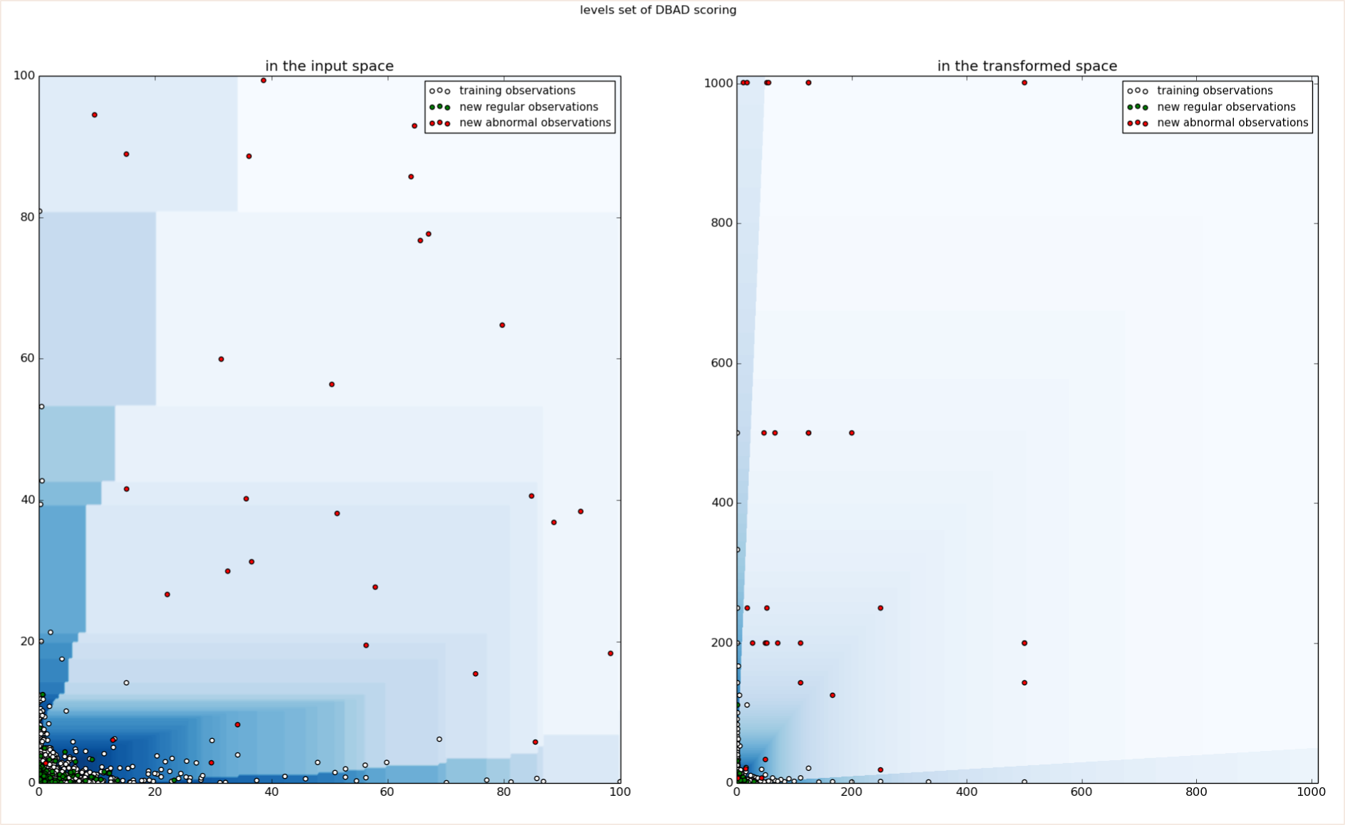
Figure 4: Level sets of $s_{n}$ on simulated 2D data

This heuristic argument explains the following algorithm, referred to as Detecting Anomaly with Multivariate EXtremes (DAMEX in abbreviated form). Note that this is a slightly modified version of the original DAMEX algorihtm empirically tested in Goix et al. (2016), where $\epsilon$-thickened sub-cones instead of $\epsilon$-thickened rectangles are considered. The proof is more straightforward when considering rectangles and performance remains as good. The complexity is in $O(dn\log n+dn)=O(dn\log n)$, where the first term on the left-hand-side comes from computing the $\widehat{F}_{j}(X_{i}^{j})$ (Step 1) by sorting the data (e.g. merge sort). The second one arises from Step 2.

Algorithm 1.

(DAMEX)
Input: parameters $\epsilon>0$,   $k=k(n)$,   $p\geq 0$. 1. Standardize via marginal rank-transformation: $\mathbf{\widehat{V}}_{i}:=\big{(}1/(1-\widehat{F}_{j}(X_{i}^{j}))\big{)}_{j=1,\ldots,d}$ . 2. Assign to each $\mathbf{\widehat{V}}_{i}$ the cone $R_{\alpha}^{\epsilon}$ it belongs to. 3. Compute $\widehat{\mathcal{M}}(\alpha)$ from (4.1) $\rightarrow$ yields: (small number of) cones with non-zero mass. 4. (Optional) Set to $0$ the $\widehat{\mathcal{M}}(\alpha)$ below some small threshold defined in remark 4 w.r.t. $p$.$\rightarrow$ yields: (sparse) representation of the dependence structure $\displaystyle\left\{\widehat{\mathcal{M}}(\alpha):\;\emptyset\alpha\subset\{1,\ldots,d\}\right\}.$ (4.4) Output: Compute the scoring function given by (4.3), $\displaystyle s_{n}(\mathbf{x}):=(1/\|\widehat{T}(\mathbf{x})\|_{\infty})\sum_{\alpha}\widehat{\mathcal{M}}(\alpha)\mathds{1}_{\widehat{T}(\mathbf{x})\in R_{\alpha}^{\epsilon}}.$

Before investigating how the algorithm above empirically performs when applied to synthetic/real datasets, a few remarks are in order.

Remark 6.

(Interpretation of the Parameters) In view of (4.1), $n/k$ is the threshold above which the data are considered as extreme and $k$ is proportional to the number of such data, a common approach in multivariate extremes. The tolerance parameter $\epsilon$ accounts for the non-asymptotic nature of data. The smaller $k$, the smaller $\epsilon$ shall be chosen. The additional angular mass threshold in step 4. acts as an additional sparsity inducing parameter. Note that even without this additional step (i.e. setting $p=0$, the obtained representation for real-world data (see Table 2) is already sparse (the number of charges cones is significantly less than $2^{d}$).

Remark 7.

(Choice of Parameters) A standard choice of parameters $(\epsilon,~{}k,~{}p)$ is respectively $(0.01,n^{1/2},0.1)$. However, there is no simple manner to choose optimally these parameters, as there is no simple way to determine how fast is the convergence to the (asymptotic) extreme behavior –namely how far in the tail appears the asymptotic dependence structure. Indeed, even though the first term of the error bound in Theorem 1 is proportional, up to re-scaling, to $\sqrt{\frac{1}{\epsilon k}}+\sqrt{\epsilon}$, which suggests choosing $\epsilon$ of order $k^{-1/4}$, the unknown bias term perturbs the analysis and in practice, one obtains better results with the values above mentioned. In a supervised or semi-supervised framework (or if a small labeled dataset is available) these three parameters should be chosen by cross-validation. In the unsupervised situation, a classical heuristic (Coles (2001)) is to choose $(k,\epsilon)$ in a stability region of the algorithm’s output: the largest $k$ (resp. the larger $\epsilon$) such that when decreased, the dependence structure remains stable. This amounts to selecting as many data as possible as being extreme (resp. in low dimensional regions), within a stability domain of the estimates, which exists under the primal assumption (2.1) and in view of Lemma 1.

Remark 8.

(Dimension Reduction) If the extreme dependence structure is low dimensional, namely concentrated on low dimensional cones $\mathcal{C}_{\alpha}$ – or in other terms if only a limited number of margins can be large together – then most of the $\widehat{V}_{i}$’s will be concentrated on the $R_{\alpha}^{\epsilon}$’s such that $|\alpha|$ (the dimension of the cone $\mathcal{C}_{\alpha}$) is small; then the representation of the dependence structure in (4.4) is both sparse and low dimensional.

Remark 9.

(Scaling Invariance) DAMEX produces the same result if the input data are transformed in such a way that the marginal order is preserved. In particular, any marginally increasing transform or any scaling as a preprocessing step does not affect the algorithm. It also implies invariance with respect to any change in the measuring units. This invariance property constitutes part of the strengh of the algorithm, since data preprocessing steps usually have a great impact on the overall performance and are of major concern in pratice.

5 Experimental results

5.1 Recovering the support of the dependence structure of generated data

Datasets of size $50000$ (respectively $100000$, $150000$) are generated in $\mathbb{R}^{10}$ according to a popular multivariate extreme value model, introduced by Tawn (1990), namely a multivariate asymmetric logistic distribution ($G_{log}$). The data have the following features: (i) they resemble ‘real life’ data, that is, the $X_{i}^{j}$’s are non zero and the transformed $\hat{V}_{i}$’s belong to the interior cone $\mathcal{C}_{\{1,\ldots,d\}}$, (ii) the associated (asymptotic) exponent measure concentrates on $K$ disjoint cones $\{\mathcal{C}_{\alpha_{m}},1\leq m\leq K\}$. For the sake of reproducibility, $G_{log}(\mathbf{x})=\exp\{-\sum_{m=1}^{K}\left(\sum_{j\in\alpha_{m}}(|A(j)|x_{j})^{-1/{w_{\alpha_{m}}}}\right)^{w_{\alpha_{m}}}\},$ where $|A(j)|$ is the cardinal of the set $\{\alpha\in D:j\in\alpha\}$ and where $w_{\alpha_{m}}=0.1$ is a dependence parameter (strong dependence). The data are simulated using Algorithm 2.2 in Stephenson (2003). The subset of sub-cones $D$ charged by $\mu$ is randomly chosen (for each fixed number of sub-cones $K$) and the purpose is to recover $D$ by Algorithm 1. For each $K$, $100$ experiments are made and we consider the number of ‘errors’, that is, the number of non-recovered or false-discovered sub-cones. Table 1 shows the averaged numbers of errors among the $100$ experiments.

$\#$ sub-cones $K$	3	5	10	15	20	25	30	35	40	45	50
Aver. $\#$ errors	0.02	0.65	0.95	0.45	0.49	1.35	4.19	8.9	15.46	19.92	18.99
(n=5e4)
Aver. $\#$ errors	0.00	0.45	0.36	0.21	0.13	0.43	0.38	0.55	1.91	1.67	2.37
(n=10e4)
Aver. $\#$ errors	0.00	0.34	0.47	0.00	0.02	0.13	0.13	0.31	0.39	0.59	1.77
(n=15e4)

Table 1: Support recovering on simulated data

The results are very promising in situations where the number of sub-cones is moderate w.r.t. the number of observations.

5.2 Sparse structure of extremes (wave data)

Our goal is here to verify that the two expected phenomena mentioned in the introduction, 1- sparse dependence structure of extremes (small number of sub-cones with non zero mass), 2- low dimension of the sub-cones with non-zero mass, do occur with real data. We consider wave directions data provided by Shell, which consist of $58585$ measurements $D_{i}$, $i\leq 58595$ of wave directions between $0^{\circ}$ and $360^{\circ}$ at $50$ different locations (buoys in North sea). The dimension is thus $50$. The angle $90^{\circ}$ being fairly rare, we work with data obtained as $X_{i}^{j}=1/(10^{-10}+|90-D_{i}^{j}|)$, where $D_{i}^{j}$ is the wave direction at buoy $j$, time $i$. Thus, $D_{i}^{j}$’s close to $90$ correspond to extreme $X_{i}^{j}$’s. Results in Table 2show that the number of sub-cones $\mathcal{C}_{\alpha}$ identified by Algorithm 1 is indeed small compared to the total number of sub-cones ($2^{50}$-1). (Phenomenon 1 in the introduction section). Further, the dimension of these sub-cones is essentially moderate (Phenomenon 2): respectively $93\%$, $98.6\%$ and $99.6\%$ of the mass is affected to sub-cones of dimension no greater than $10$, $15$ and $20$ respectively (to be compared with $d=50$). Histograms displaying the mass repartition produced by Algorithm 1 are given in Fig. 5.

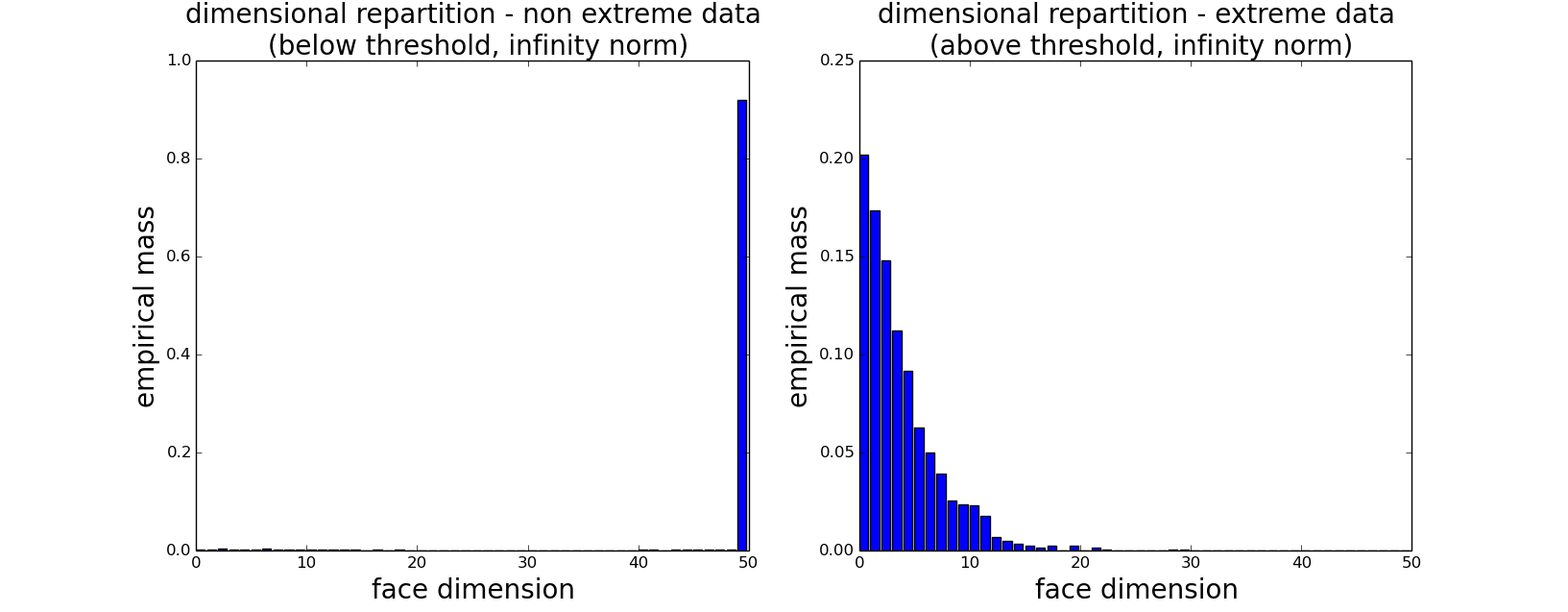
Figure 5: sub-cone dimensions of wave data

	non-extreme data	extreme data
nb of sub-cones with mass $>0$ ($p=0$)	3413	858
idem after thresholding ($p=0.1$)	2	64
idem after thresholding ($p=0.2$)	1	18

Table 2: Total number of sub-cones of wave data

5.3 Application to Anomaly Detection on real-world data sets

The main purpose of Algorithm 1 is to build a ‘normal profile’ for extreme data, so as to distinguish between normal and ab-normal extremes. In this section we evaluate its performance and compare it with that of a standard AD algorithm, the Isolation Forest (iForest) algorithm, which we chose in view of its established high performance (Liu et al. (2008)). The two algorithms are trained and tested on the same datasets, the test set being restricted to an extreme region. Five reference AD datasets are considered: shuttle, forestcover, http, SF and SA . The experiments are performed in a semi-supervised framework (the training set consists of normal data).

The shuttle dataset is the fusion of the training and testing datasets available in the UCI repository Lichman (2013). The data have $9$ numerical attributes, the first one being time. Labels from $7$ different classes are also available. Class $1$ instances are considered as normal, the others as anomalies. We use instances from all different classes but class $4$, which yields an anomaly ratio (class 1) of $7.17\%$.

In the forestcover data, also available at UCI repository (Lichman (2013)), the normal data are the instances from class $2$ while instances from class $4$ are anomalies, other classes are omitted, so that the anomaly ratio for this dataset is $0.9\%$.

The last three datasets belong to the KDD Cup ’99 dataset (KDDCup (1999), Tavallaee et al. (2009)), produced by processing the tcpdump portions of the 1998 DARPA Intrusion Detection System (IDS) Evaluation dataset, created by MIT Lincoln Lab Lippmann et al. (2000). The artificial data was generated using a closed network and a wide variety of hand-injected attacks (anomalies) to produce a large number of different types of attack with normal activity in the background. Since the original demonstrative purpose of the dataset concerns supervised AD, the anomaly rate is very high ($80\%$), which is unrealistic in practice, and inappropriate for evaluating the performance on realistic data. We thus take standard pre-processing steps in order to work with smaller anomaly rates. For datasets SF and http we proceed as described in Yamanishi et al. (2000): SF is obtained by picking up the data with positive logged-in attribute, and focusing on the intrusion attack, which gives an anomaly proportion of $0.48\%.$ The dataset http is a subset of SF corresponding to a third feature equal to ’http’. Finally, the SA dataset is obtained as in Eskin et al. (2002) by selecting all the normal data, together with a small proportion ($1\%$) of anomalies.

Table 3 summarizes the characteristics of these datasets. The thresholding parameter $p$ is fixed to $0.1$, the averaged mass of the non-empty sub-cones, while the parameters $(k,\epsilon)$ are standardly chosen as $(n^{1/2},0.01)$. The extreme region on which the evaluation step is performed is chosen as $\{\mathbf{x}:~{}\|T(\mathbf{x})\|>\sqrt{n}\}$, where $n$ is the training set’s sample size. The ROC and PR curves are computed using only observations in the extreme region. This provides a precise evaluation of the two AD methods on extreme data. For each of them, 20 experiments on random training and testing datasets are performed, yielding averaged ROC and Precision-Recall curves whose AUC are presented in Table 4. DAMEX significantly improves the performance (both in term of precision and of ROC curves) in extreme regions for each dataset, as illustrated in figures 6 and 7.

In Table 5, we repeat the same experiments but with $\epsilon=0.1$. This yields the same strong performance of DAMEX, excepting for SF. Generally, to large $\epsilon$ may yield over-estimated $\widehat{\mathcal{M}}(\alpha)$ for low-dimensional faces $\alpha$. Such a performance gap between $\epsilon=0.01$ and $\epsilon=0.1$ can also be explained by the fact that anomalies may form a cluster which is wrongly include in some over-estimated ‘normal’ sub-cone, when $\epsilon$ is too large. Such singular anomaly structure would also explain the counter performance of iForest on this dataset.

We also point out that for very small values of epsilon ($\epsilon\leq 0.001$), the performance of DAMEX significantly decreases on these datasets. With such a small $\epsilon$, most observations belong to the central cone (the one of dimension $d$) which is widely over-estimated, while the other cones are under-estimated.

The only case were using very small $\epsilon$ should be useful, is when the asymptotic behaviour is clearly reached at level $k$ (usually for very large threshold $n/k$, e.g. $k=n^{1/3}$), or in the specific case where anomalies clearly concentrate in low dimensional sub-cones: The use of a small $\epsilon$ precisely allows to assign a high abnormality score to these subcones (under-estimation of the asymptotic mass), which yields better performances.

The averaged ROC curves and PR curves for the other datasets are gathered in B.

	shuttle	forestcover	SA	SF	http
Samples total	85849	286048	976158	699691	619052
Number of features	9	54	41	4	3
Percentage of anomalies	7.17	0.96	0.35	0.48	0.39

Table 3: Datasets characteristics

Dataset	iForest		DAMEX
	AUC ROC	AUC PR	AUC ROC	AUC PR
shuttle	0.957	0.987	$\mathbf{0.988}$	$\mathbf{0.996}$
forestcover	0.667	0.201	$\mathbf{0.976}$	$\mathbf{0.805}$
http	0.561	0.321	$\mathbf{0.981}$	$\mathbf{0.742}$
SF	0.134	0.189	$\mathbf{0.988}$	$\mathbf{0.973}$
SA	0.932	0.625	$\mathbf{0.945}$	$\mathbf{0.818}$

Table 4: Results on extreme regions with standard parameters $(k,\epsilon)=(n^{1/2},0.01)$

Dataset	iForest		DAMEX
	AUC ROC	AUC PR	AUC ROC	AUC PR
shuttle	0.957	0.987	$\mathbf{0.980}$	$\mathbf{0.995}$
forestcover	0.667	0.201	$\mathbf{0.984}$	$\mathbf{0.852}$
http	0.561	0.321	$\mathbf{0.971}$	$\mathbf{0.639}$
SF	$\mathbf{0.134}$	0.189	0.101	$\mathbf{0.211}$
SA	0.932	0.625	$\mathbf{0.964}$	$\mathbf{0.848}$

Table 5: Results on extreme regions with lower $\epsilon=0.1$

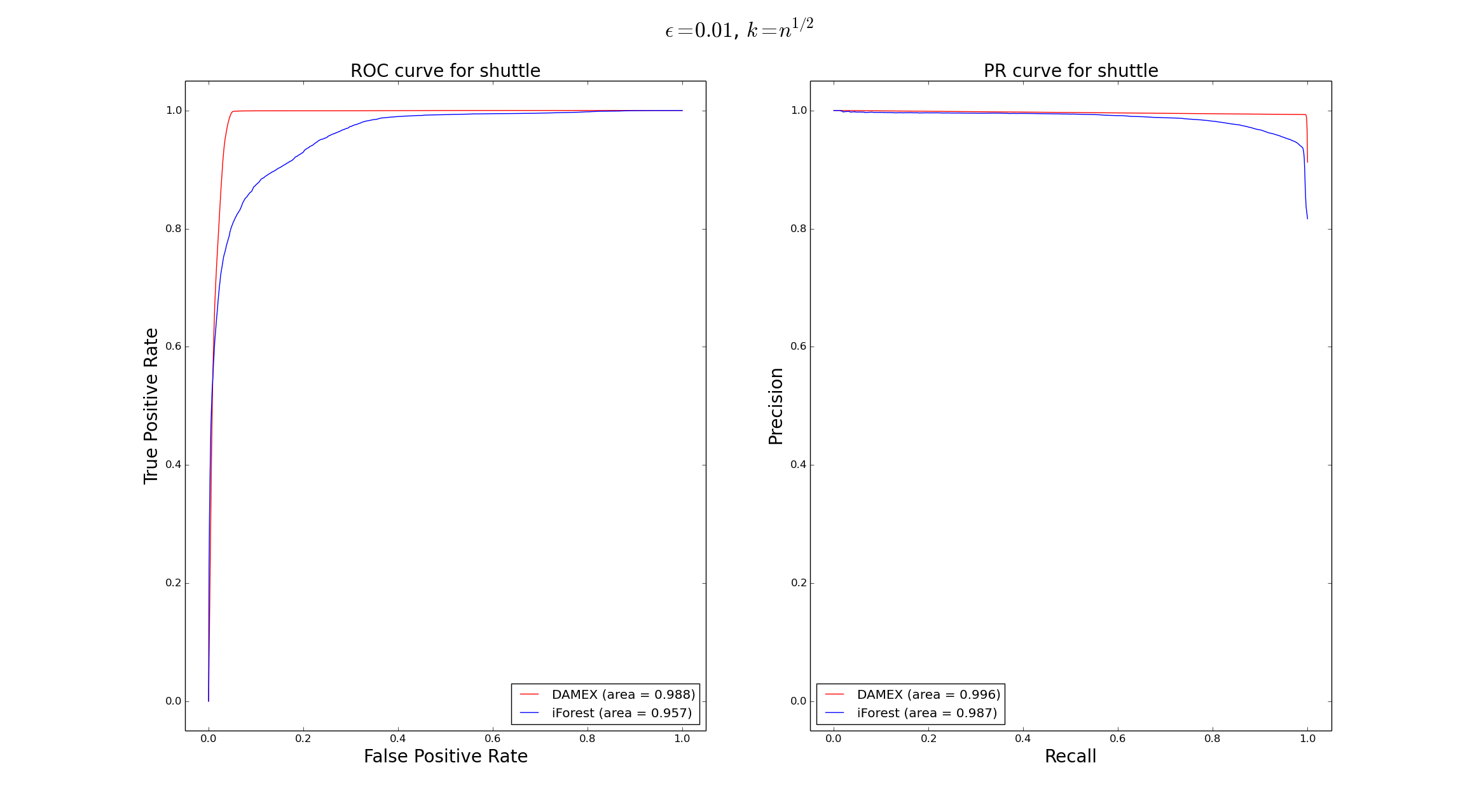
Figure 6: SF dataset, default parameters

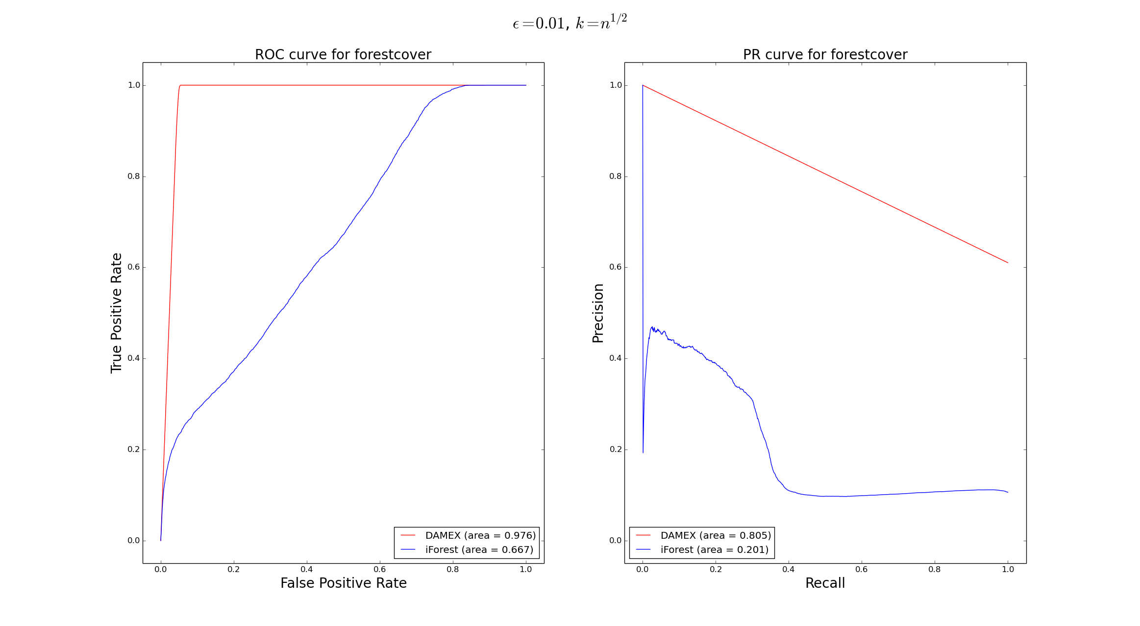
Figure 7: SF dataset, larger $\epsilon$

Considering the significant performance improvements on extreme data, DAMEX may be combined with any standard AD algorithm to handle extreme and non-extreme data. This would improve the global performance of the chosen standard algorithm, and in particular decrease the false alarm rate (increase the slope of the ROC curve’s tangents near the origin). This combination can be done by splitting the input space between an extreme region and a non-extreme one, then using Algorithm 1 to treat new observations that appear in the extreme region, and the standard algorithm to deal with those which appear in the non-extreme region.

6 Conclusion

The contribution of this work is twofold. First, it brings advances in multivariate EVT by designing a statistical method that possibly exhibits a sparsity pattern in the dependence structure of extremes, while deriving non-asymptotic bounds to assess the accuracy of the estimation procedure. Our method is intended to be used as a preprocessing step to scale up multivariate extreme values modeling to high dimensional settings, which is currently one of the major challenges in multivariate EVT. Since the asymptotic bias ($\text{bias}(\alpha,n,k,\epsilon)$ in eq. (3.21)) appears as a separate term in the bound established, no second order assumption is required. One possible line of further research would be to make such an assumption (i.e. to assume that the bias itself is regularly varying), in order to choose $\epsilon$ adaptively with respect to $k$ and $n$ (see Remark 7). This might also open up the possibility of de-biasing the estimation procedure (Fougeres et al. (2015), Beirlant et al. (2015)). As a second contribution, this work extends the applicability of multivariate EVT to the field of Anomaly Detection: a multivariate EVT-based algorithm which scores extreme observations according to their degree of abnormality is proposed. Due to its moderate complexity –of order $dn\log n$– this algorithm is suitable for the treatment of real word large-scale learning problems, and experimental results reveal a significantly increased performance on extreme regions compared with standard AD approaches.

Appendix A Technical proofs

A.1 Proof of Lemma 3

For $n$ vectors $\mathbf{v}_{1},\ldots,\mathbf{v}_{n}$ in $\mathbb{R}^{d}$, let us denote by $rank(v_{i}^{j})$ the rank of $v_{i}^{j}$ among $v_{1}^{j},\ldots,v_{n}^{j}$, that is $rank(v_{i}^{j})=\sum_{k=1}^{n}\mathds{1}_{\{v_{k}^{j}\leq v_{i}^{j}\}}$, so that $\hat{F}_{j}(X_{i}^{j})=(rank(X_{i}^{j})-1)/n$. For the first equivalence, notice that $\hat{V}_{i}^{j}=1/\hat{U}_{i}^{j}$. For the others, we have both at the same time:

$$\hat{V}_{i}^{j}\geq\frac{n}{k}x_{j} ~{}~{}\Leftrightarrow~{}~{}1-\frac{rank(X_{i}^{j})-1}{n}~{}\leq~{}\frac{k}{n}~{}x_{j}^{-1}$$

$$~{}~{}\Leftrightarrow~{}~{}rank(X_{i}^{j})\geq n-kx_{j}^{-1}+1$$

$$~{}~{}\Leftrightarrow~{}~{}rank(X_{i}^{j})\geq n-\lfloor kx_{j}^{-1}\rfloor+1$$

$$~{}~{}\Leftrightarrow~{}~{}X_{i}^{j}\geq X_{(n-\lfloor kx_{j}^{-1}\rfloor+1)}^{j},$$

and

$$X_{i}^{j}\geq X_{(n-\lfloor kx_{j}^{-1}\rfloor+1)}^{j}~{}\Leftrightarrow~{}rank(X_{i}^{j})\geq n-\lfloor kx_{j}^{-1}\rfloor+1$$

$$~{}~{}~{}~{}~{}~{}~{}~{}~{}~{}~{}~{}~{}~{}~{}~{}\Leftrightarrow~{}rank(F_{j}(X_{i}^{j}))\geq n-\lfloor kx_{j}^{-1}\rfloor+1\qquad(\text{with probability one})$$

$$~{}~{}~{}~{}~{}~{}~{}~{}~{}~{}~{}~{}~{}~{}~{}~{}\Leftrightarrow~{}rank(1-F_{j}(X_{i}^{j}))\leq\lfloor kx_{j}^{-1}\rfloor$$

$$~{}~{}~{}~{}~{}~{}~{}~{}~{}~{}~{}~{}~{}~{}~{}~{}\Leftrightarrow~{}U_{i}^{j}\leq U_{(\lfloor kx_{j}^{-1}\rfloor)}^{j}.$$

A.2 Proof of Lemma 4

First, recall that $g_{\alpha,\beta}(\mathbf{x},\mathbf{z})=\mu\big{(}R(\mathbf{x}^{-1},\mathbf{z}^{-1},\alpha,\beta)\big{)}$, see (3.13). Denote by $\pi$ the transformation to pseudo-polar coordinates introduced in Section 2,

$$\pi:[0,\infty]^{d}\setminus\{\mathbf{0}\} \to(0,\infty]\times S^{d-1}_{\infty}$$

$$\mathbf{v} \mapsto(r,\boldsymbol{\theta})=(\|\mathbf{v}\|_{\infty},\|\mathbf{v}\|_{\infty}^{-1}\mathbf{v}).$$

Then, we have $\mathrm{d}(\mu\circ\pi^{-1})=\frac{\mathrm{d}r}{r^{2}}\mathrm{d}\Phi$ on $(0,\infty]\times S^{d-1}_{\infty}$. This classical result from EVT comes from the fact that, for $r_{0}>0$ and $B\subset S^{d-1}_{\infty}$, $\mu\circ\pi^{-1}\{r\geq r_{0},\boldsymbol{\theta}\in B\}=r_{0}^{-1}\Phi(B)$, see (2.6). Then

$$g_{\alpha,\beta}(\mathbf{x},\mathbf{z}) =\mu\circ\pi^{-1}\Big{\{}(r,\boldsymbol{\theta}):\quad\forall i\in\alpha,~{}r\theta_{i}\geq x_{i}^{-1}\;;\quad\forall j\in\beta,r\theta_{j}<z_{j}^{-1}\Big{\}}$$

$$=\mu\circ\pi^{-1}\Big{\{}(r,\boldsymbol{\theta}):\quad r\geq\bigvee_{i\in\alpha}(\theta_{i}x_{i})^{-1}\;;\quad r<\bigwedge_{j\in\beta}(\theta_{j}z_{j})^{-1}\Big{\}}$$

$$=\int_{\boldsymbol{\theta}\in S^{d-1}_{\infty}}\int_{r>0}\mathds{1}_{r\geq\bigvee_{i\in\alpha}(\theta_{i}x_{i})^{-1}}\;\mathds{1}_{r<\bigwedge_{j\in\beta}(\theta_{j}z_{j})^{-1}}\frac{\mathrm{d}r}{r^{2}}\mathrm{d}\Phi(\boldsymbol{\theta})$$

$$=\int_{\boldsymbol{\theta}\in S^{d-1}_{\infty}}\left(\Big{(}\bigvee_{i\in\alpha}(\theta_{i}x_{i})^{-1}\Big{)}^{-1}-\Big{(}\bigwedge_{j\in\beta}(\theta_{j}z_{j})^{-1}\Big{)}^{-1}\right)_{+}\mathrm{d}\Phi(\boldsymbol{\theta})$$

$$=\int_{\boldsymbol{\theta}\in S^{d-1}_{\infty}}\left(\bigwedge_{i\in\alpha}\theta_{i}x_{i}-\bigvee_{j\in\beta}\theta_{j}z_{j}\right)_{+}\mathrm{d}\Phi(\boldsymbol{\theta}),$$

which proves the first assertion. To prove the Lipschitz property, notice first that, for any finite sequence of real numbers $c$ and $d$, $\max_{i}c_{i}-\max_{i}d_{i}\leq\max_{i}(c_{i}-d_{i})$ and $\min_{i}c_{i}-\min_{i}d_{i}\leq\max_{i}(c_{i}-d_{i})$. Thus for every $\mathbf{x},\mathbf{z}\in[0,\infty]^{d}\setminus\{\boldsymbol{\infty}\}$ and $\theta\in S_{\infty}^{d-1}$:

$$\left(\bigwedge_{j\in\alpha}{\theta_{j}x_{j}}-\bigvee_{j\in\beta}\theta_{j}z_{j}\right)_{+}-\left(\bigwedge_{j\in\alpha}{\theta_{j}x_{j}^{\prime}}-\bigvee_{j\in\beta}\theta_{j}z_{j}^{\prime}\right)_{+}$$

$$~{}~{}~{}~{}~{}~{}~{}~{}~{}~{}~{}~{}~{}~{}~{}~{}~{}~{}~{}~{}~{}~{}~{}~{}~{}~{}~{}~{}\leq~{}\left[\left(\bigwedge_{j\in\alpha}{\theta_{j}x_{j}}-\bigvee_{j\in\beta}\theta_{j}z_{j}\right)-\left(\bigwedge_{j\in\alpha}{\theta_{j}x_{j}^{\prime}}-\bigvee_{j\in\beta}\theta_{j}z_{j}^{\prime}\right)\right]_{+}$$

$$~{}~{}~{}~{}~{}~{}~{}~{}~{}~{}~{}~{}~{}~{}~{}~{}~{}~{}~{}~{}~{}~{}~{}~{}~{}~{}~{}~{}\leq~{}\left[\bigwedge_{j\in\alpha}{\theta_{j}x_{j}}-\bigwedge_{j\in\alpha}{\theta_{j}x_{j}^{\prime}}~{}+~{}\bigvee_{j\in\beta}\theta_{j}z_{j}^{\prime}-\bigvee_{j\in\beta}\theta_{j}z_{j}\right]_{+}$$

$$~{}~{}~{}~{}~{}~{}~{}~{}~{}~{}~{}~{}~{}~{}~{}~{}~{}~{}~{}~{}~{}~{}~{}~{}~{}~{}~{}~{}\leq~{}\left[\max_{j\in\alpha}(\theta_{j}x_{j}-\theta_{j}x_{j}^{\prime})~{}+~{}\max_{j\in\beta}(\theta_{j}z_{j}^{\prime}-\theta_{j}z_{j})\right]_{+}$$

$$~{}~{}~{}~{}~{}~{}~{}~{}~{}~{}~{}~{}~{}~{}~{}~{}~{}~{}~{}~{}~{}~{}~{}~{}~{}~{}~{}~{}\leq~{}\max_{j\in\alpha}\theta_{j}|{x_{j}}-{x_{j}^{\prime}}|~{}+~{}\max_{j\in\beta}\theta_{j}|z_{j}^{\prime}-z_{j}|$$

Hence,

$$|g_{\alpha,\beta}(\mathbf{x},\mathbf{z})-g_{\alpha,\beta}(\mathbf{x}^{\prime},\mathbf{z}^{\prime})|$$

$$~{}~{}~{}~{}~{}~{}~{}~{}~{}~{}~{}~{}~{}~{}~{}~{}~{}~{}~{}~{}~{}~{}~{}\leq~{}\int_{S^{d-1}_{\infty}}\left(\max_{j\in\alpha}\theta_{j}|{x_{j}}-{x_{j}^{\prime}}|~{}+~{}\max_{j\in\beta}\theta_{j}|z_{j}^{\prime}-z_{j}|\right)\mathrm{d}\Phi(\boldsymbol{\theta})~{}.$$

Now, by (2.7) we have:

$$\int_{S^{d-1}_{\infty}}\max_{j\in\alpha}\theta_{j}|{x_{j}}-{x_{j}^{\prime}}|~{}~{}\mathrm{d}\Phi(\boldsymbol{\theta})=\mu([\mathbf{0},\mathbf{\tilde{x}}^{-1}]^{c})$$

with $\mathbf{\tilde{x}}$ defined as $\tilde{x}_{j}=|x_{j}-x_{j}^{\prime}|$ for $j\in\alpha$, and $0$ elsewhere. It suffices then to write:

$$\mu([\mathbf{0},\mathbf{\tilde{x}}^{-1}]^{c}) =\mu(\{y,~{}\exists j\in\alpha,~{}y_{j}\geq|x_{j}-x_{j}^{\prime}|^{-1}\})$$

$$\leq\sum_{j\in\alpha}\mu(\{y,~{}y_{j}\geq|x_{j}-x_{j}^{\prime}|^{-1}\})$$

$$\leq\sum_{j\in\alpha}|x_{j}-x_{j}^{\prime}|~{}.$$

Similarly, $\int_{S^{d-1}_{\infty}}\max_{j\in\beta}\theta_{j}|z_{j}^{\prime}-z_{j}|~{}~{}\mathrm{d}\Phi(\boldsymbol{\theta})~{}\leq~{}\sum_{j\in\beta}|z_{j}-z_{j}^{\prime}|$.

A.3 Proof of Proposition 1

The starting point is inequality (9) on p.7 in Goix et al. (2015) which bounds the deviation of the empirical measure on extreme regions. Let $\mathcal{C}_{n}(\,\cdot\,)=\frac{1}{n}\sum_{i=1}^{n}\mathds{1}_{\{\mathbf{Z}_{i}\in\,\cdot\,\}}$ and $\mathcal{C}(\mathbf{x})=\mathbb{P}(\mathbf{Z}\in\,\cdot\,)$ be the empirical and true measures associated with a n-sample $\mathbf{Z}_{1},\ldots,\mathbf{Z}_{d}$ of $\mathit{i.i.d.}$  realizations of a random vector $\mathbf{Z}=(Z^{1},\ldots,Z^{d})$ with uniform margins on $[0,1]$. Then for any real number $\delta\geq e^{-k}$, with probability greater than $1-\delta$,

$$\sup_{0\leq\mathbf{x}\leq T}\frac{n}{k}\left|\mathcal{C}_{n}(\frac{k}{n}[\mathbf{x},\boldsymbol{\infty}[^{c})-\mathcal{C}(\frac{k}{n}[\mathbf{x},\boldsymbol{\infty}[^{c})\right|~{}\leq~{}Cd\sqrt{\frac{T}{k}\log{\frac{1}{\delta}}}~{}.$$ (A.1)

Recall that with the above notations, $0\leq\mathbf{x}\leq T$ means $0\leq x_{j}\leq T$ for every $j$. The proof of Proposition 1 follows the same lines as in Goix et al. (2015). The cornerstone concentration inequality (A.1) has to be replaced with

$$\max_{\alpha,\beta}\sup_{\begin{subarray}{c}0\leq\mathbf{x},\mathbf{z}\leq T\\ \exists j\in\alpha,x_{j}\leq T^{\prime}\end{subarray}} \frac{n}{k}\left|\mathcal{C}_{n}\left(\frac{k}{n}R(\mathbf{x}^{-1},\mathbf{z}^{-1},\alpha,~{}\beta)^{-1}\right)-\mathcal{C}\left(\frac{k}{n}R(\mathbf{x}^{-1},\mathbf{z}^{-1},\alpha,~{}\beta)^{-1}\right)\right|$$

$$~{}~{}~{}~{}~{}~{}~{}~{}~{}~{}~{}~{}~{}~{}~{}~{}~{}~{}~{}~{}~{}~{}~{}~{}~{}~{}~{}~{}~{}~{}~{}~{}~{}~{}~{}~{}~{}~{}~{}~{}~{}~{}\leq~{}Cd\sqrt{\frac{dT^{\prime}}{k}\log{\frac{1}{\delta}}}~{}.$$ (A.2)

Remark 10.

Inequality (A.3) is here written in its full generality, namely with a separate constant $T^{\prime}$ possibly smaller than $T$. If $T^{\prime}<T$, we then have a smaller bound (typically, we may use $T=1/\epsilon$ and $T^{\prime}=1$). However, we only use (A.3) with $T=T^{\prime}$ in the analysis below, since the smaller bounds in $T^{\prime}$ obtained (on $\Lambda(n)$ in (A.5)) would be diluted (by $\Upsilon(n)$ in (A.5)).

Proof of (A.3).

Recall that for notational convenience we write ‘$\alpha,\beta$’ for ‘$\alpha$ non-empty subset of $\{1,\ldots,d\}$ and $\beta$ subset of $\{1,\ldots,d\}$’. The key is to apply Theorem 1 in Goix et al. (2015), with a VC-class which fits our purposes. Namely, consider

$$\mathcal{A}~{}~{}=~{}~{}\mathcal{A}_{T,T^{\prime}}~{}~{} =~{}~{}\bigcup_{\alpha,\beta}\mathcal{A}_{T,T^{\prime},\alpha,\beta}\text{~{}~{}~{}~{}~{}with}$$

$$\mathcal{A}_{T,T^{\prime},\alpha,\beta}~{}~{}=~{}~{} \frac{k}{n}\Big{\{}R(\mathbf{x}^{-1},\mathbf{z}^{-1},\alpha,~{}\beta)^{-1}:~{}~{}\mathbf{x},\mathbf{z}\in\mathbb{R}^{d},~{}0\leq\mathbf{x},\mathbf{z}\leq T,$$

$$~{}~{}~{}~{}~{}~{}~{}~{}~{}~{}~{}~{}~{}~{}~{}~{}~{}~{}~{}~{}~{}~{}~{}~{}~{}~{}~{}~{}~{}~{}~{}~{}~{}~{}~{}~{}~{}~{}~{}~{}~{}~{}~{}~{}~{}~{}~{}~{}~{}~{}~{}~{}~{}~{}~{}~{}\exists j\in\alpha,x_{j}\leq T^{\prime}\Big{\}}~{},$$

for $T,~{}T^{\prime}>0$ and $\alpha,~{}\beta\subset\{1,\ldots,d\},~{}\alpha\neq\emptyset$. $\mathcal{A}$ has VC-dimension $V_{\mathcal{A}}=d$, as the one considered in Goix et al. (2015). Recall in view of (3.10) that

$$R(\mathbf{x}^{-1},\mathbf{z}^{-1},\alpha,~{}\beta)^{-1}~{} =~{}\Big{\{}\mathbf{y}\in[0,\infty]^{d},~{}~{}y_{j}\leq x_{j}~{}~{}\text{ for }j\in\alpha,$$

$$~{}~{}~{}~{}~{}~{}~{}~{}~{}~{}~{}~{}~{}~{}~{}~{}~{}~{}~{}~{}~{}~{}~{}~{}~{}y_{j}>z_{j}~{}~{}\text{ for }j\in\beta~{}~{}\Big{\}}$$

$$=~{}[\mathbf{a},\mathbf{b}],$$

with $\mathbf{a}$ and $\mathbf{b}$ defined by $a_{j}=\left\{\begin{array}[]{cc}0&\text{for}~{}j\in\alpha\\ z_{j}&\text{for}~{}j\in\beta\\ \end{array}\right.$ and $b_{j}=\left\{\begin{array}[]{cc}x_{j}&\text{for}~{}j\in\alpha\\ \infty&\text{for}~{}j\in\beta\\ \end{array}\right.$. Since we have $\forall A\in\mathcal{A},A\subset[\frac{k}{n}\mathbf{T}^{\prime},~{}\boldsymbol{\infty}[^{c}$, the probability for a r.v. $\mathbf{Z}$ with uniform margins in $[0,1]$ to be in the union class $\mathbb{A}=\bigcup_{A\in\mathcal{A}}A$ is $\mathbb{P}(\mathbf{Z}\in\mathbb{A})\leq\mathbb{P}(\mathbf{Z}\in[\frac{k}{n}\mathbf{T}^{\prime},~{}\boldsymbol{\infty}[^{c})\leq\sum_{j=1}^{d}\mathbb{P}(Z^{j}\leq\frac{k}{n}T^{\prime})\leq\frac{k}{n}dT^{\prime}$. Inequality (A.3) is thus a direct consequence of Theorem 1 in Goix et al. (2015). ∎

Define now the empirical version $\tilde{F}_{n,\alpha,\beta}$ of $\tilde{F}_{\alpha,\beta}$ (introduced in (3.12)) as

$$\tilde{F}_{n,\alpha,\beta}(\mathbf{x},\mathbf{z})~{}=~{}\frac{1}{n}\sum_{i=1}^{n}\mathds{1}_{\{U_{i}^{j}\leq x_{j}~{}~{}\text{for}~{}j\in\alpha~{}~{}\text{ and }~{}~{}U_{i}^{j}>z_{j}~{}~{}\text{for}~{}j\in\beta\}}~{},$$ (A.3)

so that $\frac{n}{k}\tilde{F}_{n,\alpha,\beta}(\frac{k}{n}\mathbf{x},\frac{k}{n}\mathbf{z})~{}=~{}\frac{1}{k}\sum_{i=1}^{n}\mathds{1}_{\{U_{i}^{j}\leq\frac{k}{n}x_{j}~{}~{}\text{for}~{}j\in\alpha~{}~{}\text{ and }~{}~{}U_{i}^{j}>\frac{k}{n}z_{j}~{}~{}\text{for}~{}j\in\beta\}}.$ Notice that the $U_{i}^{j}$’s are not observable (since $F_{j}$ is unknown). In fact, $\tilde{F}_{n,\alpha,\beta}$ will be used as a substitute for $g_{n,\alpha,\beta}$ (defined in (3.14)) allowing to handle uniform variables. This is illustrated by the following lemmas.

Lemma 6 (Link between $g_{n,\alpha,\beta}$ and $\tilde{F}_{n,\alpha,\beta}$).

The empirical version of $\tilde{F}_{\alpha,\beta}$ and that of $g_{\alpha,\beta}$ are related via

$$g_{n,\alpha,\beta}(\mathbf{x},\mathbf{z})~{}=~{}\frac{n}{k}\tilde{F}_{n,\alpha,\beta}\left(\left(U_{(\lfloor kx_{j}\rfloor)}^{j}\right)_{j\in\alpha},\left(U_{(\lfloor kz_{j}\rfloor)}^{j}\right)_{j\in\beta}\right),$$

Proof.

Considering the definition in (A.3) and (3.3), both sides are equal to $\mu_{n}(R(\mathbf{x}^{-1},\mathbf{z}^{-1},\alpha,\beta))$. ∎

Lemma 7 (Uniform bound on $\tilde{F}_{n,\alpha,\beta}$’s deviations).

For any finite $T>0$, and $\delta\geq e^{-k}$, with probability at least $1-\delta$, the deviation of $\tilde{F}_{n,\alpha,\beta}$ from $\tilde{F}_{\alpha,\beta}$ is uniformly bounded:

$$\max_{\alpha,\beta}\sup_{0\leq\mathbf{x},\mathbf{z}\leq T}\left|\frac{n}{k}\tilde{F}_{n,\alpha,\beta}(\frac{k}{n}\mathbf{x},\frac{k}{n}\mathbf{z})-\frac{n}{k}\tilde{F}_{\alpha,\beta}(\frac{k}{n}\mathbf{x},\frac{k}{n}\mathbf{z})\right|\leq Cd\sqrt{\frac{T}{k}\log{\frac{1}{\delta}}}~{}.$$

Proof.

Notice that

$$\sup_{0\leq\mathbf{x},\mathbf{z}\leq T}\left|\frac{n}{k}\tilde{F}_{n,\alpha,\beta}(\frac{k}{n}\mathbf{x},\frac{k}{n}\mathbf{z})-\frac{n}{k}\tilde{F}_{\alpha,\beta}(\frac{k}{n}\mathbf{x},\frac{k}{n}\mathbf{z})\right|$$

$$~{}=\sup_{0\leq\mathbf{x},\mathbf{z}\leq T}\frac{n}{k}\left|\frac{1}{n}\sum_{i=1}^{n}\mathds{1}_{\mathbf{U}_{i}\in\frac{k}{n}R(\mathbf{x}^{-1},\mathbf{z}^{-1},\alpha,~{}\beta)^{-1}}-\mathbb{P}\left[\mathbf{U}\in\frac{k}{n}R(\mathbf{x}^{-1},\mathbf{z}^{-1},\alpha,~{}\beta)^{-1}\right]\right|,$$

and apply inequality (A.3) with $T^{\prime}=T$. ∎

Remark 11.

Note that the following stronger inequality holds true, when using (A.3) in full generality, i.e. with $T^{\prime}<T$. For any finite $T,T^{\prime}>0$, and $\delta\geq e^{-k}$, with probability at least $1-\delta$,

$$\max_{\alpha,\beta}\sup_{\begin{subarray}{c}0\leq\mathbf{x},\mathbf{z}\leq T\\ \exists j\in\alpha,x_{j}\leq T^{\prime}\end{subarray}}\left|\frac{n}{k}\tilde{F}_{n,\alpha,\beta}(\frac{k}{n}\mathbf{x},\frac{k}{n}\mathbf{z})-\frac{n}{k}\tilde{F}_{\alpha,\beta}(\frac{k}{n}\mathbf{x},\frac{k}{n}\mathbf{z})\right|\leq Cd\sqrt{\frac{T^{\prime}}{k}\log{\frac{1}{\delta}}}.$$

The following lemma is stated and proved in Goix et al. (2015).

Lemma 8 (Bound on the order statistics of $\mathbf{U}$).

Let $\delta\geq e^{-k}$. For any finite positive number $T>0$ such that $T\geq 7/2((\log d)/k+1)$, we have with probability greater than $1-\delta$,

$$\forall~{}1\leq j\leq d,~{}~{}~{}~{}~{}\frac{n}{k}U_{(\lfloor kT\rfloor)}^{j}~{}\leq~{}2T~{},$$ (A.4)

and with probability greater than $1-(d+1)\delta$,

$$\max_{1\leq j\leq d}~{}\sup_{0\leq x_{j}\leq T}\left|\frac{\lfloor kx_{j}\rfloor}{k}-\frac{n}{k}U_{(\lfloor kx_{j}\rfloor)}^{j}\right|~{}\leq~{}C\sqrt{\frac{T}{k}\log{\frac{1}{\delta}}}~{}.$$

We may now proceed with the proof of Proposition 1. Using Lemma 6, we may write:

$$\max_{\alpha,\beta}\sup_{0\leq\mathbf{x},\mathbf{z}\leq T}\left|g_{n,\alpha,\beta}(\mathbf{x},\mathbf{z})-g_{\alpha,\beta}(\mathbf{x},\mathbf{z})\right|$$

$$~{}~{}~{}~{}~{}~{}~{}~{}~{}~{}=~{}\max_{\alpha,\beta}\sup_{0\leq\mathbf{x},\mathbf{z}\leq T}\left|\frac{n}{k}\tilde{F}_{n,\alpha,\beta}\left(\left(U_{(\lfloor kx_{j}\rfloor)}^{j}\right)_{j\in\alpha},\left(U_{(\lfloor kz_{j}\rfloor)}^{j}\right)_{j\in\beta}\right)-g_{\alpha,\beta}(\mathbf{x},\mathbf{z})\right|$$

$$~{}~{}~{}~{}~{}~{}~{}~{}~{}~{}\leq~{}\Lambda(n)~{}+~{}\Xi(n)~{}+~{}\Upsilon(n)~{}.$$ (A.5)

with:

$$\Lambda(n) ~{}=~{}\max_{\alpha,\beta}\sup_{0\leq\mathbf{x},\mathbf{z}\leq T}\bigg{|}\frac{n}{k}\tilde{F}_{n,\alpha,\beta}\left(\left(U_{(\lfloor kx_{j}\rfloor)}^{j}\right)_{j\in\alpha},\left(U_{(\lfloor kz_{j}\rfloor)}^{j}\right)_{j\in\beta}\right)$$

$$~{}~{}~{}~{}~{}~{}~{}~{}~{}~{}~{}~{}~{}~{}~{}~{}~{}~{}~{}~{}~{}~{}~{}~{}~{}~{}~{}~{}~{}~{}~{}~{}~{}~{}~{}~{}~{}~{}~{}-\frac{n}{k}\tilde{F}_{\alpha,\beta}\left(\left(U_{(\lfloor kx_{j}\rfloor)}^{j}\right)_{j\in\alpha},\left(U_{(\lfloor kz_{j}\rfloor)}^{j}\right)_{j\in\beta}\right)\bigg{|}$$

$$\Xi(n) ~{}=~{}\max_{\alpha,\beta}\sup_{0\leq\mathbf{x},\mathbf{z}\leq T}\bigg{|}\frac{n}{k}\tilde{F}_{\alpha,\beta}\left(\left(U_{(\lfloor kx_{j}\rfloor)}^{j}\right)_{j\in\alpha},\left(U_{(\lfloor kz_{j}\rfloor)}^{j}\right)_{j\in\beta}\right)$$

$$~{}~{}~{}~{}~{}~{}~{}~{}~{}~{}~{}~{}~{}~{}~{}~{}~{}~{}~{}~{}~{}~{}~{}~{}~{}~{}~{}~{}~{}~{}~{}~{}~{}~{}~{}~{}~{}-g_{\alpha,\beta}\left(\left(\frac{n}{k}U_{(\lfloor kx_{j}\rfloor)}^{j}\right)_{j\in\alpha},\left(\frac{n}{k}U_{(\lfloor kz_{j}\rfloor)}^{j}\right)_{j\in\beta}\right)\bigg{|}$$

$$\Upsilon(n) ~{}=~{}\max_{\alpha,\beta}\sup_{0\leq\mathbf{x},\mathbf{z}\leq T}\left|g_{\alpha,\beta}\left(\left(\frac{n}{k}U_{(\lfloor kx_{j}\rfloor)}^{j}\right)_{j\in\alpha},\left(\frac{n}{k}U_{(\lfloor kz_{j}\rfloor)}^{j}\right)_{j\in\beta}\right)-g_{\alpha,\beta}(\mathbf{x},\mathbf{z})\right|.$$

Now, considering (A.4) we have with probability greater than $1-\delta$ that for every $1\leq j\leq d$, $U_{(\lfloor kT\rfloor)}^{j}~{}\leq~{}2T\frac{k}{n}~{}$, so that

$$\Lambda(n)~{}\leq~{}\max_{\alpha,\beta}\sup_{0\leq\mathbf{x},\mathbf{z}\leq 2T}\left|\frac{n}{k}\tilde{F}_{n,\alpha,\beta}\left(\frac{k}{n}\mathbf{x},\frac{k}{n}\mathbf{z}\right)-\frac{n}{k}\tilde{F}_{\alpha,\beta}\left(\frac{k}{n}\mathbf{x},\frac{k}{n}\mathbf{z}\right)\right|.$$

Thus by Lemma 7, with probability at least $1-2\delta$,

$$\Lambda(n)\leq Cd\sqrt{\frac{2T}{k}\log\frac{1}{\delta}}.$$

Concerning $\Upsilon(n)$, we have the following decomposition:

$$\Upsilon(n) ~{}\leq~{}\max_{\alpha,\beta}\sup_{0\leq\mathbf{x},\mathbf{z}\leq T}\bigg{|}g_{\alpha,\beta}\left(\frac{n}{k}\left(U_{(\lfloor kx_{j}\rfloor)}^{j}\right)_{j\in\alpha},\frac{n}{k}\left(U_{(\lfloor kz_{j}\rfloor)}^{j}\right)_{j\in\beta}\right)$$

$$~{}~{}~{}~{}~{}~{}~{}~{}~{}~{}~{}~{}~{}~{}~{}~{}~{}~{}~{}~{}~{}~{}~{}~{}~{}~{}~{}~{}~{}~{}~{}~{}~{}~{}~{}~{}~{}~{}~{}~{}~{}~{}~{}-g_{\alpha,\beta}\left(\left(\frac{\lfloor kx_{j}\rfloor}{k}\right)_{j\in\alpha},\left(\frac{\lfloor kz_{j}\rfloor}{k}\right)_{j\in\beta}\right)\bigg{|}$$

$$~{}~{}~{}~{}+~{}\max_{\alpha,\beta}\sup_{0\leq\mathbf{x},\mathbf{z}\leq T}\left|g_{\alpha,\beta}\left(\left(\frac{\lfloor kx_{j}\rfloor}{k}\right)_{j\in\alpha},\left(\frac{\lfloor kz_{j}\rfloor}{k}\right)_{j\in\beta}\right)-g_{\alpha,\beta}(\mathbf{x},\mathbf{z})\right|$$

$$~{}=:~{}\Upsilon_{1}(n)~{}+~{}\Upsilon_{2}(n)~{}.$$

The inequality in Lemma 4 allows us to bound the first term $\Upsilon_{1}(n)$:

$$\Upsilon_{1}(n) ~{}\leq~{}C\max_{\alpha,\beta}\sup_{0\leq\mathbf{x},\mathbf{z}\leq T}~{}\sum_{j\in\alpha}\left|\frac{\lfloor kx_{j}\rfloor}{k}-\frac{n}{k}U_{(\lfloor kx_{j}\rfloor)}^{j}\right|+\sum_{j\in\beta}\left|\frac{\lfloor kz_{j}\rfloor}{k}-\frac{n}{k}U_{(\lfloor kz_{j}\rfloor)}^{j}\right|$$

$$~{}\leq~{}2C\sup_{0\leq\mathbf{x}\leq T}~{}\sum_{1\leq j\leq d}\left|\frac{\lfloor kx_{j}\rfloor}{k}-\frac{n}{k}U_{(\lfloor kx_{j}\rfloor)}^{j}\right|$$

so that by Lemma 8, with probability greater than $1-(d+1)\delta$:

$$\Upsilon_{1}(n)~{}\leq~{}Cd\sqrt{\frac{2T}{k}\log{\frac{1}{\delta}}}~{}.$$

Similarly,

$$\Upsilon_{2}(n)~{}\leq~{}2C\sup_{0\leq\mathbf{x}\leq T}~{}\sum_{1\leq j\leq d}\left|\frac{\lfloor kx_{j}\rfloor}{k}-x_{j}\right|~{}\leq~{}C\frac{2d}{k}~{}.$$

Finally we get, for every $n>0$, with probability at least $1-(d+3)\delta$,

$$\max_{\alpha,\beta}\sup_{0\leq\mathbf{x},\mathbf{z}\leq T}\left|g_{n,\alpha,\beta}(\mathbf{x},\mathbf{z})-g_{\alpha,\beta}(\mathbf{x},\mathbf{z})\right|~{}\leq~{}\Lambda(n)+\Upsilon_{1}(n)+\Upsilon_{2}(n)+\Xi(n)$$

$$~{}~{}~{}~{}~{}~{}\leq~{}Cd\sqrt{\frac{2T}{k}\log\frac{1}{\delta}}~{}+~{}\frac{2d}{k}~{}+~{}\max_{\alpha,\beta}\sup_{0\leq\mathbf{x},\mathbf{z}\leq 2T}\left|\frac{n}{k}\tilde{F}_{\alpha,\beta}(\frac{k}{n}\mathbf{x},\frac{k}{n}\mathbf{z})-g_{\alpha,\beta}(\mathbf{x},\mathbf{z})\right|$$

$$~{}~{}~{}~{}~{}~{}\leq~{}C^{\prime}d\sqrt{\frac{2T}{k}\log\frac{1}{\delta}}~{}+~{}\max_{\alpha,\beta}\sup_{0\leq\mathbf{x},\mathbf{z}\leq 2T}\left|\frac{n}{k}\tilde{F}_{\alpha,\beta}(\frac{k}{n}\mathbf{x},\frac{k}{n}\mathbf{z})-g_{\alpha,\beta}(\mathbf{x},\mathbf{z})\right|.$$

Remark 12.

(Bias term) It is classical (see Qi (1997) p.174 for details) to extend the simple convergence (3.11) to the uniform version on $[0,T]^{d}$. It suffices to subdivide $[0,T]^{d}$ and to use the monotonicity in each dimension coordinate of $g_{\alpha,\beta}$ and $\tilde{F}_{\alpha,\beta}$. Thus,

$$\sup_{0\leq\mathbf{x},\mathbf{z}\leq 2T}\left|\frac{n}{k}\tilde{F}_{\alpha,\beta}(\frac{k}{n}\mathbf{x},\frac{k}{n}\mathbf{z})-g_{\alpha,\beta}(\mathbf{x},\mathbf{z})\right|\to 0$$

for every $\alpha$ and $\beta$. Note also that by taking a maximum on a finite class we have the convergence of the maximum uniform bias to $0$:

$$\max_{\alpha,\beta}~{}\sup_{0\leq\mathbf{x},\mathbf{z}\leq 2T}\left|\frac{n}{k}\tilde{F}_{\alpha,\beta}(\frac{k}{n}\mathbf{x},\frac{k}{n}\mathbf{z})-g_{\alpha,\beta}(\mathbf{x},\mathbf{z})\right|\to 0.$$ (A.6)

A.4 Proof of Lemma 5

First note that as the $\Omega_{\beta}$’s form a partition of the simplex $S_{\infty}^{d-1}$ and that $\Omega_{\alpha}^{\epsilon,\epsilon^{\prime}}\cap\Omega_{\beta}=\emptyset$ as soon as $\alpha\not\subset\beta$, we have

$$\Omega_{\alpha}^{\epsilon,\epsilon^{\prime}}~{}=~{}\bigsqcup_{\beta}\Omega_{\alpha}^{\epsilon,\epsilon^{\prime}}\cap\Omega_{\beta}~{}=~{}\bigsqcup_{\beta\supset\alpha}\Omega_{\alpha}^{\epsilon,\epsilon^{\prime}}\cap\Omega_{\beta}.$$

Let us recall that as stated in Lemma 2), $\Phi$ is concentrated on the (disjoint) edges

$$\Omega_{\alpha,i_{0}}=\{\mathbf{x}:\;\|{\mathbf{x}}\|_{\infty}=1,\;x_{i_{0}}=1,~{}~{} 0<x_{i}<1~{}~{}\text{~{}for~{}}i\in\alpha\setminus\{i_{0}\}$$

$$x_{i}=0~{}~{}~{}~{}\text{~{}~{}~{} for }i\notin\alpha~{}~{}~{}~{}~{}~{}~{}\}$$

and that the restriction $\Phi_{\alpha,i_{0}}$ of $\Phi$ to $\Omega_{\alpha,i_{0}}$ is absolutely continuous w.r.t. the Lebesgue measure $\mathrm{d}x_{\alpha\setminus{i_{0}}}$ on the cube’s edges, whenever $|\alpha|\geq 2$. By (2.15) we have, for every $\beta\supset\alpha$,

$$\Phi(\Omega_{\alpha}^{\epsilon,\epsilon^{\prime}}\cap\Omega_{\beta})~{}~{} =~{}~{}\sum_{i_{0}\in\beta}~{}\int_{\Omega_{\alpha}^{\epsilon,\epsilon^{\prime}}\cap\Omega_{\beta,i_{0}}}~{}\frac{\mathrm{d}\Phi_{\beta,i_{0}}}{\mathrm{d}x_{\beta\setminus i_{0}}}(x)~{}\mathrm{d}x_{\beta\setminus i_{0}}$$

$$\Phi(\Omega_{\alpha})~{}~{} =~{}~{}\sum_{i_{0}\in\alpha}~{}\int_{\Omega_{\alpha,i_{0}}}~{}\frac{\mathrm{d}\Phi_{\alpha,i_{0}}}{\mathrm{d}x_{\alpha\setminus i_{0}}}(x)~{}\mathrm{d}x_{\alpha\setminus i_{0}}~{}.$$

Thus,

$$\Phi(\Omega_{\alpha}^{\epsilon,\epsilon^{\prime}})-\Phi(\Omega_{\alpha}) ~{}=~{}\sum_{\beta\supset\alpha}\sum_{i_{0}\in\beta}~{}\int_{\Omega_{\alpha}^{\epsilon,\epsilon^{\prime}}\cap\Omega_{\beta,i_{0}}}~{}\frac{\mathrm{d}\Phi_{\beta,i_{0}}}{\mathrm{d}x_{\beta\setminus i_{0}}}(x)~{}\mathrm{d}x_{\beta\setminus i_{0}}$$

$$~{}~{}~{}~{}~{}~{}~{}~{}~{}~{}~{}~{}~{}~{}~{}~{}~{}~{}~{}~{}~{}~{}~{}~{}~{}~{}~{}~{}~{}~{}~{}~{}~{}~{}~{}~{}-~{}\sum_{i_{0}\in\alpha}~{}\int_{\Omega_{\alpha,i_{0}}}~{}\frac{\mathrm{d}\Phi_{\alpha,i_{0}}}{\mathrm{d}x_{\alpha\setminus i_{0}}}(x)~{}\mathrm{d}x_{\alpha\setminus i_{0}}$$

$$~{}=~{}\sum_{\beta\supsetneq\alpha}\sum_{i_{0}\in\beta}~{}\int_{\Omega_{\alpha}^{\epsilon,\epsilon^{\prime}}\cap\Omega_{\beta,i_{0}}}~{}\frac{\mathrm{d}\Phi_{\beta,i_{0}}}{\mathrm{d}x_{\beta\setminus i_{0}}}(x)~{}\mathrm{d}x_{\beta\setminus i_{0}}$$

$$~{}~{}~{}~{}~{}~{}~{}~{}~{}~{}~{}~{}~{}~{}~{}~{}~{}~{}~{}~{}~{}-~{}\sum_{i_{0}\in\alpha}~{}\int_{\Omega_{\alpha,i_{0}}\setminus(\Omega_{\alpha}^{\epsilon,\epsilon^{\prime}}\cap\Omega_{\alpha,i_{0}})}~{}\frac{\mathrm{d}\Phi_{\alpha,i_{0}}}{\mathrm{d}x_{\alpha\setminus i_{0}}}(x)~{}\mathrm{d}x_{\alpha\setminus i_{0}},$$

so that by eq2.16,

$$|\Phi(\Omega_{\alpha}^{\epsilon,\epsilon^{\prime}})-\Phi(\Omega_{\alpha})| ~{}\leq~{}\sum_{\beta\supsetneq\alpha}M_{\beta}\sum_{i_{0}\in\beta}~{}\int_{\Omega_{\alpha}^{\epsilon,\epsilon^{\prime}}\cap\Omega_{\beta,i_{0}}}~{}\mathrm{d}x_{\beta\setminus i_{0}}$$ (A.7)

$$~{}~{}~{}~{}~{}~{}~{}~{}~{}~{}~{}~{}~{}~{}~{}~{}~{}~{}~{}~{}~{}~{}~{}~{}~{}~{}~{}+~{}M_{\alpha}\sum_{i_{0}\in\alpha}~{}\int_{\Omega_{\alpha,i_{0}}\setminus(\Omega_{\alpha}^{\epsilon,\epsilon^{\prime}}\cap\Omega_{\alpha,i_{0}})}~{}\mathrm{d}x_{\alpha\setminus i_{0}}~{}.$$

Without loss of generality we may assume that $\alpha=\{1,...,K\}$ with $K\leq d$. Then, for $\beta\supsetneq\alpha$, $\int_{\Omega_{\alpha}^{\epsilon,\epsilon^{\prime}}\cap\Omega_{\beta,i_{0}}}~{}\mathrm{d}x_{\beta\setminus i_{0}}$ is smaller than $(\epsilon^{\prime})^{|\beta|-|\alpha|}$ and is null as soon as $i_{0}\in\beta\setminus\alpha$. To see this, assume for instance that $\beta=\{1,...,P\}$ with $P>K$. Then

$$\Omega_{\alpha}^{\epsilon,\epsilon^{\prime}}~{}\cap~{}\Omega_{\beta,i_{0}}=\{\epsilon<x_{1},...,x_{K}\leq 1,~{} x_{K+1},...,x_{P}\leq\epsilon^{\prime},~{}x_{i_{0}}=1,$$

$$x_{P+1}=...=x_{d}=0~{}~{}~{}~{}~{}~{}~{}~{}~{}\}$$

which is empty if $i_{0}\geq K+1$ (i.e. $i_{0}\in\beta\setminus\alpha$) and which fulfills if $i_{0}\leq K$

$$\int_{\Omega_{\alpha}^{\epsilon,\epsilon^{\prime}}\cap\Omega_{\beta,i_{0}}}~{}\mathrm{d}x_{\beta\setminus i_{0}}\leq(\epsilon^{\prime})^{P-K}.$$

The first term in (A.7) is then bounded by $\sum_{\beta\supsetneq\alpha}M_{\beta}|\alpha|(\epsilon^{\prime})^{|\beta|-|\alpha|}$. Now, concerning the second term in (A.7), $\Omega_{\alpha}^{\epsilon,\epsilon^{\prime}}\cap\Omega_{\alpha,i_{0}}~{}=~{}\{\epsilon<x_{1},...,x_{K}\leq 1,x_{i_{0}}=1,~{}x_{K+1},...,x_{d}=0\}$ and then

$$\Omega_{\alpha,i_{0}}\setminus(\Omega_{\alpha}^{\epsilon,\epsilon^{\prime}}\cap\Omega_{\alpha,i_{0}})=\bigcup_{l=1,...,K}\Omega_{\alpha,i_{0}}\cap\{x_{l}\leq\epsilon\},$$

so that $\int_{\Omega_{\alpha,i_{0}}\setminus(\Omega_{\alpha}^{\epsilon,\epsilon^{\prime}}\cap\Omega_{\alpha,i_{0}})}~{}\mathrm{d}x_{\alpha\setminus i_{0}}~{}\leq~{}K\epsilon=|\alpha|\epsilon$. The second term in (A.7) is thus bounded by $M|\alpha|^{2}\epsilon$. Finally, (A.7) implies

$$|\Phi(\Omega_{\alpha}^{\epsilon,\epsilon^{\prime}})-\Phi(\Omega_{\alpha})|\leq|\alpha|\sum_{\beta\supsetneq\alpha}M_{\beta}(\epsilon^{\prime})^{|\beta|-|\alpha|}+M|\alpha|^{2}\epsilon.$$

To conclude, observe that by Assumption 3,

$$\sum_{\beta\supsetneq\alpha}M_{\beta}(\epsilon^{\prime})^{|\beta|-|\alpha|}\leq\sum_{\beta\supsetneq\alpha}M_{\beta}(\epsilon^{\prime})\leq\epsilon^{\prime}\sum_{|\beta|\geq 2}M_{\beta}\leq\epsilon^{\prime}M$$

The result is thus proved.

A.5 Proof of Remark 5

Let us prove that $Z_{n}$, conditionally to the event $\{\|\frac{k}{n}V_{1}\|_{\infty}\geq 1\}$, converges in law. Recall that $Z_{n}$ is a $(2^{d}-1)$-vector defined by $Z_{n}(\alpha)=\mathds{1}_{\frac{k}{n}\mathbf{V}_{1}\in R_{\alpha}^{\epsilon}}$ for all $\alpha\subset\{1,\ldots,d\},\alpha\neq\emptyset$. Let us denote $1_{\alpha}=(\mathds{1}_{j=\alpha})_{j=1,\ldots,2^{d}-1}$ where we implicitely define the bijection between $\mathcal{P}(\{1,\ldots,d\})\setminus\emptyset$ and $\{1,\ldots,2^{d}-1\}$. Since the $R_{\alpha}^{\epsilon}$’s, $\alpha$ varying, form a partition of $[\mathbf{0},\mathbf{1}]^{c}$, $\mathbb{P}(\exists\alpha,Z_{n}=1_{\alpha}~{}|~{}\|\frac{k}{n}\mathbf{V}_{1}\|_{\infty}\geq 1)=1$ and $Z_{n}=1_{\alpha}\Leftrightarrow Z_{n}(\alpha)=1\Leftrightarrow\frac{k}{n}\mathbf{V}_{1}\in R_{\alpha}^{\epsilon}$, so that

$$\mathbb{E}\left[\Phi(Z_{n})\mathds{1}_{\|\frac{k}{n}\mathbf{V}_{1}\|_{\infty}\geq 1}\right]=\sum_{\alpha}\Phi(1_{\alpha})\mathbb{P}(Z_{n}(\alpha)=1).$$

Let $\Phi:\mathbb{R}^{2^{d}-1}\to\mathbb{R}_{+}$ be a measurable function. Then

$$\mathbb{E}\left[\Phi(Z_{n})~{}|~{}\|\frac{k}{n}\mathbf{V}_{1}\|_{\infty}\geq 1\right]~{}=~{}\mathbb{P}\left[\|\frac{k}{n}\mathbf{V}_{1}\|_{\infty}\geq 1\right]^{-1}~{}~{}\mathbb{E}\left[\Phi(Z_{n})\mathds{1}_{\|\frac{k}{n}\mathbf{V}_{1}\|_{\infty}\geq 1}\right].$$

Now, $\mathbb{P}\left[\|\frac{k}{n}\mathbf{V}_{1}\|_{\infty}\geq 1\right]=\frac{k}{n}\pi_{n}$ with $\pi_{n}\to\mu([\mathbf{0},\mathbf{1}]^{c})$, so that

$$\mathbb{E}\left[\Phi(Z_{n})~{}|~{}\|\frac{k}{n}\mathbf{V}_{1}\|_{\infty}\geq 1\right]=\pi_{n}^{-1}\frac{n}{k}\left(\sum_{\alpha}\Phi(1_{\alpha})\mathbb{P}(Z_{n}(\alpha)=1)\right).$$

Using $\frac{n}{k}\mathbb{P}\left[Z_{n}(\alpha)=1\right]=\frac{n}{k}\mathbb{P}\left[\frac{k}{n}\mathbf{V}_{1}\in R_{\alpha}^{\epsilon}\right]\to\mu(R_{\alpha}^{\epsilon})$, we find that

$$\mathbb{E}\left[\Phi(Z_{n})~{}|~{}\|\frac{k}{n}\mathbf{V}_{1}\|_{\infty}\geq 1\right]\to\sum_{\alpha}\Phi(1_{\alpha})\frac{\mu(R_{\alpha}^{\epsilon})}{\mu([\mathbf{0},\mathbf{1}]^{c})},$$

which achieves the proof.

Appendix B Experiments curves

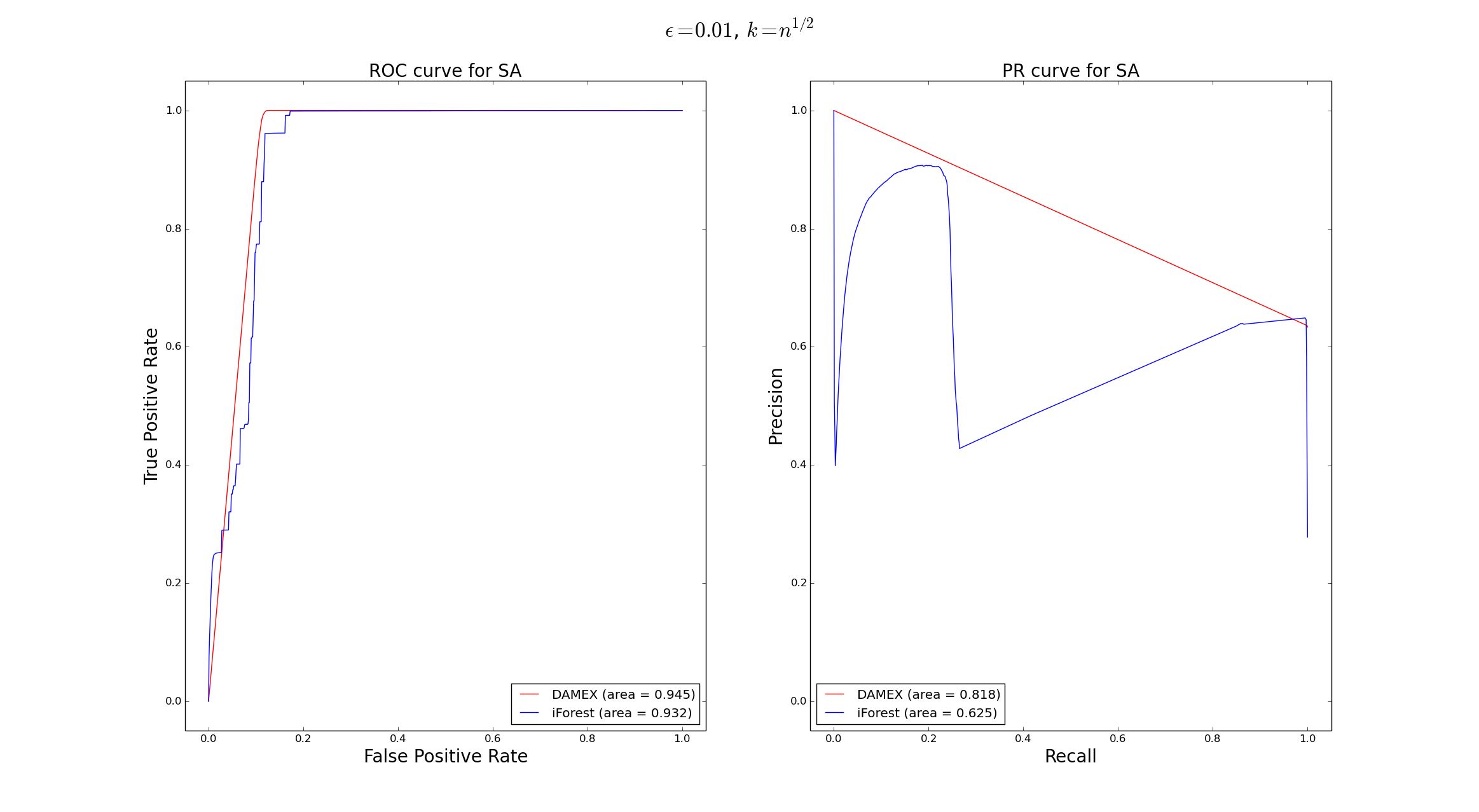
Figure 8: SA dataset, default parameters

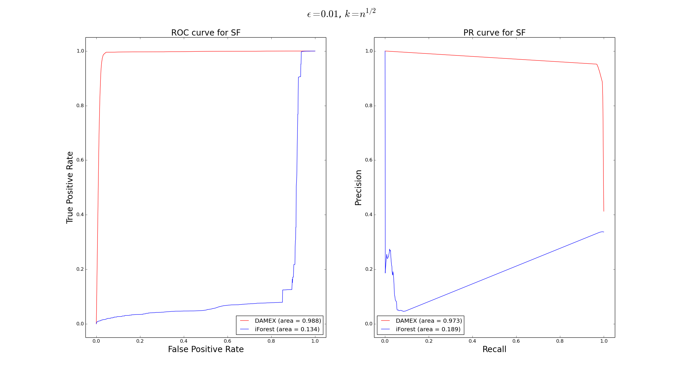
Figure 9: shuttle dataset, default parameters

Figure 10: http dataset, default parameters

References

References

• Aggarwal and Yu (2001) Aggarwal, C., Yu, P., 2001. Outlier detection for high dimensional data. In: ACM Sigmod Record. Vol. 30. pp. 37–46.
• Barnett and Lewis (1994) Barnett, V., Lewis, T., 1994. Outliers in statistical data. Vol. 3. Wiley New York.
• Beirlant et al. (2015) Beirlant, J., Escobar-Bach, M., Goegebeur, Y., Guillou, A., Feb 2015. Bias-corrected estimation of stable tail dependence function. https://hal.archives-ouvertes.fr/hal-01115538.
• Beirlant et al. (2004) Beirlant, J., Goegebeur, Y., Teugels, J., Segers, J., 2004. Statistics of Extremes: Theory and Applications. Wiley Series in Probability and Statistics. Wiley.
• Beirlant et al. (1996) Beirlant, J., Vynckier, P., Teugels, J. L., 1996. Tail index estimation, pareto quantile plots regression diagnostics. Journal of the American Statistical Association 91 (436), 1659–1667.
• Breunig et al. (1999) Breunig, M., Kriegel, H., Ng, R., Sander, J., 1999. Optics-of: Identifying local outliers. In: Principles of data mining and knowledge discovery. Springer, pp. 262–270.
• Chandola et al. (2009) Chandola, V., Banerjee, A., Kumar, V., 2009. Anomaly detection: A survey. ACM Computing Surveys (CSUR) 41 (3), 15.
• Clifton et al. (2008) Clifton, D., Tarassenko, L., McGrogan, N., King, D., King, S., Anuzis, P., 2008. Bayesian extreme value statistics for novelty detection in gas-turbine engines. In: Aerospace Conference, 2008 IEEE. pp. 1–11.
• Clifton et al. (2011) Clifton, D. A., Hugueny, S., Tarassenko, L., 2011. Novelty detection with multivariate extreme value statistics. Journal of signal processing systems 65 (3), 371–389.
• Coles (2001) Coles, S., 2001. An introduction to statistical modeling of extreme values. Springer Series in Statistics. Springer-Verlag, London.
• Coles and Tawn (1991) Coles, S., Tawn, J., 1991. Modeling extreme multivariate events. JR Statist. Soc. B 53, 377–392.
• Cooley et al. (2010) Cooley, D., Davis, R., Naveau, P., 2010. The pairwise beta distribution: A flexible parametric multivariate model for extremes. Journal of Multivariate Analysis 101 (9), 2103–2117.
• de Haan and Ferreira (2006) de Haan, L., Ferreira, A., 2006. Extreme value theory. Springer Series in Operations Research and Financial Engineering. Springer, an introduction.
• de Haan and Resnick (1977) de Haan, L., Resnick, S., 1977. Limit theory for multivariate sample extremes. Zeitschrift für Wahrscheinlichkeitstheorie und Verwandte Gebiete 40 (4), 317–337.
• Dekkers et al. (1989) Dekkers, A. L. M., Einmahl, J. H. J., de Haan, L., 12 1989. A moment estimator for the index of an extreme-value distribution. Ann. Statist. 17 (4), 1833–1855.
• Drees and Huang (1998) Drees, H., Huang, X., Jan. 1998. Best attainable rates of convergence for estimators of the stable tail dependence function. J. Multivar. Anal. 64 (1), 25–47.
• Einmahl et al. (2001) Einmahl, J. H., de Haan, L., Piterbarg, V. I., 2001. Nonparametric estimation of the spectral measure of an extreme value distribution. Annals of Statistics, 1401–1423.
• Einmahl et al. (2006) Einmahl, J. H. J., de Haan, L., Li, D., 08 2006. Weighted approximations of tail copula processes with application to testing the bivariate extreme value condition. Ann. Statist. 34 (4), 1987–2014.
• Einmahl et al. (2012) Einmahl, J. H. J., Krajina, A., Segers, J., 2012. An m-estimator for tail dependence in arbitrary dimensions. Ann. Statist. 40, 1764–1793.
• Einmahl et al. (2009) Einmahl, J. H. J., Li, J., Liu, R. Y., 2009. Thresholding events of extreme in simultaneous monitoring of multiple risks. Journal of the American Statistical Association 104 (487), 982–992.
• Einmahl and Segers (2009) Einmahl, J. H. J., Segers, J., 2009. Maximum empirical likelihood estimation of the spectral measure of an extreme-value distribution. The Annals of Statistics, 2953–2989.
• Embrechts et al. (2000) Embrechts, P., de Haan, L., Huang, X., 2000. Modelling multivariate extremes. Extremes and Integrated Risk Management (Ed. P. Embrechts) RISK Books (59-67).
• Eskin (2000) Eskin, E., 2000. Anomaly detection over noisy data using learned probability distributions. In: Proceedings of the Seventeenth International Conference on Machine Learning. pp. 255–262.
• Eskin et al. (2002) Eskin, E., Arnold, A., Prerau, M., Portnoy, L., Stolfo, S., 2002. A geometric framework for unsupervised anomaly detection. In: Applications of data mining in computer security. Springer, pp. 77–101.
• Finkenstadt and Rootzén (2003) Finkenstadt, B., Rootzén, H., 2003. Extreme values in finance, telecommunications, and the environment. CRC Press.
• Fougeres et al. (2015) Fougeres, A.-L., De Haan, L., Mercadier, C., 2015. Bias correction in multivariate extremes. The Annals of Statistics 43 (2), 903–934.
• Fougères et al. (2009) Fougères, A.-L., Nolan, J. P., Rootzén, H., 2009. Models for dependent extremes using stable mixtures. Scandinavian Journal of Statistics 36 (1), 42–59.
• Goix et al. (2015) Goix, N., Sabourin, A., Clémençon, S., 2015. Learning the dependence structure of rare events: a non-asymptotic study. In: Proceedings of the 28th Conference on Learning Theory.
• Goix et al. (2016) Goix, N., Sabourin, A., Clémençon, S., 2016. Sparse representation of multivariate extremes with applications to anomaly ranking. In: Proceedings of the 19th International Conference on Artificial Intelligence and Statistics. p. 287–295.
• Hill (1975) Hill, B. M., 09 1975. A simple general approach to inference about the tail of a distribution. Ann. Statist. 3 (5), 1163–1174.
• Hodge and Austin (2004) Hodge, V., Austin, J., 2004. A survey of outlier detection methodologies. Artificial Intelligence Review 22 (2), 85–126.
• Huang (1992) Huang, X., 1992. Statistics of bivariate extreme values.
• KDDCup (1999) KDDCup, 1999. The third international knowledge discovery and data mining tools competition dataset. KDD99-Cup http://kdd.ics.uci.edu/databases/kddcup99/kddcup99.html.
• Lee and Roberts (2008) Lee, H., Roberts, S., 2008. On-line novelty detection using the kalman filter and extreme value theory. In: Pattern Recognition, 2008. ICPR 2008. 19th International Conference on. pp. 1–4.
• Lichman (2013) Lichman, M., 2013. UCI machine learning repository.
URL http://archive.ics.uci.edu/ml
• Lippmann et al. (2000) Lippmann, R., Haines, J. W., Fried, D., Korba, J., Das, K., 2000. Analysis and results of the 1999 darpa off-line intrusion detection evaluation. In: Recent Advances in Intrusion Detection. Springer, pp. 162–182.
• Liu et al. (2008) Liu, F., Ting, K., Zhou, Z., 2008. Isolation forest. In: Data Mining, 2008. ICDM’08. Eighth IEEE International Conference on. pp. 413–422.
• Markou and Singh (2003) Markou, M., Singh, S., 2003. Novelty detection: a review—part 1: statistical approaches. Signal processing 83 (12), 2481–2497.
• Patcha and Park (2007) Patcha, A., Park, J., 2007. An overview of anomaly detection techniques: Existing solutions and latest technological trends. Computer Networks 51 (12), 3448–3470.
• Qi (1997) Qi, Y., 1997. Almost sure convergence of the stable tail empirical dependence function in multivariate extreme statistics. Acta Mathematicae Applicatae Sinica 13 (2), 167–175.
• Resnick (1987) Resnick, S., 1987. Extreme Values, Regular Variation, and Point Processes. Springer Series in Operations Research and Financial Engineering.
• Roberts (1999) Roberts, S., Jun 1999. Novelty detection using extreme value statistics. Vision, Image and Signal Processing, IEE Proceedings - 146 (3), 124–129.
• Roberts (2000) Roberts, S., 2000. Extreme value statistics for novelty detection in biomedical signal processing. In: Advances in Medical Signal and Information Processing, 2000. First International Conference on (IEE Conf. Publ. No. 476). pp. 166–172.
• Sabourin and Naveau (2012) Sabourin, A., Naveau, P., 2012. Bayesian dirichlet mixture model for multivariate extremes: A re-parametrization. Computational Statistics & Data Analysis.
• Schölkopf et al. (2001) Schölkopf, B., Platt, J. C., Shawe-Taylor, J., Smola, A. J., Williamson, R. C., 2001. Estimating the support of a high-dimensional distribution. Neural computation 13 (7), 1443–1471.
• Scott and Nowak (2006) Scott, C. D., Nowak, R. D., 2006. Learning minimum volume sets. The Journal of Machine Learning Research 7, 665–704.
• Segers (2012) Segers, J., 08 2012. Asymptotics of empirical copula processes under non-restrictive smoothness assumptions. Bernoulli 18 (3), 764–782.
• Shyu et al. (2003) Shyu, M., Chen, S., Sarinnapakorn, K., Chang, L., 2003. A novel anomaly detection scheme based on principal component classifier. Tech. rep., DTIC Document.
• Smith (2003) Smith, R., 2003. Statistics of extremes, with applications in environment, insurance and finance, chap 1. Statistical analysis of extreme values: with applications to insurance, finance, hydrology, and other fields. Birkhäuser, Basel.
• Smith (1987) Smith, R. L., 09 1987. Estimating tails of probability distributions. Ann. Statist. 15 (3), 1174–1207.
• Stephenson (2003) Stephenson, A., 2003. Simulating multivariate extreme value distributions of logistic type. Extremes 6 (1), 49–59.
• Stephenson (2009) Stephenson, A., 2009. High-dimensional parametric modelling of multivariate extreme events. Australian & New Zealand Journal of Statistics 51 (1), 77–88.
• Tavallaee et al. (2009) Tavallaee, M., Bagheri, E., Lu, W., Ghorbani, A., 2009. A detailed analysis of the kdd cup 99 data set. In: Proceedings of the Second IEEE Symposium on Computational Intelligence for Security and Defence Applications 2009.
• Tawn (1990) Tawn, J., 1990. Modelling multivariate extreme value distributions. Biometrika 77 (2), 245–253.
• Yamanishi et al. (2000) Yamanishi, K., Takeuchi, J., Williams, G., Milne, P., 2000. On-line unsupervised outlier detection using finite mixtures with discounting learning algorithms. In: Proceedings of the sixth ACM SIGKDD international conference on Knowledge discovery and data mining. pp. 320–324.