Representing Directed Trees as Straight Skeletons

Abstract

The straight skeleton of a polygon is the geometric graph obtained by tracing the vertices during a mitered offsetting process. It is known that the straight skeleton of a simple polygon is a tree, and one can naturally derive directions on the edges of the tree from the propagation of the shrinking process.

In this paper, we ask the reverse question: Given a tree with directed edges, can it be the straight skeleton of a polygon? And if so, can we find a suitable simple polygon? We answer these questions for all directed trees where the order of edges around each node is fixed.

1 Introduction

Many geometric structures on sets of points, line segments, or polygons, e.g. Delaunay triangulations, Voronoi diagrams, straight skeletons, and rectangle-of-influence graphs can be represented as graphs. The graph representation problem (for each of these geometric structures) asks which graphs can be represented in this way. That is, given a graph $G$, can we find a suitable input set $S$ of points, segments, or polygons such that the geometric structure induced by $S$ is equivalent to $G$?

Graph representation has been studied for numerous geometric structures in the past. To name just a few examples: Every planar graph is the intersection graph of line segments [5], every wheel is a rectangle-of-influence graph [10], and all 4-connected planar graphs are Delaunay triangulations [7]. See also [6] for many results on proximity drawability of graphs.

Of particular interest to our paper are two results. First, Liotta and Meijer [11] studied when a tree can be represented as the Voronoi diagram of a set of points, and showed that this is always possible (and the points are in convex position). Secondly, Aichholzer et al. [3] studied when a tree can be represented as the straight skeleton of a polygon, and showed that this is always possible (and the polygon is convex).

1.1 Background

The straight skeleton $\mathcal{S}(P)$ of a simple polygon $P$ is defined via a wavefront-propagation process: Each edge of $P$ emits a wavefront edge moving in a self-parallel manner at unit speed towards the interior of the polygon.

Initially, at time $t=0$, this wavefront is a single polygon that is identical to $P$. As the propagation process continues, however, the wavefront will change due to self-interaction: (i) In edge events, an edge of the wavefront shrinks to zero length and is removed from the wavefront. (ii) In split events, a vertex of the wavefront meets the interior of a previously non-incident wavefront edge. This split partitions the edge and the polygon into two parts that now propagate independently. (iii) If the input is not in general position, more complex interactions are possible. For example, entire portions of the wavefront collapse at once when parallel wavefronts that were emanated by parallel polygon edges meet, or new reflex wavefront vertices are created when multiple reflex vertices interact in a vertex-event. The propagation process ends once all components of the wavefront have collapsed. Therefore, the set of wavefront edges at any time $t$ form one or more polygons, which we call the wavefront and denote by $\mathcal{W}(t)$.

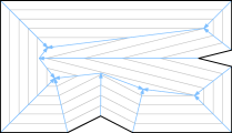
Figure 1: The straight skeleton $\mathcal{S}(P)$ of an input polygon $P$ (bold) is the union of the traces of wavefront vertices. Wavefront polygons at different times are shown in gray.

The straight skeleton $\mathcal{S}(P)$, introduced by Aichholzer et al. [2], is then defined as the geometric graph whose edges are the traces of the vertices of $\mathcal{W}(t)$ over time; see Figure 1. For simple polygons, $\mathcal{S}(P)$ always is a tree [2], with the leaves corresponding to vertices of $P$ and interior vertices having degree 3 or more. Several algorithms are known to construct the straight skeleton [1, 8, 9].

We can distinguish between convex and reflex vertices of $P$ or $\mathcal{W}(t)$. A vertex $v$ is reflex (convex) if the interior angle at $v$ is greater (less) than $\pi$. We call an arc of $\mathcal{S}(P)$ reflex (convex) if it was traced out by a reflex (convex) vertex of the wavefront. When discussing the wavefront propagation process, we will often interchangeably refer to wavefront vertices and straight skeleton arcs.

The roof model [2] represents a convenient means to study the wavefront over the entire propagation period. It embeds the wavefront in three-space, where the $z$-axis represents time: $\mathcal{T}(P):=\bigcup_{t\geq 0}(\mathcal{W}(t)\times\{t\})$. The inner edges and vertices of this polytope correspond to arcs and nodes of the straight skeleton $\mathcal{S}(P)$, and the $z$-coordinate of each element corresponds to the time it was traced out by the wavefront-propagation process. Reflex arcs correspond to valleys and convex arcs to ridges.

If we exclude polygons where parallel polygon edges cause entire wavefront segments to collapse at one time, resulting in horizontal roof edges, then arcs of $\mathcal{S}(P)$ will have been traced out by the wavefront during its propagation process, and we can assign a natural direction to these arcs: make them point into their trace direction. This assignment gives rise to the directed straight skeleton, $\mathcal{S}_{d}(P)$.

A directed tree $T$ is a directed graph whose underlying undirected graph is a tree, i.e., connected and acyclic. A labeled tree $T_{\ell}$ is a tree with assignments of labels to its arcs. For most of this paper, trees are ordered, i.e., for every node there is a fixed circular order in which the arcs appear around this node.

It is customary to refer to the edges and vertices of the straight skeleton as arcs and nodes, and to reserve edges and vertices for elements of input or wavefront polygons. We also use arcs and nodes to refer to elements of trees.

1.2 Our results

Our paper was inspired by the work in [3], which studies undirected trees. However, the structure of the straight skeleton imposes directions on the arcs, except in degenerate cases. Hence, the natural question to ask is:

Problem 1 (Directed straight-skeleton realizability)

Given a directed tree $T$, (i) is there a polygon $P$ such that $\mathcal{S}_{d}(P)$ shares the structure of $T$ (we denote this by $\mathcal{S}_{d}(P)\sim T$), and (ii) if yes, can we reconstruct such a polygon $P$ from $T$?

Having directions assigned to the arcs makes the straight-skeleton realizability problem significantly harder: For example, one easily sees that in a convex polygon the straight skeleton is a rooted tree (with exactly one sink), and so not all directed trees can be represented via convex polygons. Hence, the results from [3] do not transfer to directed trees.

The directed-straight-skeleton-realizability question can be asked for multiple meanings of “directed tree”: It could be a geometric tree (nodes are given with coordinates), an ordered tree (the clockwise order of arcs around each node is specified) or an unordered tree (we have the nodes and arcs but nothing else). For a geometric tree, the problem is trivial, since the locations of the leaves specify the vertices of the only polygon for which this could be the straight skeleton. (If leaves are not specified as points but only as “being on a ray”, then the geometric setting is non-trivial, but can be solved in polynomial time [4].)

In this paper, we consider the variant of the problem for ordered trees. In the case of polygons in general position, we give three obviously necessary conditions and show that these are also always sufficient. It turns out that the order of arcs around nodes is not important, so the algorithm also works for unordered directed trees. We then turn to polygons without restrictions on vertex-positions. In this case the directed straight skeletons can be significantly more complicated, and in particular, have arbitrary degrees. Testing whether a directed tree can be represented as straight skeleton requires deeper insight into the structure of straight skeletons, and we can exploit these to develop such a testing algorithm and, in case of a positive answer, find a suitable polygon.

2 Trees from Polygons in General Position

In a first step we restrict the problem to polygons in general position. By general position we mean that no four edges have supporting lines which are tangent to a common circle. In particular this means that during the wavefront propagation process only standard edge and split events are observed, resulting in straight skeletons where all interior nodes are of degree exactly three.

Investigating the structure of such directed straight skeletons enables us to establish a number of necessary conditions for a directed tree to be a directed straight skeleton of a polygon in general position.

Necessary conditions

Let $P$ be a polygon in general position and let $T$ be the directed tree such that $\mathcal{S}_{d}(P)\sim T$.

The leaves of $T$ correspond to the vertices of $P$. In the roof model, these vertices have zero $z$-coordinate, while all other nodes have positive $z$-coordinates since they will have been created by an event at some time $t>0$. Thus, any arc incident to a vertex $v$ of $P$ increases in elevation as it moves away from $v$. As such, all leaves of $T$ must have in-degree 0 and out-degree 1.

The interior nodes all have degree 3 and are classified by their in- and out-degrees as follows:

in-degree 3:

(peak nodes) A collapse of a wavefront component (of triangular shape) at the end of its propagation process is witnessed by a local maximum in the roof. These local maxima correspond to nodes with in-degree three.

in-degree 2:

(collapse nodes) Edge events in the propagation process, i.e., collapsed wavefront edges, result in a node with two incoming arcs and one outgoing arc.

in-degree 1:

(split nodes) Split events will cause a node that has only one incoming arc and two outgoing arcs.

in-degree 0:

Since the roof model will have no local minima except at the edges of $P$ [2], nodes with in-degree zero and out-degree three cannot exist.

Of these, the case of a split event requires some more attention since it imposes additional restrictions on the incoming arc. Recall that we can distinguish between reflex and convex vertices of $P$, and note that any vertex is either reflex or convex by the general position assumption. For a split event to occur, a reflex vertex of the wavefront must crash into a previously non-incident part of the wavefront.

In the absence of vertex events, which create skeleton-nodes of degree at least four and therefore do not happen when the polygon is in general position, no reflex vertex can ever be created by an event. Thus, any reflex vertex that is part of an event must have been emanating from a reflex vertex of the input polygon itself. Accordingly, the incoming arc in a split event node must have a leaf at its other end.

We summarize these conditions in the following lemma.

Lemma 1

Let $P$ be a simple polygon in general position and let $T$ be the directed tree such that $\mathcal{S}_{d}(P)\sim T$. Then in $T$

(G1)

the incident arc of each leaf is outgoing,

(G2)

every interior node has degree 3 and at most two outgoing arcs,

(G3)

if an interior node has out-degree two, then the incoming arc connects directly from a leaf.

Observations

Let $T$ be a directed tree that satisfies conditions (G1–G3). Classify the interior nodes as split nodes, collapse nodes and peaks as above. The goal is to show that any such tree can indeed be realized as a straight skeleton. For this, we split the tree into multiple subtrees in a particular way (also illustrated in the example in Figure 3). We have the following observations. Full proofs of the next four lemmas can be found in Appendix 0.A.

Lemma 2 ()

Let $T$ be a directed tree that satisfies conditions (G1–G3). If $T$ has no split nodes, then $T$ has exactly one peak.

Lemma 3 ()

Let $T$ be a tree that satisfies conditions (G1–G3). Create a forest $F$ as follows: At any split node $s$ of $T$, remove $s$, remove the leaf incident to the incoming arc of $s$, and replace the two outgoing arcs of $s$ by two new leaves that are connected to the other ends of these arcs. Then each component of $F$ satisfies conditions (G1–G3) and has exactly one peak.

Sufficient conditions

It remains to be shown that the necessary conditions (G1–G3) from 1 are also sufficient. We show this by constructing a simple polygon $P$ such that $\mathcal{S}_{d}(P)\sim T$, given a directed tree $T$ that satisfies (G1–G3). We start by showing this for trees that have no split nodes.

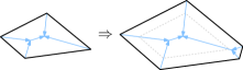
Figure 2: Creating the polygon for a tree with $k+1$ interior nodes from a polygon for a tree with one less.

Lemma 4 ()

For any directed tree $T$ that satisfies (G1–G3) and has no split nodes, there is a convex polygon $P$ such that $\mathcal{S}_{d}(P)\sim T$.

Proof

We show this by constructive induction. Any triangle is a polygon such that its straight skeleton shares the structure of the peak node of $T$.

To construct a polygon $P$ for a tree $T$ with $k$ interior nodes, we first construct a polygon $P^{\prime}$ for a tree $T^{\prime}$ with $k-1$ interior nodes. We obtain $T^{\prime}$ by replacing a node of $T$ and its two adjacent leaves with a single leaf $\ell$. (There always is such a node.) To obtain $P$, we compute an exterior offset of $P^{\prime}$ and replace the vertex that corresponds to $\ell$ with a sufficiently small edge such that it collapses before the wavefront of $P$ reaches $P^{\prime}$.

This polygon $P$ will then satisfy $\mathcal{S}_{d}(P)\sim T$. See Figure 2 for an illustration. ∎

Furthermore, it is possible to add a constraint on one interior angle of the polygon:

Lemma 5 ()

Let $T$ be a directed tree without split nodes and let $\ell$ be a leaf of $T$. Further, let $\alpha$ be an arbitrary angle with $0<\alpha<\pi$. Then there exists a convex polygon $P$ such that $\mathcal{S}_{d}(P)\sim T$ and such that the interior angle at the vertex that corresponds to $\ell$ is $\alpha$.

Now we are ready to consider trees with split nodes.

Lemma 6

Let $T$ be a directed tree that satisfies conditions (G1–G3). Then there exists a polygon $P$ such that $\mathcal{S}_{d}(P)\sim T$.

Proof

As in 3, we split $T$ at split nodes, also dropping the incoming reflex arc and its incident leaf. We obtain a forest $F=\{T_{1},T_{2},\ldots,T_{n}\}$ where each $T_{i}$ is a tree without split nodes.

This forest can in turn be considered an undirected tree, where each $T_{i}$ gives rise to a node and nodes are connected if and only if the corresponding trees originally had a split node in common. We pick an arbitrary root for $F$, say $T_{1}$, and construct a convex polygon $P_{1}$ such that $\mathcal{S}_{d}(P_{1})\sim T_{1}$.

This root $T_{1}$ is connected to one or more children in $F$ via split nodes. Let $T_{2}$ be such a child, and let $\ell_{1}\in T_{1}$ and $\ell_{2}\in T_{2}$ be the two leaves obtained when splitting at the split node common to $T_{1}$ and $T_{2}$. Let $v_{1}$ be the vertex in $P_{1}$ corresponding to $\ell_{1}$, and assume it has angle $\alpha_{1}<\pi$.

We construct a convex polygon $P_{2}$ such that $\mathcal{S}_{d}(P_{2})\sim T_{2}$ and the vertex $v_{2}$ corresponding to $\ell_{2}$ has angle $\alpha<\pi-\alpha_{1}$. This enables us to merge $P_{1}$ and $P_{2}$ in the following way: We place $P_{2}$ in the plane such that $v_{1}$ of $P_{1}$ and $v_{2}$ of $P_{2}$ occupy the same locus. We rotate $P_{2}$ such that the angle between a pair of edges of $P_{1}$ and $P_{2}$ is exactly $\pi$. Which pair of edges is chosen depends on where in the cyclic order the incident reflex leaf at the split node in $T$ lies. The layout of $P_{1}$ and $P_{2}$ then corresponds to the layout of the wavefront at the split-event time. If we now compute a small outer offset and designate this to be $P$, then the directed straight skeleton of $P$ has the same structure as the subtree of $T$ that is made up by $T_{1}$, $T_{2}$, the split node, and its incident leaf; see Figure 3.

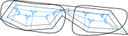
(a)

(b)

Figure 3: (a) Given a directed tree we split it into a forest $F$ of subtrees without split nodes. (b) Recursing on the structure of $F$, we can create convex polygons for each element (dotted) and then merge them into ever larger polygons.

We then repeat this process for another child of $T_{1}$ or $T_{2}$. Note that it may be necessary to scale the polygon that we add to a sufficiently small size so that it does not conflict with other parts of the polygon already constructed. This is always possible since for each vertex of a polygon there exists a disk that intersects the polygon only in the wedge defined by the vertex.

Once all elements of the forest have been processed, we have constructed a polygon $P$ whose straight skeleton has the same structure as $T$, i.e., $\mathcal{S}_{d}(P)\sim T$. ∎

Notice that conditions (G1–G3) do not depend on the order of arcs around nodes; we can construct a polygon for any such order. So in particular if $T$ is an unordered tree that satisfies (G1–G3), then we can pick an arbitrary order and the lemma holds. Hence, we get the following theorem:

Theorem 2.1

An (ordered or unordered) directed tree $T$ is the directed straight skeleton of a simple polygon $P$ in general position if and only if $T$ satisfies conditions (G1–G3).

3 Realizing trees with labeled arcs

Recall that an arc of the straight skeleton is called reflex (convex) if it was traced out by a reflex (convex) vertex of the wavefront. One can easily see that the construction in 6 creates a polygon where all arcs of the straight skeleton are convex, with the exception of arcs from leaves to split nodes.

For later constructions (for trees with higher degrees), it will be important that we test not only whether an ordered tree can be realized, but additionally we want to impose onto each arc whether it is reflex or convex in the straight skeleton. We study this question here first for trees with maximum degree 3.

So assume we have a directed tree $T$ that satisfies (G1–G3). Additionally we now label each arc of $T$ with either “reflex” or “convex”, and we ask whether there exists a polygon $P$ that realizes this labeled directed tree in the sense that $\mathcal{S}_{d}(P)\sim T$ and the type of skeleton-arc in $\mathcal{S}_{d}(P)$ matches the label of the arc in $T$. We denote this by $\mathcal{S}_{d}(P)\sim_{\ell}T$.

We observe that a peak node is created when a wavefront of three edges, a triangle, collapses. Therefore, all incident arcs at a peak node are convex.

For collapse nodes, we know that the outgoing arc is convex. (Recall that reflex arcs in a straight skeleton are only created in vertex events, which cannot exist when all interior nodes have degree three.) At least one of the incoming arcs needs to be convex, as two reflex wavefront vertices meeting in an event will result in a node of degree at least four.

We have already established that the incoming arc at a split node needs to be reflex. Furthermore, it is easy to see that the two outgoing arcs of a split node need to be convex.

We summarize the necessary conditions for a labeled directed tree to correspond to a straight skeleton in the following lemma:

Lemma 7

Let $P$ be a simple polygon in general position and let $T_{\ell}$ be the labeled directed tree such that $\mathcal{S}_{d}(P)\sim_{\ell}T_{\ell}$. Then

(L1)

for peak nodes, all incoming arcs are convex;

(L2)

for collapse nodes, at least one incoming arc and the outgoing arc are convex;

(L3)

for split nodes, the incoming arc is reflex and both outgoing arcs are convex.

We will now show that (L1–L3) are also sufficient:

Lemma 8

Any labeled directed tree $T_{\ell}$ that meets conditions (G1–G3) from 1 and (L1–L3) from 7 is realizable by a simple polygon $P$.

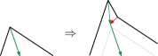
Figure 4: Extending a convex vertex of $P$ such that a leaf in its tree is replaced by a collapse node where one incoming arc is reflex and one is convex.

Proof

Since reflex arcs in $T_{\ell}$ only originate at leaves and terminate at collapse or split nodes (interior nodes never have outgoing reflex arcs, and peak nodes have no incoming reflex arcs), we can create a tree $T^{\prime}_{\ell}$ by replacing each collapse node that has an incoming reflex arc with a leaf and dropping the two incident incoming arcs and their leaves. This resulting tree $T^{\prime}_{\ell}$ will have no reflex arcs except for those leading from a leaf to split nodes by (L1), (L3), and (G3). Thus, we can create a polygon $P^{\prime}$ such that $\mathcal{S}_{d}(P^{\prime})\sim_{\ell}T^{\prime}_{\ell}$ by the process described in the proof of 6, respecting all labels.

We now obtain $P$ by offsetting $P^{\prime}$ slightly to the outside. Then, we modify $P$ at each vertex $v$ that corresponds to a leaf in $T^{\prime}_{\ell}$ that was the result of replacing a collapse node of $T_{\ell}$. Note that each such vertex $v$ is convex since the outgoing arc of a collapse node is convex by (L2). We insert a small edge in place of $v$, replacing it with $v_{1}$, the edge, and $v_{2}$. We choose the angles at $v_{1}$ and $v_{2}$ such that one of them is reflex and the other is convex, in order to match the labeling of $T_{\ell}$. Figure 4 illustrates this operation.

By making the new edge sufficiently small, we can ensure that these events happen before the wavefront becomes identical to $P^{\prime}$, and thus before all remaining events of the wavefront propagation. ∎

4 Arbitrary Node Degrees

Once we allow for straight skeletons where interior nodes can have degrees larger than three, a number of previous constraints no longer hold. Most importantly, during the wavefront propagation vertex events can happen, resulting in new reflex vertices in the wavefront after the event. Consequently, for instance, split nodes no longer need to be adjacent to leaves. Larger node degrees also result in more complex variants of split, collapse, and peak nodes. Note that we continue to restrict polygons from having parallel edges as those might cause skeleton arcs which have no direction (when they get created as a result of two wavefront edges crashing into each other) or straight skeleton arcs that are neither reflex nor convex (when two parallel wavefronts moving in the same direction become incident at an event).

In order to understand what combinations of reflex and convex incoming and outgoing arcs may exist at a node in a directed straight skeleton, we study the different shapes that a wavefront may have at an event at locus $p$ and time $t$. At a time $t-\delta$ immediately prior to the event, the wavefront will consist of a combination of reflex and convex vertices, tracing out reflex and convex arcs, all of which will meet at $p$ at time $t$. We choose $\delta$ sufficiently small such that no event will happen in the interval $[t-\delta,t)$.

Consider the wavefront around a locus $p$ at an event, and consider the wedges that have been already swept by the wavefront. With wedge we mean the area near $p$ swept over by a continuous portion of the wavefront polygon until time $t$.

If a single wedge covers the entire area around $p$, we call it a full wedge. The interior angles of other wedges might be less than $\pi$, greater than $\pi$, or exactly $\pi$ as illustrated in Figure 5. We call the first type of wedge reflex and the second type of wedge convex, after their corresponding wavefront vertices in the simple case. The third type of wedge we simply call $\pi$-wedge.

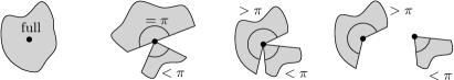
Figure 5: Wavefront wedges at event times are either full wedges or can be classified by their interior angle. The wedges (already-swept areas) are gray, the remaining white sectors are covered by the wavefront polygon(s).

A single wedge may have been traced out by just one wavefront edge if a wedge at an event has an interior angle of exactly $\pi$, but in all other cases it is the area covered by two or more wavefront edges and their incident wavefront vertices, which have traced out one or more incoming arcs at $p$. Note that all but the two outermost edges of this part of the wavefront collapse at time $t$.

We will establish arc-patterns to describe combinations of arcs at a node. Such a pattern is a string consisting of the types of arcs: $r$ for an incoming reflex arc, $c$ for an incoming convex arc, and $\hat{r}$ and $\hat{c}$ for their outgoing counterparts. We will use operators known from language theory, such as parentheses to group blocks, the asterisk $(^{*})$ to indicate the preceding character or group may occur zero or more times, the plus sign $(^{+})$ to indicate the preceding block may occur one or more times, and the question mark $(^{?})$ to indicate it may exist zero times or once. When defining patterns we give them variable names in capitals.

We now investigate which combination of arcs may trace out which types of wedges. For this purpose we first characterize single wedges and provide their describing arc-patterns. Then we examine all possible single wedge combinations and provide allowed arc-patterns for interior nodes.

In this section, we give only an overview of arc-patterns of single wedges and of arc-patterns for possible combinations of these wedges at interior nodes. For a detailed analysis please see Appendix 0.B.

As mentioned, single wedges can be reflex wedges, convex wedges, $\pi$-wedges, and so called full wedges, the latter being traced out by a wavefront that collapses completely around a locus $p$. The arc-pattern for a reflex wedge is $R:=r~{}(cr)^{*}$, i.e., one reflex vertex, followed by zero or more (convex, reflex) pairs of vertices and thus arcs. If a reflex wedge is created by a single reflex wavefront vertex (and its incident edges) then we call it trivial. Otherwise, we call it non-trivial, with $R_{+}=r~{}(cr)^{+}$ specifying the arc-pattern of a non-trivial reflex wedge.

The arc-pattern for a convex wedge is $C:=r^{?}~{}c~{}(r^{?}c)^{*}~{}r^{?}$. Like for reflex wedges we distinguish trivial (traced out by a single convex vertex) and non-trivial convex wedges, the latter (any pattern matching $C$ and having length at least two) being denoted by $C_{+}$.

The case of $\pi$-wedges is related to the case of reflex wedges. A $\pi$-wedge is either traced out by exactly one wavefront edge (no incoming arcs), or it has the same pattern as for a non-trivial reflex wedge. Hence, we have as arc-pattern $P:=\emptyset~{}|~{}R_{+}$. Note that since we have explicitly excluded parallel polygon edges for this problem setting, only trivial $\pi$-wedges can exist. Therefore, we will set $P:=\emptyset$ here.

Last, the arc-pattern of a full wedge is $F:=c~{}(r^{?}c)^{*}~{}c~{}(r^{?}c)^{*}~{}c~{}(r^{?}c)^{*}$.

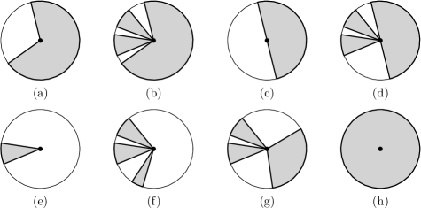
Figure 6: All wedge combinations possible at a node.

Analyzing possible combinations of single wedges at interior nodes we get seven different allowed arc-patterns (see Figure 6 (a-h)): $N_{a}:=C_{+}~{}\hat{c}$ , $N_{b}:=C~{}\hat{c}~{}(R~{}\hat{c})^{+}$ , $N_{d}:=P~{}\hat{c}~{}(R~{}\hat{c})^{+}$ , $N_{e}:=R_{+}~{}\hat{r}$ , $N_{f}:=(R~{}\hat{c})^{+}R~{}\hat{r}$ , $N_{g}:=(R~{}\hat{c})^{+}R~{}\hat{c}$ , and $N_{h}:=F$. (Note that the pattern from Figure 6 (c) will not result in an event without parallel polygon edges, which we have excluded.) A simple split node is matched via $N_{d}$, a simple collapse node is handled by $N_{a}$ (with $C_{+}$ being either $cc$, $rc$, or $cr$), and a simple peak node is matched by $N_{h}$.

Since these are all possible wavefront/wedge combinations, any interior node of the straight skeleton will have to match $N:=N_{a}|N_{b}|N_{d}|N_{e}|N_{f}|N_{g}|N_{h}$. We can state the following lemma:

Lemma 9

Let $P$ be a simple polygon and let $T_{\ell}$ be the labeled directed tree such that $\mathcal{S}_{d}(P)\sim_{\ell}T_{\ell}$. Then the cyclic order of arcs of any interior node of $T_{\ell}$ needs to match the pattern specification $N$ defined above.

After the necessity of the discussed conditions we now prove their sufficiency.

Lemma 10

Let $T_{\ell}$ be any labeled directed tree for which (i) the cyclic order of arcs of each interior node matches the pattern specification $N$ defined above and (ii) each leaf has out-degree one. Then $T_{\ell}$ is realizable by some simple polygon $P$, that is, $\mathcal{S}_{d}(P)\sim_{\ell}T_{\ell}$.

Proof

We will construct $P$ in a manner similar to the one described in 6. We start by identifying maximally connected components $C_{1},C_{2},\ldots,C_{n}$ of $T_{\ell}$ containing nodes with out-degree either zero or one. These components take the place of the subtrees of our forest from 6, and they are connected in $T_{\ell}$ via split-nodes, i.e., nodes with out-degree $\geq 2$.

We pick an arbitrary component $C_{1}$ and create a polygon $P_{1}$ such that $\mathcal{S}_{d}(P_{1})\sim_{\ell}C_{1}$ as follows. If there are no outgoing arcs from $C_{1}$, we start at its unique peak node. Otherwise, there is exactly one outgoing arc, and we begin at the node it is incident to. Constructing a polygon for this node is straightforward by applying the concepts learned from considering convex, reflex, and full wavefront wedges. We proceed by extending this initial polygon step by step like in 4, treating each reflex or convex vertex of the polygon as a wavefront wedge to be constructed, until we have a polygon for the entire component.

Next, we pick one of the split nodes connected to $C_{1}$. That split node, we call it $n$, will have one of the forms from Figure 6 that have at least two white sectors. The polygon we just created will cover one of these white sectors. (Depending on the type of arc connecting $C_{1}$ to $n$, the polygon will either have a reflex or convex vertex for this arc.) We continue by constructing polygons for all remaining white sectors in the same fashion we used for constructing $P_{1}$. Note that this process allows us to force at least one angle, and therefore we can construct polygons that fit into the white sectors for $n$.

Now we have the wavefront polygon as it should be when the event at $n$ happens. We compute a small exterior offset, joining all polygons into one larger polygon. The new reflex or convex vertices at this point are then further subdivided as required by the incoming arcs for $n$.

We repeat this process until we have covered all split nodes and thus all components and have thereby created a polygon whose structure matches $T_{\ell}$. ∎Please see Appendix 0.C for an example.

Combining 9 and 10, we obtain the following theorem:

Theorem 4.1

An ordered labeled directed tree $T_{\ell}$ is the directed straight skeleton of a simple polygon $P$ without parallel edges if and only if (i) the cyclic order of arcs of each interior node of $T_{\ell}$ matches the pattern specification $N$ defined above and (ii) each leaf has out-degree one.

Conclusion

In this work we developed a complete characterization of necessary and also sufficient conditions such that a given directed and labeled ordered tree can be represented as the straight skeleton of a simple polygon. This extends previous work on representing trees via related geometric structures [3, 11].

We leave the algorithmic question – how efficient suitability of a given input tree can be tested and, in case of an affirmative answer, a corresponding simple polygon can be computed – for future research. We conjecture that both is possible in time linear in the size of the given tree.

Appendix 0.A Proofs

0.A.1 Proof of 2 (See page 2)

See 2

Proof

Say $T$ has $k$ nodes and $k-1$ directed arcs. Since (G1–G3) hold, each node has out-degree exactly zero or one. There are $k-1$ arcs, so there are $k-1$ nodes with out-degree one. This leaves exactly one node with out-degree zero, the single peak node. ∎

0.A.2 Proof of 3 (See page 3)

See 3

Proof

Removing one $s$ gives three connected components. One of these is a leaf and removed. In the other two, we added a leaf with one outgoing arc, and for all other nodes in-degrees and out-degrees are unchanged. So (G1–G3) hold for all created components. Since out-degrees are unchanged, every component of the final forest $F$ has no split nodes, and hence a unique peak by the 2. ∎

0.A.3 Proof of 4 (See page 4)

See 4

This is a more verbose version of the proof:

Proof

We show this constructively by induction on the number of interior nodes of $T$. Recall that $T$ has a unique peak node.

In the base case, $T$ consists just of a peak node and three incident leaves. Choose an arbitrary triangle; the straight skeleton then has such a structure.

Now let us assume that for every tree $T$ with $k$ interior nodes we can find a convex polygon $P$ such that $\mathcal{S}_{d}(P)\sim T$.

Given $T^{\prime}$ with $k+1$ interior nodes we construct $P^{\prime}$ with $\mathcal{S}_{d}(P^{\prime})\sim T^{\prime}$ as follows. Find an interior node $n$ of $T^{\prime}$ that is incident to two leaves and obtain $T^{\prime\prime}$ from $T^{\prime}$ by dropping these two leaves, turning $n$ in $T^{\prime\prime}$ into a leaf. Since $T^{\prime\prime}$ has only $k$ interior nodes, we can find a convex polygon $P^{\prime\prime}$ such that $\mathcal{S}_{d}(P^{\prime\prime})\sim T^{\prime\prime}$.

To construct $P^{\prime}$, we compute a small exterior offset of $P^{\prime\prime}$ and replace the vertex corresponding to $n$ with a small edge. It should be sufficiently small that it will collapse before the wavefront propagating from $P^{\prime}$ reaches $P^{\prime\prime}$. This ensures that the event happens before any other in the wavefront propagation.

By this construction, the polygon $P^{\prime}$ will satisfy $\mathcal{S}_{d}(P^{\prime})\sim T^{\prime}$. See Figure 2 for an illustration. ∎

0.A.4 Proof of 5 (See page 5)

See 5

Proof

Let $p$ be the unique peak node in $T$, and let $p=v_{0},v_{1},\dots,v_{m-1},v_{m}=\ell$ be the nodes on the unique path from $p$ to $\ell$ in $T$. Pick a series of $m$ values $\alpha_{i}$ such that $0<\alpha_{1}<\alpha_{2}<\ldots<\alpha_{m-1}<\alpha_{m}=\alpha$.

When we create the triangle whose straight skeleton corresponds to the tree immediately around $p$, we choose it so that the angle at the polygon vertex corresponding to $v_{1}$ is $\alpha_{1}$. Throughout the expansion steps, we maintain that the angle at the vertex corresponding to $v_{i}$ (if it is a leaf of the current polygon) is $\alpha_{i}$.

When expanding the polygon at some leaf, we can choose the angle at one of the incident new vertices, as long as it is larger than the angle of the vertex replaced and less than $\pi$. See Figure 7 for an illustration.

Thus, if we expand at the vertex corresponding to $v_{i}$ (for some $i\geq 1$), it has angle $\alpha_{i}$, and we can pick the angle at the vertex corresponding to $v_{i+1}$ to be $\alpha_{i+1}$. At the end of the expansion the angle at the vertex that corresponds to $v_{m}=\ell$ is now $\alpha_{m}=\alpha$. ∎

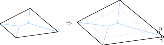
Figure 7: When extending a polygon, we can choose the angle at one of the two new vertices. The new angle can be an arbitrary value between the angle of the replaced vertex and $\pi$.

Appendix 0.B Details on allowed arc-patterns at interior nodes

We investigate which combination of arcs may trace out which types of wedges. For this purpose it is useful to look at the wavefront at a time $t-\delta$ immediately before the event, when all edges are still of proper length and not collapsed. We first consider single wedges and will afterwards discuss all possible combinations of them. Since all edges move at unit speed and reach $p$ exactly at time $t$, we know that just before the event their supporting lines must all be tangent to a common circle.

Reflex Wedges

First, let us look at reflex wedges (Figure 8). A reflex wedge can, of course, be created by a single reflex wavefront vertex and its incident edges. However, if it is created by more edges, then:

• The vertices incident to the two outermost edges ($e_{\ell}$ and $e_{r}$ in Figure 8) need to be reflex, because adding a convex vertex would introduce a wavefront edge that has already swept $p$ by time $t$.

• Since no two consecutive reflex vertices of the wavefront can become incident at an event (they always move away from one another), there needs to be a convex vertex between any two reflex vertices. This convex vertex will also reach $p$ at time $t$.

• Between two reflex vertices of a reflex wedge, no two consecutive convex vertices can exist. If they did, the wavefront edge between them at time $t-\delta$ would not be tangent to the circle and thus, would collapse prior to $t$, causing an event. However, we chose $\delta$ such that there is no event between $t-\delta$ and $t$.

• Any reflex vertex of the reflex wedge at time $t-\delta$ can in turn be replaced by a pair of reflex vertices with their convex vertex connector; cf. Figure 8 (3). This implies that an arbitrary number of reflex vertices can appear in one reflex wedge.

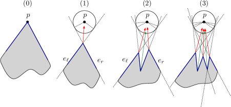
Figure 8: Wavefronts (bold, blue) of a reflex wedge at (0) and immediately before (1–3) an event. Area already swept over by the wavefront is shown in gray. All edges participating in the event have supporting lines that are tangent to the circle around the event location.

Summarizing, the pattern describing the arcs of a reflex wedge is $R:=r~{}(cr)^{*}$, i.e., one reflex vertex, followed by zero or more (convex, reflex) pairs of vertices and thus arcs.

We call a reflex wedge trivial if it was traced out by a single vertex and its two incident wavefront edges, and non-trivial otherwise. Let $R_{+}=r~{}(cr)^{+}$ be the pattern specification for a non-trivial reflex wedge.

Convex Wedges

A convex wedge in the simplest case is the result of a single convex vertex and its incident wavefront edges. More complex situations are possible: Many consecutive convex vertices may reach $p$ at the same time. Further, between any two convex vertices there may be one reflex vertex (see e.g. Figure 4 on how to replace a convex vertex with two vertices, one of them reflex). Even the outermost vertices in any collapsing chain need not be convex.

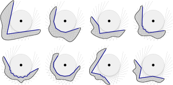
Figure 9: Wavefronts (bold, blue) of a convex wedge immediately before an event. Area already swept over by the wavefront is shown in gray. All edges participating in the event have supporting lines that are tangent to the circle around the event location.

Therefore, we can establish the pattern $C:=r^{?}~{}c~{}(r^{?}c)^{*}~{}r^{?}$ for a convex wedge.

Similar to before, we call a convex wedge trivial if it was traced out by a single vertex and its two incident wavefront edges and non-trivial otherwise. We use $C_{+}$ to denote any pattern matching $C$ and having length at least two, i.e., a non-trivial convex wedge.

$\pi$-wedges

A wedge with interior angle $\pi$ is related to the case of the reflex wedge. Either it is traced out by exactly one wavefront edge and there are no incoming arcs from this wedge to the event node, or it has the same pattern as for a reflex wedge. This is easy to see when again considering a time $t-\delta$ and the circle such that all participating wavefront edges lie in supporting lines tangential to the circle. Either it is just one edge, and it is tangential, or there are several and they need to start and end with reflex vertices to be tangent to the circle. Since in that case no wavefront edge actually touches the circle, we again cannot have more than one consecutive convex vertex.

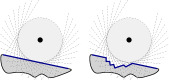
Figure 10: Wavefronts (bold, blue) of a $\pi$-wedge immediately before an event. Area already swept over by the wavefront is shown in gray. All edges participating in the event have supporting lines that are tangent to the circle around the event location.

We call a $\pi$-wedge trivial if it was traced out by a single wavefront edge and, hence, has no incoming arc, and non-trivial otherwise.

Thus, the pattern for a $\pi$-wedge is $P:=\emptyset~{}|~{}R_{+}$, that is, either it is empty or it is a non-trivial reflex-wedge pattern, i.e., with at least two reflex vertices.

Note that the outgoing arc of a non-trivial $\pi$-wedge is traced out by a vertex of the wavefront with interior angle exactly $\pi$. In such cases our problem statement that requires all arcs to be labeled either reflex or convex becomes invalid. We have therefore excluded polygons with parallel edges, and so for the purposes of this paper, only trivial $\pi$-wedges can exist. Therefore, we will set $P:=\emptyset$ here.

Full wedge

A full wedge is traced out by a wavefront that collapses completely around a locus $p$. In the simplest case this is a triangle. As in the case of the convex wedge we can replace any convex wavefront vertex with more convex wavefront vertices, and we can also put reflex vertices between any two convex vertices. The only constraint is that there need to be at least three convex vertices in total in order to close the wavefront polygon.

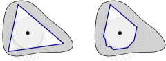
Figure 11: Wavefronts (bold, blue) of a full wedge immediately before an event. Area already swept over by the wavefront is shown in gray. All edges participating in the event have supporting lines that are tangent to the circle around the event location.

Therefore, the pattern for a full wedge is $F:=c~{}(r^{?}c)^{*}~{}c~{}(r^{?}c)^{*}~{}c~{}(r^{?}c)^{*}$.

Wedge combinations at events

Let us now consider which wedge combinations may be present at an event, and which outgoing wavefront vertices can be created in each case, cf. Figure 6.

So we have now defined patterns $R,R_{+},C,C_{+},P$, and $F$ for wedges that are reflex, convex, $\pi$-wedges, or full. Around each node, there may be many wedges, but at most one of them can be convex, $\pi$-wedge, or full.

one convex wedge:

If there is exactly one convex wedge, then it needs to be a non-trivial wedge. (Otherwise there would be no event.) The event will create a single convex outgoing wavefront vertex. The full pattern specification for this event therefore is $N_{a}:=C_{+}~{}\hat{c}$. See Figure 6 (a).

one convex wedge and one or more reflex wedges:

The $1+n$ wavefront wedges at the event leave a total of $1+n$ uncovered (white) sectors that the wavefront will soon sweep. For each of those, a single outgoing arc is created, and it must be convex since each unswept sector has an angle of less than $\pi$. $N_{b}:=C~{}\hat{c}~{}(R~{}\hat{c})^{+}$. See Figure 6 (b).

one $\pi$-wedge:

For this to be an event, the $\pi$-wedge needs to be non-trivial. The single vertex outgoing from this event will be connecting two wavefront edges sharing a common supporting line and will thus be neither reflex nor convex. We have excluded such cases in our problem statement. See Figure 6 (c).

one $\pi$-wedge and one or more reflex wedges:

This is an extended variant of the classic split event. The node’s pattern is $N_{d}:=P~{}\hat{c}~{}(R~{}\hat{c})^{+}$. See Figure 6 (d).

one reflex wedge:

The wedge has to be non-trivial, else there would be no event. So this is a vertex event, creating a new reflex vertex. $N_{e}:=R_{+}~{}\hat{r}$. See Figure 6 (e).

two or more reflex wedges all in the same half-plane:

Similar to the previous case, this must be a vertex event creating a new reflex vertex in the empty section whose interior angle is maximal (and thus larger than $\pi$). In all other sections a convex vertex is created. $N_{f}:=(R~{}\hat{c})^{+}~{}R~{}\hat{r}$. See Figure 6 (f).

two or more reflex wedges not all in the same half-plane:

Since there is no empty half-plane around the event, a new convex vertex will be created for each empty sector. $N_{g}:=(R~{}\hat{c})^{+}R~{}\hat{c}$. See Figure 6 (g).

full wedge:

If the complete disk around an event has already been swept by the wavefront, then a wavefront polygon is collapsing about the event location and we have a full wedge. $N_{h}:=F$. See Figure 6 (h).

Since these are all possible wavefront/wedge combinations, any interior node of the straight skeleton will have to match $N:=N_{a}|N_{b}|N_{d}|N_{e}|N_{f}|N_{g}|N_{h}$. Here, “matching” means matching cyclically, i.e., if a tree has a node where we find in cyclic order, a reflex outgoing, a reflex incoming, a convex incoming, and a reflex incoming, i.e., $\hat{r}~{}r~{}c~{}r$, then this would match $N_{e}=R_{+}~{}\hat{r}$ since we end up with two identical patterns by rotating one string cyclically.

Appendix 0.C Sample construction process (10)

Suppose we have a split node $n$ matching the pattern $r~{}c~{}r~{}\hat{c}~{}\hat{c}$, where each of those arcs has some more tree components on the side not at $n$; see Figure 12 (a).

We see that it is a split event, matching the one $\pi$-wedge and one or more reflex wedges case with $N_{d}:=P~{}\hat{c}~{}(R~{}\hat{c})^{+}$. Here, $P$ is the trivial $\pi$-wedge of $\emptyset$ and the only reflex wedge is $r~{}c~{}r$; see Figure 12 (b).

When we get to this split node, we already have created the polygon for one of the components $C_{1}$ or $C_{2}$. Assume we did $C_{1}$ already and produced $P_{1}$ (Figure 12 (c)). We next create a polygon $P_{2}$ for $C_{2}$, making sure that the angle at $n$ is sufficiently small to fit at $n$. In this example it needs to be less than $\pi-\alpha$ if $\alpha$ is the angle at $n$ for $P_{1}$.

(a)

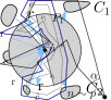
(b)

(c)

Figure 12: A split node of a tree (a) and its wedge representation (b). A possible polygon $P_{1}$ for $C_{1}$ (c).

Now that we have all the polygons present at the event node $n$, we place them on the plane such the vertices of $P_{1}$ and $P_{2}$ that correspond to the arc from $n$ become coincident in the same locus $p$. Since this is a split node with a trivial $\pi$-wedge we also need to rotate $P_{2}$ such that it forms an angle of exactly $\pi$ with $P_{1}$ on one side. Note that it may be necessary to scale $P_{2}$ such that it does not intersect anything already constructed.

Next, we compute a small offset of the merged polygons. The vertex $v$ illustrated in Figure 13 (a) currently stands for the entire reflex wedge. However, that wedge originates from three arcs, $r~{}c~{}r$, so we split that piece of the wavefront accordingly, see Figure 13 (b).

(a)

(b)

Figure 13: First we combine the two polygons for the individual components and compute an outer offset. Then we replace the vertex $v$ for the reflex wedge by a set of vertices tracing out all the arcs of the wedge.

References

- [1] Aichholzer, O., Aurenhammer, F.: Straight Skeletons for General Polygonal Figures in the Plane. In: Samoilenko, A. (ed.) Voronoi’s Impact on Modern Sciences II, vol. 21, pp. 7–21. Institute of Mathematics of the National Academy of Sciences of Ukraine, Kiev, Ukraine (1998)
- [2] Aichholzer, O., Aurenhammer, F., Alberts, D., Gärtner, B.: A Novel Type of Skeleton for Polygons. J. Univ. Comp. Sci 1(12), 752–761 (1995)
- [3] Aichholzer, O., Cheng, H., Devadoss, S.L., Hackl, T., Huber, S., Li, B., Risteski, A.: What makes a Tree a Straight Skeleton? In: Proc. 24th Canad. Conf. Comp. Geom (CCCG 2012). pp. 253–258. Charlottetown, PE, Canada (Aug 2012)
- [4] Biedl, T., Held, M., Huber, S.: Recognizing Straight Skeletons and Voronoi Diagrams and Reconstructing Their Input. In: Gavrilova, M., Vyatkina, K. (eds.) Proc. 10th Int. Sympos. Voronoi Diagrams in Sci. & Eng. (ISVD 2013). pp. 37–46. IEEE Computer Society, Saint Petersburg, Russia (Jul 2013)
- [5] Chalopin, J., Gonçalves, D.: Every Planar Graph is the Intersection Graph of Segments in the Plane (Extended Abstract). In: Proc. 41st Annu. ACM Sympos. Theory Comput. (STOC 2009). pp. 631–638. ACM, Bethesda, MD, USA (May 2009)
- [6] Di Battista, G., Lenhart, W., Liotta, G.: Proximity Drawability: A Survey. In: Tamassia, R., Tollis, I.G. (eds.) DIMACS International Workshop, Graph Drawing 94. LNCS, vol. 894, pp. 328–339. Springer, Princeton, NJ, USA (Oct 1995)
- [7] Dillencourt, M.B., Smith, W.D.: Graph-Theoretical Conditions for Inscribability and Delaunay Realizability. Discrete Math. 161(1-3), 63–77 (1996)
- [8] Eppstein, D., Erickson, J.: Raising Roofs, Crashing Cycles, and Playing Pool: Applications of a Data Structure for Finding Pairwise Interactions. Discrete & Comp. Geom. 22(4), 569–592 (1999)
- [9] Huber, S., Held, M.: A Fast Straight-Skeleton Algorithm Based On Generalized Motorcycle Graphs. Int. J. Comp. Geom. Appl. 22(5), 471–498 (Oct 2012)
- [10] Liotta, G., Lubiw, A., Meijer, H., Whitesides, S.: The Rectangle of Influence Drawability Problem. Comput. Geom. 10(1), 1–22 (1998)
- [11] Liotta, G., Meijer, H.: Voronoi Drawings of Trees. Comput. Geom. 24(3), 147–178 (2003)