Formation of accretion centers in simulations of colliding uniform density H₂ cores

Abstract

We test here the first stage of a route of modifications to be applied to the public GADGET2 code for dynamically identifying accretion centers during the collision process of two adjacent and identical gas cores. Each colliding core has a uniform density profile and rigid body rotation; its mass and size have been chosen to represent the observed core $L1544$; for the thermal and rotational energy ratios with respect to the potential energy, we assume the values $\alpha=0.3$ and $\beta=0.1$, respectively. These values favor the gravitational collapse of the core. We here study cases of both -head-on and off-center collisions, in which the pre-collision velocity increases the initial sound speed of the barotropic gas by up to several times. In a simulation the accretion centers are formed by the highest density particles, so we here report their location and properties in order to realize the collision effects on the collapsing and colliding cores. In one of the models we observe a roughly spherical distribution of accretion centers located at the front wave of the collision. In a forthcoming publication we will apply the full modified GADGET code to study the collision of turbulent cores.

Keywords: stars: formation– physical processes: gravitational collapse, hydrodynamics– methods:numerical.

1 Introduction

Stars form out of collapsing prestellar cores, located usually in larger clumps that could be isolated or part of a larger gas filament. Massive stars could also form as a result of the collapse of a relatively large core, [Zinnecker & Yorke (2007)]. Besides, the massive star formation scenario by means of gas collisions has gained observational support from recent space observation projects like ALMA, NANTEN, and the Spitzer telescope, all of which provide evidence of the occurrence of collisions among gas clouds and/or clumps, see section 1.1 of [Takahira et al.(2014)] and references there in.

Besides, [Testi et al.(2000)] have presented high-resolution interferometric and single-dish observations of molecular gas in the Serpens cluster-forming core. It appears that the Serpens core encompasses at least three substructures, the northwest and southeast sub-clusters and the near-IR cluster. Thus, the spatially distinct structures are also kinematically separated, while there is reasonable internal velocity coherence. Star formation is currently occurring simultaneously in the northwest and southeast sub-clusters, both of which contain roughly equal fractions of pre-stellar, proto-stellar, and IR sources. These facts point to the idea that Serpens was formed by means of a collision between two or three very similar gas clumps. [Graves et al. (2010)] and [Duarte-Cabral et al. (2010)] have recentely observed the Serpens molecular cloud by using HARP at the James Clerk Maxwell Telescope and reported evidence that Serperns consists of two colliding sub clouds.

Furthermore, [Furukawa et al. (2009)], [Torii et al.(2011)] and [Churchwell et al. (2006)], have reported about more recent observational evidence of cluster formation triggered by cloud-cloud collisions. They included the cases of RCW49, Westerlund2 and NGC3603 as examples. We then assume that collisions between smaller gas structures are also possible.

Turbulence makes a big change in the spatial distribution of the interstellar gas as turbulent clouds become filamentary and flocculent and their gas is locally compressed such that dense cores can form and eventually become gravitationally unstable to form stars, see for instance [Federrath & Klessen (2012)] and [Padoan et al.(2014)]. It is within highly turbulent molecular clouds where core collisions may occur because of the random nature of the gas velocity favors the formation of small over-densities across the cloud, which might be already collapsing or at least about to start collapsing.

Besides, [Motte et al. (1998)] have shown evidence that several parts of the Oph cloud have been compressed by an external pressure, such as a supernova explosion, an expanding HII region, or stellar wind shells. [Scoville et al. (1986)] have also presented observational evidence of gas compression at the interface of two colliding molecular gas regions. Thus, there is sufficient observational evidence to support the idea that gas collisions in all their possible size structures can occur. One can then ask what could be the influence of core collision on star formation.

Collision between relatively smaller clumps of gas and larger clouds have been studied numerically for more than three decades, for instance, [Hausman (1978)] and [Lattanzio et al. (1985)]; particularly, head-on collisions were considered by [Kimura & Tosa (1996)], [Klein & Woods (1998)] and [Marinho & Lepine (2000)]. Some of the earliest works were performed with only a few thousand particles and therefore suffered from a lack of resolution. However, in the recent past, simulations have been developed with much higher spatial resolution, for instance [Burkert & Alves (2009)] and [Anathpindika (2009a)]. The case of colliding gas structures starting from hydrodynamical equilibrium was considered by [Kitsionas & Whitworth (2007)] and [Anathpindika (2009b)]; [Anathpindika (2010)] has considered collisions between dissimilar gas structures.  [Gomez et al. (2007)] and  [Vazquez-Semanedi et al. (2007)] and other authors as well, have studied the generation of turbulence and star formation at the shock front of head-on collisions.

We here present numerical high resolution three dimensional hydrodynamical simulations of two rotating gas core collisions, including the self-gravity of the gas. We calculate all collision models with a modified GADGET2 code (which is describe in Section  3.3) in order to describe the formation of accretion centers in a collision system. We must clarify that accretion centers are conceptually simlar but not identical to the sink particles.

The sink particle technique, as implemented by [Bate et al. (1995)] and [Federrath et al. (2010)], has been very useful, as one of the most important issues in star formation numerical simulations is that of identifying peak density gas parcels and monitoring their evolution as closely as possible. In the case of the particle-based codes used to follow the gravitational collapse of cores, all the higher density particles are very closely packed, so that this set of particles is likely to be identified with a protostar. The sink particles play the role of proto-stars in the simulations and their physical properties are easily investigated in this scheme, which hopefully could be compared with observations. For instance, [Clark & Bonnell (2006)] have used the sink particle technique in their study of the mass function of cores by means of colliding clumpy flows.

We devote this paper to making new numerical simulations of the collision process of two rotating cores, taking advantage of both the new capabilities of modern computers and improved numerical techniques. We emphasize that a core very similar to the one which we take here, was originally suggested by [Whithworth & Ward-Thompson (2001)] as an empirical model to study the collapse of the well-observed core L1544. The physical properties of this core fit more or less the observed average properties of the cores reported by  [Tafalla et al.(2004)] and  [Jijina et al.(1999)]. [Tafalla et al.(2004)] have presented a multi-line and continuum study of L1544, and according to them this core presents evidence to be in an advanced state of evolution towards the formation of one or two low mass stars.

In this paper we take only the core size and mass as given by [Whithworth & Ward-Thompson (2001)], and we additionally consider the core to be in counterclockwise rigid body rotation around the $Z$ axis. We also include a density perturbation on the initial core model in order for the isolated collapsing core to develop a filament which eventually would fragment into a binary protostar system.

We here study collision effects on this collapsing core. The Rankine-Hugoniot jump condition applied to the case of two colliding cores, indicate that the density in the thin dissipative region where the collision takes place, must be increased by about four times the pre-collision density, so we expect an overdensity to be formed at the interface region of the colliding cores and also at the core’s central region where gravitational collapse is ongoing. The nature of the final distribution of proto-stars will depend on the collision parameters, mainly on the pre-collision velocity and the impact factor.

A word of warning is in order. In any star formation theory, it is very difficult to make numerical calculations with realistic initial conditions. Particularly difficult is the case of core collisions, where the parameter space is enormous and so we are here forced (like other authors, as already mentioned in the above paragraphs) to use simplified initial conditions. Despite this, we assess what are the effects of a collision on the collapsing and colliding cores, as well as where and when the accretion centers form, which are the most important issues to be investigated in this paper.

The outline of this paper is as follows. In Section 2 we describe the initial core, which will be involved in all the subsequent collision models. In Section 3 we give the details of the collision geometry and define the models to be studied. We shall also describe the modified GADGET2 code and the most important free parameters, which we fix by means of a calibration method presented in Section  3.3. In Section 4, we describe the most important features of the time evolution of our simulations by means of two-dimensional ($2D$) and three-dimensional ($3D$) plots. In Sections 5 and 6 we discuss the relevance of our results in view of those reported by previous papers and finally we make some concluding remarks.

2 The initial core

We consider a uniform density spherical core model with radius $R_{0}=8.0\,\times 10^{16}\,$ cm ($\,=0.026\;$ pc $\,=5350\;$AU) and mass $M_{0}=8\;M_{\odot}$. The average density of this core is $\rho_{0}=9.2\,\times 10^{-18}\;$ g   cm${}^{-3}\equiv 2.3\times 10^{6}\;$ part   cm^-3, from which an estimate of its free fall time is $t_{ff}=\sqrt{3\pi/(32G\rho_{0})}=6.9\times 10^{11}\,$ s $=21879\;$yrs.

The dynamical fate of a collapsing isolated core is usually characterized by the values of the thermal and rotational energy ratios with respect to the gravitational energy, denoted by $\alpha$ and $\beta$, respectively, see [Bodenheimer et al. (2000)] and [Sigalotti & Klapp (2001a)], [Sigalotti & Klapp (2001b)]. For this paper, all the simulations have been done with an initial core having the same initial values $\alpha$ and $\beta$

$$\begin{array}[]{l}\alpha\equiv\frac{E_{\rm therm}}{\left|E_{\rm grav}\right|}\approx 0.3\,,\vspace{0.25 cm}\\ \beta\equiv\frac{E_{\rm rot}}{\left|E_{\rm grav}\right|}\approx 0.1\,.\end{array}$$ (1)

As is well known, these values for $\alpha$ and $\beta$ favor the occurrence of core collapse. The speed of sound $c_{0}$ and the rotational angular velocity $\Omega_{0}$ have been calculated to satisfy the energy ratios given by Eq. 1; they have the following numerical values

$$\begin{array}[]{l}c_{0}\equiv 39956.8\,\mathrm{cm}\,\mathrm{s}^{-1}\,,\vspace{0.25 cm}\\ \Omega_{0}\equiv 8.09\;\times 10^{-13}\;\mathrm{rad}\,\mathrm{s}^{-1}\,.\end{array}$$ (2)

Then the initial velocity of the $i$th SPH particle is $\vec{v}_{i}=\vec{\Omega_{0}}\times\vec{r}_{i}=\Omega_{0}(-y_{i},x_{i},0)\,$.

Besides, we implement a well known spectrum of density perturbations on the initial particle distribution, so that at the end of the simulation they might result in the formation of binary systems. The evolution of a uniform density core like the model we consider here has been reproduced by many groups worldwide using different codes based both on grids and particles, see for instance [Bodenheimer et al. (2000)], [Sigalotti & Klapp (2001a)] and [Sigalotti & Klapp (2001b)] and the references there in. We have also successfully reproduced the uniform model results in [Arreaga et al. (2007), Arreaga et al. (2008)], from which we established the reliability of our calculations for the evolution of the core using the GAGDET2 code, as we followed the collapse process until peak densities of the order of $2.9\times 10^{-10}\,$ g  cm^-3.

Let us say something about the gas thermodynamics. As the observed star forming regions basically consist of molecular hydrogen cores at $10\,$ K with an average density of $1\times 10^{-20}\,$ g   cm ^-3, the ideal equation of state is a good approximation. However, once gravity has produced a substantial core contraction, the gas begins to heat. In order to take into account this increase in temperature, we use the barotropic equation of state proposed by [Boss et al. (2000)]. Thus, in this paper we carry out all our simulations using the barotropic equation of state

$$p=c_{0}^{2}\,\rho\left[1+\left(\frac{\rho}{\rho_{crit}}\right)^{\gamma-1}\,\right],$$ (3)

where for molecular hydrogen gas the ratio of specific heats $\gamma$ is given by $\gamma\,\equiv 5/3$, because we only take into account the translational degrees of freedom of the hydrogen molecule. The most important free parameter is then the critical density $\rho_{crit}$, which determines the change of thermodynamic regime. Here we consider only one value of $\rho_{crit}=5.0\times 10^{-14}\,$ g   cm^-3.

By comparing the results of our previous papers [Arreaga et al. (2007), Arreaga et al. (2008)] with those of [Whitehouse & Bate (2006)] for the collapse of an isolated and rigidly rotating core with a uniform density profile, we have concluded that the barotropic equation of state in general behaves quite well and that it captures all the essential thermodynamical phases of the collapse, see also [Arreaga & Klapp (2010)]. However, this does not mean that the same comparison would be always correct for more complex initial conditions or for collision models such as those we consider in this paper.

Despite these facts and that we know that it is indispensable to include all the detailed physics of the thermal transition in order to achieve the correct results, be it in a collision or not, we carry out the present simulations with the barotropic approximation, because we know that there are other computational and physical factors that could have a stronger influence on the outcome of a simulation.

The collision cores considered for this work have pre-collision velocities of up to several times the speed of sound, see Section 3 and Table 1. For these high velocities a particle agglomeration is formed in the interface between the cores and the artificial viscosity used for the calculations transforms kinetic into thermal energy, which increases the temperature of the gas. However, as we will show in Section 4.1, the cooling time $\tau_{cool}$ is both much shorter than the local sound crossing time, and the free fall time, hence the isothermal condition can be used for the interaction region.

3 Collision models and computational considerations

3.1 The pre-collision geometry

The simulations considered in this paper include both head-on and oblique collisions. For the head-on collisions, the initial position in cartesian coordinates of the center of mass (CM) of one colliding cores is at $(x,y,z)=\vec{X}_{CM_{1}}=(0,R_{0},R_{0})$ and the other at $\vec{X}_{CM_{2}}=(0,-R_{0},R_{0})$. Recall that $R_{0}$ is the initial core’s radius. The oblique collisions are characterized by the magnitude and sign of an impact parameter $b$, which depends on $R_{0}$. For the $b>0$ cases, the colliding cores are initially displaced along the $X$-axis. For the opposite case, when $b<0$, the cores are displaced again along the $X$-axis but in the opposite direction. In all cases the displacement is perpendicular to the symmetry axis of the collision (the $Y$-axis).

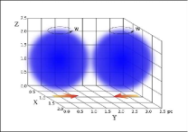
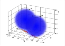
Figure 1: The initial geometry of the colliding cores for head-on collisions (left panel), and for oblique collisions with a positive impact parameter $b$ (right panel).

For instance, for model $M1$ we place the first core so that its center of mass in cartesian coordinates is $\vec{X}_{CM_{1}}=(R_{0}/4,R_{0},R_{0})$, while the center of mass of the second core is $\vec{X}_{CM_{2}}=(-R_{0}/4,-R_{0},R_{0})$. We consider this orientation as a positive impact parameter $b$, see Table 1 and Fig. 1. Analogously, for model $M3$, the center of mass of the cores is placed at the coordinates $\vec{X}_{CM_{1}}=(-b/2,R_{0},R_{0})$ and $\vec{X}_{CM_{2}}=(b/2,-R_{0},R_{0})$, which corresponds to a negative impact parameter.

For the collision models we consider four different impact parameter values $b=0,R_{0}/4,\pm\,R_{0}/2$, and pre-collision velocities in the range of 0.23 to 6.4 times the speed of sound. It should be noticed that this range of values is well motivated physically, as it follows from a statistical study of core collision in the context of interacting galaxies, see [Bekki et al. (2004)].

3.2 The pre-collision velocity

In this paper, we define the pre-collision velocity in the same way for both head-on and oblique collisions, as follows. The average velocity of the center of mass of the cores points along the $Y$-axis, and are $\vec{V}_{CM_{1}}=(0,-V_{ave},0)$ and $\vec{V}_{CM_{2}}=(0,V_{ave},0)$. We define the pre-collision speed $V_{app}$ (with respect to the center of mass of the colliding binary system) of the cores by means of $V_{app}=2\,V_{ave}$. Therefore, the pre-collision velocity $V_{app}$ of the colliding cores, also known as the relative or impact velocity of the cores, should be in the range $0.30-20$ Mach.

However, there must be a correlation between the pre-collision velocity of the colliding cores and their separation. As we assume here that the cores are initially in close contact, then we can not go to arbitrarily large values of the pre-collision velocities. Hence the values used here for $V_{app}$ have been chosen to represent an ample range, where the collision timescale can be compared with the free-fall time scale, as discussed in Section 5.

3.3 The Evolution Code

We carry out the time evolution of the initial distribution of particles with the fully parallel GAGDET2 code, which is described in detail by [Springel (2005)]. GADGET2 is based on the tree-PM method for computing the gravitational forces and on the standard SPH method for solving the Euler equations of hydrodynamics. GADGET2 incorporates the following standard features: (i) each particle $i$ has its own smoothing length $h_{i}$; (ii) the particles are also allowed to have an individual gravitational softening length $\epsilon_{i}$, whose value is adjusted such that for every time step, $\epsilon_{i}\,h_{i}$ is of order unity. GADGET2 fixes the value of $\epsilon_{i}$ for each time-step using the minimum value of the smoothing length of all particles, that is, if $h_{min}=min(h_{i})$ for $i=1,2...N$, then $\epsilon_{i}=h_{min}$.

The GADGET2 code has an implementation of a Monaghan-Balsara form for the artificial viscosity, see [Monaghan & Gingold (1983)] and [Balsara (1995)]. The strength of the viscosity is regulated by setting the parameter $\alpha_{\nu}=0.75$ and $\beta_{\nu}=\frac{3}{2}\,\times\alpha_{\nu}$, see Equation (14) in [Springel (2005)]. We fix the Courant factor to $0.1$. The number of smoothing neighbour particles is fixed to 40 and the allowed variation is fixed to 5 particles, so that the GADGET2 will adjust the kernel’s smoothing length such that the number of neighbours is always kept within the range 40 $\pm$ 5.

3.4 The detection of accretion centers

Let us now describe the modification implemented into the GADGET2 code to detect accretion centers. Any gas particle with density higher than $\rho_{s}$ is a candidate to be an accretion center. We localize all the candidate particles for a given time $t$. We then test the separation between candidate particles: if there is one candidate with no other candidate closer than $10\times r_{int}$, then this particle is identified as an accretion center at time $t$. We define $r_{int}$ as the neighbor radius for an accretion center, given by $r_{int}=1.5\times h_{min}$. In this way $r_{int}$ determines a set of particles which are within the sphere having this radius and whose center is the accretion center itself. All those particles will give their mass and momentum to the accretion center. We change the GADGET2 particle type for all those particles within the neighbor radius from being $0$ to $-1$, which is a particle type undefined in GADGET2 and therefore they will be not advanced in time anymore.

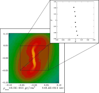
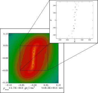
Figure 2: The last snapshots available for the collapse of the isolated core, for which we use the modified GADGET2 with density cutoff given by $\rho_{s}=1.0\times 10^{-12}\,$ g   cm^-3 (left panel), and $\rho_{s}=5.0\times 10^{-14}\;$g  cm^-3 (right panel).

We go on to determine an appropriate value of $\rho_{s}$ by using a uniform and rotating core model studied in previous collapse calculations. When we use a low value for $\rho_{s}$, for instance, $\rho_{s}=5.0\times 10^{-14}\,$g cm^-3, then too many accretion centers are formed even in an early collapse stage, see the right panel of Fig. 2. A better value for $\rho_{s}$ would be $\rho_{s}=1.0\times 10^{-12}\,$ g cm^-3, as the evolution of the test model both with and without the implemented code are quite similar.

The dependence of the number of accretion centers on the parameter $\rho_{s}$ can be considered as a depending way of discretize the densest gas region of interest. We emphasize that the radius $r_{int}$ and the $\rho_{s}$ are chosen here such that the formation of accretion centers does not affect the subsequent dynamics of the gas outside their influence region, otherwise it would be obviously a big problem in our simulations.

Furthermore, we mention here that [Klessen & Burkert (2000)] have used a clump finding algorithm, fully integrated into the SPH formalism, which makes no use of any parameters like ours $\rho_{s}$ and $r_{int}$.

However, other methods to detect sink particles like the one described by [Bate et al. (1995)] depends on three parameters: (i) a density threshold (which was chosen $10^{5}$ times higher than the average cloud density) to initially point to the gas candidate to be a sink particle; (ii) an accretion radius and (iii) an inner radius (which was defined to be 10-100 times smaller than the accretion radius).

[Bate et al. (1995)] applied the sink particle technique to study the collapse of the so called standard isotermal test case. Their objective was to extend the collapse calculation beyond the protostar formation by removing all those particles in the densest regions, which have very small time steps.

[Bate et al. (1995)] applied several collapsing and bounding tests on the gas particles inside the accretion radius before they are decided to be accreted or not by the sink particle. Besides, all those particles inside the inner radius are accreted by the sink particle regarless of the tests.

We must clarify that our parameter $r_{int}$ plays here the role of the inner accretion radius defined by [Bate et al. (1995)] and this is why we decide to skip all the tests as well. In a forthcoming revision of our code we will include an exterior radius $r_{ext}$ in order to detect and eventually eliminate all those particles located within an exterior influence region of an accretion center.

[Federrath et al. (2010)] implemented this sink idea in the mesh based code FLASH, which uses an adaptive mesh refiment (AMR) technique. They defined a sink cell and a sink volume by introducing two basic parameters: a density threshold and a radius. They went on to apply 6 tests on the sink cell to avoid the formation of spurious sinks. They found good agrement between this implementation and that reported by [Bate et al. (1995)] in the case of the core collapse. However, they emphasized that the use a sole density threshold parameter for deciding sink creation is insufficient when supersonic shocks are present.

Despite of all this, we carry out the time evolution of all the initial distribution of particles for the colliding models with a fixed value of $\rho_{s}=5.0\times 10^{-14}\,$ g cm^-3, because of the failure to evolve many of the particles of the colliding models until densities higher than $\rho_{s}$, otherwise the time step of the GADGET2 code becomes very small when not many particles are able to reach densities beyond $\rho_{s}$. As expected, all the collision models show a strong tendency to collapse like the isolated core, as can be seen in Fig. 3. The application of the limited technique described in this Section makes sense for us, as the main aim of this paper is only to detect the places where the densest region are formed when two rotating cores collide with a moderate pre-collision velocity.

3.5 Resolution

According to [Truelove et al. (1997)], the resolution requirement for avoiding the growth of numerical instabilities is expressed in terms of the Jeans wavelength $\lambda_{J}$, which is given by

$$\lambda_{J}=\sqrt{\frac{\pi\,c^{2}}{G\,\rho}}\;,$$ (4)

where $G$ is Newton’s universal gravitation constant, $c$ is the instantaneous sound speed and $\rho$ is the local density. To obtain a more useful form for a particle based code, the Jeans wavelength $\lambda_{J}$ is written in terms of the spherical Jeans mass $M_{J}$, which is defined by

$$M_{J}\equiv\frac{4}{3}\pi\;\rho\left(\frac{\lambda_{J}}{2}\right)^{3}=\frac{\pi^{\frac{5}{2}}}{6}\frac{c^{3}}{\sqrt{G^{3}\,\rho}}\;.$$ (5)

Nowadays it is well known that the Jeans requirement $l<\lambda_{J}/4$ (where $l$ is a characteristic length scale of the grid for a mesh based code) is a necessary condition to avoid the occurrence of artificial fragmentation. For particle based codes, [Bate & Burkert (1997)] showed that there is also a mass limit resolution criterion which needs to be fulfilled besides that of [Truelove et al. (1997)]. They showed that an SPH code produces correct results involving self-gravity as long as the minimum resolvable mass is always less than the Jeans mass $M_{J}$.

Now, if we approximate the instantaneous sound speed by $c=\sqrt{p/\rho}$, then according to Eq. 3, we have that

$$M_{J}=\frac{\pi^{\frac{5}{2}}}{6}\;\frac{c_{0}^{3}}{\sqrt{G^{3}\,\rho}}\;\left[1+\gamma\,\left(\frac{\rho}{\rho_{crit}}\right)^{\gamma-1}\right]^{\frac{3}{2}}\;.$$ (6)

Following [Bate & Burkert (1997)], the smallest mass that an SPH calculation can resolve is $m_{r}\approx M_{J}/(2N_{neigh})$, where $N_{neigh}$ is the number of neighbor particles included in the SPH kernel. For our collision models to comply with the Jeans requirement, the particle mass $m_{p}$ must be such that $m_{p}/m_{r}<1$.

In this work, we set $N=1,000,000\;$ SPH particles for representing the initial core configuration in each model. By means of a rectangular mesh we make the partition of the simulation volume in small elements each with a volume $\Delta x\,\Delta y\,\Delta z$; at the center of each volume we place a particle -the $i-th$, say- with a mass determined by its location according to the density profile being considered, that is: $m_{i}=\rho(x_{i},y_{i},z_{i})\,\Delta x\,\Delta y\,\Delta z$ with $i=1,...,N$. Next, we displace each particle from its location a distance of the order $\Delta x/4.0$ in a random spatial direction.

For verifying that the Jeans stability condition is satisfied we will use the collision model $HO-3$, which is the one that reached the highest maximum density of all models, see Table 1. For this model we follow its collapse until a peak density of $\rho_{max}=2.8\times 10^{-10}\;$g cm^-3. The particle mass is $m_{p}\equiv 2\,M_{0}/N_{p}=8\times 10^{-6}M_{\odot}$, where $M_{t}=16M_{\odot}$ is the total mass contained in the simulation box and $N_{p}$ is the total number of particles, which are $2$ million for all the models in this paper.

The minimum Jeans mass for model $HO-3$ is given by $\left(M_{J}\right)_{HO-3}\approx 8.6\times 10^{-4}\;M_{\odot}$, from which we obtain $m_{r}=1.0\times 10^{-5}\,M_{\odot}$. Thus, for model $HO-3$ we obtain the ratio $m_{p}/m_{r}=0.74$, and the Jeans resolution requirement is satisfied very easily.

For the rest of the collision models, the minimum Jeans mass is expected to be greater than for model $HO-3$ because their maximum density is less than for model $HO-3$. It is then clear that for all models the Jeans length criterion is satisfied as well.

3.6 Collision models

We summarize the collision models considered in this paper in Table 1, whose entries are as follows. Column one shows the label chosen to identify the model. Column two indicates the impact parameter $b$ of the collision models in terms of $R_{0}$; note the appearance of a sign before the magnitude of $b$, which is related to the orientation of the colliding cores along the $X$-axis, see Section 3.1. Column three indicates the pre-collision velocity of the colliding cores, expressed in terms of the initial speed of sound in the core, whose numerical value is given in Eq. 2. In the fourth column we show the number $N_{acc}$ of accretion centers found for each system, both for the case of an isolated core and for the colliding models. In the fifth column we show the average number of SPH particles $Np_{acc}$ per accretion center formed in each model while in the sixth column we show average mass of the accretion center $M_{av}/M_{sun}$. As a way of comparing our simulations with other simulations, in the seventh column we show the peak density $\rho_{max}$ reached in each run.

4 Results

In order to show the results of our simulations, we present iso-density plots for a slice of matter parallel to the $X-Y$ plane. The procedure is as follows. We first locate the SPH particle with the maximum density in the entire volume space of a simulation. The $z$-coordinate of that particle, say $z_{max}$, determines the height of the thin slice of material. The width of the slice is determined so that about $10,000\,$SPH particles enter into the slice, which is centered around the $z_{max}$ coordinate.

Once the SPH particles defining the slice have been selected, we set a color scale related to the iso-density curves: yellow indicates areas with higher densities, blue indicates those with lower densities, and green and orange indicate intermediate density regions. It should be noted that there is no relation between the density colors associated with different panels even in the same plot. At the bottom of each iso-density panel, we include two numerical values to illustrate the different stages of the evolution process: the left value is the peak density $\rho(t)$ at time $t$; and the right one is the actual time $t$ in seconds.

4.1 The general picture of a core collision

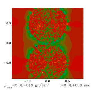
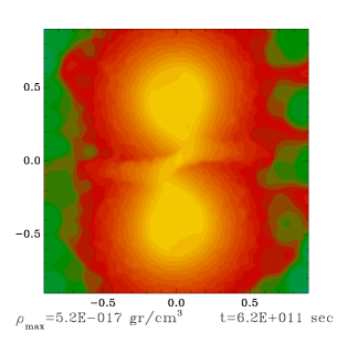
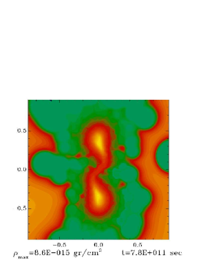
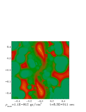
Figure 4: Iso-density plot illustrating the gravitational collapse process for model $HO1$ computed with the normal GADGET2 code.

Let us now briefly describe the general picture of a collision system by using the evolution of model $HO-1$ as an example, calculated using the normal GADGET2 code just for comparison. In the first top left panel of Fig. 4, one can see that two identical cores are just placed one against the other at $t=0$. Each core shares those particles which are closer to the edge of the neighboring core.

As each core in the colliding system is collapsing separately as well, we see in the right bottom panel of Fig. 4 the formation of a filament in each central core region. Such filaments are indeed connected by a gas bridge that is formed in the interface region of the cores.

The interface particles are compressed and a front perturbation is formed that propagates into the two cores. The artificial viscosity then transforms kinetic energy into heat. We expect that the barotropic equation of state proposed by [Boss et al. (2000)] and described in Eq. 3 mimics the radiative cooling needed as this heat must be radiated away in a very short timescale, so that we can assume that the cores and the interface region between the cores remain isothermal. The perturbation wave that propagates into the cores can disturb the filaments in the central region.

During the collision process a slab of material is formed along the collision front. The cores then expand but eventually collapse again. The compressed slab formed is susceptible of having various instabilities, which have been studied by [Vishniac (1983)] for the linear regime, and by [Vishniac (1994)] for the non-linear case. For the present work, the relevant instabilities are the shearing and the gravitational. The shearing instability dominates at low density while the gravitational one takes over for densities above the critical density

$$\rho_{shear}\,\sim 7.86132\,\times 10^{-22}\left(\frac{\eta}{pc}\right)\left(\frac{\lambda_{NTSI}}{pc}\right)\left(\frac{T}{K}\right)\,\mathrm{g}\,\mathrm{cm}^{-3},$$ (7)

where $\eta$ is the amplitude of the perturbation, $\lambda_{NTSI}$ the length of the unstable mode, and $T$ the temperature, see [Heitsch et al. (2008)].

Of the shearing instabilities, the main ones are the non-linear thin shell instability (NTSI), and the Kelvin-Helmholtz (KH) instability. The NTSI instability is expected to occur in the shocked slab just after the core collision, and the non-linear bending and breathing modes could also be present. From our numerical results we estimate that the parameters in Eq. 7 are $\lambda_{NTSI}\,\sim\,0.1\,$ pc, $\eta\,\sim 2\,\lambda_{NTSI}$ and $T\,\sim\,10\,$ K, and so the $NTSI$ and $KH$ instability are suppressed when the density goes above $\rho_{crit}\,\sim 1.57\,\times 10^{-18}\,$g   cm^-3.

In the next sections we shall describe the results obtained with the modified GADGET2 code for the time evolution of all models. The aim is to locate accretion centers and to determine their properties along the filaments and at the interfacial region as well.

4.2 Head-on collisions

In Fig. 5 we show the last snapshot available for each collision model, or in other words, for the sake of brevity, we omit presenting the earlier states of the evolution, like the first three panels shown in Fig. 4.

With $V_{app}$ slightly less than $c_{0}$, which corresponds to model $HO-3$, the initial cores are slightly disturbed, as the central filament shows a little stretching.

Most of the gas in the filament remains there as the collapse of each core progresses further. As we see in Fig. 2, many accretion centers are expected to be formed along these filaments, giving place to the formation of a peculiar chain of protostars when the gas cools further.

In the top panel of Fig. 6 we show the velocity field of the particles located near the filament. It can be seen that these particles flow into the filament. In Fig. 8, we show a $3D$ visualization of the same filament of model $HO2$ seen from a different angle; in this view, it is possible to observe that a very small over-density is formed at each filament’s end, at the colliding interface between the two collapsing cores. The origin of these new over-densities is the density perturbation caused by the core collision.

With a higher pre-collision velocity, self-gravity will have less time to act on the core and many more particles from the cores would flow very quickly to the cores’ interface, up to the point that the two initial cores can no longer be distinguished, as can be seen in models $HO-6$ and $HO-7$. For these models, the net effect of the collision is then to replace the two initial colliding cores by only one core, which rapidly forms a long central filament-like structure. In the bottom panel of Fig. 6, we observe again the formation of a strong filament in the interface of the cores that expands rapidly as a strong flow of particles go by the ends along the $X$-axis. However, the expansion eventually stops and the filament bounces to re-initiate the expansion in the transversal direction, along the $Y$-axis. This behavior has previously been observed by [Anathpindika (2009a)].

Thus, one effect of having a higher pre-collision velocity is that the density perturbation is stronger as can be seen in the last panel of Fig. 5. If $V_{app}$ is high enough, we see that the net effect of the collision is to replace the two initial colliding cores by one core which may not be collapsing anymore.

4.3 Oblique collisions

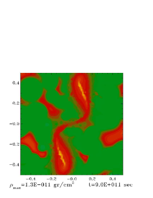
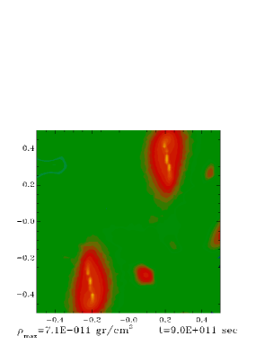
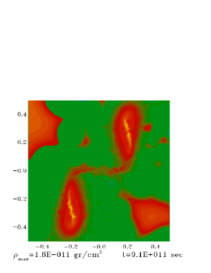
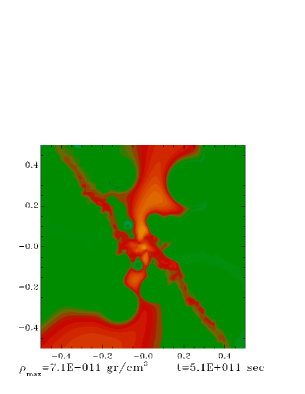
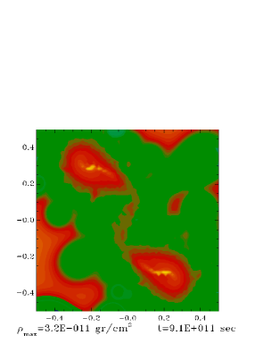
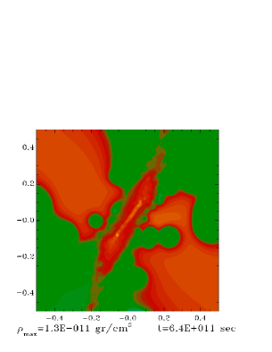
Figure 7: Iso-density plots for the last available snapshot for the oblique collision models $M1$ (top left panel), $M2$ (top middle panel), $M21$ (top right panel), $M22$ (bottom left panel), $M3$ (bottom middle panel), and $M4$ (bottom right panel).

The outcome for the oblique models is illustrated in Fig. 7, where we show only the last available snapshot of each model. As expected, the results for model $M1$, with a low pre-collision velocity and with small impact parameter value, are quite similar to those obtained for the head-on collision models $HO-1$, $HO-2$ and $HO-3$. Hence, it is unnecessary to calculate more models with increasing $V_{app}$ with a small impact parameter, because we would expect to see similar results to those obtained for the head-on collision models.

We then go on to models $M2$, $M21$ and $M22$, where the impact parameter has been increased to $b=R_{0}/2$, again with the positive orientation. The pre-collision speed is low for the two former models and higher for the later model. Similar results are obtained for models $M3$ and $M4$, where we change the orientation of the impact parameter.

The net effect of a high $V_{app}$ on the colliding system is evident in models $M22$ and $M4$, as the two cores get dispersed to give place to a long filament. It must be emphasized that the orientation and the width of these filaments are different from the ones obtained for the high $V_{app}$ head-on collision models.

4.4 Formation and location of the accretion centers

In order to show the results of this section, we present $3D$ plots of all the particles located in a central cube (with half the length of the side of the original simulation box) and whose density is greater than $1.2\times 10^{-17}\,$ g  cm^-3, see Fig. 8. As in Section 4, we again set a color scale related to density: red and orange indicate particles with higher densities, blue those with lower densities, and and yellow the intermediate density particles, see the caption of Fig. 8. It should be noted that there is no relation between the density colors associated with different panels even in the same plot. We rotate each panel as needed for the purpose of better appreciating the location of the accretion centers.

As expected, the pre-collision velocity $V_{app}$ also has a strong influence on the number and location of accretion centers, as it seems that the greater the $V_{app}$ the lower the $N_{acc}$. As can be seen in Fig. 8, if $V_{app}$ is too low, the initial binary core system survives even to an advanced stage of the evolution, and the accretion centers are mainly localized in the core’s central filament. But if $V_{app}$ is too high, then the initial binary core system is destroyed by the strong flow of particles, giving less chance for accretion center to form. For models $HO-3$ and $HO-6$, the accretion centers are indeed located mainly in the cores’ interface, as can be seen in the close-up shown in Fig. 8.

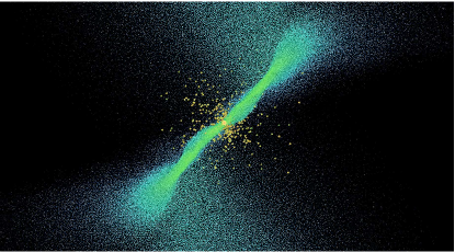
Figure 9: Zoom in of the left panel of the second line in Fig. 8, where the accretion centers are shown for model $HO3$.

It is therefore remarkable to realize that models $HO-2$ and $HO-3$ have accretion centers forming outside the core’s central filament, as can be seen in Fig. 8. As we can see, there must be a small range of velocities $V_{app}$ which favors the formation of accretion centers in the gas bridge connecting the two cores, see Fig. 9.

From Table 1, we first notice that the oblique collision models have a larger number of accretion centers than the head-on models. It seems that more accretion centers are created if self-gravity has more time available to act on the collapsing cores.

5 Discussion

For this paper we carried out a fully $3D$ set of numerical hydrodynamical simulations within the framework of the SPH technique, aimed at following the formation of accretion centers in a collision process of two small rotating cores with uniform density.

The initial conditions for the isolated core are such that it will collapse because its initial $(\alpha+\beta)_{core}<0.5$. However, when we consider the translational kinetic energy that comes from the pre-collision velocity $V_{app}$ of the cores, the collision system is expected to be slightly unbound, that is, $(\alpha+\beta)_{collision}>0.5$ for all models. As a result of the collision process, a large fraction of the translational kinetic energy will be transformed into heat, which will be radiated away because the cores and the perturbation front that forms in the interphase between the cores are isothermal. This must somehow produce a reduction of the global value of $(\alpha+\beta)$ for our collision models, as we observe that most of them are on the verge of gravitational collapse, see Fig. 3.

We have seen that the result of a collision simulation depends mainly on two physical factors that compete to exert influence on the collision process. These factors are the self-gravity and the flow of the particles from the colliding interface. The occurrence and extension of these factors are regulated by the value of the pre-collision velocity $V_{app}$ of the collision system.

With a very slow pre-collision velocity, self-gravity dominates the evolution of both cores. In such cases, the main effect of self-gravity on the system is to reduce the core size. The collision system quickly reaches a configuration in an advanced state of gravitational collapse, consisting of the remains of each collapsed core linked by a bridge of matter. We note that the accretion centers in the simulations are always located in the gas remnants of the cores. In most collision cases, we expect these accretion centers to separate from the filamentary structure, so that each fragment is expected to evolve towards virial equilibrium.

On the other hand, when a collision takes place with a significant pre-collision velocity, self-gravity plays a minor role and the fate of the system is entirely determined by the strong flow of particles in the interface of the cores. In these cases, the main effect on the system is to replace the two initial collapsing cores by a single core that rapidly gets perturbed to give place to an elongated and irregular filamentary structure formed in the interaction region. This filamentary structure increases its size very rapidly as it is continuously fed by in-falling material coming from the original cores. In these cases, we observe that accretion centers are formed in the central region of this filament structure.

However, in view of the limited nature of our simulations, the future of this filamentary structure is as yet unclear; but it is likely that most of the gas already in the filament will stay in this filamentary structure as the collapse progresses further. Although accretion centers may be formed near the bridge edges, as we see in the case of model $HO-2$, these accretion centers will be very thin and small, so it could be the case that their diameter will be greater in general than the Jeans length. This is another reason why the bridge would not be an appropriate site for proto-stellar formation until it cools further.

The results obtained for model $HO-3$ have been emphasized by zooming in on the filament’s central region, as shown in Fig. 9. We here see the formation of a well defined central accretion center, which is surrounded by many smaller accretion centers. The properties of this clustered distribution of protostars will be discussed elsewhere.

Now, according to Table 2, the maximum evolution time reached by the models is in the range $0.6<t_{evol}/t_{ff}<1.3$, where the free fall time $t_{ff}$ was defined in the first paragraph of Section 2. Except for models $HO-6$ and $HO-7$, all the other models have reached a $t_{evol}$ greater than $t_{ff}$. It should be noticed that most models have therefore evolved in time up to an advanced stage of collapse. Unfortunately, it is not possible to compute most of the models any further, as the time step becomes very small.

The relevant time scale for the collision is given approximately by $t_{col}\approx R_{0}/V_{app}$. For the models of this paper, this collision time is in the range $0.5<t_{col}/t_{ff}<12$. For model $HO-6$ these time scales are of the same order, $t_{col}/t_{ff}\sim 1$. By looking at Fig. 5, we see that the pre-collision velocity of model $HO-6$ is the maximum collision velocity that allows an initial binary colliding core system to remain as a binary system capable of undergoing further gravitational collapse and eventually of producing multiple protostars. It is in this sense that our results have to be compared with those of [Whithworth & Pongracic (1991)], who found that it is more likely that a colliding system will in general result in disruption and dispersal of the core involved, with no chance of forming protostars.

6 Concluding Remarks

In this paper we have been able to demostrate some of the essential features of the two core collision processes. In a first approximation, we have investigated the number and location of the accretion centers formed in this collision scheme.

The modified GADGET2 code tested here and described in Section 3.3 is a first step towards the full sink-particle technique implementation already in use worldwide. Our code is still incomplete as we have not yet included all the particle tests suggested by [Bate et al. (1995)] and [Federrath et al. (2010)]. However, as we have applied the same code to all the models, a comparison is possible. The main results of this comparison are shown in Table 1 and in Fig. 8.

It must be taken into account that (i) we have used a low density threshold $\rho_{s}$ for a particle to become an accretion center and (ii) there is no restriction on the minimum number of particles that must be captured for a particle to become an accretion center: so we have seen that there are a large number of accretion centers having just very few captured particles. For these two reasons we must expect an overproduction of accretion centers in our simulations. Finally, we recall that accretion centers are gas particles and can collide or merge. In view of this, the future of the accretion centers is still unclear, and requires taking the calculations further in time.

Despite this, it is interesting to note that not all the accretion centers in the simulations were always found located in the remnants of the cores. There were also accretion centers found in the bridge of matter, as was the case for model $HO-2$; and in the central collision region, as occurred for models $HO-3$ and $HO-6$. Hopefully all these accretion centers will end up as proto-stellar seeds forming either a peculiar chained structure or a clustered structure, respectively. For these reasons, our hope is that the results presented here can be considered as further evidence that core collisions may have an important influence on the star formation process.

7 acknowledgements

We would like to thank ACARUS-UNISON, the Instituto Nacional de Investigaciones Nucleares and the Cinvestav-Abacus for the use of their computing facilities. The authors are grateful for financial support provided by the Consejo Nacional de Ciencia y Tecnología (CONACyT) - EDOMEX-2011-C01-165873.

Figure 3: Time evolution of the peak density for: the isolated core (top panel), the head-on collision models (middle panel), and the oblique collision models (bottom panel).

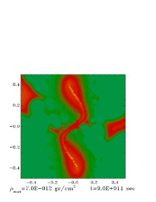
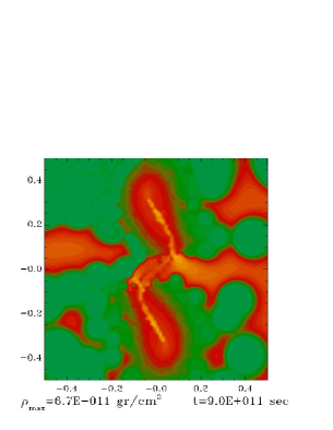
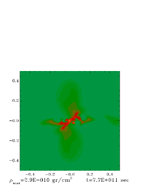
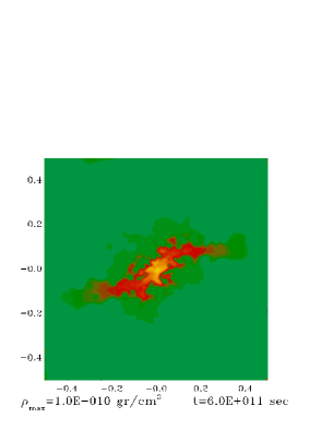
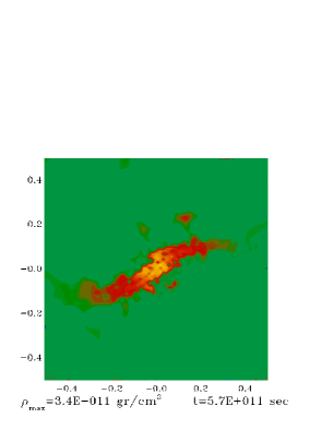
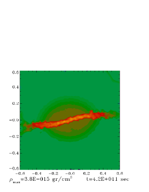
Figure 5: Isodensity plots for the last available snapshot in the head-on collision models $HO-1$ (top left panel), $HO-2$ (top middle panel), $HO-3$ (top right panel), $HO-6$ (bottom left panel), $HO-5$ (bottom middle panel), and $HO-7$ (bottom right panel).

Figure 6: Velocity field of the filament in models $H02$ (top) and $HO6$ (bottom), see the top middle panel and bottom left panel of Fig. 5, respectively.

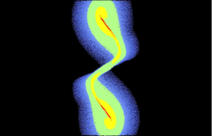
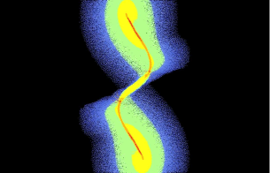
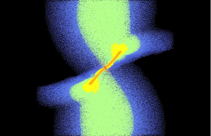
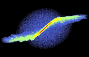
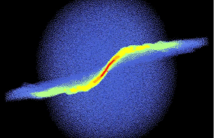
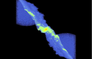
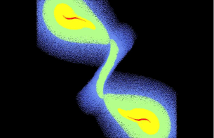
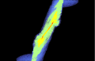
Figure 8: Location of the accretion centers for the last available snapshot of models $HO1$ (first line left), $HO2$ (first line right), $HO3$ (second line left), $HO5$ (second line right), $HO6$ (third line left), $M22$ (third line right), $M3$ (fourth line left), and $M4$ (fourth line right). The colors are a density scale for $\log_{10}\left(\frac{\rho}{\rho_{0}}\right)$ according with the following ranges: blue ( $<2$), green ($2-3$), yellow ($3-4$), orange ($4-5$) and red ($>5$).

Table 1: The collision models.

Model	$\frac{b}{R_{0}}$	$\frac{V_{app}}{c_{0}}$	$N_{acc}$	$Np_{acc}$	$M_{av}/M_{\odot}$	$\rho_{max}\;[gr/cm^{3}]$
MCmR	–	–	27	52	$5.80\times 10^{-5}$	$1.17\times 10^{-10}$
HO-1	0	0.23	80	22	$1.97\times 10^{-5}$	$7.05\times 10^{-12}$
HO-2	0	0.46	29	5	$4.20\times 10^{-6}$	$6.7\times 10^{-11}$
HO-3	0	0.92	30	6	$5.0\times 10^{-6}$	$2.8\times 10^{-10}$
HO-5	0	3.9	104	5	$3.9\times 10^{-6}$	$3.37\times 10^{-11}$
HO-6	0	2.9	37	5	$4.0\times 10^{-6}$	$1.0\times 10^{-10}$
HO-7	0	5.7	9	57	$4.6\times 10^{-5}$	$1.66\times 10^{-13}$
M1	1/4	0.23	210	7	$5.9\times 10^{-6}$	$1.2\times 10^{-11}$
M2	1/2	0.25	103	15	$1.2\times 10^{-5}$	$7.0\times 10^{-12}$
M22	1/2	6.4	42	5	$4.4\times 10^{-6}$	$7.1\times 10^{-11}$
M21	1/2	0.51	214	4	$4.2\times 10^{-6}$	$1.8\times 10^{-11}$
M3	-1/2	0.51	156	5	$4.3\times 10^{-6}$	$1.8\times 10^{-11}$
M4	-1/2	6.4	30	4	$4.0\times 10^{-6}$	$1.2\times 10^{-11}$

Table 2: The evolution and collision time of the collision models.

Model	$t_{evol}/t_{ff}$	$t_{col}/t_{ff}$
HO-1	1.3	12.6
HO-2	1.3	6.3
HO-3	1.1	3.15
HO-5	0.82	0.74
HO-6	0.9	1.0
HO-7	0.75	0.5
M1	1.3	12.6
M2	1.3	12.6
M21	1.3	5.6
M22	0.74	0.45
M3	1.3	5.6
M4	0.92	0.45

References

- [Anathpindika (2009a)] Anathpindika, S. 2009a, A&A, 504, 437.
- [Anathpindika (2009b)] Anathpindika, S. 2009b, A&A, 504, pp.451-460.
- [Anathpindika (2010)] Anathpindika, S. 2010, MNRAS, 405, pp.1431-1443.
- [Arreaga et al. (2007)] Arreaga, G., Klapp, J., Sigalotti, L.G., and Gabbasov, R. 2007, ApJ, 666, 290.
- [Arreaga et al. (2008)] Arreaga, G., Saucedo, J., Duarte, R., and Carmona, J. 2008, Rev. Mex. Astron. Astrophys, 44, 259.
- [Arreaga & Klapp (2010)] Arreaga, G. and Klapp, J. 2010, A&A, 509, A96
- [Bate & Burkert (1997)] Bate, M.R. and Burkert, A., 1997, MNRAS, 288, 1060.
- [Bate et al. (1995)] Bate, M.R., Bonnell, I.A. and Price, M.N., 1995, MNRAS, 277, pp.362-376.
- [Bergin & Tafalla (2007)] Bergin, E. and Tafalla, M. 2007, Annu. Rev. Astro. Astrophys., 45, 339.
- [Balsara (1995)] Balsara, D. 1995, J. Comput. Phys., 121, 357.
- [Bekki et al. (2004)] Bekki, K., Beasley, M., Forbes, D., and Couch, W.J. 2004, ApJ, 602, 730.
- [Bodenheimer et al. (2000)] Bodenheimer, P., Burkert, A., Klein, R.I., & Boss, A.P. 2000, in Protostars and Planets IV, Eds. V.G. Mannings, A.P. Boss and S.S. Russell, University of Arizona Press, Tucson.
- [Burkert & Alves (2009)] Burkert, A. and Alves, J. 2009, ApJ, 695, 1308.
- [Boss et al. (2000)] Boss, A.P., Fisher, R.T., Klein, R. and McKee, C.F. 2000, ApJ, 528, 325.
- [Churchwell et al. (2006)] Churchwell, E., Povich, M.S., Allen, D., Taylor, M.G., Meade, M.R., Babler, B.L., Indebetouw, R., Watson, C., Whitney, B.A., Wolfire, M.G., Bania, T.M., Benjamin, R.A., Clemens, D.P., Cohen, M., Cyganowski, C.J., Jackson, J.M., Kobulnicky, H.A., Mathis, J.S., Mercer, E.P., Stolovy, S.R., Uzpen, B., Watson, D.F. and Wolff,M.J., 2006, ApJ, 649, 759-778.
- [Clark & Bonnell (2006)] Clark, P.C and Bonnell, I.A., 2006, MNRAS, 368, pp.1787-1795.
- [Duarte-Cabral et al. (2010)] Duarte-Cabral, A., Fuller, G.A., Peretto, N., Hatchell, J., Ladd, E.F., Buckle, J., Richer, J and Graves, S.F., 2000, A&A, 519, 27.
- [Federrath et al. (2010)] Federrath, C., Banerjee, R., Clark, P.C. and Klessen, R.S., 2010, ApJ, 713, pp. 269-290.
- [Federrath & Klessen (2012)] Federrath, C. and Klessen, R.S., 2012, ApJ, 761, pp. 156.
- [Furukawa et al. (2009)] Furukawa, N., Dawson, J.R., Ohama, A., Kawamura, A., Mizuno, T and Fukui, Y., 2009, ApJ, 696, pp. L115.
- [Gomez et al. (2007)] Gomez, G.C., Vazquez-Semanedi, E., Shadmehri, M and Ballesteros-Paredes, J., 2007, ApJ, 669, pp. 1042-1049.
- [Graves et al. (2010)] Graves, S. F.; Richer, J. S.; Buckle, J. V.; Duarte-Cabral, A.; Fuller, G. A.; Hogerheijde, M. R.; Owen, J. E.; Brunt, C.; Butner, H. M.; Cavanagh, B.; Chrysostomou, A.; Curtis, E. I.; Davis, C. J.; Etxaluze, M.; Francesco, J. Di; Friberg, P.; Friesen, R. K.; Greaves, J. S.; Hatchell, J.; Johnstone, D.; Matthews, B.; Matthews, H.; Matzner, C. D.; Nutter, D.; Rawlings, J. M. C.; Roberts, J. F.; Sadavoy, S.; Simpson, R. J.; Tothill, N. F. H.; Tsamis, Y. G.; Viti, S.; Ward-Thompson, D.; White, G. J.; Wouterloot, J. G. A.; Yates, J. ,2010, MNRAS, 409, pp. 1412-1428.
- [Hausman (1978)] Hausman, M.A. 1978, ApJ, 245, 72.
- [Heitsch et al. (2008)] Heitsch, F., Hartmann, L.W., Slyz, A.D., Devriendt, J.E.G., and Burkert, A. 2008, ApJ, 674, 316.
- [Jijina et al.(1999)] Jijina, J., Myers, P.C. and Adams, F.C., 1999, ApJ Supplement Series, 125, 161-236.
- [Kimura & Tosa (1996)] Kimura, T. and Tosa, M. 1996, A&A, 308, 979.
- [Kitsionas & Whitworth (2007)] Kitsionas, S. and Whitworth, A.P., 2007, MNRAS, 378, 507-524.
- [Klein & Woods (1998)] Klein, R.I.and Woods, D.T. 1998, ApJ, 497, 777.
- [Klessen & Burkert (2000)] Klessen, R.S. and Burkert, A., 2000, ApJS, 128, 1, pp.287-319.
- [Larson (1981)] Larson, R. 1981, MNRAS, 194, 809.
- [Lattanzio et al. (1985)] Lattanzio, J.C., Monaghan, J.J., Pongracic, H. and Schwarz, M.P. 1985, MNRAS, 215, 125.
- [Marinho & Lepine (2000)] Marinho, E.P. and Lepine, J.R.D. 2000, A&A Suppl., 142, 165.
- [Monaghan & Gingold (1983)] Monaghan, J.J. and Gingold, R.A. 1983, J. Comput. Phys., 52, 374.
- [Motte et al. (1998)] Motte, F., André, P and Neri, R. 1998, Astro.Astrophys, 336, 150-172.
- [Nelson & Papaloizou (1994)] Nelson, R.P. and Papaloizou, C.B., 1994, MNRAS, 270, pp.1-20.
- [Padoan et al.(2014)] Padoan,P., Federrath, C., Chabrier, G., Evans, N.J. II, Johnstone, D., Jorgensen, J.K., McKee, C.F. and Nordlund, A., 2014, Protostars and Planets VI, Beuther, H., Klessen, R.S., Dullemond, C.P. and Henning, T., (eds). University of Arizona Press, Tucson, 914.pp.-pp.77-100.
- [Sigalotti & Klapp (2001a)] Sigalotti, L.G. and Klapp, J. 2001, International Journal of Modern Physics D, 10, 115.
- [Sigalotti & Klapp (2001b)] Sigalotti, L.G. and Klapp, J. 2001, A& A, 378, 165-179.
- [Scoville et al. (1986)] Scoville, N.Z., Sanders, D.B. and Clemens, D.P. 1986, ApJ, 310, L77.
- [Springel (2005)] Springel, V. 2005, MNRAS, 364, 1105.
- [Tackenberg et al.(2014)] Tackenberg, J. , Beuther, H., Henning, T. , Linz, H., Sakai, T., Ragan, S.E., Krause, O., Nielbock, M. Hennemann, M., Pitann, J. and Schmiedeke1, A.,2014, arXiv.1402.0021, accepted by A& A.
- [Tafalla et al.(2004)] Tafalla, M., Myers, P.C., Caselli, P. and Walmsley, C.M.. 2004, A& A , 416, 191.
- [Takahira et al.(2014)] Takahira, K., Tasker, E.J. and Habe, A., 2014, ApJ, 792, issue 1. or seen at arXiv:1407.4544.
- [Testi et al.(2000)] Testi, L., Anneila, I. S., Luca, O. and Onello, J.S.,2000, ApJ , 540, pp. L53-L56.
- [Torii et al.(2011)] Torii, K., Enokiya, R., Sano, H., Yoshiike, S., Kanaoka, N., Ohama, A., Furukawa, N., Dawson, J.R., Moribe, N., Oishi, K., Nakashima, Y., Okuda, T., Yamamoto, H., Kawamura, A., Mizuno, N., Maezawa, H., Onishi, T., Mizuno, A. and Fukui, Y., 2011, ApJ, 738,46.
- [Truelove et al. (1997)] Truelove, J.K., Klein, R.I., McKee, C.F., Holliman, J.H., Howell, L.H., and Greenough, J.A., 1997, ApJ, 489, L179.
- [Vazquez-Semanedi et al. (2007)] Vazquez-Semanedi, E., Gomez, G.C., Jappsen,A.K., Ballesteros-Paredes, J., Gonzalez, R. and Klessen, R.S., 2007, ApJ, 657, pp. 870-883.
- [Vishniac (1983)] Vishniac, E.T. 1983, ApJ, 274, 152.
- [Vishniac (1994)] Vishniac, E.T. 1994, ApJ, 428, 186.
- [Wang et al. (2004)] Wang, J.J., Chen, W.P., Miller, M., Qin, S.L., and Wu, Y.F. 2004, ApJ, 614, L105.
- [Whitehouse & Bate (2006)] Whitehouse, S.C. and Bate, M.R. 2006, MNRAS, 367, 32
- [Whithworth & Ward-Thompson (2001)] Whithworth, A.P. and Ward-Thompson, D. 2001, ApJ, 547, 317
- [Whithworth & Pongracic (1991)] Whithworth, A.P., and Pongracic, H. 1991,in Fragmentation of molecular clouds and star formation, Eds. E. Falgarone, F. Boulangeer and G. Duvert, International Astronomical Union, Kluwer, pp. 523.
- [Zinnecker & Yorke (2007)] Zinnecker, H. and Yorke, H.W., (2007) , Ann. Rev. A& A, 45, 481.