A Model for Competition for Ribosomes in the Cell

Abstract

A single mammalian cell includes an order of $10^{4}-10^{5}$ mRNA molecules and as many as $10^{5}-10^{6}$ ribosomes. Large-scale simultaneous mRNA translation and the resulting competition for the available ribosomes has important implications to the cell’s functioning and evolution. Developing a better understanding of the intricate correlations between these simultaneous processes, rather than focusing on the translation of a single isolated transcript, should help in gaining a better understanding of mRNA translation regulation and the way elongation rates affect organismal fitness. A model of simultaneous translation is specifically important when dealing with highly expressed genes, as these consume more resources. In addition, such a model can lead to more accurate predictions that are needed in the interconnection of translational modules in synthetic biology.

We develop and analyze a general model for large-scale simultaneous mRNA translation and competition for ribosomes. This is based on combining several ribosome flow models (RFMs) interconnected via a pool of free ribosomes. We prove that the compound system always converges to a steady-state and that it always entrains or phase locks to periodically time-varying transition rates in any of the mRNA molecules. We use this model to explore the interactions between the various mRNA molecules and ribosomes at steady-state. We show that increasing the length of an mRNA molecule decreases the production rate of all the mRNAs. Increasing any of the codon translation rates in a specific mRNA molecule yields a local effect: an increase in the translation rate of this mRNA, and also a global effect: the translation rates in the other mRNA molecules all increase or all decrease. These results suggest that the effect of codon decoding rates of endogenous and heterologous mRNAs on protein production is more complicated than previously thought.

I Introduction

Various processes in the cell utilize the same finite pool of available resources. This means that the processes actually compete for these resources, leading to an indirect coupling between the processes. This is particularly relevant when many identical intracellular processes, all using the same resources, take place in parallel.

Biological evidence suggests that the competition for RNA polymerase (RNAP) and ribosomes, and various transcription and translation factors, is a key factor in the cellular economy of gene expression. The limited availability of these resources is one of the reasons why the levels of genes, mRNA, and proteins produced in the cell do not necessarily correlate [63, 32, 57, 67, 53, 69, 29].

It was estimated that in a yeast cell there are approximately $60,000$ mRNA molecules. These can be translated in parallel [74, 71], with possibly many ribosomes scanning the same transcript concurrently. The number of ribosomes is limited (in a yeast cell it is approximately $240,000$) and this leads to a competition for ribosomes. For example, if more ribosomes bind to a certain mRNA molecule then the pool of free ribosomes in the cell is depleted, and this may lead to lower initiation rates in the other mRNAs (see Fig. 1).

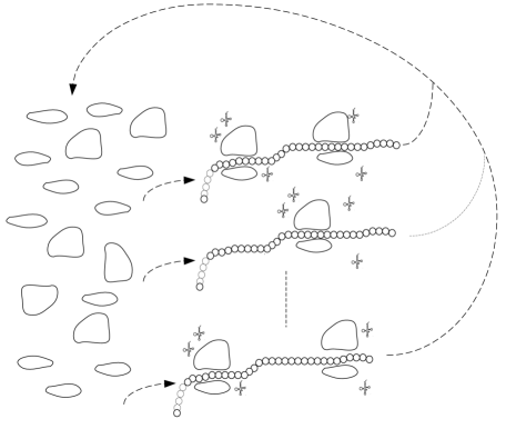
Figure 1: Illustration of simultaneous translation of mRNA chains (right) interconnected via a pool of free ribosomes (left).

There is a growing interest in computational or mathematical models that take into account the competition for available resources in translation and/or transcription (see, for example, [22, 23, 44, 9, 14, 7]). One such model, that explicitly considers the movement of the ribosomes [RNAP] along the mRNA [DNA], is based on a set of asymmetric simple exclusion processes (ASEPs) interconnected to a pool of free ribosomes. ASEP is an important model from non-equilibrium statistical physics describing particles that hop randomly from one site to the next along an ordered lattice of sites, but only if the next site is empty. This form of “rough exclusion” models the fact that the particles cannot overtake one another. ASEP has been used to model and analyze numerous multiagent systems with local interactions including the flow of ribosomes along the mRNA molecule [38],[58]. In this context, the lattice represents the mRNA molecule, and the particles are the ribosomes. For more on mathematical and computational models of translation, see the survey paper [70].

Ref. [24] considered a closed system composed of a single ASEP connected to a pool (or reservoir) of “free” particles. The total number of particles is conserved. This is sometimes referred to as the parking garage problem, with the lattice modeling a road, the particles are cars, and the pool corresponds to a parking garage. Ref. [12] studied a similar system using domain wall theory. Ref. [13] (see also [21]) considered a network composed of two ASEPs connected to a finite pool of particles. The analysis in these papers focuses on the phase diagram of the compound system with respect to certain parameters, and on how the phase of one ASEP affects the phase of the other ASEPs. These studies rely on the phase diagram of a single ASEP that is well-understood only in the case where all the transition rates inside the chain (the elongation rates) are equal. Thus, the network is typically composed of homogeneous ASEPs. Another model [7] combines non-homogenous ASEPs in order to study competition between multiple species of mRNA molecules for a pool of tRNA molecules. This study was based on the Saccharomyces cerevisiae genome. However, in this case (and similar models, such as [14]) analysis seems intractable and one must resort to simulations only.

Our approach is based on the ribosome flow model (RFM) [52]. This is a deterministic, continuous-time, synchronous model for translation that can be derived via the mean-field approximation of ASEP [6]. The RFM includes $n$ state-variables describing the ribosomal density in $n$ consecutive sites along the mRNA molecule, and $n+1$ positive parameters: the initiation rate $\lambda_{0}$, and the elongation rate $\lambda_{i}$ from site $i$ to site $i+1$, $i=1,\dots,n$. The RFM has a unique equilibrium point $e=e(\lambda_{0},\dots,\lambda_{n})$, and any trajectory emanating from a feasible initial condition converges to $e$ [42] (see also [39]). This means that the system always converges to a steady-state ribosomal density that depends on the rates, but not on the initial condition. In particular, the production rate converges to a steady-state value $R$. The mapping from the rates to $R$ is a concave function, so maximizing $R$ subject to a suitable constraint on the rates is a convex optimization problem [48, 73]. Sensitivity analysis of the RFM with respect to the rates has been studied in [49]. These results are important in the context of optimizing the protein production rate in synthetic biology. Ref. [39] has shown that when the rates $\lambda_{i}$ are time-periodic functions, with a common minimal period $T$, then every state-variable converges to a periodic solution with period $T$. In other words, the ribosomal densities entrain to periodic excitations in the rates (due e.g. to periodically-varying abundances of tRNA molecules).

In ASEP with periodic boundary conditions a particle that hops from the last site returns to the first one. The mean field approximation of this model is called the ribosome flow model on a ring (RFMR). The periodic boundary conditions mean that the total number of ribosomes is conserved. Ref. [51] analyzed the RFMR using the theory of monotone dynamical systems that admit a first integral.

Both the RFM and the RFMR model mRNA translation on a single mRNA molecule. In this paper, we introduce a new model, called the RFM network with a pool (RFMNP), that includes a network of RFMs, interconnected through a dynamical pool of free ribosomes, to model and analyze simultaneous translation and competition for ribosomes in the cell. To the best of our knowledge, this is the first study of a network of RFMs. The total number of ribosomes in the RFMNP is conserved, leading to a first integral of the dynamics. Applying the theory of monotone dynamical systems that admit a first integral we prove several mathematical properties of the RFMNP: it admits a continuum of equilibrium points, every trajectory converges to an equilibrium point, and any two solutions emanating from initial conditions corresponding to an equal number of ribosomes converge to the same equilibrium point. These results hold for any set of rates and in particular when the RFMs in the network are not necessarily homogeneous. These stability results are important because they provide a rigorous framework for studying questions such as how does a change in one RFM affects the behavior of all the other RFMs in the network? Indeed, since a steady-state exists, this can be reduced to asking how does a change in one RFM in the network affects the steady-state behavior of the network?

To analyze competition for ribosomes, we consider the effect of increasing one of the rates in one RFM, say RFM #1. This means that the ribosomes traverse RFM #1 more quickly. We show that this always leads to an increase in the production rate of RFM #1. All the other RFMs are always affected in the same manner, that is, either all the other production rates increase or they all decrease. Our analysis shows that this can be explained as follows. Increasing the rate $\lambda_{i}$ in RFM $\#1$ tends to increase the steady-state density in sites $i+1,i+2,\dots$, and decrease the density in site $i$ of this RFM. The total density (i.e., the sum of all the densities on the different sites along RFM $\#1$) can either decrease or increase. In the first case, more ribosomes are freed to the pool, and this increases the initiation rates in all the other RFMs leading to higher production rates. The second case leads to the opposite result. The exact outcome of increasing one of the rates thus depends on the many parameter values defining the pool and the set of RFMs in the network.

Our model takes into account the dynamics of the translation elongation stage, yet is still amenable to analysis. This allows to develop a rigorous understanding of the effect of competition for ribosomes. Previous studies on this topic were either based on simulations (see, for example, [14, 7]) or did not include a dynamical model of translation elongation (see, e.g., [23, 9]). For example, in an interesting paper, combining mathematical modeling and biological experiments, Gyorgy et al. [23] study the expression levels of two adjacent reporter genes on a plasmid in E. coli based on measurements of fluorescence levels, that is, protein levels. These are of course the result of all the gene expression steps (transcription, translation, mRNA degradation, protein degradation) making it difficult to separately study the effect of competition for ribosomes or to study specifically the translation elongation step. Their analysis yields that the attainable output $p_{1},p_{2}$ of the two proteins satisfies the formula

$$\alpha p_{1}+\beta p_{2}=Y,$$ (1)

where $Y$ is related to the total number of ribosomes (but also other translation factors and possibly additional gene expression factors), and $\alpha,\beta$ are constants that depend on parameters such as the plasmid copy number, dissociation constants of the ribosomes binding to the Ribosomal Binding Site (RBS), etc. This equation implies that increasing the production of one protein always leads to a decrease in the production of the other protein (although more subtle correlations may take place via the effects on the constants $\alpha$ and $\beta$). A similar conclusion has been derived for other models as well [16, Ch. 7].

In our model, improving the translation rate of a codon in one mRNA may either increase or decrease the translation rates of all other mRNAs in the cell. Indeed, the effect on the other genes depends on the change in the total density of ribosomes on the modified mRNA molecule, highlighting the importance of modeling the dynamics of the translation elongation step. We show however that when increasing the initiation rate in an RFM in the network, the total density in this RFM always increases and, consequently, the production rate in all the other RFMs decreases. This special case agrees with the results in [23].

Another recent study [50] showed that the hidden layer of interactions among genes arising from competition for shared resources can dramatically change network behavior. For example, a cascade of activators can behave like an effective repressor, and a repression cascade can become bistable. This agrees with several previous studies in the field (see, for example, [29, 2]).

The remainder of this paper is organized as follows. The next section describes the new model. We demonstrate using several examples how it can be used to study translation at the cell level. Section III describes our main theoretical results, and details their biological implications. To streamline the presentation, the proofs of the results are placed in the Appendix. The final section concludes and describes several directions for further research.

II The model and some examples

Since our model is based on a network of interconnected RFMs, we begin with a brief review of the RFM.

II-A Ribosome flow model

The RFM models the traffic flow of ribosomes along the mRNA. The mRNA chain is divided into a set of $n$ compartments or sites, where each site may correspond to a codon or a group of codons. The state-variable $x_{i}(t)$, $i=1,\dots,n$, describes the ribosome occupancy at site $i$ at time $t$, normalized such that $x_{i}(t)=0$ [$x_{i}(t)=1$] implies that site $i$ is completely empty [full] at time $t$. Roughly speaking, one may also view $x_{i}(t)$ as the probability that site $i$ is occupied at time $t$. The dynamical equations of the RFM are:

$$\dot{x}_{1} =\lambda_{0}(1-x_{1})-\lambda_{1}x_{1}(1-x_{2}),$$

$$\dot{x}_{2} =\lambda_{1}x_{1}(1-x_{2})-\lambda_{2}x_{2}(1-x_{3}),$$

$$\dot{x}_{3} =\lambda_{2}x_{2}(1-x_{3})-\lambda_{3}x_{3}(1-x_{4}),$$

$$\vdots$$

$$\dot{x}_{n-1} =\lambda_{n-2}x_{n-2}(1-x_{n-1})-\lambda_{n-1}x_{n-1}(1-x_{n}),$$

$$\dot{x}_{n} =\lambda_{n-1}x_{n-1}(1-x_{n})-\lambda_{n}x_{n}.$$ (2)

These equations describe the movement of ribosomes along the mRNA chain. The transition rates $\lambda_{0},\dots,\lambda_{n}$ are all positive numbers (units=1/time). To explain this model, consider the equation $\dot{x}_{2}=\lambda_{1}x_{1}(1-x_{2})-\lambda_{2}x_{2}(1-x_{3})$. The term $\lambda_{1}x_{1}(1-x_{2})$ represents the flow of particles from site $1$ to site $2$. This is proportional to the occupancy $x_{1}$ at site $1$ and also to $1-x_{2}$, i.e. the flow decreases as site $2$ becomes fuller. In particular, if $x_{2}=1$, i.e. site $2$ is completely full, the flow from site $1$ to site $2$ is zero. This is a “soft” version of the rough exclusion principle in ASEP. Note that the maximal possible flow rate from site $1$ to site $2$ is the transition rate $\lambda_{1}$. The term $\lambda_{2}x_{2}(1-x_{3})$ represents the flow of particles from site $2$ to site $3$.

The dynamical equations for the other state-variables are similar. Note that $\lambda_{0}$ controls the initiation rate into the chain, and that

$$R(t):=\lambda_{n}x_{n}(t),$$

is the rate of flow of ribosomes out of the chain, that is, the translation (or protein production) rate at time $t$. The RFM topology is depicted in Fig. 2.

Figure 2: Topology of the RFM. State variable $x_{i}(t)\in[0,1]$ describes the normalized ribosome occupancy level in site $i$ at time $t$. The initiation rate is $\lambda_{0}$, and $\lambda_{i}$ is the elongation rate between sites $i$ and $i+1$. Production rate at time $t$ is $R(t):=\lambda_{n}x_{n}(t)$.

The RFM encapsulates simple exclusion and unidirectional movement along the lattice just as in ASEP. This is not surprising, as the RFM can be derived via a mean-field approximation of ASEP (see, e.g., [6, p. R345] and [62, p. 1919]). However, the analysis of these two models is quite different as the RFM is a deterministic, continuous-time, synchronous model, whereas ASEP is a stochastic, discrete-type, asynchronous one.

In order to study a network of interconnected RFMs, it is useful to first extend the RFM into a single-input single-output (SISO) control system:

$$\dot{x}_{1} =\lambda_{0}(1-x_{1})u-\lambda_{1}x_{1}(1-x_{2}),$$

$$\dot{x}_{2} =\lambda_{1}x_{1}(1-x_{2})-\lambda_{2}x_{2}(1-x_{3}),$$

$$\dot{x}_{3} =\lambda_{2}x_{2}(1-x_{3})-\lambda_{3}x_{3}(1-x_{4}),$$

$$\vdots$$

$$\dot{x}_{n-1} =\lambda_{n-2}x_{n-2}(1-x_{n-1})-\lambda_{n-1}x_{n-1}(1-x_{n}),$$

$$\dot{x}_{n} =\lambda_{n-1}x_{n-1}(1-x_{n})-\lambda_{n}x_{n},$$

$$y =\lambda_{n}x_{n}.$$ (3)

Here the translation rate becomes the output $y$ of the system, and the flow into site $1$ is multiplied by a time-varying control $u:\mathbb{R}_{+}\to\mathbb{R}_{+}$, representing the flow of ribosomes from the “outside world” into the strand which is related to the rate ribosomes diffuse to the 5’end (in eukaryotes) or the RBS (in prokaryotes) of the mRNA. Of course, mathematically one can absorb $\lambda_{0}$ into $u$, but we do not do this because we think of $\lambda_{0}$ as representing some local/mRNA-specific features of the mRNA sequence (e.g. the strength of the Kozak sequences in eukaryotes or the RBS in prokaryote).

The set of admissible controls $\mathcal{U}$ is the set of bounded and measurable functions taking values in $\mathbb{R}_{+}$ for all time $t\geq 0$. Eq. (II-A), referred to as the RFM with input and output (RFMIO) [43], facilitates the study of RFMs with feedback connections. We note in passing that (II-A) is a monotone control system as defined in [4]. From now on we write (II-A) as

$$\dot{x} =f(x,u),$$

$$y =\lambda_{n}x_{n}.$$ (4)

Let

$$C^{n}:=\{z\in\mathbb{R}^{n}:z_{i}\in[0,1],\;i=1,\dots,n\},$$

denote the closed unit cube in $\mathbb{R}^{n}$. Since the state-variables represent normalized occupancy levels, we always consider initial conditions $x(0)\in C^{n}$. It is straightforward to verify that $C^{n}$ is an invariant set of (II-A), i.e. for any $u\in\mathcal{U}$ and any $x(0)\in C^{n}$ the trajectory satisfies $x(t,u)\in C^{n}$ for all $t\geq 0$.

II-B RFM network with a pool

To model competition for ribosomes in the cell, we consider a set of $m\geq 1$ RFMIOs, representing $m$ different mRNA chains. The $i$th RFMIO has length $n_{i}$, input function $u^{i}$, output function $y^{i}$, and rates $\lambda^{i}_{0},\dots,\lambda^{i}_{n_{i}}$. The RFMIOs are interconnected through a pool of free ribosomes (i.e., ribosomes that are not attached to any mRNA molecule). The output of each RFMIO is fed into the pool, and the pool feeds the initiation locations in the mRNAs (see Fig. 3). Thus, the model includes $m$ RFMIOs:

$$\dot{x}^{1} =f(x^{1},u^{1}),\quad y^{1}=\lambda^{1}_{n_{1}}x_{n_{1}},$$

$$\vdots$$

$$\dot{x}^{m} =f(x^{m},u^{m}),\quad y^{m}=\lambda^{m}_{n_{m}}x_{n_{m}},$$ (5)

and a dynamic pool of ribosomes described by

$$\dot{z}=\sum_{j=1}^{m}y^{j}-\sum_{j=1}^{m}\lambda^{j}_{0}(1-x_{1}^{j})G_{j}(z).$$ (6)

where $z:\mathbb{R}_{+}\to\mathbb{R}$ describes the pool occupancy. Eq. (6) means that the flow into the pool is the sum of all output rates $\sum_{j=1}^{m}y^{j}$ of the RFMIOs minus the total flow of ribosomes that bind to an mRNA molecule $\sum_{j=1}^{m}\lambda^{j}_{0}(1-x_{1}^{j})G_{j}(z)$. Recall that the term $(1-x_{1}^{j})$ represents the exclusion, i.e. as the first site in RFMIO $\#j$ becomes fuller, less ribosomes can bind to it. Thus, the input to RFMIO $\#j$ is

$$u^{j}(t)=G_{j}(z(t)),\quad j=1,\dots,m.$$ (7)

We assume that each $G_{j}(\cdot):\mathbb{R}_{+}\to\mathbb{R}_{+}$ satisfies: (1) $G_{j}(0)=0$; $G_{j}$ is continuously differentiable and $G_{j}^{\prime}(z)>0$ for all $z\geq 0$ (so $G_{j}$ is strictly increasing on $\mathbb{R}_{+}$); and (3) there exists $s>0$ such that $G_{j}(z)\leq sz$ for all $z>0$ sufficiently small. These properties imply in particular that if the pool is empty then no ribosomes can bind to the mRNA chains, and that as the pool becomes fuller the initiation rates to the RFMIOs increase.

Typical examples for functions satisfying these properties include the linear function, say, $G_{j}(z)=z$, and $G_{j}(z)=a_{j}\tanh(b_{j}z)$, with $a_{j},b_{j}>0$. In the first case, the flow of ribosomes into the first site of RFM $\#i$ is given by $\lambda^{i}_{0}z(1-x^{i}_{1})$, and the product here can be justified via mass-action kinetics. The use of $\tanh$ may be suitable for modeling a saturating function. This is in fact a standard function in ASEP models with a pool [13, 1], because it is zero when $z$ is zero, uniformly bounded, and strictly increasing for $z\geq 0$. Also, for $z\geq 0$ the function $\tanh(z)$ takes values in $[0,1)$ so it can also be interpreted as a probability function [20].

In the context of a shared pool, it is natural to consider the special case where $G_{j}(z)=G(z)$ for all $j=1,\dots,m$. The differences between the initiation sites in the strands are then modeled by the different $\lambda_{0}^{j}$’s.

Note that combining the properties of $G_{j}$ with (6) implies that if $z(0)\geq 0$ then $z(t)\geq 0$ for all $t\geq 0$. Thus, the pool occupancy is always non-negative.

Summarizing, the RFM network with a pool (RFMNP) is given by equations (II-B), (6), and (7). This is a dynamical system with $d:=1+\sum_{i=1}^{m}n_{i}$ state-variables.

Figure 3: Topology of the RFMNP.

Example 1

Consider a network with $m=2$ RFMIOs, the first [second] with dimension $n_{1}=2$ [$n_{2}=3$]. Then the RFMNP is given by

$$\dot{x}^{1}_{1} =\lambda^{1}_{0}(1-x_{1}^{1})G_{1}(z)-\lambda_{1}^{1}x_{1}^{1}(1-x_{2}^{1}),$$

$$\dot{x}^{1}_{2} =\lambda^{1}_{1}x^{1}_{1}(1-x^{1}_{2})-\lambda_{2}^{1}x_{2}^{1},$$

$$\dot{x}_{1}^{2} =\lambda^{2}_{0}(1-x_{1}^{2})G_{2}(z)-\lambda_{1}^{2}x_{1}^{2}(1-x_{2}^{2}),$$

$$\dot{x}_{2}^{2} =\lambda_{1}^{2}x_{1}^{2}(1-x_{2}^{2})-\lambda_{2}^{2}x_{2}^{2}(1-x_{3}^{2}),$$

$$\dot{x}_{3}^{2} =\lambda_{2}^{2}x_{2}^{2}(1-x_{3}^{2})-\lambda_{3}^{2}x_{3}^{2},$$

$$\dot{z} =\lambda_{2}^{1}x_{2}^{1}+\lambda_{3}^{2}x_{3}^{2}-\lambda^{1}_{0}(1-x_{1}^{1})G_{1}(z)-\lambda^{2}_{0}(1-x_{1}^{2})G_{2}(z).$$ (8)

Note that this system has $d=6$ state-variables. $\square$

An important property of the RFMNP is, that being a closed system, the total occupancy

$$H(t):=z(t)+\sum_{j=1}^{m}\sum_{i=1}^{n_{j}}x^{j}_{i}(t),$$ (9)

is conserved, that is,

$$H(t)\equiv H(0),\quad\text{for all }t\geq 0.$$ (10)

In other words, $H$ is a first integral of the dynamics. In particular, this means that $z(t)\leq H(t)=H(0)$ for all $t\geq 0$, i.e. the pool occupancy is uniformly bounded.

The RFMNP models mRNAs that compete for ribosomes because the total number of ribosomes is conserved. As more ribosomes bind to the RFMs, the pool depletes, $G_{j}(z)$ decreases, and the effective initiation rate to all the RFMs decreases. This allows to systematically address important biological questions on large-scale simultaneous translation under competition for ribosomes. The following examples demonstrate this. We prove in Section III that all the state-variables in the RFMNP converge to a steady-state. Let $e^{i}_{j}\in[0,1]$ denote the steady-state occupancy in site $j$ in RFMIO $\#i$, and let $e_{z}\in[0,\infty)$ denote the steady-state occupancy in the pool. In the examples below we always consider these steady-state values (obtained numerically by simulating the differential equations).

Example 2

Although we are mainly interested in modeling large-scale simultaneous translation, it is natural to first consider a model with a single mRNA molecule connected to a pool of ribosomes. From a biological perspective, this models the case where there is one gene that is highly expressed with respect to all other genes (e.g. an extremely highly expressed heterologous gene).

Consider an RFMNP that includes a single RFMIO (i.e. $m=1$), with dimension $n_{1}=3$, rates $\lambda^{1}_{i}=1$, $i=0,1,2,3$, and a pool with output function $G(z)=\tanh(z)$. We simulated this system for the initial condition $x^{1}_{i}(0)=0$, $z(0)=c$ for various values of $c$. Note that $H(t)\equiv H(0)=c$. Fig. 4 depicts the steady-state values $e_{1},e_{2},e_{3}$ of the state-variables in the RFMIO, and the steady-state pool occupancy $e_{z}$. It may be seen that for small values of $c$ the steady-state ribosomal densities and thus the production rates are very low. This is simply because there are not enough ribosomes in the network. The ribosomal densities increase with $c$. For large values of $c$, the output function of the pool saturates, as $\tanh(z)\to 1$, and so does the initiation rate in the RFMIO. Thus, the densities in the RFMIO saturate to the values corresponding to the initiation rate $\lambda_{0}=1$, and then all the remaining ribosomes accumulate in the pool. Using a different pool output function, for example $G(z)=z$, leads to the same qualitative behavior, but with higher saturation values for the ribosomal densities in the RFMIO. (Note that the ribosomal densities in an RFM are finite even when $\lambda_{0}\to\infty$ [41].) $\square$

This simple example already demonstrates the coupling between the ribosomal pool, initiation rate, and elongation rates. When the ribosomal pool is small the initiation rate is low. Thus, the ribosomal densities on the mRNA are low and there are no interactions between ribosomes (i.e., no “traffic jams”) along the mRNA. The initiation rate becomes the rate limiting step of translation. On the other-hand, when there are many ribosomes in the pool the initiation rate increases, the elongation rates become rate limiting and “traffic jams” along the mRNA evolve. At some point, a further increase in the number of ribosomes in the pool will have a negligible effect on the production rate.

It is known that there can be very large changes in the number of ribosomes in the cell during e.g. exponential growth. For example. Ref. [8] reports changes in the range $6,800$ to $72,000$. The example above demonstrates how these large changes in the number of ribosomes are expected to affect the translational regimes; specifically, it may cause a switch between the different regimes mentioned above.

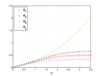
Figure 4: Steady-state values in the RFMNP in Example 2 as a function of the total occupancy $H(0)=c$.

The next example describes an RFMNP with several mRNA chains. Let $1_{n}\in\mathbb{R}^{n}$ denote the vector of $n$ ones.

Example 3

Consider an RFMNP with $m=3$ RFMIOs of dimensions $n_{1}=n_{2}=n_{3}=3$, and rates

$$\lambda^{1}_{i}=c,\quad\lambda^{2}_{i}=5,\quad\lambda^{3}_{i}=10,\quad i=0,\dots,3.$$

In other words, every RFMIO has homogeneous rates. Suppose also that $G_{i}(z)=\tanh(z)$, for $i=1,2,3$. We simulated this RFMNP for different values of $c$ with the initial condition $z(0)=0$, $x^{1}(0)=(1/2)1_{3}$, $x^{2}(0)=(1/3)1_{3}$ and $x^{3}(0)=(1/4)1_{3}$. Thus, $H(0)=3.25$ in all the simulations. For each value of $c$, every state-variable in the RFMNP converges to a steady-state. Fig. 5 depicts the steady-state value $e_{z}$ and the steady-state output $y^{i}$ in each RFMIO. It may be seen that increasing $c$, i.e. increasing all the elongation rates in RFMIO $\#1$ leads to an increase in the steady-state translation rates in all the RFMIOs in the network. Also, it leads to an increase in the steady-state occupancy of the pool. It may seem that this contradicts (10) but this is not so. Increasing $c$ indeed increases all the steady-state translation rates, but it decreases the steady-state occupancies inside each RFMIO so that the total $H(t)=H(0)=3.25$ is conserved.

Define the average steady-state occupancy (ASSO) in RFMIO $\#j$ by $\bar{e}^{j}:=\frac{1}{n_{j}}\sum_{i=1}^{n_{j}}e^{j}_{i}$. Fig. 6 depicts the ASSO in each RFMIO as a function of $c$. It may be seen as $c$ increases the ASSO in RFMIO $\#1$ decreases quickly, yet the ASSOs in the other two RFMIOs slowly increases. Since the ribosomes spend less time on RFMIO $\#1$ (due to increased $c$) they are now available for translating the other RFMIOs, leading to the increased ASSO in the other mRNAs. $\square$

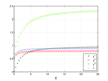
Figure 5: Steady-state outputs $y^{i}$ of the three RFMIOs and pool occupancy $z$ as a function of the homogeneous transition rate $c$ in RFMIO $\#1$.

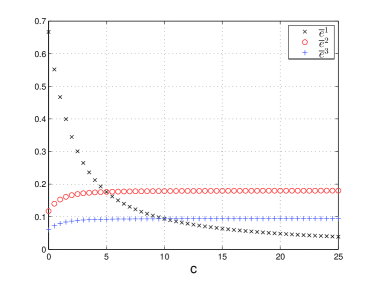
Figure 6: Average steady-state occupancy in the three RFMIOs as a function of the homogeneous transition rate $c$ in RFMIO $\#1$.

From a biological point of view this example corresponds to a situation where accelerating one of the mRNA chains increases the protein production rates in all the mRNAs and also increases the number of free ribosomes. Surprisingly, perhaps, it also suggests that a relatively larger number of free ribosomes in the cell corresponds to higher protein production rates. This agrees with evolutionary, biological, and synthetic biology studies that have suggested that (specifically) highly expressed genes (that are transcribed into many mRNA molecules) undergo selection to include codons with improved elongation rates [32, 66, 63]. Specifically, two mechanisms by which improved codons affect translation efficiency and the organismal fitness are [66]: (1) global mechanism: selection for improved codons contributes toward improved ribosomal recycling and global allocation; the increased number of free ribosomes improves the effective translation initiation rate of all genes, and thus improves global translation efficiency; and (2) local mechanism: the improved translation elongation rate of an mRNA contributes directly to its protein production rate.

The example above demonstrates both mechanisms, as improvement of the translation elongation rates of one RFM increases the translation rate of this mRNA (local translation efficiency), and also of the other RFMs (global translation efficiency). In addition, as can be seen, the decrease in ASSO in RFMIO $\#1$ is significantly higher than the increase in ASSO in the other RFMIO. Thus, the simulation also demonstrates that increasing the translation rate $c$ may contribute to decreasing ribosomal collision (and possibly ribosomal abortion).

We prove in Section III that when one of the rates in one of the RFMIOs increases two outcomes are possible: either all the production rates in the other RFMs increase (as in this example) or they all decrease. As discussed below, we believe that this second case is less likely to occur in endogenous genes, but may occur in heterologous gene expression.

The next example describes the effect of changing the length of one RFMIO in the network.

Example 4

Consider an RFMNP with $m=2$ RFMIOs of dimensions $n_{1}$ and $n_{2}=10$, rates

$$\lambda^{1}_{i} =1,\quad i=0,\dots,n_{1},$$

$$\lambda^{2}_{j} =1,\quad j=0,\dots,10,$$

and $G_{i}(z)=\tanh(z/200)$, $i=1,2$. In other words, both RFMIOs have the same homogeneous rates. We simulated this RFMNP for different values of $n_{1}$ with the initial condition $z(0)=100$, $x^{1}(0)=0_{n_{1}}$, $x^{2}(0)=0_{10}$. Thus $H(0)=100$ in all the simulations. For each value of $n_{1}$, every state-variable in the RFMNP converges to a steady-state. Fig. 7 depicts the steady-state values of $z$, and the steady-state output $y^{i}$ in each RFMIO. It may be seen that increasing $n_{1}$, i.e. increasing the length of RFMIO $\#1$ leads to a decrease in the steady-state production rates and in the steady-state pool occupancy. This is reasonable, as increasing $n_{1}$ means that ribosomes that bind to the first chain remain on it for a longer period of time. This decreases the production rate $y^{1}$ and, by the competition for ribosomes, also decreases the pool occupancy and thus decreases $y^{2}$. $\square$

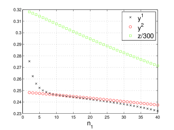
Figure 7: Steady-state outputs $y^{i}$ of the two RFMIOs and steady-state pool occupancy $z/300$ as a function of the length $n_{1}$ of RFMIO $\#1$. The normalization of $z$ by $300$ is used to obtain similar magnitudes for all the values only.

From a biological point of view this suggests that decreasing the length of mRNA molecules contributes locally and globally to improving translation efficiency. A shorter coding sequence improves the translation rate of the mRNA and, by competition, may also improve the translation rates in all other mRNAs. Thus, we should expect to see selection for shorter coding sequences, specifically in highly expressed genes and in organisms with large population size. Indeed, previous studies have reported that in some organisms the coding regions of highly expressed genes tend to be shorter [14]; other studies have shown that other (non-coding) parts of highly expressed genes tend to be shorter [11, 17, 35, 64]. Decreasing the length of different parts of the gene should contribute to organismal fitness via improving the energetic cost of various gene expression steps. For example, shorter genes should improve the metabolic cost of synthesizing mRNA and proteins; it can also reduce the energy spent for splicing and processing of RNA and proteins. However, there are of course various functional and regulatory constraints that also contribute to shaping the gene length (see, for example [10]). Our results and these previous studies suggest that in some cases genes are expected to undergo selection also for short coding regions, as this reduces the required number of translating ribosomes.

The next section describes theoretical results on the RFMNP. All the proofs are placed in the Appendix.

III Mathematical properties of the RFMNP

Let

$$\Omega:=[0,1]^{n_{1}}\times\dots\times[0,1]^{n_{m}}\times[0,\infty)$$

denote the state-space of the RFMNP (recall that every $x_{i}^{j}$ takes values in $[0,1]$ and $z\in[0,\infty)$). For an initial condition $a\in\Omega$, let $\begin{bmatrix}x(t,a)&z(t,a)\end{bmatrix}^{\prime}$ denote the solution of the RFMNP at time $t$. It is straightforward to show that the solution remains in $\Omega$ for all $t\geq 0$. Our first result shows that a slightly stronger property holds.

III-A Persistence

Proposition 1

For any $\tau>0$ there exists $\varepsilon=\varepsilon(\tau)>0$, with $\varepsilon(\tau)\to 0$ when $\tau\to 0$, such that for all $t\geq\tau$, all $j=1,\dots,m$, all $i=1,\dots,n_{j}$, and all $a\in(\Omega\setminus\{0\})$,

$$\varepsilon\leq x^{j}_{i}(t,a)\leq 1-\varepsilon,$$

and

$$\quad\varepsilon\leq z(t,a).$$

In other words, after time $\tau$ the solution is $\varepsilon$-separated from the boundary of $\Omega$. This result is useful because on the boundary of $\Omega$, denoted $\partial\Omega$, the RFMNP looses some desirable properties. For example, its Jacobian matrix may become reducible on $\partial\Omega$. Prop. 1 allows us to overcome this technical difficulty, as it implies that any trajectory is separated from the boundary after an arbitrarily short time.

III-B Strong Monotonicity

Recall that a cone $K\subseteq\mathbb{R}^{n}$ defines a partial order in $\mathbb{R}^{n}$ as follows. For two vectors $a,b\in\mathbb{R}^{n}$, we write $a\leq b$ if $(b-a)\in K$; $a<b$ if $a\leq b$ and $a\not=b$; and $a\ll b$ if $(b-a)\in\operatorname{Int}(K)$. A dynamical system $\dot{x}=f(x)$ is called monotone if $a\leq b$ implies that $x(t,a)\leq x(t,b)$ for all $t\geq 0$. In other words, monotonicity means that the flow preserves the partial ordering [59]. It is called strongly monotone if $a<b$ implies that $x(t,a)\ll x(t,b)$ for all $t>0$.

From here on we consider the particular case where the cone is $K=\mathbb{R}^{n}_{+}$. Then $a\leq b$ if $a_{i}\leq b_{i}$ for all $i$, and $a\ll b$ if $a_{i}<b_{i}$ for all $i$. A system that is monotone with respect to this partial order is called cooperative.

The next result analyzes the cooperativity of the RFMNP. Let $d:={1+\sum\limits_{i=1}^{m}n_{i}}$ denote the dimension of the RFMNP.

Proposition 2

For any $a,b\in\Omega$ with $a\leq b$,

$$x(t,a)\leq x(t,b)\text{ and }z(t,a)\leq z(t,b),\quad\text{for all }t\geq 0.$$ (11)

Furthermore, if $a<b$ then

$$x(t,a)\ll x(t,b)\text{ and }z(t,a)<z(t,b),\quad\text{for all }t>0.$$ (12)

This means the following. Consider the RFMNP initiated with two initial conditions such that the ribosomal densities in every site and the pool corresponding to the first initial condition are smaller or equal to the densities in the second initial condition. Then this correspondence between the densities remains true for all time $t\geq 0$.

III-C Stability

For $s\geq 0$, let

$$L_{s}:=\{y\in\Omega:1_{d}^{\prime}y=s\}.$$

In other words, $L_{s}$ is a level set of the first integral $H$.

Theorem 1

Every level set $L_{s}$, $s\geq 0$, contains a unique equilibrium point $e_{L_{s}}$ of the RFMNP, and for any initial condition $a\in L_{s}$, the solution of the RFMNP converges to $e_{L_{s}}$. Furthermore, for any $0\leq s<p$,

$$e_{L_{s}}\ll e_{L_{p}}.$$ (13)

In particular, this means that every trajectory converges to an an equilibrium point, representing steady-state ribosomal densities in the RFMIOs and the pool. Note that Proposition 1 implies that for any $s>0$, $e_{L_{s}}\in\operatorname{Int}(\Omega)$. Eq. (13) means that the continuum of equilibrium points, namely, $\{e_{L_{s}}:\;s\in[0,\infty)\}$, are linearly ordered.

Example 5

Consider an RFMNP with $m=2$ RFMIOs with dimensions $n_{1}=n_{2}=1$, and $G_{i}(z)=z$, $i=1,2$, i.e.

$$\dot{x}^{1}_{1} =\lambda_{0}^{1}(1-x_{1}^{1})z-\lambda_{1}^{1}x_{1}^{1},$$

$$\dot{x}_{1}^{2} =\lambda_{0}^{2}(1-x_{1}^{2})z-\lambda_{1}^{2}x_{1}^{2},$$

$$\dot{z} =\lambda_{1}^{1}x_{1}^{1}+\lambda_{1}^{2}x_{1}^{2}-\lambda_{0}^{1}(1-x_{1}^{1})z-\lambda_{0}^{2}(1-x_{1}^{2})z.$$ (14)

Note that even in this simple case the RFMNP is a nonlinear system. Assume that $\lambda_{0}^{1}=\lambda_{0}^{2}=1$, and that $\lambda^{1}_{1}=\lambda^{2}_{1}$, and denote this value simply by $\lambda$. Pick an initial condition in $\Omega$, and let $s:=x_{1}^{1}(0)+x_{1}^{2}(0)+z(0)$, so that the trajectory belong to $L_{s}$ for all $t\geq 0$. Any equilibrium point $e=\begin{bmatrix}e_{1}&e_{2}&e_{z}\end{bmatrix}^{\prime}\in L_{s}$ satisfies

$$(1-e_{1})e_{z} =\lambda e_{1},$$

$$(1-e_{2})e_{z} =\lambda e_{2},$$

$$e_{1}+e_{2}+e_{z} =s.$$

This yields two solutions

$$e_{1} =e_{2}=\left(s+2+\lambda-\sqrt{(s+2+\lambda)^{2}-8s}\right)/4,$$ (15)

$$e_{z} =\left(s-2-\lambda+\sqrt{(s+2+\lambda)^{2}-8s}\right)/2,$$

and

$$e_{1} =e_{2}=\left(s+2+\lambda+\sqrt{(s+2+\lambda)^{2}-8s}\right)/4,$$

$$e_{z} =\left(s-2-\lambda-\sqrt{(s+2+\lambda)^{2}-8s}\right)/2,$$

It is straightforward to verify that in the latter solution $e_{z}<0$, so this is not a feasible solution. The solution (15) does belong to $L_{s}$, so the system admits a unique equilibrium in $L_{s}$. Fig. 8 depicts trajectories of (5) for three initial conditions in $L_{1}$, namely, $\begin{bmatrix}1&0&0\end{bmatrix}$, $\begin{bmatrix}0&1&0\end{bmatrix}$, and $\begin{bmatrix}0&1/2&1/2\end{bmatrix}$, and the equilibrium point (15) for $s=\lambda=1$. It may be seen that every one of these trajectories converges to $e$. $\square$

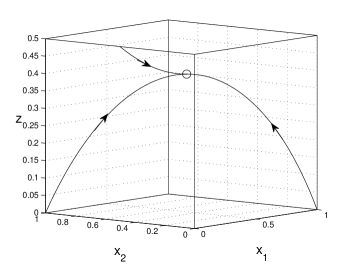
Figure 8: Trajectories of the system in Example 5 for three initial conditions in $L_{1}$. The equilibrium point (15) is marked by a circle.

III-D Contraction

Contraction theory is a powerful tool for analyzing nonlinear dynamical systems (see, e.g., [36]), with applications to many models from systems biology [3, 54, 40]. In a contractive system, the distance between any two trajectories decreases at an exponential rate. It is clear that the RFMNP is not a contractive system on $\Omega$, with respect to any norm, as it admits more than a single equilibrium point. Nevertheless, the next result shows that the RFMNP is non-expanding with respect to the $\ell_{1}$ norm: $|q|_{1}=\sum_{i=1}^{d}|q_{i}|$.

Proposition 3

For any $a,b\in\Omega$,

$$\left|\begin{bmatrix}x(t,a)\\ z(t,a)\end{bmatrix}-\begin{bmatrix}x(t,b)\\ z(t,b)\end{bmatrix}\right|_{1}\leq|a-b|_{1},\quad\text{for all }t\geq 0.$$ (16)

In other words, the $\ell_{1}$ distance between trajectories can never increase.

Pick $a\in\Omega$, and let $s:=1_{d}^{\prime}a$. Substituting $b=e_{L_{s}}$ in (16) yields

$$\left|\begin{bmatrix}x(t,a)\\ z(t,a)\end{bmatrix}-e_{L_{s}}\right|_{1}\leq|a-e_{L_{s}}|_{1},\quad\text{for all }t\geq 0.$$ (17)

This means that the convergence to the equilibrium point $e_{L_{s}}$ is monotone in the sense that the $\ell_{1}$ distance to $e_{L_{s}}$ can never increase. Combining (17) with Theorem 1 implies that every equilibrium point of the RFMNP is semistable [26].

III-E Entrainment

Many important biological processes are periodic. Examples include circadian clocks and the cell cycle division process. Proper functioning requires certain biological systems to follow these periodic patterns, i.e. to entrain to the periodic excitation.

In the context of translation, it has been shown that both the RFM [39] and the RFMR [51] entrain to periodic translation rates, i.e. if all the transition rates are periodic time-varying functions, with a common (minimal) period $T>0$ then each state variable converges to a periodic trajectory, with a period $T$. Here we show that the same property holds for the RFMNP.

We say that a function $f$ is $T$-periodic if $f(t+T)=f(t)$ for all $t$. Assume that the $\lambda^{j}_{i}$’s in the RFMNP are time-varying functions satisfying:

• there exist $0<\delta_{1}<\delta_{2}$ such that $\lambda^{j}_{i}(t)\in[\delta_{1},\delta_{2}]$ for all $t\geq 0$ and all $j\in\{1,\dots,m\}$ , $i\in\{1,\dots,n_{j}\}$.

• there exists a (minimal) $T>0$ such that all the $\lambda^{j}_{i}$’s are $T$-periodic.

We refer to the model in this case as the periodic ribosome flow model network with a pool (PRFMNP).

Theorem 2

Consider the PRFMNP. Fix an arbitrary $s>0$. There exists a unique function $\phi_{s}:\mathbb{R}_{+}\to\operatorname{Int}(\Omega)$, that is $T$-periodic, and for any $a\in L_{s}$ the solution of the PRFMNP converges to $\phi_{s}$.

In other words, every level set $L_{s}$ of $H$ contains a unique periodic solution, and every solution of the PRFMNP emanating from $L_{s}$ converges to this solution. Thus, the PRFMNP entrains (or phase locks) to the periodic excitation in the $\lambda^{j}_{i}$’s. This implies in particular that all the protein production rates converge to a periodic pattern with period $T$.

Note that since a constant function is a periodic function for any $T$, Theorem 2 implies entrainment to a periodic trajectory in the particular case where one of the $\lambda^{j}_{i}$’s oscillates, and all the other are constant. Note also that the stability result in Theorem 1 follows from Theorem 2.

Example 6

Consider the RFMNP (1) with $G_{i}(z)=\tanh(z)$, and all rates equal to one except for $\lambda_{2}^{2}(t)=5+4\sin(2\pi t)$. In other words, there is a single time-varying periodic rate in RFMIO $\#2$. Note that all these rates are periodic with a common minimal period $T=1$. Fig. 9 depicts the solution of this PRFMNP as a function of time $t$ for $16.9\leq t\leq 20$. The initial condition is $z(0)=x^{i}_{j}(0)=1/4$ for all $i,j$. It may be seen that all the state variables converge to a periodic solution. In particular, all state variables $x^{2}_{i}(t)$ converge to a periodic solution with (minimal) period $T=1$, and so does the pool occupancy $z(t)$. The $x^{1}_{j}(t)$’s also converge to a periodic solution, but it is not possible to tell from the figure whether there are small oscillations with period $T=1$ or the convergence is to a constant (of course, in both cases this is a periodic solution with period $T=1$). However, it can be shown using the first two equations in (1) that if $z(t)$ converges to a periodic solution then so do $x^{1}_{1}(t)$ and $x^{1}_{2}(t)$. Note that the peaks in $x^{2}_{3}(t)$ are correlated with dips in $x^{2}_{2}(t)$, this is because when $\lambda^{2}_{2}(t)$ is high on some time interval, i.e. the transition rate from site $2$ to site $3$ is high, there is a high flow of ribosomes from site $2$ to site $3$ during this interval. $\square$

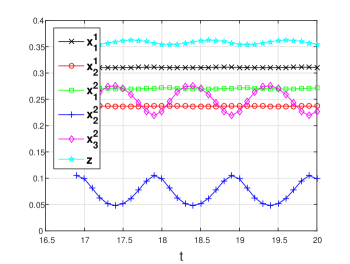
Figure 9: Trajectories of the PRFMNP in Example 6 as a function of time.

From the biophysical point of view this means that the coupling between the mRNA molecules can induce periodic oscillations in all the protein production rates even when all the transition rates in the molecules are constant, except for a single rate in a single molecule that oscillates periodically. The translation rate of codons is affected among others by the tRNA supply (i.e. the intracellular abundance of the different tRNA species) and demand (i.e. total number of codons from each type on all the mRNA molecules) (see for example [47]). Thus, the translation rate of a codon(s) is affected by changes in the demand (e.g. oscillations in mRNA levels) or by changes in the supply (e.g. oscillations in tRNA levels). The results reported here may suggest that oscillations in the mRNA levels of some genes or in the concentration of some tRNA species (that occur for example during the cell cycle [60, 19]), can induce oscillations in the translation rates of the rest of the genes.

III-F Competition

We already know that any trajectory of the RFMNP converges to an equilibrium point. A natural question is how will a change in the parameters (that is, the transition rates) affect this equilibrium point. For example, if we increase some transition rate $\lambda^{j}_{i}$ in RFMIO $\#j$, how will this affect the steady-state production rate in the other RFMIOs? Without loss of generality, we assume that the change is in a transition rate of RFMIO $\#1$.

Theorem 3

Consider an RFMNP with $m$ RFMIOs with dimensions $n_{1},\dots,n_{m}$. Let $\lambda:=\begin{bmatrix}\lambda^{1}_{0}&\dots&\lambda^{m}_{n_{m}}\end{bmatrix}^{\prime}$ denote the set of all parameters of the RFMNP, and let

$$e=\begin{bmatrix}e^{1}_{1}\;\dots\;e^{1}_{n_{1}}\;e^{2}_{1}\;\dots\;e^{2}_{n_{2}}\;\dots\;e^{m}_{1}\;\dots\;e^{m}_{n_{m}}\;e_{z}\end{bmatrix}^{\prime}\in(0,1)^{n_{1}+\dots+n_{m}}\times\mathbb{R}_{++}$$

denote the equilibrium point of the RFMNP on some fixed level set of $H$. Pick $i\in\{0,\dots,n_{1}\}$. Consider the RFMNP obtained by modifying $\lambda^{1}_{i}$ to $\bar{\lambda}^{1}_{i}$, with $\bar{\lambda}^{1}_{i}>\lambda^{1}_{i}$. Let $\bar{e}$ denote the equilibrium point in the new RFMNP and let $\tilde{e}:=\bar{e}-e$. Then

$$\tilde{e}^{1}_{i}<0,\text{ and }\tilde{e}^{1}_{j}>0,\text{ for all }j\in\{i+1,...,n_{1}\},$$ (18)

$$\operatorname{{\mathrm{s}ign}}(\tilde{e}^{i}_{j})=\operatorname{{\mathrm{s}ign}}(\tilde{e}_{z}),\text{ for all }i\neq 1\text{ and all }j.$$ (19)

(In the case $i=0$, the condition $\tilde{e}^{1}_{i}<0$ is vacuous.)

Increasing $\lambda_{i}^{1}$ means that ribosomes flow “more easily” from site $i$ to site $i+1$ in RFMIO $\#1$. Eq. (18) means that the effect on the density in this RFMIO is that the number of ribosomes in site $i$ decreases, and the number of ribosomes in all the sites to the right of site $i$ increases. Eq. (19) describes the effect on the steady-state densities in all the other RFMIOs and the pool: either all these steady-state values increase or they all decrease. The first case agrees with the results in Example 3 above.

Note that (18) does not provide information on the change in $e^{1}_{j}$, $j<i$. Our simulations show that any of these values may either increase or decrease, with the outcome depending on the various parameter values. Thus, the amount of information provided by (18) depends on $i$. In particular, when $\lambda^{1}_{n_{1}}$ is changed to $\bar{\lambda}^{1}_{n_{1}}>\lambda^{1}_{n_{1}}$ then the information provided by (18) is only that

$$\tilde{e}^{1}_{n_{1}}<0.$$

Much more information is available when $i=0$.

Corollary 1

Suppose that $\lambda^{1}_{0}$ is changed to $\bar{\lambda}^{1}_{0}>\lambda^{1}_{0}$. Then

$$\tilde{e}^{1}_{j}>0,\text{ for all }j\in\{1,...,n_{1}\},$$ (20)

and

$$\tilde{e}^{i}_{j}<0,\text{ for all }i\neq 1\text{ and all }j,\text{ and }\tilde{e}_{z}<0.$$ (21)

Indeed, for $i=0$, (18) yields (20). Also, we know that the changes in the densities in all other RFMIOs and the pool have the same sign. This sign cannot be positive, as combining this with (20) contradicts the conservation of ribosomes, so (21) follows.

In other words, increasing $\lambda^{1}_{0}$ yields an increase in all the densities in RFM $\#1$, and a decrease in all the other densities. This makes sense, as increasing $\lambda^{1}_{0}$ means that it is easier for ribosomes to bind to the mRNA molecule. This increases the total number of ribosomes along this molecule and, by competition, decreases all the densities in the other molecules and the pool. Note that this special case agrees well with the results described in [23] (see (1)).

It is important to emphasize, however, that there are various possible intracellular mechanisms that may affect $\lambda^{j}_{i}$, $i>0$. For example, synonymous mutation/changes (in endogenous or heterologous) genes inside the coding region may affect the adaptation of codons to the tRNA pool (codons that are recognized by tRNA with higher intracellular abundance usually tend to be translated more quickly [15]), the local folding of the mRNA (stronger folding tend to decrease elongation rate [65]), or the interaction/hybridization between the ribosomal RNA and the mRNA [34] (there are nucleotides sub-sequence that tend to interact with the ribosomal RNA, causing transient pausing of the ribosome, and delay the translation elongation rate). Non synonymous mutation/changes inside the coding region may also affect the elongation for example via the interaction between the nascent peptide and the exit tunnel of the ribosome [37, 55]. In addition, intracellular changes in various translation factors (e.g. tRNA levels, translation elongation factors, concentrations of amino acids, concentrations of Aminoacyl tRNA synthetase) and, as explained above, the mRNA levels can also affect elongation rates. Furthermore, various recent studies have demonstrated that manipulating the codons of a heterologous gene tend to result in significant changes in the translation rates and protein levels of the gene [32, 72, 5].

Thus, our study is relevant to fundamental biological phenomena that are not covered in models that do not take into account the elongation dynamics.

Example 7

Consider the RFMNP in (1) with $G_{i}(z)=z$, $\lambda^{1}_{0}=\lambda^{2}_{0}=1$, $\lambda^{2}_{1}=\lambda^{2}_{2}=0.1$, $\lambda^{2}_{3}=1$, and initial condition $(1/4)1_{6}$. We consider a range of values for $\lambda^{1}_{2}$. For each fixed value, we simulated the dynamics until steady-state for two cases: $\lambda^{1}_{1}=1$ and $\bar{\lambda}_{1}^{1}=10$. Fig. 10 depicts $\tilde{e}^{1}_{1},\tilde{e}^{1}_{2}$ for the various fixed values of $\lambda^{1}_{2}$. It may be seen that we always have $\tilde{e}^{1}_{1}<0$ and $\tilde{e}^{1}_{2}>0$. Fig. 11 depicts $\tilde{e}^{2}_{i}$, $i=1,2,3$, and $\tilde{e}_{z}$ for the various fixed values of $\lambda^{1}_{2}$. It may be seen that for a small value of $\lambda^{1}_{2}$ all the $\tilde{e}^{2}_{i}$’s and $\tilde{e}_{z}$ are negative, whereas for large values of $\lambda^{1}_{2}$ they all become positive. $\square$

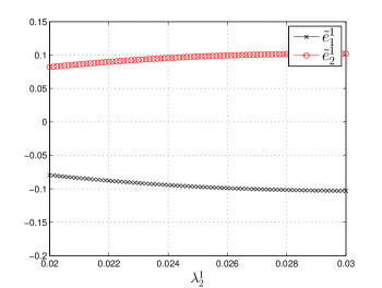
Figure 10: Steady-state perturbations in RFM $\#1$ in the RFMNP in Example 7 when changing $\lambda^{1}_{1}=1$ to $\bar{\lambda}^{1}_{1}=10$ for various values of $\lambda_{2}^{1}$.

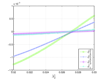
Figure 11: Steady-state perturbations in RFM $\#2$ in the RFMNP in Example 7 when changing $\lambda^{1}_{1}=1$ to $\bar{\lambda}^{1}_{1}=10$ for various values of $\lambda_{2}^{1}$.

Theorem 3 implies that when the codons of a gene are modified into “faster codons” (either via synthetic engineering or during evolution) then either all the translation rates of the other genes increase, or they all decrease. However, Theorem 3 does not provide information on when each of these two cases happens. In order to address this, we need to calculate derivatives of the equilibrium point coordinates with respect to the rates. The next result shows that these derivatives are well-defined. Denote the mapping from the parameters to the unique equilibrium point in $\operatorname{Int}(\Omega)$ by $\alpha$, that is, $e^{i}_{j}=\alpha^{i}_{j}(\lambda,H(0))$, $i=1,\dots,m$, $j=1,\dots,n_{i}$.

Proposition 4

The derivative $\frac{\partial}{\partial\lambda^{p}_{q}}\alpha^{i}_{j}(\lambda,H(0))$ exists for all $i,j,p,q$.

The next example uses these derivatives to obtain information on the two cases that can take place as we change one of the rates.

Example 8

Consider an RFMNP with $m=2$ RFMIO’s with lengths $n$ and $\ell$. To simplify the notation, let $e=\begin{bmatrix}e_{1},\dots,e_{n}\end{bmatrix}^{\prime}$ [$v=\begin{bmatrix}v_{1},\dots,e_{\ell}\end{bmatrix}^{\prime}$] denote the equilibrium point of RFMIO $\#1$ [RFMIO $\#2$], and let $\lambda_{i}$, $i=0,\dots,n$, denote the rates along RFMIO $\#1$. Suppose that $\lambda_{1}$ is changed to $\bar{\lambda}_{1}$. Differentiating the steady-state equations

$$\lambda_{0}G_{1}(e_{z})(1-e_{1})=\lambda_{1}e_{1}(1-e_{2}) =...=\lambda_{n-1}e_{n-1}(1-e_{n})=\lambda_{n}e_{n},$$

$$\sum_{i=1}^{n}e_{i}+\sum_{j=1}^{\ell}v_{j}+e_{z} =H(0),$$

w.r.t. $\lambda_{1}$ yields

$$\lambda_{0}G_{1}^{\prime}(e_{z})e_{z}^{\prime}(1-e_{1})-\lambda_{0}G_{1}(e_{z})e_{1}^{\prime} =\lambda_{n}e_{n}^{\prime},$$

$$e_{z}^{\prime}+\sum_{j=1}^{\ell}v_{j}^{\prime} =-\sum_{i=1}^{n}e_{i}^{\prime},$$

where we use the notation $f^{\prime}:=\frac{\partial}{\partial\lambda_{1}}f$. These two equations yield

$$(\lambda_{n}+\lambda_{0}G_{1}^{\prime}(e_{z})(1-e_{1}))e_{z}^{\prime}+\lambda_{n}\sum_{j=1}^{\ell}v_{j}^{\prime} =(\lambda_{0}G_{1}(e_{z})-\lambda_{n})e_{1}^{\prime}-\lambda_{n}\sum_{i=2}^{n-1}e_{i}^{\prime}.$$

Recall that $G_{1}(e_{z})>0$, $G_{1}^{\prime}(e_{z})>0$, $\lambda_{j}>0$ for all $j$, and $0<e_{p}<1$ for all $p$. Also, by Theorem 3, $e_{1}^{\prime}<0$, $e_{j}^{\prime}>0$, for all $j\in{2,...,n}$, and $\operatorname{{\mathrm{s}ign}}(e_{z}^{\prime})=\operatorname{{\mathrm{s}ign}}(v_{k}^{\prime})$, for all $k$. Thus,

$$\operatorname{{\mathrm{s}ign}}(e_{z}^{\prime})=\operatorname{{\mathrm{s}ign}}(v_{j}^{\prime}) =\operatorname{{\mathrm{s}ign}}\left((\lambda_{0}G_{1}(e_{z})-\lambda_{n})e_{1}^{\prime}-\lambda_{n}\sum_{i=2}^{n-1}e_{i}^{\prime}\right).$$ (22)

This means that the sign of the change in the densities in all the other RFMIO’s and the pool depends on several steady-state quantities including terms related to the initiation rate $\lambda_{0}G_{1}(e_{z})$ and exit rate $\lambda_{n}$ in RFMIO $\#1$, and also the change in the total density $\sum_{i=1}^{n-1}e_{i}^{\prime}$ in this RFMIO.

In the particular case $n=2$ (i.e., a very short RFM), Eq. (22) becomes:

$$\operatorname{{\mathrm{s}ign}}(e_{z}^{\prime})=\operatorname{{\mathrm{s}ign}}(v_{j}^{\prime}) =\operatorname{{\mathrm{s}ign}}(\lambda_{2}-\lambda_{0}G_{1}(e_{z})).$$ (23)

Note that $\lambda_{0}G_{1}(e_{z})$ [$\lambda_{2}$] is the steady-state initiation [exit] rate in RFMIO $\#1$. Thus, $\lambda_{2}-\lambda_{0}G_{1}(e_{z})>0$ means that it is “easier” for ribosomes to exit than to enter RFMIO $\#1$, and in this case (23) means that when $\lambda_{1}$ is increased the change in all other densities will be positive. This is intuitive, as more ribosomes will exit the modified molecule and this will improve the production rates in the other molecules. On the other-hand, if $\lambda_{2}-\lambda_{0}G_{1}(e_{z})<0$ then it is “easier” for ribosomes to enter than to exit RFMIO $\#1$, so increasing $\lambda_{1}$ will lead to an increased number of ribosomes in RFMIO $\#1$ and, by competition, to a decrease in the production rate in all the other RFMIOs. $\square$

Note that in the example above increasing $\lambda_{1}$ always increases the steady-state production rate $R=\lambda_{2}e_{2}$ in RFM $\#1$ (recall that $e_{2}^{\prime}>0$). One may expect that this will always lead to an increase in the production rate in the second RFMIO as well. However, the behavior in the RFMNP is more complicated because the shared pool generates a feedback connection between the RFMIO’s in the network. In particular, the effect on the other RFMIO’s depends not only on the modified production rate of RFMIO $\#1$, but on other factors including the change in the total ribosome density in RFMIO $\#1$ (see (22)).

This analysis of a very short RFM suggests that the steady-state initiation rate of the mRNA with the modified codon plays an important role in determining the effect of modifications in the network. If this initiation rate is relatively low (so it becomes the rate limiting factor), as believed to be the case in most endogenous genes [28], then the increase in the rate of one codon of the mRNA increases the translation rate in all the other mRNAs, whereas when this initiation rate is high then the opposite effect is obtained. This latter case may occur for example when a heterologous gene is highly expressed and thus “consumes” some of the available elongation/termination factors making the elongation rates the rate limiting factors.

IV Discussion

We introduced a new model, the RFMNP, for large-scale simultaneous translation and competition for ribosomes that combines several RFMIOs interconnected via a dynamic pool of free ribosomes. To the best of our knowledge, this is the first model of a network composed of interconnected RFMIOs. The RFMNP is amenable to analysis because it is a monotone dynamical system that admits a non-trivial first integral. Our results show that the RFMNP has several nice properties: it is an irreducible cooperative dynamical system admitting a continuum of linearly ordered equilibrium points, and every trajectory converges to an equilibrium point. The RFMNP is also on the “verge of contraction” with respect to the $\ell_{1}$ norm, and it entrains to periodic transition rates with a common period. The fact that the total number of ribosomes in the network is conserved means that local properties of any mRNA molecule (e.g., the abundance of the corresponding tRNA molecules) affects its own translation rate, and via competition, also globally affects the translation rates of all the other mRNAs in the network.

An important implication of our analysis and simulation results is that there are regimes and parameter values where there is a strong coupling between the different “translation components” (ribosomes and mRNAs) in the cell. Such regimes cannot be studied using models for translation of a single isolated mRNA molecule. The RFMNP is specifically important when studying highly expressed genes with many mRNA molecules and ribosomes translating them because the dynamics of such genes strongly affects the ribosomal pool. For example, changes in the translation dynamics of a heterologous gene which is expressed with a very strong promoter, resulting in very high mRNA copy number should affect the entire tRNA pool, and thus the translation of other endogenous genes. Highly expressed endogenous genes ”consume” many ribosomes. Thus, a mutation that affects their (“local”) translation rate is expected to affect also the translation dynamics of other mRNA molecules. Studying the evolution of such genes should be based on understanding the global effect of such mutations using a computational model such as the RFMNP.

On the other hand, we can approximate the dynamics of genes that are not highly expressed (e.g., a gene with mRNA levels that are $0.01\%$ of the mRNA levels in the cell) using a single RFM. In this case, the relative effect of the mRNA on all other mRNAs is expected to be limited.

Our analysis shows that increasing the translation initiation rate of a heterologous gene will always have a negative effect on the translation rate of other genes (i.e. their translation rates decrease) and vice versa. The effect of increasing [decreasing] the translation rate of a codon of the heterologous gene on the translation rate of other genes is more complicated: while it always increases [decreases] the translation rate of the heterologous gene it may either increase or decrease the translation rate of all other genes. The specific outcome of such a manipulation can be studied using the RFMNP with the parameters based on the heterologous genes and the host genome.

Our analysis suggests that the effect of improving the transition rate of a codon in an mRNA molecule on the production rate of other genes and the pool of ribosomes depends on the initiation rate in the modified mRNA. When the initiation rate is very low the effect is expected to be positive (all other production rates increase). However, if the initiation rate is high the effect may be negative. This may partially explain the selection for slower codons in highly expressed genes that practically decrease the initiation rate [67, 63]. This relation may also suggest a new factor that contributes to the evolution of highly expressed genes towards higher elongation and termination rates (i.e., the tendency of highly expressed genes to include “fast” codons). Indeed, lower elongation rates (and thus a relatively high initiation rate) may decrease the production rates of other mRNAs that are needed for proper functioning of the organism.

The RFM, and thus also the model described here, do not capture certain aspects of mRNA translation. For example, eukaryotic ribosomes may translate mRNAs in multiple cycles before entering the free ribosomal pool [70, 43, 31]. This phenomenon may perhaps be modeled by adding positive feedback [43] in the RFMNP. In addition, different genes are transcribed at different rates, resulting in a different number of (identical) mRNA copies for different genes. This can be modeled using a set of identical RFMs for each gene. Such a model can help in understanding how changes in mRNA levels of one gene affect the translation rates of all the mRNAs. The analysis here suggests that modifying the mRNA levels of a gene will affect the translation rates of all other genes in the same way. These and other aspects of biological translation may be integrated in our model in future studies. Ref. [25] develops the notion of the realizable region for steady-state gene expression under resource limitations, and methods for mitigating the effects of ribosome competition. Another interesting research direction is studying these topics in the context of the RFMNP.

The results reported here can be studied experimentally by designing and expressing a library of heterologous genes [72, 5, 32]. The effect of the manipulation of a codon (i.e, increasing or decreasing its rate) of the heterologous gene on the ribosomal densities and translation rates of all the mRNAs (endogenous and heterologous) can be performed via ribosome profiling [27] in addition to measurements of mRNA levels, translation rates, and protein levels [56].

We believe that networks of interconnected RFMIOs may prove to be powerful modeling and analysis tools for other natural and artificial systems as well. These include communication networks, intracellular trafficking in the cell, coordination of large groups of organisms (e.g., ants), traffic control, and more.

Appendix: Proofs

Proof of Proposition 1. We require the following result on repelling boundaries and persistence.

Lemma 1

Consider a time-varying system

$$\dot{x}=f(t,x)$$ (24)

whose trajectories evolve on $\Omega:=I_{1}\times I_{2}\times\ldots\times I_{n}\subseteq\mathbb{R}^{n}_{+}$, where each $I_{j}$ is an interval of the form $[0,A]$, $A>0$, or $[0,\infty)$. Suppose that the time-dependent vector field $f=\begin{bmatrix}f_{1},\ldots,f_{n}\end{bmatrix}^{\prime}$ has the following two properties:

• the cyclic boundary-repelling property (CBR): For each $\delta>0$ and each sufficiently small $\Delta>0$, there exists $K=K(\delta,\Delta)>0$ such that, for each $k=1,\ldots,n$ and each $t\geq 0$, the condition

  $$x_{k}(t)\leq\Delta,\text{ and }x_{k-1}(t)\geq\delta$$ (25)

  (all indexes are modulo $n$) implies that

  $$f_{k}(t,x)\geq K;$$ (26)

• for any $i\in\{1,\dots,n\}$, and any $s\geq 0$, $x_{i}(s)>0$ implies that

  $$x_{i}(t)>0,\quad\text{for all }t\geq s.$$ (27)

Then given any $\tau>0$ there exists $\varepsilon=\varepsilon(\tau)>0$, with $\varepsilon(\tau)\to 0$ as $\tau\to 0$, such that every solution $x(t,a)$, with $a\not=0$, satisfies

$$x_{i}(t,a)\geq\varepsilon\text{ for all }i\in\{1,\ldots,n\}\text{ and all }t\geq\tau.$$

In other words, the conclusion is that after an arbitrarily short time every $x_{i}(t,a)$ is separated away from zero.

Proof of Lemma 1. Pick $\tau>0$ and $a\not=0$. Then there exists $i\in\{1,\dots,n\}$ such that $a_{i}>0$. Since the (CBR) condition is cyclic, we may assume without loss of generality that $x_{n}(0)>0$. Then (27) implies that there exists $\delta>0$ such that $x_{n}(t)\geq\delta$ for all $t\in[0,\tau/n]$.

Fix $\Delta>0$ such that (CBR) holds. Let $K=K(\delta,\Delta)$, and define $\varepsilon_{1}:=\min\{\Delta,K\tau/n\}$. Let $t_{0}\in[0,\tau/n]$ be such that $x_{1}(t_{0})\geq\varepsilon_{1}$. Such a $t_{0}$ exists, since by property (CBR), $x_{1}(t)<\varepsilon_{1}\leq\Delta$ for all $t\in[0,\tau/n]$ would imply that $\dot{x}_{1}(t)=f_{1}(t,x(t))\geq K>0$ for all $t\in[0,\tau/n]$, which in turn implies $x_{1}(\tau/n)\geq x_{1}(0)+K\tau/n\geq K\tau/n\geq\varepsilon_{1}$, contradicting $x_{1}(\tau/n)<\varepsilon_{1}$. We claim that also $x_{1}(t)\geq\varepsilon_{1}$ for every $t\geq t_{0}$. Indeed, suppose otherwise. Then, there is some $t_{1}>t_{0}$ such that $\xi:=x_{1}(t_{1})<\varepsilon_{1}$. Let

$$\sigma:=\min\{t\geq t_{0}\,|\,x_{1}(t)\leq\xi\}>t_{0}.$$

As $x_{1}(\sigma)\leq\xi<\varepsilon_{1}\leq\Delta$, and $x_{n}(\sigma)>0$ property (CBR) says that $\dot{x}_{1}(\sigma)=f_{1}(\sigma,x(\sigma))>0$, so it follows that $\dot{x}_{1}(t)>0$ on an interval $[\sigma-c,\sigma]$, for some $c>0$. But then $x_{1}(\sigma-c)<x_{1}(\sigma)\leq\xi$, which contradicts the minimality of $\sigma$. Thus $x_{1}(t)\geq\varepsilon_{1}$ for all $t\geq t_{0}$, and in particular

$$x_{1}(t)\geq\varepsilon_{1},\quad\text{for all }t\geq\tau/n.$$ (28)

Let $\bar{K}:=K(\varepsilon_{1},\Delta)$, and define $\varepsilon_{2}:=\min\{\Delta,\bar{K}\tau/n\}$. Let $t_{0}\in[\tau/n,2\tau/n]$ be such that $x_{2}(t_{0})\geq\varepsilon_{2}$. Such a $t_{0}$ exists, since by property (CBR) and (28), $x_{2}(t)<\varepsilon_{2}\leq\Delta$ for all $t\in[\tau/n,2\tau/n]$ would imply that $\dot{x}_{2}(t)=f_{2}(t,x(t))\geq\bar{K}>0$ for all $t\in[\tau/n,2\tau/n]$, which in turn implies $x_{2}(2\tau/n)\geq x_{2}(\tau/n)+\bar{K}\tau/n\geq\bar{K}\tau/n\geq\varepsilon_{2}$, contradicting $x_{2}(2\tau/n)<\varepsilon_{2}$. We claim that also $x_{2}(t)\geq\varepsilon_{2}$ for every $t\geq t_{0}$. Indeed, suppose otherwise. Then, there is some $t_{1}>t_{0}$ such that $\xi:=x_{2}(t_{1})<\varepsilon_{2}$. Let

$$\sigma:=\min\{t\geq t_{0}\,|\,x_{2}(t)\leq\xi\}>t_{0}.$$

As $x_{2}(\sigma)\leq\xi<\varepsilon_{2}\leq\Delta$, and $x_{1}(\sigma)\geq\varepsilon_{1}$ property (CBR) says that $\dot{x}_{2}(\sigma)=f_{2}(\sigma,x(\sigma))>0$, so it follows that $\dot{x}_{2}(t)>0$ on an interval $[\sigma-c,\sigma]$, for some $c>0$. But then $x_{2}(\sigma-c)<x_{2}(\sigma)\leq\xi$, which contradicts the minimality of $\sigma$. Thus $x_{2}(t)\geq\varepsilon_{2}$ for all $t\geq t_{0}$, and in particular

$$x_{2}(t)\geq\varepsilon_{2},\quad\text{for all }t\geq 2\tau/n.$$

Continuing in this manner we have that for every $i\in\{1,\dots,n\}$ there exists $\varepsilon_{i}>0$ such that

$$x_{i}(t)\geq\varepsilon_{i},\quad\text{for all }t\geq i\tau/n.$$

Thus,

$$x_{i}(t)\geq\min\{\varepsilon_{1},\dots,\varepsilon_{n}\},\quad\text{for all }t\geq\tau\text{ and all }i=1,\dots,n,$$

and this completes the proof of Lemma 1. $\square$

We can now prove Proposition 1. Consider the case $m=1$, i.e. the RFMNP is given by

$$\dot{x}_{1} =\lambda_{0}(1-x_{1})G(x_{n+1})-\lambda_{1}x_{1}(1-x_{2}),$$

$$\dot{x}_{2} =\lambda_{1}x_{1}(1-x_{2})-\lambda_{2}x_{2}(1-x_{3}),$$

$$\vdots$$

$$\dot{x}_{n-1} =\lambda_{n-2}x_{n-2}(1-x_{n-1})-\lambda_{n-1}x_{n-1}(1-x_{n}),$$

$$\dot{x}_{n} =\lambda_{n-1}x_{n-1}(1-x_{n})-\lambda_{n}x_{n},$$

$$\dot{x}_{n+1} =\lambda_{n}x_{n}-\lambda_{0}(1-x_{1})G(x_{n+1}),$$ (29)

where we write $x_{n+1}$ instead of $z$. The proof in the case where $m>1$ is similar. We begin by showing that (Appendix: Proofs) satisfies the properties in Lemma 1 on $\Omega=[0,1]^{n}\times[0,\infty)$. Fix an arbitrary $\delta>0$. If $x_{1}\leq\Delta$ and $x_{n+1}\geq\delta$ then

$$f_{1} =\lambda_{0}(1-x_{1})G(x_{n+1})-\lambda_{1}x_{1}(1-x_{2})$$

$$\geq K_{1},$$

where $K_{1}:=\lambda_{0}(1-\Delta)G(\delta)-\lambda_{1}\Delta$. Now pick $1<k<n$. If $x_{k}\leq\Delta$ and $x_{k-1}\geq\delta$ then

$$f_{k} =\lambda_{k-1}x_{k-1}(1-x_{k})-\lambda_{k}x_{k}(1-x_{k+1})$$

$$\geq{K}_{k},$$

where

$${K}_{k}:=\lambda_{k-1}\delta(1-\Delta)-\lambda_{k}\Delta.$$

If $x_{n}\leq\Delta$ and $x_{n-1}\geq\delta$ for $1\leq i\leq n-1$ then

$$f_{n} =\lambda_{n-1}x_{n-1}(1-x_{n})-\lambda_{n}x_{n}$$

$$\geq{K_{n-1}}.$$

Finally, if $x_{n+1}\leq\Delta$ and $x_{n}\geq\delta$ then

$$f_{n+1} =\lambda_{n}x_{n}-\lambda_{0}(1-x_{1})G(x_{n+1})$$

$$\geq{K_{n+1}},$$

where $K_{n+1}:=\lambda_{n}\delta-\lambda_{0}G(\Delta)$. Thus, (26) holds for $K:=\min\{K_{1},\dots,K_{n+1}\}$, and clearly $K>0$ for all $\Delta>0$ sufficiency small. Thus, (Appendix: Proofs) satisfies (CBR).

To show that (Appendix: Proofs) also satisfies (27), note that for all $k\in\{1,\dots,n\}$ and all $x\in\Omega$, $\dot{x}_{k}\geq-\lambda_{k}x_{k}$, and that by the properties of $G(\cdot)$, $\dot{x}_{n+1}\geq-sx_{n+1}$ for all $x_{n+1}>0$ sufficiently small. Thus, (Appendix: Proofs) satisfies all the conditions in Lemma 1 and this implies that for any $\tau>0$ there exists $\varepsilon=\varepsilon(\tau/2)>0$ such that

$$x_{i}(t,a)\geq\varepsilon,\quad\text{for all }i\in\{1,\dots,n+1\}\text{ and all }t\geq\tau/2.$$ (30)

This proves the first part of Proposition 1. To complete the proof, define

$$y_{i}(t):=1-x_{n+1-i}(t),\quad i=1,\ldots,n,$$ (31)

and $y_{n+1}(t):=x_{n+1}(t)$. Then

$$\dot{y}_{1} =\lambda_{n}(1-y_{1})-\lambda_{n-1}y_{1}(1-y_{2}),$$

$$\dot{y}_{2} =\lambda_{n-1}y_{1}(1-y_{2})-\lambda_{n-2}y_{2}(1-y_{3}),$$

$$\vdots$$

$$\dot{y}_{n-1} =\lambda_{2}y_{n-2}(1-y_{n-1})-\lambda_{1}y_{n-1}(1-y_{n}),$$

$$\dot{y}_{n} =\lambda_{1}y_{n-1}(1-y_{n})-\lambda_{0}G(y_{n+1})y_{n},$$

$$\dot{y}_{n+1} =\lambda_{n}(1-y_{1})-\lambda_{0}G(y_{n+1})y_{n}.$$

The first $n$ equations here are an RFM with a time-varying exit rate $\lambda_{0}G(y_{n+1}(t))$. We already know that $y_{n+1}(t)\geq\varepsilon$ for all $t\geq\tau/2$ and the results in [39] imply that there exists $\varepsilon_{1}=\varepsilon_{1}(\tau)>0$ such that

$$y_{i}(t,a)\geq\varepsilon_{1},\quad\text{for all }i\in\{1,\dots,n\}\text{ and all }t\geq\tau.$$

Combining this with (31) completes the proof of Prop. 1. $\square$

Proof of Proposition 2. The Jacobian matrix $J$ of the RFMNP has the form

$$J=\begin{bmatrix}J_{1,1}&0&...&0&J_{1,{m+1}}\\ 0&J_{2,2}&...&0&J_{2,{m+1}}\\ \vdots&\vdots&...&\vdots\\ 0&0&...&J_{m,m}&J_{m,{m+1}}\\ J_{{m+1},1}&J_{{m+1},2}&...&J_{{m+1},m}&J_{{m+1},{m+1}}\end{bmatrix}\in\mathbb{R}^{d\times d}.$$ (32)

Here $J_{i,i}\in\mathbb{R}^{n_{i}\times n_{i}}$, $i=1,\dots,m$, is the Jacobian of RFMIO $\#i$ given by

$$\begin{bmatrix}-\lambda^{i}_{0}G_{i}(z)-\lambda^{i}_{1}(1-x^{i}_{2})&\lambda^{i}_{1}x^{i}_{1}&0&&0&0\\ \lambda^{i}_{1}(1-x^{i}_{2})&-\lambda^{i}_{1}x^{i}_{1}-\lambda^{i}_{2}(1-x^{i}_{3})&\lambda^{i}_{2}x^{i}_{2}&&0&0\\ 0&\lambda^{i}_{2}(1-x^{i}_{3})&-\lambda^{i}_{2}x^{i}_{2}-\lambda^{i}_{3}(1-x^{i}_{4})&&0&0\\ &&\vdots\\ 0&0&0&&-\lambda^{i}_{n_{i}-2}x^{i}_{n_{i}-2}-\lambda^{i}_{n_{i}-1}(1-x^{i}_{n_{i}})&\lambda^{i}_{n_{i}-1}x^{i}_{n_{i}-1}\\ 0&0&0&&\lambda^{i}_{n_{i}-1}(1-x^{i}_{n_{i}})&-\lambda^{i}_{{n_{i}}-1}x^{i}_{{n_{i}}-1}-\lambda^{i}_{n_{i}}\end{bmatrix},$$

and the other blocks are

$$J_{{m+1},i} =[\lambda^{i}_{0}G_{i}(z)\ 0\ ...\ 0\ \lambda^{i}_{n_{i}}]\in\mathbb{R}^{1\times n_{i}},$$

$$J_{i,{m+1}} =[\lambda^{i}_{0}(1-x_{1}^{i})G_{i}^{\prime}(z)\ 0\ ...\ 0]^{\prime}\in\mathbb{R}^{n_{i}\times 1},$$

$i=1,\dots,m$, and

$$J_{{m+1},{m+1}}=-\sum_{j=1}^{m}\lambda^{j}_{0}(1-x_{1}^{j})G_{j}^{\prime}(z)\in\mathbb{R}.$$

Since $x_{i}\in[0,1]$ and $\lambda^{i}_{j}>0$, every off-diagonal entry of $J_{i,i}$ is non-negative. Since $z\geq 0$, every entry of $J_{{m+1},j},J_{i,{m+1}}$, $i=1,\dots,m$, is also nonnegative. We conclude that every non-diagonal entry of $J$ is non-negative, and this implies (11) (see [59]). To prove (12), note that for any point in $\operatorname{Int}(\Omega)$ (i.e., $x_{j}\in(0,1)$, $j=1,\dots,d-1$, and $z>0$) every entry on the super- and sub-diagonal of $J_{i,i}$ is strictly positive. Also, $G_{i}(z)>0$, $i=1,\dots,m$. This implies that the matrix $J$ in (32) is irreducible. Combining this with Prop. 1 completes the proof. $\square$

Proof of Theorem 1. Since the RFMNP is a cooperative irreducible system on $\operatorname{Int}(\Omega)$ with a non-trivial first integral, Thm. 1 follows from combining Prop. 1 with the results in [46] (see also [51], [45] and [33] for related ideas). $\square$

Proof of Proposition 3. Recall that the matrix measure $\mu_{1}(\cdot):\mathbb{R}^{n\times n}\to\mathbb{R}$ induced by the $\ell_{1}$ norm is

$$\mu_{1}(A)=\max\{c_{1}(A),\dots,c_{n}(A)\},$$

where $c_{i}(A):=a_{ii}+\sum_{k\not=i}|a_{ki}|$, i.e. the sum of entries in column $i$ of $A$, with the off-diagonal entries taken with absolute value [68]. For the Jacobian of the RFMNP (32), we have $c_{i}(J(x))=0$ for all $i$ and all $x\in\Omega$, so $\mu_{1}(J(x))=0$. Now (16) follows from standard results in contraction theory (see, e.g., [54]). $\square$

Proof of Theorem 2. Write the PRFMNP as $\dot{x}=f(t,x)$. Then $f(t,y)=f(t+T,y)$ for all $t$ and $y$. Furthermore, $H$ in (9) is a non trivial first integral of the dynamics. Now Theorem 2 follows from the results in [61] (see also [30]). The fact that $\phi_{s}\in\operatorname{Int}(\Omega)$ follows from Proposition 1. $\square$

Proof of Theorem 3. To simplify the presentation, we prove the theorem for the case $m=2$ and change some of the notation. The proof in the general case is very similar. Let $n$ [$\ell$] denote the dimension of the first [second] RFMIO, and let $\lambda_{i}$ [$\zeta_{i}$] denote the rates in the first [second] RFMIO. We denote the state-variables of RFMIO $\#1$ by $x_{i}$, $i=1,\dots,n$, and those of the second RFMIO by $y_{i}$, $i=1,\dots,\ell$. Let $e_{i}$, $i=1,\dots,n$, [$v_{j}$, $j=1,\dots,\ell$] denote the equilibrium point of the first [second] RFMIO. Then we need to prove that

$$\tilde{e}_{i}<0,\text{ and }\tilde{e}_{j}>0,\text{ for all }j\in\{i+1,...,n\},$$ (33)

$$\operatorname{{\mathrm{s}ign}}(\tilde{v}_{1})=\dots=\operatorname{{\mathrm{s}ign}}(\tilde{v}_{\ell})=\operatorname{{\mathrm{s}ign}}(\tilde{e}_{z}),$$ (34)

where $\tilde{v}_{j}:=\bar{v}_{j}-v_{j}$. At steady state, the RFMNP equations yield:

$$\lambda_{0}G_{1}(e_{z})(1-e_{1}) =\lambda_{1}e_{1}(1-e_{2}),$$

$$=\lambda_{2}e_{2}(1-e_{3}),$$

$$=\lambda_{3}e_{3}(1-e_{4}),$$

$$\vdots$$

$$=\lambda_{n-1}e_{n-1}(1-e_{n})$$

$$=\lambda_{n}e_{n},$$ (35)

$$\zeta_{0}G_{2}(e_{z})(1-v_{1}) =\zeta_{1}v_{1}(1-v_{2}),$$

$$=\zeta_{2}v_{2}(1-v_{3}),$$

$$=\zeta_{3}v_{3}(1-v_{4}),$$

$$\vdots$$

$$=\zeta_{\ell-1}v_{\ell-1}(1-v_{\ell})$$

$$=\zeta_{\ell}v_{\ell},$$ (36)

$$\lambda_{n}e_{n}+\zeta_{\ell}v_{\ell} =\lambda_{0}G_{1}(e_{z})(1-e_{1})+\zeta_{0}G_{2}(e_{z})(1-v_{1}).$$ (37)

Also, since $H$ is a first integral

$$\sum_{i=1}^{n}e_{i}+\sum_{j=1}^{\ell}v_{j}+e_{z}=H(0).$$ (38)

Pick $i\in\{1,\dots,n-1\}$. Consider a new RFMNP obtained by modifying $\lambda_{i}$ in RFMIO $\#1$ to $\bar{\lambda}_{i}$, with $\bar{\lambda}_{i}>\lambda_{i}$. Then the equations for the modified equilibrium point are:

$$\lambda_{0}G_{1}(\bar{e}_{z})(1-\bar{e}_{1}) =\lambda_{1}\bar{e}_{1}(1-\bar{e}_{2}),$$

$$=\lambda_{2}\bar{e}_{2}(1-\bar{e}_{3}),$$

$$\vdots$$

$$=\bar{\lambda}_{i}\bar{e}_{i}(1-\bar{e}_{i+1}),$$

$$\vdots$$

$$=\lambda_{n-1}\bar{e}_{n-1}(1-\bar{e}_{n})$$

$$=\lambda_{n}\bar{e}_{n},$$ (39)

$$\zeta_{0}G_{2}(\bar{e}_{z})(1-\bar{v}_{1}) =\zeta_{1}\bar{v}_{1}(1-\bar{v}_{2}),$$

$$=\zeta_{2}\bar{v}_{2}(1-\bar{v}_{3}),$$

$$\vdots$$

$$=\zeta_{\ell-1}\bar{v}_{\ell-1}(1-\bar{v}_{\ell})$$

$$=\zeta_{\ell}\bar{v}_{\ell},$$ (40)

$$\lambda_{n}\bar{e}_{n}+\zeta_{\ell}\bar{v}_{\ell} =\lambda_{0}G_{1}(\bar{e}_{z})(1-\bar{e}_{1})+\zeta_{0}G_{2}(\bar{e}_{z})(1-\bar{v}_{1}).$$ (41)

Since the initial condition remains the same,

$$\sum_{i=1}^{n}e_{i}+\sum_{j=1}^{\ell}v_{j}+e_{z}=\sum_{i=1}^{n}\bar{e}_{i}+\sum_{j=1}^{\ell}\bar{v}_{j}+\bar{e}_{z}=H(0),$$

so

$$\sum_{i=1}^{n}\tilde{e}_{i}+\sum_{j=1}^{\ell}\tilde{v}_{j}+\tilde{e}_{z}=0.$$ (42)

The last equality in (36) yields

$$\zeta_{\ell-1}v_{\ell-1}=\frac{\zeta_{\ell}v_{\ell}}{1-v_{\ell}}.\\$$

The right-hand side here is increasing in $v_{\ell}$, and the left-hand side is increasing in $v_{\ell-1}$ (recall that $\zeta_{\ell}$ and $\zeta_{\ell-1}$ are the same for both the original and the modified RFMNP), so a change in $\lambda_{i}$ must lead to $\operatorname{{\mathrm{s}ign}}(\tilde{v}_{\ell-1})=\operatorname{{\mathrm{s}ign}}(\tilde{v}_{\ell})$. Using (36) again yields

$$\zeta_{\ell-2}v_{\ell-2}=\frac{\zeta_{\ell}v_{\ell}}{1-v_{\ell-1}},$$

so $\operatorname{{\mathrm{s}ign}}(\tilde{v}_{\ell-2})=\operatorname{{\mathrm{s}ign}}(\tilde{v}_{\ell-1})=\operatorname{{\mathrm{s}ign}}(\tilde{v}_{\ell})$. Continuing in this way yields

$$\operatorname{{\mathrm{s}ign}}(\tilde{v}_{1})=\operatorname{{\mathrm{s}ign}}(\tilde{v}_{2})=\dots=\operatorname{{\mathrm{s}ign}}(\tilde{v}_{\ell}).$$ (43)

By (36),

$$G_{2}(e_{z})=\frac{\zeta_{\ell}v_{\ell}}{\zeta_{0}(1-v_{1})}.$$

Since $G_{i}(p)$ is strictly increasing in $p$, combining this with (43) implies that $\operatorname{{\mathrm{s}ign}}(\tilde{e}_{z})=\operatorname{{\mathrm{s}ign}}(\tilde{v}_{1})=\operatorname{{\mathrm{s}ign}}(\tilde{v}_{2})=\dots=\operatorname{{\mathrm{s}ign}}(\tilde{v}_{\ell})$. This proves (34). To prove (33), note that arguing as above using (39) yields

$$\operatorname{{\mathrm{s}ign}}(\tilde{e}_{n})=\operatorname{{\mathrm{s}ign}}(\tilde{e}_{n-1})=\dots=\operatorname{{\mathrm{s}ign}}(\tilde{e}_{i+1}).$$

Seeking a contradiction, assume that $\operatorname{{\mathrm{s}ign}}(\tilde{e}_{i})=\operatorname{{\mathrm{s}ign}}(\tilde{e}_{n})$. By (39),

$$e_{i-1}=\frac{\lambda_{n}e_{n}}{\lambda_{i-1}(1-e_{i})}$$

so $\operatorname{{\mathrm{s}ign}}(\tilde{e}_{i-1})=\operatorname{{\mathrm{s}ign}}(\tilde{e}_{n})$, and continuing in this fashion yields

$$\operatorname{{\mathrm{s}ign}}(\tilde{e}_{n})=\operatorname{{\mathrm{s}ign}}(\tilde{e}_{n-1})=\dots=\operatorname{{\mathrm{s}ign}}(\tilde{e}_{1}).$$ (44)

By (35),

$$G_{1}(e_{z})=\frac{\lambda_{n}e_{n}}{\lambda_{0}(1-e_{1})},$$

and combining this with (44) implies that $\operatorname{{\mathrm{s}ign}}(\tilde{e}_{1})=...=\operatorname{{\mathrm{s}ign}}(\tilde{e}_{n})=\operatorname{{\mathrm{s}ign}}(\tilde{e}_{z})$. Since also $\operatorname{{\mathrm{s}ign}}(\tilde{v}_{1})=...=\operatorname{{\mathrm{s}ign}}(\tilde{v}_{\ell})=\operatorname{{\mathrm{s}ign}}(\tilde{e}_{z})$, it follows that all the differences have the same sign, and this contradicts (42). We conclude that if $\tilde{e}_{i}\not=0$ then $\operatorname{{\mathrm{s}ign}}(\tilde{e}_{i})\not=\operatorname{{\mathrm{s}ign}}(\tilde{e}_{i+1})=\operatorname{{\mathrm{s}ign}}(\tilde{e}_{i+2})=\dots=\operatorname{{\mathrm{s}ign}}(\tilde{e}_{n})$. To complete the proof of (33), we need to show that $\tilde{e}_{i}<0$. Seeking a contradiction, assume that $\tilde{e}_{i}\geq 0$, so $\tilde{e}_{i+1}\leq 0,\dots,\tilde{e_{n}}\leq 0$. Thus,

$$\bar{e}_{i}\geq e_{i},\quad\bar{e}_{i+1}\leq e_{i+1},\dots,\bar{e}_{n}\leq e_{n}.$$

By (35), $\lambda_{i}=\frac{\lambda_{n}e_{n}}{e_{i}(1-e_{i+1})}$, so

$$\frac{\bar{\lambda}_{i}-\lambda_{i}}{\lambda_{n}} =\frac{\bar{e}_{n}}{\bar{e}_{i}(1-\bar{e}_{i+1})}-\frac{e_{n}}{e_{i}(1-e_{i+1})}$$

$$\leq 0.$$

This contradiction completes the proof for the case where $i\in\{1,\dots,n-1\}$. The proof for the case $i=0$ and $i=n$ is similar. $\square$

Proof of Proposition 4. In [45], Mierczynski considered an irreducible cooperative dynamical system, $\dot{x}=f(x)$, that admits a non trivial first integral $H(x)$ with a positive gradient. Let $S_{x}:=\{v\in\mathbb{R}^{n}:\nabla H^{T}(x)v=0\}$, and consider the extended system

$$\dot{x} =f(x),$$

$$\dot{\delta x} =J(x)\delta x,$$

where $J:=\frac{\partial}{\partial x}f$ is the Jacobian, with initial condition $x(0)=x_{0}$, $\delta x(0)=\delta x_{0}\in S_{x}\setminus\{0\}$ . Mierczynski shows that there exists a norm, that depends on $x$, such that

$$|\delta x(t)|_{x(t)}<|\delta x_{0}|_{x_{0}},\quad\text{for all }t>0.$$

(For a general treatment on using Lyapunov-Finsler functions in contraction theory, see [18].) At the unique equilibrium point $e$ this yields

$$|\exp(J(e)t)\delta x_{0}|_{e}<|\delta x_{0}|_{e},\quad\text{for all }t>0.$$

This implies that the matrix obtained by restricting $J(e)$ to the integral manifold is Hurwitz and thus nonsingular. Invoking the implicit function theorem implies that the mapping from $\lambda$ to $e$ can be identified with a $C^{1}$ function. $\square$

References

- [1] D. Adams, B. Schmittmann, and R. Zia, “Far-from-equilibrium transport with constrained resources,” J. Stat. Mech., p. P06009, 2008.
- [2] U. Ala, F. A. Karreth, C. Bosia, A. Pagnani, R. Taulli, V. Leopold, Y. Tay, P. Provero, R. Zecchina, and P. P. Pandolfi, “Integrated transcriptional and competitive endogenous RNA networks are cross-regulated in permissive molecular environments,” Proceedings of the National Academy of Sciences, vol. 110, no. 18, pp. 7154–9, 2013.
- [3] Z. Aminzare and E. D. Sontag, “Contraction methods for nonlinear systems: A brief introduction and some open problems,” in Proc. 53rd IEEE Conf. on Decision and Control, Los Angeles, CA, 2014, pp. 3835–3847.
- [4] D. Angeli and E. D. Sontag, “Monotone control systems,” IEEE Trans. Automat. Control, vol. 48, pp. 1684–1698, 2003.
- [5] T. Ben-Yehezkel, S. Atar, H. Zur, A. Diament, E. Goz, T. Marx, R. Cohen, A. Dana, A. Feldman, E. Shapiro, and T. Tuller, “Rationally designed, heterologous S. cerevisiae transcripts expose novel expression determinants,” RNA Biol., 2015.
- [6] R. A. Blythe and M. R. Evans, “Nonequilibrium steady states of matrix-product form: a solver’s guide,” J. Phys. A: Math. Theor., vol. 40, no. 46, pp. R333–R441, 2007.
- [7] C. A. Brackley, M. C. Romano, and M. Thiel, “The dynamics of supply and demand in mRNA translation,” PLoS Comput. Biol., vol. 7, no. 10, p. e1002203, 10 2011.
- [8] H. Bremer and P. P. Dennis, Modulation of chemical composition and other parameters of the cell by growth rate, 2nd ed. Escherichia coli and Salmonella typhimurium: Cellular and Molecular Biology, 1996, ch. 97, p. 1559.
- [9] R. C. Brewster, F. M. Weinert, H. G. Garcia, D. Song, M. Rydenfelt, and R. Phillips, “The transcription factor titration effect dictates level of gene expression,” Cell, vol. 156, no. 6, pp. 1312–1323, 2014.
- [10] L. Carmel and E. Koonin, “A universal nonmonotonic relationship between gene compactness and expression levels in multicellular eukaryotes,” Genome Biol Evol., vol. 1, pp. 382–90, 2009.
- [11] C. Castillo-Davis, S. Mekhedov, D. Hartl, E. Koonin, and F. Kondrashov, “Selection for short introns in highly expressed genes.” Nat Genet., vol. 31, no. 4, pp. 415–8, 2002.
- [12] L. J. Cook and R. K. P. Zia, “Feedback and fluctuations in a totally asymmetric simple exclusion process with finite resources,” J. Stat. Mech., p. P02012, 2009.
- [13] L. J. Cook and R. K. P. Zia, “Competition for finite resources,” J. Stat. Mech., p. P05008, 2012.
- [14] A. Dana and T. Tuller, “Efficient manipulations of synonymous mutations for controlling translation rate–an analytical approach.” J. Comput. Biol., vol. 19, pp. 200–231, 2012.
- [15] A. Dana and T. Tuller, “The effect of trna levels on decoding times of mrna codons,” Nucleic Acids Res., vol. 42, no. 14, pp. 9171–81, 2014.
- [16] D. Del Vecchio and R. M. Murray, Biomolecular Feedback Systems. Princeton University Press, 2014.
- [17] E. Eisenberg and E. Levanon, “Human housekeeping genes are compact,” Trends Genet., vol. 19, no. 7, pp. 362–5, 2003.
- [18] F. Forni and R. Sepulchre, “A differential Lyapunov framework for contraction analysis,” IEEE Trans. Automat. Control, vol. 59, no. 3, pp. 614–628, 2014.
- [19] M. Frenkel-Morgenstern, T. Danon, T. Christian, T. Igarashi, L. Cohen, Y. M. Hou, and L. J. Jensen, “Genes adopt non-optimal codon usage to generate cell cycle-dependent oscillations in protein levels,” Mol. Syst. Biol., vol. 8, p. 572, 2012.
- [20] T. Galla, “Optimizing evacuation flow in a two-channel exclusion process,” J. Stat. Mech., p. P09004, 2011.
- [21] P. Greulich, L. Ciandrini, R. J. Allen, and M. C. Romano, “Mixed population of competing totally asymmetric simple exclusion processes with a shared reservoir of particles,” Phys. Rev. E, vol. 85, p. 011142, 2012.
- [22] A. Gyorgy and D. Del Vecchio, “Limitations and trade-offs in gene expression due to competition for shared cellular resources,” in Proc. 53rd IEEE Conf. on Decision and Control, Dec. 2014, pp. 5431–5436.
- [23] A. Gyorgy, J. I. Jimenez, J. Yazbek, H. Huang, H. Chung, R. Weiss, and D. Del Vecchio, “Isocost lines describe the cellular economy of genetic circuits,” Biophysical J., 2015, To appear.
- [24] M. Ha and M. den Nijs, “Macroscopic car condensation in a parking garage,” Phys. Rev. E, vol. 66, p. 036118, 2002.
- [25] A. Hamadeh and D. Del Vecchio, “Mitigation of resource competition in synthetic genetic circuits through feedback regulation,” in Proc. 53rd IEEE Conf. on Decision and Control, Dec. 2014, pp. 3829–3834.
- [26] Q. Hui and W. M. Haddad, “Distributed nonlinear control algorithms for network consensus,” Automatica, vol. 44, no. 9, pp. 2375–2381, 2008.
- [27] N. T. Ingolia, S. Ghaemmaghami, J. R. Newman, and J. S. Weissman, “Genome-wide analysis in vivo of translation with nucleotide resolution using ribosome profiling,” Science, vol. 324, no. 5924, pp. 218–23, 2009.
- [28] N. Jacques and M. Dreyfus, “Translation initiation in Escherichia coli: old and new questions,” Mol Microbiol., vol. 4, no. 7, pp. 1063–7, 1990.
- [29] M. Jens and N. Rajewsky, “Competition between target sites of regulators shapes post-transcriptional gene regulation,” Nat Rev Genet., vol. 16, no. 2, pp. 113–26, 2015.
- [30] J. Ji-Fa, “Periodic monotone systems with an invariant function,” SIAM J. Math. Anal., vol. 27, pp. 1738–1744, 1996.
- [31] G. Kopeina, Z. A. Afonina, K. Gromova, V. Shirokov, V. Vasiliev, and A. Spirin, “Step-wise formation of eukaryotic double-row polyribosomes and circular translation of polysomal mRNA,” Nucleic Acids Res., vol. 36, no. 8, pp. 2476–2488, 2008.
- [32] G. Kudla, A. W. Murray, D. Tollervey, and J. B. Plotkin, “Coding-sequence determinants of gene expression in Escherichia coli,” Science, vol. 324, pp. 255–258, 2009.
- [33] P. D. Leenheer, D. Angeli, and E. D. Sontag, “Monotone chemical reaction networks,” J. Mathematical Chemistry, vol. 41, pp. 295–314, 2007.
- [34] G.-W. Li, E. Oh, and J. Weissman, “The anti-Shine-Dalgarno sequence drives translational pausing and codon choice in bacteria,” Nature, vol. 484, no. 7395, pp. 538–41, 2012.
- [35] S. Li, L. Feng, and D. Niu, “Selection for the miniaturization of highly expressed genes,” Biochem Biophys Res Commun., vol. 360, no. 3, pp. 586–92, 2007.
- [36] W. Lohmiller and J.-J. E. Slotine, “On contraction analysis for non-linear systems,” Automatica, vol. 34, pp. 683–696, 1998.
- [37] J. Lu and C. Deutsch, “Electrostatics in the ribosomal tunnel modulate chain elongation rates,” J. Mol. Biol., vol. 384, p. 73ָ6, 2008.
- [38] C. T. MacDonald, J. H. Gibbs, and A. C. Pipkin, “Kinetics of biopolymerization on nucleic acid templates,” Biopolymers, vol. 6, pp. 1–25, 1968.
- [39] M. Margaliot, E. D. Sontag, and T. Tuller, “Entrainment to periodic initiation and transition rates in a computational model for gene translation,” PLoS ONE, vol. 9, no. 5, p. e96039, 2014.
- [40] M. Margaliot, E. Sontag, and T. Tuller, “Contraction after small transients,” Submitted. [Online]. Available: arXiv:1506.06613
- [41] M. Margaliot and T. Tuller, “On the steady-state distribution in the homogeneous ribosome flow model,” IEEE/ACM Trans. Computational Biology and Bioinformatics, vol. 9, pp. 1724–1736, 2012.
- [42] M. Margaliot and T. Tuller, “Stability analysis of the ribosome flow model,” IEEE/ACM Trans. Computational Biology and Bioinformatics, vol. 9, pp. 1545–1552, 2012.
- [43] Margaliot, M. and Tuller, T., “Ribosome flow model with positive feedback,” J. Royal Society Interface, vol. 10, p. 20130267, 2013.
- [44] W. Mather, J. Hasty, L. Tsimring, and R. Williams, “Translational cross talk in gene networks,” Biophys J., vol. 104, no. 11, pp. 2564–72, 2013.
- [45] J. Mierczynski, “A class of strongly cooperative systems without compactness,” Colloq. Math., vol. 62, pp. 43–47, 1991.
- [46] J. Mierczynski, “Cooperative irreducible systems of ordinary differential equations with first integral,” ArXiv e-prints, 2012. [Online]. Available: http://arxiv.org/abs/1208.4697
- [47] S. Pechmann and J. Frydman, “Evolutionary conservation of codon optimality reveals hidden signatures of cotranslational folding,” Nat Struct Mol Biol., vol. 20, no. 2, pp. 237–43, 2013.
- [48] G. Poker, Y. Zarai, M. Margaliot, and T. Tuller, “Maximizing protein translation rate in the nonhomogeneous ribosome flow model: a convex optimization approach,” J. Royal Society Interface, vol. 11, no. 100, 2014.
- [49] G. Poker, M. Margaliot, and T. Tuller, “Sensitivity of mRNA translation,” Sci. Rep., vol. 5, p. 12795, 2015.
- [50] Y. Qian and D. Del Vecchio, “Effective interaction graphs arising from resource limitations in gene networks,” in Proc. American Control Conference (ACC2015), Chicago, IL, 2015.
- [51] A. Raveh, Y. Zarai, M. Margaliot, and T. Tuller, “Ribosome flow model on a ring,” IEEE/ACM Trans. Computational Biology and Bioinformatics, 2015, To appear. [Online]. Available: http://ieeexplore.ieee.org/xpl/articleDetails.jsp?arnumber=7078877
- [52] S. Reuveni, I. Meilijson, M. Kupiec, E. Ruppin, and T. Tuller, “Genome-scale analysis of translation elongation with a ribosome flow model,” PLOS Computational Biology, vol. 7, p. e1002127, 2011.
- [53] J. D. Richter and L. D. Smith, “Differential capacity for translation and lack of competition between mRNAs that segregate to free and membrane-bound polysomes,” Cell, vol. 27, pp. 183–191, 1981.
- [54] G. Russo, M. di Bernardo, and E. D. Sontag, “Global entrainment of transcriptional systems to periodic inputs,” PLOS Computational Biology, vol. 6, p. e1000739, 2010.
- [55] R. Sabi and T. Tuller, “A comparative genomics study on the effect of individual amino acids on ribosome stalling,” BMC genomics, 2015.
- [56] B. Schwanhausser, D. Busse, N. Li, G. Dittmar, J. Schuchhardt, J. Wolf, W. Chen, and M. Selbach, “Global quantification of mammalian gene expression control,” Nature, vol. 473, no. 7347, pp. 337–42, 2011.
- [57] P. M. Sharp, L. R. Emery, and K. Zeng, “Forces that influence the evolution of codon bias,” Philos. Trans. R. Soc. Lond. B, vol. 365, no. 1544, pp. 1203–12, 2010.
- [58] L. B. Shaw, R. K. P. Zia, and K. H. Lee, “Totally asymmetric exclusion process with extended objects: a model for protein synthesis,” Phys. Rev. E, vol. 68, p. 021910, 2003.
- [59] H. L. Smith, Monotone Dynamical Systems: An Introduction to the Theory of Competitive and Cooperative Systems, ser. Mathematical Surveys and Monographs. Providence, RI: Amer. Math. Soc., 1995, vol. 41.
- [60] P. Spellman, G. Sherlock, M. Zhang, V. Iyer, K. Anders, M. Eisen, P. Brown, D. Botstein, and B. Futcher, “Comprehensive identification of cell cycle-regulated genes of the yeast Saccharomyces cerevisiae by microarray hybridization,” Mol Biol Cell., vol. 9, no. 12, pp. 3273–97, 1998.
- [61] B. Tang, Y. Kuang, and H. Smith, “Strictly nonautonomous cooperative system with a first integral,” SIAM J. Math. Anal., vol. 24, pp. 1331–1339, 1993.
- [62] G. Tripathy and M. Barma, “Driven lattice gases with quenched disorder: exact results and different macroscopic regimes,” Phys. Rev. E, vol. 58, pp. 1911–1926, 1998.
- [63] T. Tuller, A. Carmi, K. Vestsigian, S. Navon, Y. Dorfan, J. Zaborske, T. Pan, O. Dahan, I. Furman, and Y. Pilpel, “An evolutionarily conserved mechanism for controlling the efficiency of protein translation,” Cell, vol. 141, no. 2, pp. 344–54, 2010.
- [64] T. Tuller, E. Ruppin, and M. Kupiec, “Properties of untranslated regions of the S. cerevisiae genome,” BMC Genomics, vol. 10, p. 329, 2009.
- [65] T. Tuller, I. Veksler, N. Gazit, M. Kupiec, E. Ruppin, and M. Ziv, “Composite effects of the coding sequences determinants on the speed and density of ribosomes,” Genome Biol., vol. 12, no. 11, p. R110, 2011.
- [66] T. Tuller, Y. Y. Waldman, M. Kupiec, and E. Ruppin, “Translation efficiency is determined by both codon bias and folding energy,” Proceedings of the National Academy of Sciences, vol. 107, no. 8, pp. 3645–50, 2010.
- [67] T. Tuller and H. Zur, “Multiple roles of the coding sequence 5’ end in gene expression regulation,” Nucleic Acids Res., vol. 43, no. 1, pp. 13–28, 2015.
- [68] M. Vidyasagar, Nonlinear Systems Analysis. Englewood Cliffs, NJ: Prentice Hall, 1978.
- [69] J. Vind, M. A. Sorensen, M. D. Rasmussen, and S. Pedersen, “Synthesis of proteins in Escherichia coli is limited by the concentration of free ribosomes: expression from reporter genes does not always reflect functional mRNA levels,” J. Mol. Biol., vol. 231, pp. 678–88, 1993.
- [70] T. von der Haar, “Mathematical and computational modelling of ribosomal movement and protein synthesis: an overview,” Computational and Structural Biotechnology J., vol. 1, no. 1, pp. 1–7, 2012.
- [71] J. Warner, “The economics of ribosome biosynthesis in yeast,” Trends Biochem Sci., vol. 24, no. 11, pp. 437–40, 1999.
- [72] M. Welch, S. Govindarajan, J. E. Ness, A. Villalobos, A. Gurney, J. Minshull, and C. Gustafsson, “Design parameters to control synthetic gene expression in Escherichia coli,” PLoS One, vol. 4, no. 9, p. e7002, 2009.
- [73] Y. Zarai, M. Margaliot, and T. Tuller, “Maximizing protein translation rate in the ribosome flow model: the homogeneous case,” IEEE/ACM Trans. Computational Biology and Bioinformatics, vol. 11, pp. 1184–1195, 2014.
- [74] D. Zenklusen, D. R. Larson, and R. H. Singer, “Single-RNA counting reveals alternative modes of gene expression in yeast,” Nat. Struct. Mol. Biol., vol. 15, pp. 1263–1271, 2008.