Conserved Charge Susceptibilities in a Chemically Frozen Hadronic Gas

Abstract

In a hadronic gas with three conserved charges (electric charge, baryon number, and strangeness) we employ the hadron resonance gas model to compute both diagonal and off-diagonal susceptibilities. We model the effect of chemical freeze-out in two ways: one in which all particle numbers are conserved below the chemical freeze-out temperature and one which takes into account resonance decays. We then briefly discuss possible implications these results may have on two active areas of research, hydrodynamic fluctuations and the search for the QCD critical point.

I Introduction

Analysis of fluctuations has been of great interest to the heavy ion collision physics community in recent years. One line of research examines the impact of pre-equilibrium initial state fluctuations on observed final state momentum anisotropies (see Gale:2013da for a review). In addition to initial state effects, fluctuations of a thermal nature will occur after the system formed in a heavy ion collision has attained local equilibrium. The enhancement of such fluctuations is an expected experimental signature of the QCD critical point Stephanov:1998dy ; Stephanov:1999zu ; Hatta:2003wn . The principle goal of the Beam Energy Scan at RHIC is the discovery of the QCD critical point, and the STAR collaboration has recently reported results in this direction Adamczyk:2013dal .

Thermal fluctuations can also lead to observable particle correlations Kapusta:2011gt ; Springer:2012iz ; Ling:2013ksb . These correlations can be extended over a large pseudorapidity range because they are sourced by fluctuations which propagate or diffuse according to the equations of hydrodynamics. Such correlations are experimentally studied by measuring balance functions Abelev:2013csa ; Aggarwal:2010ya .

To examine the effect of (thermal) conserved charge fluctuations over the history of a heavy-ion collision, one needs thermodynamical input, as the magnitude of such fluctuations are controlled by the susceptibilities

$$\chi_{\alpha\beta}\equiv{\frac{\partial^{2}P}{\partial\mu_{\alpha}\partial\mu_{\beta}}}$$ (1)

where $P$ is the pressure, $\mu$ denotes chemical potential, and the abstract indices $\alpha$, $\beta$ denote the particular conserved charge under consideration. In this work, $\alpha$ can take on the value $Q,B,S$ for electric charge, baryon number, or strangeness. (In fact, as explained in Ling:2013ksb , the relevant quantity is actually $\chi_{\alpha\beta}T/s$ where $s$ is the entropy density.) One obvious source of input on these thermodynamic quantities is lattice QCD, as the susceptibilities have been calculated there Borsanyi:2010cj ; Borsanyi:2011sw ; Bazavov:2012jq . However, as the lattice assumes full thermal and chemical equilibrium, its results may not accurately reflect the thermodynamics in a heavy ion collision where chemical equilibrium is not always maintained. It is the effect of chemical freeze-out on the conserved charge susceptibilities which we wish to explore in this work. For the highest energy collisions at RHIC and LHC, the net charge, baryon number, and strangeness of the fireball are approximately zero. Hence, for the remainder of this paper we calculate susceptibilities at $\mu_{B}=\mu_{Q}=\mu_{S}=0$.

The effect of chemical freeze-out on thermodynamics in heavy ion collisions has a long history going back more than two decades Bebie:1991ij ; Hirano:2002ds ; Teaney:2002aj ; Huovinen:2007xh ; Huovinen:2009yb . However, these discussions have exclusively focused on pressure $P$ and energy density $\varepsilon$, with emphasis the equation of state $P(\varepsilon)$ as this is necessary input for hydrodynamic simulations. It was found that despite the fact that both $P(T)$ and $\varepsilon(T)$ are both modified after including the effects of chemical freeze-out, $P(\varepsilon)$ is affected only slightly Teaney:2002aj .

Given the recent interest in fluctuations we thus wish to reopen the line of inquiry with particular attention paid to the susceptibilities. To accomplish this, we employ the hadron resonance gas model (HRG) Dashen:1969ep ; Venugopalan:1992hy ; Becattini:2004td which (in full equilibrium) has proved to be an excellent approximation to lattice calculations at low temperatures ($T\lesssim 180$ MeV). By including the effects of chemical non-equilibration in the HRG, we expect the results to more accurately represent the thermodynamics of the system formed in a heavy ion collision.

The following is the outline of the paper. In Sec. II, we review the thermodynamics of the HRG model. We then proceed to detail two ways of modeling chemical freeze-out. We refer to the first as “Full chemical Freeze Out” (FFO) and explain the details in Sec. III wherein all number changing processes cease below the freeze-out temperature $T<T_{\rm ch}$ and hence all particle numbers are constant. We also provide some new analytical formulas for the chemical potentials and susceptibilities. In Sec. IV, we detail the second model of chemical freeze-out referred to as Partial Chemical Equilibrium (PCE) Bebie:1991ij which permits resonances with short lifetimes to decay. We present the results for the susceptibilities in Sec. V. We comment on interesting features of the results, possible phenomenological implications and directions for future work in Sec. VI.

II Review of Hadron Resonance Gas Thermodynamics

At temperatures below the deconfinement temperature ($T\lesssim 180\,{\rm MeV}$), the thermalized matter left in the wake of a heavy ion collision can be modeled as a gas of non-interacting, point-like hadrons. The effect of interactions is incorporated by including resonances. This model is parameter-free, and does a remarkably good job of approximating lattice QCD data at sufficiently low temperatures Bazavov:2012jq .

II.1 Pressure, Entropy Density, Number Density

To access relevant thermodynamic quantities, one may start by considering the partial pressure of a given particle species (labeled with the subscript ‘i’). Assuming the momentum distribution is isotropic, the expression is

$$P_{i}(T,\mu_{i})=\frac{g_{i}}{6\pi^{2}}\int_{0}^{\infty}\frac{p^{4}}{E_{i}}\left[\frac{dp}{e^{(E_{i}-\mu_{i})/T}\pm 1}\right]$$ (2)

where the upper/lower signs refer to fermions/bosons, $E_{i}^{2}=p^{2}+m_{i}^{2}$ and $g_{i}$ is a spin degeneracy factor, We have included a chemical potential $\mu_{i}$ associated with this particular particle. It is more convenient to write $\mu_{i}$ in terms of chemical potentials associated with the conserved charges: baryon number (B), electric charge (Q), and strangeness (S) as we will see shortly.

The number density of this particle is found by

$$n_{i}(T,\mu_{i})={\left(\frac{\partial P}{\partial\mu_{i}}\right)_{T}}=\frac{g_{i}}{2\pi^{2}}\int_{0}^{\infty}\frac{p^{2}dp}{e^{(E_{i}-\mu_{i})/T}\pm 1}$$ (3)

The second equality is a more familiar expression for the number density, and can be found by first taking the derivative of (2) and then performing an integration by parts.

We will also need an expression for the partial entropy

$$s_{i}(T,\mu_{i}) = {\left(\frac{\partial P}{\partial T}\right)_{\mu_{i}}}$$

$$= \frac{g_{i}}{2\pi^{2}T}\int_{0}^{\infty}\left[E_{i}-\mu_{i}+\frac{p^{2}}{3E_{i}}\right]\frac{p^{2}dp}{e^{(E_{i}-\mu_{i})/T}\pm 1}$$

The second equality can be found by first taking the derivative of (2) and then performing integration by parts, or more directly by using the thermodynamic identity

$$Ts_{i}=\varepsilon_{i}+P_{i}-\mu_{i}n_{i}$$ (5)

where $\varepsilon_{i}$ is the energy density of the particle “i”. In order to compute the total entropy density $s$ and/or the total pressure $P$, one must sum over all hadronic species $i$,

$$P(T,\{\mu\})=\sum_{i}P_{i}(T,\mu_{i}).$$ (6)

Note that the total pressure is a function of the set of all chemical potentials, which we denote $\{\mu\}$. The HRG is parameter free, but one must choose which particles to include in a given calculation. We include particles and resonances listed by the particle data group (PDG) Agashe:2014kda with masses less than or equal to 2 GeV. More details on our included particles and their decays can be found in Appendix A.

II.2 Conserved Charges and Susceptibilities in Full Equilibrium (FE)

We are interested in fluctuations of conserved charges; as such it pays to work with chemical potentials associated with these conserved charges only. In later sections, when we consider chemical freeze-out, certain particle numbers are conserved and hence we will introduce additional conserved “charges” and chemical potentials.

The total density of charge $\alpha$ in the system is

$$n_{\alpha}(T,\{\mu\})=\sum_{i}\alpha_{i}n_{i}(T,\mu_{i})$$ (7)

where $\alpha_{i}$ is the conserved charge $\alpha$ of the $i$th particle. For example, the electric charge density can be found by setting the abstract index $\alpha=Q$:

$$n_{Q}(T,\{\mu\})=\sum_{i}Q_{i}n_{i}(T,\mu_{i})$$ (8)

Every conserved charge has a corresponding chemical potential, so by definition we could alternatively write

$$n_{\alpha}(T,\{\mu\})=\sum_{i}{\left(\frac{\partial P_{i}(T,\mu_{i})}{\partial\mu_{\alpha}}\right)_{T}}=\sum_{i}n_{i}(T,\mu_{i}){\left(\frac{\partial\mu_{i}}{\partial\mu_{\alpha}}\right)_{T}}.$$ (9)

Comparing (7) with (9) we see that

$$\alpha_{i}={\left(\frac{\partial\mu_{i}}{\partial\mu_{\alpha}}\right)_{T}}.$$ (10)

This can only be satisfied if the “particle” chemical potentials are related to the conserved charge chemical potentials as

$$\mu_{i}=\sum_{\alpha}\alpha_{i}\mu_{\alpha}$$ (11)

or, in less abstract notation,

$$\mu_{i}=Q_{i}\mu_{Q}+B_{i}\mu_{B}+S_{i}\mu_{S}$$ (12)

where $Q_{i},B_{i},S_{i}$ are the electric charge, baryon number, and strangeness of the $i$th particle.

We now consider the (3 $\times$ 3) matrix of susceptibilities

$$\chi_{\alpha\beta} = {\frac{\partial n_{\alpha}(T,\{\mu\})}{\partial\mu_{\beta}}}=\sum_{i}\alpha_{i}\beta_{i}{\frac{\partial n_{i}(T,\mu_{i})}{\partial\mu_{i}}}$$ (13)

In terms of thermodynamic integrals, the components of the susceptibility matrix are

$$\chi_{\alpha\beta}(T,\{\mu\})=\sum_{i}\frac{g_{i}\alpha_{i}\beta_{i}}{2\pi^{2}T}\int_{0}^{\infty}\frac{e^{(E_{i}-\mu_{i})/T}p^{2}dp}{\left[e^{(E_{i}-\mu_{i})/T}\pm 1\right]^{2}}$$ (14)

For example, the baryon-strangeness susceptibility is found by setting $\alpha=B$, $\beta=S$,

$$\chi_{\rm BS}(T,\{\mu\})=\sum_{i}\frac{g_{i}B_{i}S_{i}}{2\pi^{2}T}\int_{0}^{\infty}\frac{e^{(E_{i}-\mu_{i})/T}p^{2}dp}{\left[e^{(E_{i}-\mu_{i})/T}\pm 1\right]^{2}}$$ (15)

II.3 Boltzmann Approximation

If quantum statistics are necessary, one needs to use the expressions given in the previous subsection to compute relevant thermodynamic quantities. However, for physical hadronic masses and temperatures below deconfinement, quantum statistics represent only a small correction to the classical results. The classical expressions are advantageous due to their analytical tractability. We will exclusively use the Boltzmann approximation for the remainder of this work. For Boltzmann statistics, we can neglect the $\pm 1$ in the distribution function. The remaining integrals can be done analytically leading to

$$n_{i}(T,\mu_{i}) = n_{i}^{\rm FE}(T)e^{\mu_{i}/T}$$ (16)

$$s_{i}(T,\mu_{i}) = n_{i}(T,\mu_{i})\left[\frac{m_{i}}{T}\frac{K_{3}(m_{i}/T)}{K_{2}(m_{i}/T)}-\frac{\mu_{i}}{T}\right]$$ (17)

where $K_{2}(x)$ is a modified Bessel function. The function $n_{i}^{\rm FE}(T)$ is the number density in full equilibrium (FE), and where all chemical potentials vanish $\mu_{B}=\mu_{Q}=\mu_{S}=0$ (which is the case shortly after thermalization in a high energy heavy ion collision).

$$n_{i}^{\rm FE}(T) \equiv \frac{g_{i}T^{3}}{2\pi^{2}}\left(\frac{m_{i}}{T}\right)^{2}K_{2}\left(\frac{m_{i}}{T}\right)$$ (18)

The total entropy in full equilibrium (and where all chemical potentials vanish) is

$$s^{\rm FE}(T) = \sum_{i}n^{\rm FE}_{i}(T)\left[\frac{m_{i}}{T}\frac{K_{3}(m_{i}/T)}{K_{2}(m_{i}/T)}\right].$$ (19)

The susceptibilities are given by

$$\chi_{\alpha\beta}^{\rm FE}(T)=\frac{T^{2}}{2\pi^{2}}\sum_{i}\alpha_{i}\beta_{i}g_{i}\left(\frac{m_{i}}{T}\right)^{2}K_{2}\left(\frac{m_{i}}{T}\right)$$ (20)

Given a list of hadrons with masses $m_{i}$, the (full equilibrium) susceptibilities as a function of temperature can be calculated using (20). Calculations of this sort were carried out and compared with lattice QCD results in Bazavov:2012jq .

III Full chemical Freeze Out (FFO)

The results of the previous section are applicable for a system in full chemical equilibrium. The system created in a heavy ion collision is not static and has a finite size; it does not remain in chemical equilibrium throughout its entire evolution. Eventually, number changing processes freeze out, and the only remaining interactions between hadrons are elastic scattering processes. During this phase, the system is chemically frozen out (but still in local thermal equilibrium).

A first attempt to model this phase can be made by considering the total number of each species of hadron ($N_{i}\equiv n_{i}V$ where $V$ is the volume of the system) to be fixed Hirano:2002ds . We use the superscript “FFO” to denote “Full Freeze-Out”, meaning each hadron species has a fixed number after chemical freeze-out. In reality, some particles decay; we include this effect in the next section.

To maintain this chemical freeze-out condition, we must introduce additional chemical potentials corresponding to the new conserved particle numbers. Assuming each species of hadron is conserved after chemical freeze-out, there will be one new chemical potential for each hadron. Hence:

$$\mu_{i}=Q_{i}\mu_{Q}+B_{i}\mu_{B}+S_{i}\mu_{S}+\mu^{\rm FFO}_{\rm i}$$ (21)

The additional chemical potential $\mu^{\rm FFO}_{i}$ vanishes while the system is in chemical equilibrium, but becomes active after chemical freeze-out. One can think of this as suddenly associating a conserved “charge” with each species of hadron. For example, $\pi^{+}$ particles have a (+1) $\pi^{+}$ “charge”, $\pi^{0}$ particles have a (+1) $\pi^{0}$ “charge” (and zero $\pi^{+},\pi^{-}$ “charge”), etc…

In order to remove any dependence on the volume of the system, it is more convenient to impose the condition

$$\frac{n_{i}(T,\mu_{i}^{\rm FFO})}{s(T,\{\mu^{\rm FFO}\})}=\frac{n^{\rm FE}_{i}(T_{\rm ch})}{s^{\rm FE}(T_{\rm ch})}$$ (22)

where the right hand side is a constant. The temperature $T_{\rm ch}$ is the chemical freeze-out temperature below which number changing processes are no longer effective. This condition is equivalent to $N_{i}=\rm{constant}$ because (neglecting dissipative corrections) the total entropy $sV$ is also conserved.

III.1 Analytical Results

The central problem is how to determine the temperature dependence of all of the chemical potentials $\mu^{\rm FFO}_{i}$ such that condition (22) is satisfied. In this subsection, we give some analytical formulas for the chemical potentials and susceptibilities which (to the best of our knowledge) have not previously appeared in the literature.

Assuming $\mu_{B}=\mu_{Q}=\mu_{S}=0$ we have $\mu_{j}=\mu^{\rm FFO}_{j}$. If we have a system of $N_{\rm tot}$ species of particles, there are $N_{\rm tot}-1$ constraints of the form

$$\frac{n_{j}(T,\mu_{j}^{\rm FFO})}{n_{i}(T,\mu_{i}^{\rm FFO})}=\frac{n_{j}^{\rm FE}(T_{\rm ch})}{n_{i}^{\rm FE}(T_{\rm ch})}$$ (23)

Substituting (16) and (18), one can solve for the difference

$$\frac{\mu^{\rm FFO}_{j}(T)-\mu^{\rm FFO}_{i}(T)}{T}=\ln\left[\frac{K_{2}(m_{i}/T)K_{2}(m_{j}/T_{\rm ch})}{K_{2}(m_{i}/T_{\rm ch})K_{2}(m_{j}/T)}\right]$$ (24)

Note that at $T=T_{\rm ch}$, the difference vanishes implying all of the chemical potentials are the same at that point (of course, by definition they should all vanish at $T=T_{\rm ch}$ which we will show shortly).

The final constraint is found by summing (17) over all hadrons and dividing both sides by $s$, which leads to

$$1=\sum_{j}\frac{n_{j}(T,\mu_{j}^{\rm FFO})}{s(T,\{\mu^{\rm FFO}\})}\left[\frac{m_{j}}{T}\frac{K_{3}(m_{j}/T)}{K_{2}(m_{j}/T)}-\frac{\mu^{\rm FFO}_{j}}{T}\right]$$ (25)

Substituting (22), the expressions for $n_{j}$ and $s$ in full equilibrium (18),(19), and the constraint (24) one can solve analytically for $\mu_{i}^{\rm FFO}$

$$\frac{\mu_{i}^{\rm FFO}(T)}{T}=\ln\left[\frac{K_{2}(m_{i}/T_{\rm ch})}{K_{2}(m_{i}/T)}\right]-\Delta(T)$$ (26)

where $\Delta(T)$ is a temperature dependent offset which is independent of the mass $m_{i}$

$$\Delta(T)\equiv\frac{\sum_{j}g_{j}m_{j}^{2}K_{2}(m_{j}/T_{\rm ch})\left[G\left(\frac{m_{j}}{T}\right)-G\left(\frac{m_{j}}{T_{\rm ch}}\right)\right]}{\sum_{j}g_{j}m_{j}^{2}K_{2}(m_{j}/T_{\rm ch})}$$ (27)

and we have defined

$$G(x)\equiv\frac{xK_{3}(x)}{K_{2}(x)}+\ln\left[K_{2}(x)\right]$$ (28)

Plots of the chemical potentials as a function of $T$ are shown in Fig. 1 assuming $T_{\rm ch}=160$ MeV.

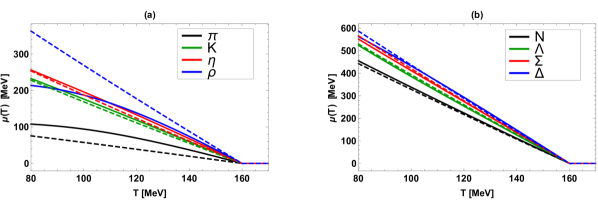
Figure 1: (Color Online) Results for the particle chemical potentials $\mu_{i}^{\rm FFO}$ and $\mu_{i}^{\rm PCE}$ which enforce the chemical freeze-out condition. Shown are the chemical potentials for the four lightest mesons (a) and the four lightest baryons (b). The dashed lines are the chemical potentials given the FFO freeze-out condition, the solid lines are the chemical potentials given the PCE freeze-out condition. We assumed $T_{\rm ch}=160$ MeV.

Once $T_{\rm ch}$ is specified, and a set of particles to include in the HRG is fixed, one can use (26) to determine the chemical potential for each species of particle as a function of $T$. When these are known, one can go back and compute the susceptibilities by inserting the correct $\mu^{\rm FFO}(T)$ for each species of particle,

$$\chi_{\alpha\beta}^{\rm FFO}(T)=\frac{1}{T}\sum_{i}\alpha_{i}\beta_{i}n_{i}(T,\mu_{i}^{\rm FFO}(T))$$ (29)

which can be written

$$\chi_{\alpha\beta}^{\rm FFO}(T)=\frac{T^{2}e^{-\Delta(T)}}{2\pi^{2}}\sum_{i}\alpha_{i}\beta_{i}g_{i}\left(\frac{m_{i}}{T}\right)^{2}K_{2}\left(\frac{m_{i}}{T_{\rm ch}}\right).$$ (30)

This analytical formula for susceptibility (and associated formulae for the chemical potentials) in “full freeze-out” is one of our main results.

III.2 Approximate Chemical Potentials for $m_{i}\gg T$

In our calculations, we use (26) to compute the chemical potentials in the case of full freeze-out. However, to develop our intuition, it is useful to consider an approximation which leads to simpler results. The HRG model should be applicable for temperatures of the order 100 MeV $\lesssim$ T $\lesssim$ 180 MeV, below deconfinement and above kinetic freeze-out. For these temperatures, most hadrons have $m\gg T$ except for the lowest mass ones (pions).

For $m\gg T$, one can use the asymptotic approximation for the modified Bessel functions

$$K_{n}(x)\approx\sqrt{\frac{\pi}{2x}}e^{-x}\left[1+\mathcal{O}\left(\frac{1}{x}\right)\right]$$ (31)

If we assume that $m_{i}\gg T_{\rm ch}>T$, and keep only the leading order in the asymptotic expansion, the chemical potentials are found to be approximately linear in $m$ with a temperature dependent offset

$$\mu^{\rm FFO}_{i}(T)\approx m_{i}\left[1-\frac{T}{T_{\rm ch}}\right]-T\left[\ln\left(\sqrt{\frac{T}{T_{\rm ch}}}\right)+\Delta(T)\right].$$ (32)

A similar approximation was used in previous calculations Teaney:2002aj . Unfortunately, a simple approximation for $\Delta$ is more difficult to come by since the sum over $j$ necessary to compute $\Delta$ runs over all hadrons, some of which have $m\sim T$.

Assuming a freeze-out temperature of $T_{\rm ch}=160$ MeV, for high mass particles ($m\sim 1$ GeV) and low temperatures ($T\sim 100$ MeV), the approximate formula differs from the analytic result by less than 3%.

In summary, for physical hadron masses and temperatures realized in a heavy ion collision, the “full freeze out” chemical potentials are approximately linear with temperature (plus corrections). Corrections to this approximation are due to both the contributions at $m\sim T$, and quantum statistics.

IV Including decays - Partial Chemical Equilibrium (PCE)

In reality, the number of each particle is not precisely conserved after chemical freeze-out due to the fact that resonances decay. For example, the number of $\rho$ mesons is not constant, since they will primarily decay into pions. In order to account for this, we use the model of partial chemical equilibrium detailed in Bebie:1991ij which we review here for completeness.

We consider only a subset of particles to be stable (i.e. those with lifetimes much longer than timescale of a heavy ion collision). We denote number of stable particles and the total number of particles as $N_{S}$, $N_{\rm tot}$ respectively. We follow Teaney:2002aj in choosing the stable hadrons to be $\pi,K,\eta,\omega,N,\eta^{\prime},\phi,\Lambda,\Sigma,\Xi,\Omega$ (we include all members of any isospin multiplet and all antibaryons). Each of these stable particles has an associated chemical potential $\bar{\mu}^{\rm PCE}_{i}$. The generalization of (12) is now

$$\mu^{\rm PCE}_{i}=Q_{i}\mu_{Q}+B_{i}\mu_{B}+S_{i}\mu_{S}+\sum_{j,\rm stable}d_{ij}\bar{\mu}_{j}^{\rm PCE}.$$ (33)

Note that the summation runs only over stable particles. The coefficients $d_{ij}$ are the “charges” associated with the stable conserved chemical potentials. For example, whereas in the full freeze-out case, a $\rho^{+}$ particle would have (+1) “$\rho^{+}$ charge”, in the PCE case a $\rho^{+}$ particle has (+1) “$\pi^{+}$ charge” and (+1) “$\pi^{0}$ charge” since a $\rho^{+}$ decays to $\pi^{+}\pi^{0}$ 100% of the time.

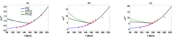
Figure 2: (color online) Dimensionless thermodynamic quantities pressure (a), energy density (b), and entropy density (c) in the case of full chemical equilibrium (FE), full freeze-out (FFO), and partial chemical equilibrium (PCE) assuming $T_{\rm ch}=160$ MeV. The red points are lattice data adapted from Borsanyi:2010cj

More generally, the $d_{ij}$ coefficients are found by examining the decay rates of particle $i$ which result in one (or more) stable particles $j$. Computation of the $d_{ij}$ requires branching ratios for each hadron and resonance included in the HRG. In Appendix A we provide more details on the determination of these decay rates, many of which are not measured precisely. The precise value $d_{ij}$ is found by multiplying the branching fraction for the decay by the number of stable particles $j$ formed in that decay, and finally summing over all decay modes of $i$. In other words, $d_{ij}$ is the average number of stable particles $j$ formed from a decay of particle $i$. A stable particle can be thought of one which decays into itself 100% of the time, so for example $d_{\pi^{0}i}=\delta_{\pi^{0}i}$.

It is helpful to envision a matrix, $\mathbf{d}$, which has $N$ rows, and $N_{S}$ columns. In appendix B we provide a portion of this matrix, (and hence give a subset of the $d_{ij}$ coefficients).

The quantity which is now conserved after chemical freeze-out is

$$\bar{N}_{i}=\sum_{j}N_{j}d_{ji}$$ (34)

which is the “effective number of stable particles”, including those hidden inside the unstable particles which will eventually decay. For example, if we had a system of only $\rho$ and $\pi$ particles, the number

$$\bar{N}_{\pi^{+}}=N_{\pi^{+}}+N_{\rho^{+}}$$ (35)

would be conserved after chemical freeze-out, since a $\rho^{+}$ effectively counts as one $\pi^{+}$. Similarly, the quantity

$$\bar{N}_{\pi^{0}}=N_{\pi^{0}}+N_{\rho^{+}}+N_{\rho^{-}}$$ (36)

is conserved since both $\rho^{+}$ and $\rho^{-}$ effectively count as one $\pi^{0}$.

As before, to remove any dependence on the volume of the system, the freeze-out condition is implemented using intensive quantities

$$\frac{\bar{n}_{i}(T,\{\bar{\mu}^{\rm PCE}\})}{s(T,\{\bar{\mu}^{\rm PCE}\})}=\frac{\bar{n}_{i}^{\rm FE}(T_{\rm ch})}{s^{\rm FE}(T_{\rm ch})}\equiv\bar{C}_{i}$$ (37)

This criteria is more complicated than the full freeze-out case, since $\bar{n}_{i}$ now depends on multiple chemical potentials. As before, we set up a system of $N_{S}$ algebraic equations for $\{\bar{\mu}^{\rm PCE}\}$. There are $N_{S}-1$ constraints which can be written without any reference to $s$:

$$\frac{\bar{n}_{i}(T,\{\bar{\mu}^{\rm PCE}\})}{n_{\Omega}(T,\bar{\mu}^{\rm PCE}_{\Omega})}=\frac{\bar{C}_{i}}{\bar{C}_{\Omega}}$$ (38)

It is advantageous to single out the heaviest stable particle ($\Omega$) because it is both stable ($d_{\Omega i}=\delta_{\Omega i}$), and none of the other particles we consider decay into it ($d_{i\Omega}=\delta_{i\Omega}$). Hence, $\bar{n}_{\Omega}(T,\{\bar{\mu}^{\rm PCE}\})=n_{\Omega}(T,\bar{\mu}^{\rm PCE}_{\Omega})$. To make the dependence on the chemical potentials explicit, we can re-write these equations as

$$\bar{C}_{i}n_{\Omega}^{\rm FE}(T)e^{\frac{\bar{\mu}_{\Omega}^{\rm PCE}}{T}}=\bar{C}_{\Omega}\sum_{j}n_{j}^{\rm FE}(T)d_{ji}\exp\left[\sum_{k}\frac{d_{jk}\bar{\mu}^{\rm PCE}_{k}}{T}\right]$$ (39)

One more equation is necessary to close the set. We take it to be

$$\bar{C}_{\Omega}\frac{s(T,\{\bar{\mu}^{\rm PCE}\})}{n_{\Omega}(T,\bar{\mu}_{\Omega}^{\rm PCE})}=1$$ (40)

Substituting (17), and making use of (38), we find

$$\sum_{i}\frac{s_{i}^{\rm FE}(T)}{n_{\Omega}^{\rm FE}(T)}\exp\left[\sum_{k}\frac{d_{ik}\bar{\mu}^{\rm PCE}_{k}}{T}\right]=e^{\frac{\bar{\mu}_{\Omega}^{\rm PCE}}{T}}\left[1+\sum_{i}\frac{\bar{C}_{i}\bar{\mu}_{i}^{\rm PCE}}{T}\right]$$ (41)

The right hand side of (41) makes use of the fact that

$$\sum_{i=1}^{N_{\rm tot}}\mu^{\rm PCE}_{i}n_{i}=\sum_{i,\rm stable}\bar{\mu}^{\rm PCE}_{i}\bar{n}_{i}.$$ (42)

The second sum runs only over the stable particles. This relation is straightforward to show given (33) and (34).

Eqs. (39) and (41) form a nonlinear system of $N_{S}$ algebraic equations for the set of chemical potentials $\{\bar{\mu}^{\rm PCE}\}$. Unlike the “Full Freeze-Out” case, we have been unable to solve this system analytically. The system can be solved numerically (for example) with a matrix formulation of Newton’s method, but in practice we find the most efficient way to solve the system is with Mathematica’s built-in FindRoot[] function MMA10 . Results for both light mesons and baryons are shown in Fig. 1

V Results and discussion

With the results for the chemical potentials of each particle in hand, we can then compute thermodynamic quantities of interest. The energy density, pressure and entropy density are shown in Fig. 2. We also include lattice data in our plots; we re-emphasize that the PCE and FFO results are not expected to agree with the lattice, since lattice calculations presuppose full chemical equilibrium.

The susceptibilities can be seen in Fig 3. Note that the inclusion of chemical freeze-out can have a large effect compared to a fully equilibrated system, especially at low temperatures where the full equilibrium susceptibilities are approximately vanishing. With regard to the inclusion of decays via PCE, we see that with only a few exceptions, the PCE scenario amounts to roughly an $\mathcal{O}$(10%) correction to the FFO scenario, as long as $T>100$ MeV.

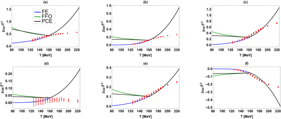
Figure 3: (color online) Dimensionless susceptibilities in the case of full chemical equilibrium (FE), full freeze-out (FFO), and partial chemical equilibrium (PCE) assuming $T_{\rm ch}=160$ MeV. The red points are lattice data adapted from Borsanyi:2011sw .

When considering the magnitude of hydrodynamic fluctuations, the quantity $\chi T/s$ is the relevant one Ling:2013ksb . We plot this combination in Fig. 4.

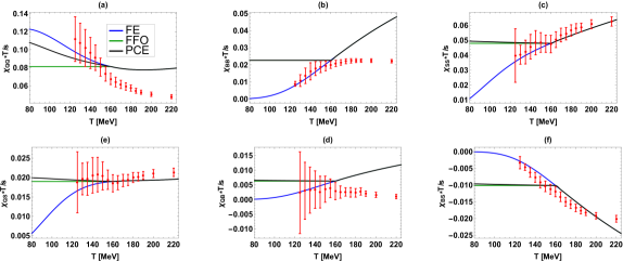
Figure 4: (color online) Susceptibility to entropy density ratio in the case of full chemical equilibrium (FE), full freeze-out (FFO), and partial chemical equilibrium (PCE) assuming $T_{\rm ch}=160$ MeV. The red points are lattice data adapted from Borsanyi:2011sw .

At temperatures below $T_{\rm ch}$, $\chi^{\rm FFO}_{\alpha\beta}T/s$ is exactly constant (since $\chi\sim\sum_{i}n_{i}$ and $n_{i}/s$ is constant). The inclusion of partial chemical equilibrium amounts to a very small correction in most cases.

The baryon-baryon susceptibility is especially interesting. In the case of $\chi_{BB}/s$, the PCE and FFO curves lie on top of each other, and (within our numerical precision) the numerical values are exactly the same. We suspect that $(\chi_{BB}/s)^{\rm CFO}=(\chi_{BB}/s)^{\rm PCE}$ but were unable to show this analytically. It is also interesting to note that if we switch from the HRG model to the lattice data at around 160 MeV, then $\chi_{BB}T/s$ is approximately constant throughout the entire range $80\,{\rm MeV}\leq T\leq 220$ MeV, which is simple to deal with analytically.

The BB susceptibility is also phenomenologically interesting, as it is important for net proton fluctuations which are used to search for the critical point. It is quite tempting to determine whether the inclusion of chemical freeze-out can improve the agreement of the HRG with the STAR measurements of these fluctuations Fukushima:2014lfa ; Albright:2015uua . Simple considerations show that for any additional chemical potentials to have an effect on the skewness or kurtosis, one must move beyond the Boltzmann approximation used in this paper. In our notation, the skewness measured in experiment is

$$S\sigma\equiv\frac{T}{\chi_{BB}}{\frac{\partial\chi_{BB}}{\partial\mu_{B}}}.$$ (43)

Using (29), and noting that all baryons have $B_{i}^{2}=1$,

$$\chi_{BB}T = \sum_{i}n_{i}(T,\mu_{i})$$ (44)

$${\frac{\partial\chi_{BB}}{\partial\mu_{B}}} = \frac{1}{T^{2}}\sum_{i}B_{i}n_{i}(T,\mu_{i})$$ (45)

Breaking the sum over $i$ into baryons and anti-baryons and noting the only difference in the two is the sign of $\mu_{B}$ and $B_{i}$, we have

$${\frac{\partial\chi_{BB}}{\partial\mu_{B}}} = \frac{2}{T^{2}}\sinh(\mu_{B}/T)\sum_{i,\rm baryons}n_{i}(T,\mu_{i})\Bigl{.}\Bigr{|}_{\mu_{B}=0}$$ (46)

$$\chi_{BB}T = 2\cosh(\mu_{B}/T)\sum_{\rm i,baryons}n_{i}(T,\mu_{i})\Bigl{.}\Bigr{|}_{\mu_{B}=0}.$$ (47)

And hence

$$S\sigma=\tanh(\mu_{B}/T)$$ (48)

which is independent of whether the system is in chemical equilibrium or frozen out. Similarly, the kurtosis $\kappa\sigma^{2}$ can be shown to be equal to 1 whether or not one employs chemical freeze-out. Thus, whether or not chemical freeze-out of hadrons can improve the agreement of the HRG with STAR measurements requires more careful consideration which is beyond the scope of this paper; we defer it to future work.

VI Conclusion

We have computed all six components of the susceptibility matrix for three conserved charges: electric charge, baryon number, and strangeness. We have done so using the hadron-resonance gas model employing two different implementations of chemical freeze-out.

In almost all cases, the inclusion of chemical freeze-out enhances $\chi_{\alpha\beta}T/s$ at low temperatures relative to the full equilibrium case. Thus we expect that the fluctuations at low temperatures will generally be larger than those found if one exclusively uses thermodynamic data from the lattice. This appears consistent with the findings of Albright:2015uua . The exception is the diagonal electric charge susceptibility $\chi_{QQ}T/s$ which is a decreasing function of $T$. Thus, the inclusion of chemical freeze-out will tend to reduce electric charge fluctuations relative to equilibrium.

With regard to correlations and balance functions measured in experiment Abelev:2013csa ; Aggarwal:2010ya : as compared to full equilibrium, the inclusion of chemical freeze-out will tend to narrow the pseudorapidity ($\Delta\eta$) width of the balance function (for a given diffusion constant). The reason is that enhanced fluctuations at late times (low temperatures) have less time to diffuse. The inclusion of resonance decays via PCE is unlikely to affect the balance functions except in the case of electric charge fluctuations. As seen in Fig. 4 (a), for $\chi_{QQ}T/s$, partial chemical equilibrium tends to significantly reduce the effect of chemical freeze-out, as the PCE curve lies closer to the full equilibrium curve than the one for full freeze-out.

In summary, the inclusion of chemical freeze-out is an important difference between the thermodynamics of a physical heavy ion collision and lattice QCD calculations. This effect has implications for (among other things) particle correlations and balance functions, and the search for the QCD critical point. Work to explore these implications is already underway.

Appendix A Particles, Resonances, and Decays

We include all hadrons and resonances listed in the 2014 PDG (with rating of *** or ****) with masses $\lesssim$ 2 GeV. The most massive particle we consider is the $f_{2}(2010)$, but we omit $f_{0}(600)$ ($\sigma$ meson) Broniowski:2015oha . The masses and quantum numbers of all included particles match those given in the 2014 Review of Particle Physics provided by the PDG Agashe:2014kda .

The measured decay modes and branching fractions of the higher mass resonances are very uncertain. Often decay channels are simply labeled as “seen” and/or the measured branching fractions do not sum to one. Hence, theoretical input is required. We rely almost exclusively on previous work by Josef Sollfrank and Pasi Huovinen who created a table of decays from the 2005 PDG data, supplemented by educated guesses based on the behavior of similar resonances and the fact that the branching ratios must sum to one Huovinen:PC ; PasiOnline .

We have not attempted to update all branching fractions to incorporate more recent PDG data, as our results are most sensitive to lower mass hadrons/resonances, which were already measured precisely in 2005. Nevertheless, we have added three new resonances which were not present in the 2005 Review of Particle Physics: $\pi_{2}(1880)$, $N(1875)$ and $N(1900)$. The branching ratios for each of these resonances are very poorly known, hence (as in the original table) we rely on theoretical input and educated guesses to estimate decay rates of these particles. These branching fractions do not significantly affect our results, but we include them here for completeness. Our assumptions are given in Table LABEL:BrTable, and we explain our rationale as follows.

For the $\pi_{2}(1880)$, no decay modes are listed in the PDG. Our assumed branching fractions rely on the nearby resonance $\pi_{2}(1670)$ and the results of the model of Li:2008xy . For the $N(1875)$, the PDG listings of the measured branching fractions do not sum to one. We attempt consistency with the measured values, forcing the sum to be one. For the $N(1900)$, the measured branching fractions sum to less than 50%. We assume that the remainder is in the form of decays to $N\rho$, as is the case for the nearby resonance $N(1720)$ (which has identical quantum numbers). Finally, for the $a_{4}(2040)$, the PDG lists only a few decay modes as “seen”. Our input for this resonance is almost entirely theoretical, we start from the calculations of Pang:2015eha and then include the $K\bar{K}$ and $\eta^{\prime}\pi$ modes to make the sum of the branching ratios one.

Table 1: Assumed branching fractions for newly discovered resonances

$\pi_{2}(1880)\longrightarrow\rho\pi$	(33%)
$\pi_{2}(1880)\longrightarrow f_{2}(1270)\pi$	(17%)
$\pi_{2}(1880)\longrightarrow\rho\omega$	(17%)
$\pi_{2}(1880)\longrightarrow KK^{*}$	(11%)
$\pi_{2}(1880)\longrightarrow\rho(1450)\pi*$	(11%)
$\pi_{2}(1880)\longrightarrow a(1320)\eta$	(11%)
$N(1875)\longrightarrow N\pi$	(10 %)
$N(1875)\longrightarrow N\omega$	(20 %)
$N(1875)\longrightarrow\Delta\pi$	(50 %)
$N(1875)\longrightarrow N\pi\pi$	(15 %)
$N(1875)\longrightarrow N\rho$	(5 %)
$N(1900)\longrightarrow N\pi$	(6 %)
$N(1900)\longrightarrow\rho\eta$	(12 %)
$N(1900)\longrightarrow\rho\omega$	(12 %)
$N(1900)\longrightarrow\Lambda K$	(4 %)
$N(1900)\longrightarrow\Sigma K$	(6 %)
$N(1900)\longrightarrow N\rho$	(60 %)
$a_{4}(2040)\longrightarrow\rho\omega$	(37%)
$a_{4}(2040)\longrightarrow\rho\pi$	(20 %)
$a_{4}(2040)\longrightarrow b_{2}(1235)\pi$	(22 %)
$a_{4}(2040)\longrightarrow f_{2}(1270)\pi$	(11 %)
$a_{4}(2040)\longrightarrow K\bar{K}$	(5 %)
$a_{4}(2040)\longrightarrow\eta^{\prime}\pi$	(5 %)

Appendix B Sample Decay Coefficients for Partial Chemical Equilibrium

As a convenience to the reader, Table LABEL:dijtable is a sample of the “effective number of stable particles” formed from each unstable particle (i.e. some of the $d_{ij}$ coefficients). Note that this is only a partial list.

While we have tabulated the $d_{ij}$ coefficients for photons produced in decays, we omit the photon when computing thermodynamic quantities like $n$, $s$ and $\chi_{\alpha\beta}$ as it is not expected that these photons will thermalize and they are not considered part of the HRG model.

Table 2: Incomplete list of the coefficients $d_{ij}$. The top row lists the 18 lightest stable particles. The first column lists the lightest 26 unstable particles. The table entry of the $ith$ row, $jth$ column is the coefficient $d_{ij}$. We omit columns for the heavier $\Sigma,\Xi,\Omega$ (their entries are all zero for the selection of unstable particles listed).

	$\gamma$	$\pi^{+}$	$\pi^{0}$	$\pi^{-}$	$K^{+}$	$K^{-}$	$K^{0}$	$\bar{K}^{0}$	$\eta$	$\omega$	$p$	$\bar{p}$	$n$	$\bar{n}$	$\eta^{\prime}$	$\phi$	$\Lambda$	$\bar{\Lambda}$
$\rho^{+}$	0	1.000	1.000	0	0	0	0	0	0	0	0	0	0	0	0	0	0	0
$\rho^{0}$	0	1.000	0	1.000	0	0	0	0	0	0	0	0	0	0	0	0	0	0
$\rho^{-}$	0	0	1.000	1.000	0	0	0	0	0	0	0	0	0	0	0	0	0	0
$K^{*}(892)^{+}$	0	0.667	0.333	0	0.333	0	0.667	0	0	0	0	0	0	0	0	0	0	0
$K^{*}(892)^{-}$	0	0	0.333	0.667	0	0.333	0	0.667	0	0	0	0	0	0	0	0	0	0
$K^{*}(892)^{0}$	0	0	0.333	0.667	0.667	0	0.333	0	0	0	0	0	0	0	0	0	0	0
$\bar{K}^{*}(892)^{0}$	0	0.667	0.333	0	0	0.667	0	0.333	0	0	0	0	0	0	0	0	0	0
$f_{0}(980)$	0	0.52	0.52	0.52	0.11	0.11	0.11	0.11	0	0	0	0	0	0	0	0	0	0
$a_{0}(980)^{+}$	0	0.844	0	0	0.156	0	0	0.156	0.844	0	0	0	0	0	0	0	0	0
$a_{0}(980)^{0}$	0	0	0.844	0	0.078	0.078	0.078	0.078	0.844	0	0	0	0	0	0	0	0	0
$a_{0}(980)^{-}$	0	0	0	0.844	0	0.156	0.156	0	0.844	0	0	0	0	0	0	0	0	0
$h_{1}(1170)$	0	1.000	1.000	1.000	0	0	0	0	0	0	0	0	0	0	0	0	0	0
$b_{1}(1235)^{+}$	0	1.000	0	0	0	0	0	0	0	1.000	0	0	0	0	0	0	0	0
$b_{1}(1235)^{0}$	0	0	1.000	0	0	0	0	0	0	1.000	0	0	0	0	0	0	0	0
$b_{1}(1235)^{-}$	0	0	0	1.000	0	0	0	0	0	1.000	0	0	0	0	0	0	0	0
$a_{1}(1260)^{+}$	0	1.000.5	1.000	0.5	0	0	0	0	0	0	0	0	0	0	0	0	0	0
$a_{1}(1260)^{0}$	0	1.000	1.000	1.000	0	0	0	0	0	0	0	0	0	0	0	0	0	0
$a_{1}(1260)^{-}$	0	0.5	1.000	1.5	0	0	0	0	0	0	0	0	0	0	0	0	0	0
$\Delta^{++}$	0	1.000	0	0	0	0	0	0	0	0	1.000	0	0	0	0	0	0	0
$\bar{\Delta}^{++}$	0	0	0	1.000	0	0	0	0	0	0	0	1.000	0	0	0	0	0	0
$\Delta^{+}$	0.006	0.331	0.663	0	0	0	0	0	0	0	0.669	0	0.331	0	0	0	0	0
$\bar{\Delta}^{+}$	0.006	0	0.663	0.331	0	0	0	0	0	0	0	0.669	0	0.331	0	0	0	0
$\Delta^{0}$	0.006	0	0.663	0.331	0	0	0	0	0	0	0.331	0	0.669	0	0	0	0	0
$\bar{\Delta}^{0}$	0.006	0.331	0.663	0	0	0	0	0	0	0	0	0.331	0	0.669	0	0	0	0
$\Delta^{-}$	0	0	0	1.000	0	0	0	0	0	0	0	0	1.000	0	0	0	0	0
$\bar{\Delta}^{-}$	0	1.000	0	0	0	0	0	0	0	0	0	0	0	1.000	0	0	0	0

References

- (1) C. Gale, S. Jeon, and B. Schenke, “Hydrodynamic Modeling of Heavy-Ion Collisions,” Int.J.Mod.Phys. A28 (2013) 1340011, arXiv:1301.5893 [nucl-th].
- (2) M. A. Stephanov, K. Rajagopal, and E. V. Shuryak, “Signatures of the tricritical point in QCD,” Phys. Rev. Lett. 81 (1998) 4816–4819, arXiv:hep-ph/9806219 [hep-ph].
- (3) M. A. Stephanov, K. Rajagopal, and E. V. Shuryak, “Event-by-event fluctuations in heavy ion collisions and the QCD critical point,” Phys. Rev. D60 (1999) 114028, arXiv:hep-ph/9903292 [hep-ph].
- (4) Y. Hatta and M. A. Stephanov, “Proton number fluctuation as a signal of the QCD critical endpoint,” Phys. Rev. Lett. 91 (2003) 102003, arXiv:hep-ph/0302002 [hep-ph]. [Erratum: Phys. Rev. Lett.91,129901(2003)].
- (5) STAR Collaboration, L. Adamczyk et al., “Energy Dependence of Moments of Net-proton Multiplicity Distributions at RHIC,” Phys. Rev. Lett. 112 (2014) 032302, arXiv:1309.5681 [nucl-ex].
- (6) J. I. Kapusta, B. Muller, and M. Stephanov, “Relativistic Theory of Hydrodynamic Fluctuations with Applications to Heavy Ion Collisions,” Phys. Rev. C85 (2012) 054906, arXiv:1112.6405 [nucl-th].
- (7) T. Springer and M. Stephanov, “Hydrodynamic fluctuations and two-point correlations,” Nucl. Phys. A904-905 (2013) 1027c–1030c, arXiv:1210.5179 [nucl-th].
- (8) B. Ling, T. Springer, and M. Stephanov, “Hydrodynamics of charge fluctuations and balance functions,” Phys.Rev. C89 (2014) no. 6, 064901, arXiv:1310.6036 [nucl-th].
- (9) ALICE Collaboration Collaboration, B. Abelev et al., “Charge correlations using the balance function in Pb-Pb collisions at = 2.76 TeV,” Phys.Lett. B723 (2013) 267–279, arXiv:1301.3756 [nucl-ex].
- (10) STAR Collaboration, M. Aggarwal et al., “Balance Functions from AuAu, Au, and Collisions at = 200 GeV,” Phys.Rev. C82 (2010) 024905, arXiv:1005.2307 [nucl-ex].
- (11) S. Borsanyi, G. Endrodi, Z. Fodor, A. Jakovac, S. D. Katz, S. Krieg, C. Ratti, and K. K. Szabo, “The QCD equation of state with dynamical quarks,” JHEP 11 (2010) 077, arXiv:1007.2580 [hep-lat].
- (12) S. Borsanyi, Z. Fodor, S. D. Katz, S. Krieg, C. Ratti, and K. Szabo, “Fluctuations of conserved charges at finite temperature from lattice QCD,” JHEP 01 (2012) 138, arXiv:1112.4416 [hep-lat].
- (13) HotQCD Collaboration, A. Bazavov et al., “Fluctuations and Correlations of net baryon number, electric charge, and strangeness: A comparison of lattice QCD results with the hadron resonance gas model,” Phys.Rev. D86 (2012) 034509, arXiv:1203.0784 [hep-lat].
- (14) H. Bebie, P. Gerber, J. Goity, and H. Leutwyler, “The Role of the entropy in an expanding hadronic gas,” Nucl.Phys. B378 (1992) 95–130.
- (15) T. Hirano and K. Tsuda, “Collective flow and two pion correlations from a relativistic hydrodynamic model with early chemical freezeout,” Phys.Rev. C66 (2002) 054905, arXiv:nucl-th/0205043 [nucl-th].
- (16) D. Teaney, “Chemical freezeout in heavy ion collisions,” arXiv:nucl-th/0204023 [nucl-th].
- (17) P. Huovinen, “Chemical freeze-out temperature in hydrodynamical description of Au+Au collisions at s(NN)**(1/2) = 200-GeV,” Eur.Phys.J. A37 (2008) 121–128, arXiv:0710.4379 [nucl-th].
- (18) P. Huovinen and P. Petreczky, “QCD Equation of State and Hadron Resonance Gas,” Nucl. Phys. A837 (2010) 26–53, arXiv:0912.2541 [hep-ph].
- (19) R. Dashen, S.-K. Ma, and H. J. Bernstein, “S Matrix formulation of statistical mechanics,” Phys. Rev. 187 (1969) 345–370.
- (20) R. Venugopalan and M. Prakash, “Thermal properties of interacting hadrons,” Nucl. Phys. A546 (1992) 718–760.
- (21) F. Becattini, “What is the meaning of the statistical hadronization model?,” J. Phys. Conf. Ser. 5 (2005) 175–188, arXiv:hep-ph/0410403 [hep-ph]. [,175(2004)].
- (22) Particle Data Group Collaboration, K. A. Olive et al., “Review of Particle Physics,” Chin. Phys. C38 (2014) 090001.
- (23) Wolfram Research Inc., Mathematica, v10.1. Champaign, IL, (2015).
- (24) K. Fukushima, “Hadron resonance gas and mean-field nuclear matter for baryon number fluctuations,” Phys. Rev. C91 (2015) no. 4, 044910, arXiv:1409.0698 [hep-ph].
- (25) M. Albright, J. Kapusta, and C. Young, “Baryon Number Fluctuations from a Crossover Equation of State Compared to Heavy-Ion Collision Measurements in the Beam Energy Range = 7.7 to 200 GeV,” arXiv:1506.03408 [nucl-th].
- (26) W. Broniowski, F. Giacosa, and V. Begun, “Why the sigma meson should not be included in thermal models,” arXiv:1506.01260 [nucl-th].
- (27) P. Huovinen. (private communication).
- (28) P. Huovinen, “Parametrization of the equation of state.” https://wiki.bnl.gov/TECHQM/index.php/QCD_Equation_of_State.
- (29) D.-M. Li and S. Zhou, “On the nature of the pi(2)(1880),” Phys. Rev. D79 (2009) 014014, arXiv:0811.0918 [hep-ph].
- (30) C.-Q. Pang, B. Wang, X. Liu, and T. Matsuki, “High-spin mesons below 3 GeV,” Phys. Rev. D92 (2015) no. 1, 014012, arXiv:1505.04105 [hep-ph].