Killing the cMSSM softly

Abstract

We investigate the constrained Minimal Supersymmetric Standard Model (cMSSM) in the light of constraining experimental and observational data from precision measurements, astrophysics, direct supersymmetry searches at the LHC and measurements of the properties of the Higgs boson, by means of a global fit using the program Fittino. As in previous studies, we find rather poor agreement of the best fit point with the global data. We also investigate the stability of the electro-weak vacuum in the preferred region of parameter space around the best fit point. We find that the vacuum is metastable, with a lifetime significantly longer than the age of the Universe. For the first time in a global fit of supersymmetry, we employ a consistent methodology to evaluate the goodness-of-fit of the cMSSM in a frequentist approach by deriving $p$-values from large sets of toy experiments. We analyse analytically and quantitatively the impact of the choice of the observable set on the $p$-value, and in particular its dilution when confronting the model with a large number of barely constraining measurements. Finally, for the preferred sets of observables, we obtain $p$-values for the cMSSM below 10%, i.e. we exclude the cMSSM as a model at the 90% confidence level.

1 Introduction

Supersymmetric theories Wess:1974tw ; Golfand:1971iw offer a unique extension of the external symmetries of the Standard Model (SM) with spinorial generators Haag:1974qh . Due to the experimental constraints on the supersymmetric masses, supersymmetry must be broken. Supersymmetry allows for the unification of the electromagnetic, weak and strong gauge couplings Langacker:1991an ; Amaldi:1991cn ; Ellis:1990wk . Through radiative symmetry breaking Nilles:1982dy ; Ibanez:1982fr , it allows for a dynamical connection between supersymmetry breaking and the breaking of SU(2)$\times$U(1), and thus a connection between the unification scale and the electroweak scale. Furthermore, supersymmetry provides a solution to the fine–tuning problem of the SM Gildener:1976ai ; Veltman:1980mj , if at least some of the supersymmetric particles have masses below or near the TeV scale Barbieri:1987fn . Furthermore, in supersymmetric models with $R$-parity conservation Fayet:1977yc ; Farrar:1978xj , the lightest supersymmetric particle (LSP) is a promising candidate for the dark matter in the universe Goldberg:1983nd ; Ellis:1983ew .

Of all the implementations of supersymmetry, there is one which has stood out throughout in phenomenological and experimental studies: The constrained Minimal Supersymmetric Standard Model (cMSSM) Nilles:1983ge ; Martin:1997ns . As we will show in this paper, albeit it is a simple model with a great set of benefits over the SM, it has come under severe experimental pressure. To explain and – for the first time – to quantify this pressure is the aim of this paper.

The earliest phenomenological work on supersymmetry was performed almost 40 years ago Farrar:1978xj ; Fayet:1977yc ; Fayet:1974pd ; Fayet:1974jb ; Fayet:1976et in the framework of global supersymmetry. Due to the mass sum rule Ferrara:1979wa , realistic models require local supersymmetry, or supergravity Freedman:1976xh ; Cremmer:1978hn ; Cremmer:1982en ; Nilles:1983ge . The cMSSM is an effective parametrisation motivated by realistic supergravity models. Since we wish to critically investigate the viability of the cMSSM in detail here, it is maybe in order to briefly recount some of its history.

The cMSSM as we know it was first formulated in Kane:1993td . However, it is based on a longer development in the construction of realistic supergravity models. A globally supersymmetric model with explicit soft supersymmetry breaking Girardello:1981wz added by hand was first introduced in Dimopoulos:1981zb . It is formulated as an SU(5) gauge theory, but is otherwise already very similar to the cMSSM, as we study it at colliders. It was however not motivated by a fundamental supergravity theory. A first attempt at a realistic model of spontaneously breaking local supersymmetry and communicating it with gravity mediation is given in Nilles:1982ik . At tree-level, it included only the soft breaking gaugino masses. The soft scalar masses were generated radiatively. The soft breaking masses for the scalars were first included in Barbieri:1982eh ; Chamseddine:1982jx . Here both the gauge symmetry and supersymmetry are broken spontaneously Cremmer:1982en . In Chamseddine:1982jx the first locally supersymmetric grand unified model was constructed. Connecting the breaking of SU(2)$\times$U(1) to supersymmetry breaking was first presented in Nilles:1982dy , this included for the first time the bi- and trilinear soft-breaking $B$ and $A$ terms. Radiative electroweak symmetry breaking was given in Ibanez:1982fr . A systematic presentation of the low–energy effects of the spontaneous breaking of local supersymmetry, which is communicated to the observable sector via gravity mediation is given in Soni:1983rm ; Hall:1983iz .

Thus all the ingredients of the cMSSM, the five parameters $M_{0},\,M_{1/2},\,\tan\beta,\,\mathrm{sgn}(\mu),\,A_{0}$ were present and understood in early 1982. Here $M_{0}$ and $M_{1/2}$ are the common scalar and gaugino masses, respectively, and $A_{0}$ is a common trilinear coupling, all defined at the grand unified scale. The ratio of the two Higgs vacuum expectation values is denoted by $\tan\beta$, and $\mu$ is the superpotential Higgs mass parameter. Depending on the model of supersymmetry breaking there were various relations between these parameters. By the time of Kane:1993td , no obvious simple model of supersymmetry breaking had been found, and it was more appropriate to parametrise the possibilities for phenomenological studies, in terms of these five parameters. In many papers the minimal supergravity model (mSUGRA) is often deemed synonymous with the cMSSM. However, more precisely mSUGRA contains an additional relation between $A_{0}$ and $M_{0}$ reducing the number of parameters AbdusSalam:2011fc .

The cMSSM is a very well-motivated, realistic and concise supersymmetric extension of the SM. Despite the small number of parameters, it can incorporate a wide range of phenomena. To find or to exclude this model has been the major quest for the majority of the experimental and phenomenological community working on supersymmetry over the last 25 years.

In a series of Fittino analyses Bechtle:2009ty ; Bechtle:2011dm ; Bechtle:2012zk ; Bechtle:2013mda we have confronted the cMSSM to precision observables, including in particular the anomalous magnetic moment of the muon, $(g-2)_{\mu}$, astrophysical observations like the direct dark matter detection bounds and the dark matter relic density, and collider constraints, in particular from the LHC experiments, including the searches for supersymmetric particles and the mass of the Higgs boson.

Amongst the previous work on understanding the cMSSM in terms of global analyses, there are both those applying frequentist statistics Buchmueller:2010ai ; Buchmueller:2011aa ; Buchmueller:2011ki ; Buchmueller:2011sw ; Buchmueller:2011ab ; Buchmueller:2012hv ; Buchmueller:2013psa ; Buchmueller:2013rsa ; Buchmueller:2014yva ; deVries:2015hva ; Bagnaschi:2015eha ; Ellis:2013oxa ; Bertone:2011nj ; Strege:2011pk ; Strege:2012bt ; Balazs:2013qva ; Beskidt:2012bh ; Beskidt:2014oea ; Lafaye:2007vs ; Adam:2010uz ; Henrot-Versille:2013yma and Bayesian statistics Allanach:2007qk ; Allanach:2011ut ; Allanach:2011wi ; deAustri:2006pe ; Fowlie:2011mb ; Roszkowski:2012uf ; Fowlie:2012im ; Kowalska:2012gs ; Kowalska:2013hha ; Kowalska:2014hza ; Roszkowski:2014wqa ; Kowalska:2015kaa . While the exact positions of the minima depend on the statistical interpretation, they agree on the overall scale of the preferred parameter region.

We found that the cMSSM does not provide a good description of all observables. In particular, our best fit predicted supersymmetric particle masses in the TeV range or above, i.e. possibly beyond the reach of current and future LHC searches. The precision observables like $(g-2)_{\mu}$ or the branching ratio of $B$ meson decay into muons, BR$(B_{s}\to\mu\mu)$, were predicted very close to their SM value, and no signal for dark matter in direct and indirect searches was expected in experiments conducted at present or in the near future.

According to our analyses, the Higgs sector in the cMSSM consists of a light scalar Higgs boson with SM-like properties, and heavy scalar, pseudoscalar and charged Higgs bosons beyond the reach of current and future LHC searches. We also found that the LHC limits on supersymmetry and the large value of the light scalar Higgs mass drives the cMSSM into a region of parameter space with large fine tuning. See also Cassel:2011tg ; Ellwanger:2011mu ; Kaminska:2013mya ; Ghilencea:2013nxa ; Baer:2014ica on fine-tuning. We thus concluded that the cMSSM has become rather unattractive and dull, providing a bad description of experimental observables like $(g-2)_{\mu}$ and predicting grim prospects for a discovery of supersymmetric particles in the near future Bechtle:2014yna .

While our conclusions so far were based on a poor agreement of the best fit points with data, as expressed in a rather high ratio of the global $\chi^{2}$ to the number of degrees of freedom, there has been no successful quantitative evaluation of the ”poor agreement” in terms of a confidence level. Thus, the cMSSM could not be excluded in terms of frequentist statistics due to the lack of appropriate methods or the numerical applicability.

Traditionally, a hypothesis test between two alternative hypotheses, based on a likelihood ratio, would be employed for such a task. An example for this is e.g. the search for the Higgs boson, where the SM without a kinematically accessible Higgs as a “null hypothesis” is compared to an alternative hypothesis of a SM with a given accessible Higgs Boson mass. However, in the case employed here, there is a significant problem with this approach: The SM does not have a dark matter candidate and thus is highly penalised by the observed cold dark matter content in the universe. (It is actually excluded.) Thus, the likelihood ratio test will always prefer the supersymmetric model with dark matter against the SM, no matter how bad the actual goodness-of-fit might be.

Thus, in the absence of a viable null hypothesis without supersymmetry, in this paper we address this question by calculating the $p$-value from repeated fits to randomly generated pseudo-measurements. The idea to do this has existed before (see e.g. Fowlie:Thesis ), but due to the very high demand in CPU power, specific techniques for the re-interpretation of the parameter scan had to be developed to make such a result feasible for the first time. In addition to the previously employed observables, here we included the measured Higgs boson signal strengths in detail. We find that the observed $p$-value depends sensitively on the precise choice of the set of observables.

The calculation of a $p$-value allows us to quantitatively address the question, whether a non-trivial cMSSM can be distinguished from a cMSSM which, due to the decoupling nature of SUSY, effectively resembles the SM plus generic dark matter.

The paper is organised as follows. In Sec. 2 we describe the method of determining the $p$-value from pseudo measurements. The set of experimental observables included in the fit is presented in Sec. 3. The results of various fits with different sets of Higgs observables are discussed in Sec. 4. Amongst the results presented here are also predictions for direct detection experiments of dark matter, and a first study of the vacuum stability of the cMSSM in the full area preferred by the global fit. We conclude in Sec. 5.

2 Methods

In this section, we describe the statistical methods employed in the fit. These include the scan of the parameter space, as well as the determination of the $p$-value. Both are non-trivial, because of the need for ${\cal O}(10^{9})$ theoretically valid scan points in the cMSSM parameter space, where each point uses about 10 to 20 seconds of CPU time. Therefore, in this paper optimised scanning techniques are used, and a technique to re-interpret existing scans in pseudo experiments (or “toy studies”) is developed specifically for the task of determining the frequentist $p$-value of a SUSY model for the first time.

2.1 Performing and Interpreting the Scan of the Parameter Space

In this section, the specific Markov Chain Monte Carlo (MCMC) method used in the scan, the figure-of-merit used for the sampling, and the (re-)interpretation of the cMSSM parameter points in the scan is explained.

2.1.1 Markov Chain Monte Carlo method

The parameter space is sampled using a MCMC method based on the Metropolis-Hastings algorithm SIC:637496 ; Metropolis:1953am ; Hastings:1970aa . At each tested point in the parameter space the model predictions for all observables are calculated and compared to the measurements. The level of agreement between predictions and measurements is quantified by means of a total $\chi^{2}$, which in this case corresponds to the “Large Set” of observables introduced in Section 3.1:

$$\chi^{2}=\left(\vec{O}_{\textrm{meas}}-\vec{O}_{\textrm{pred}}\right)^{T}\textrm{cov}^{-1}\left(\vec{O}_{\textrm{meas}}-\vec{O}_{\textrm{pred}}\right)+\chi^{2}_{\textrm{limits}},$$ (1)

where $\vec{O}_{\textrm{meas}}$ is the vector of measurements, $\vec{O}_{\textrm{pred}}$ the corresponding vector of predictions, cov the covariance matrix including theoretical uncertainties and $\chi^{2}_{\textrm{limits}}$ the sum of all $\chi^{2}$ contributions from the employed limits, i.e. the quantities for which bounds, but no measurements are applied.

After the calculation of the total $\chi^{2}$ at the $n^{th}$ point in the Markov chain, a new point is determined by throwing a random number according to a probability density called proposal density. We use Gaussian proposal densities, where for each parameter the mean is given by the current parameter value and the width is regularly adjusted as discussed below.

The $\chi^{2}$ for the $(n+1)^{th}$ point is then calculated and compared to the $\chi^{2}$ for the ${n}^{th}$ point. If the new point shows better or equal agreement between predictions and measurements,

$$\chi^{2}_{n+1}\leq\chi^{2}_{n},$$ (2)

it is accepted. If the $(n+1)^{th}$ point shows worse agreement between the predictions and measurements, it is accepted with probability

$$\varrho=\textrm{exp}\left(-\frac{\chi^{2}_{n+1}-\chi^{2}_{n}}{2}\right),$$ (3)

and rejected with probability $1-\varrho$. If the $(n+1)^{th}$ point is rejected, new parameter values are generated based on the $n^{th}$ point again. If the $(n+1)^{th}$ point is accepted, new parameter values are generated based on the $(n+1)^{th}$ point. Since the primary goal of using the MCMC method is the accurate determination of the best fit point and a high sampling density around that point in the region of $\Delta\chi^{2}\leq 6$, while allowing the MCMC method to escape from local minima in the $\chi^{2}$ landscape, it is mandatory to neglect rejected points in the progression of the Markov chain. However, the rejected points may well be used in the frequentist interpretation of the Markov chain and for the determination of the $p$-value. Thus, we store them as well in order to increase the overall sampling density.

An automated optimisation procedure was employed to determine the width of the Gaussian proposal densities for each parameter for different targets of the acceptance rate of proposed points. Since the frequentist interpretation of the Markov chain does not make direct use of the point density, we can employ chains, where the proposal densities vary during their evolution and in different regions of the parameter space. We update the widths of the proposal densities based on the variance of the last ${\cal O}(500)$ accepted points in the Markov chain. Also, different ratios of proposal densities to the variance of accepted points are used for chains started in different parts of the parameter space, to optimally scan the widely different topologies of the $\chi^{2}$ surface at different SUSY mass scales. These differences stem from the varying degree of correlations between different parameters required to stay in agreement with the data, and from non-linearities between the parameters and observables. They are also the main reason for the excessive amount of points needed for a typical SUSY scan, as compared to more nicely behaved parameter spaces. It has been ensured that a sufficient number of statistically independent chains yield similar scan results over the full parameter space. For the final interpretation, all statistically independent chains are added together.

A total of 850 million valid points have been tested. The point with the lowest overall $\chi^{2}=\chi^{2}_{\textrm{min}}$ is identified as the best fit point.

2.1.2 Interpretation of Markov chain results

In addition to the determination of the best fit point it is also of interest to set limits in the cMSSM parameter space. For the Frequentist interpretation the measure

$$\Delta\chi^{2}=\chi^{2}-\chi^{2}_{\textrm{min}}$$ (4)

is used to determine the regions of the parameter space which are excluded at various confidence levels. For this study the one dimensional $1\sigma$ region ($\Delta\chi^{2}<1$) and the two dimensional $2\sigma$ region ($\Delta\chi^{2}<6$) are used. In a Gaussian model, where all observables depend linearly on all parameters and where all uncertainties are Gaussian, this would correspond to the 1-dimensional 68% and 2-dimensional 95% Confidence Level (CL) regions. The level of observed deviation from this pure Gaussian approximation shall be discussed together with the results of the toy fits, which are an ideal tool to resolve these differences.

2.2 Determining the $p$-value

In all previous instances of SUSY fits, no true frequentist $p$-value for the fit is calculated. Instead, usually the $\chi^{2}_{min}/$ndf is calculated, from which for a linear model with Gaussian observables a $p$-value can easily derived. It has been observed that the $\chi^{2}_{min}/$ndf of constrained SUSY model fits such as the cMSSM have been degrading while the direct limits on the sparticle mass scales from the LHC got stronger (see e.g. Bechtle:2009ty ; Bechtle:2011dm ; Bechtle:2012zk ). Thus, there is the widespread opinion that the cMSSM is obsolete. However, as the cMSSM is a highly non-linear model and the observable set includes non-Gaussian observables, such as one-sided limits and the ATLAS 0-lepton search, it is not obvious that the Gaussian $\chi^{2}$-distribution for ndf degrees of freedom can be used to calculate an accurate $p$-value for this model. Hence the main question in this paper is: How obsolete is the cMSSM, exactly? To answer this, a machinery to re-interpret the scan described above had to be developed, since re-scanning the parameter space for each individual toy observable set is computationally prohibitive at present. Because during this re-interpretation of the original scan a multitude of different cMSSM points might be chosen as optima of the toy fits, such a procedure sets high demands on the scan density also over the entire approximate 2 to 3 sigma region around the observed optimum.

2.2.1 General Procedure

After determining the parameter values that provide the best combined description of the observables suitable to constrain the model, the question of the $p$-value for that model remains: Under the assumption that the tested model at the best fit point is the true description of nature, what is the probability $p$ to get a minimum $\chi^{2}$ as bad as, or worse than, the actual minimum $\chi^{2}$?

For a set of observables with Gaussian uncertainties, this probability is calculated by means of the $\chi^{2}$- distribution and is given by the regularised Gamma function, $p=P\left(\frac{n}{2},\frac{\chi^{2}_{\textrm{min}}}{2}\right)$. Here, $n$ is the number of degrees of freedom of the fit, which equals the number of observables minus the number of free parameters of the model.

In some cases, however, this function does not describe the true distribution of the $\chi^{2}$. Reasons for a deviation include non-linear relations between parameters and observables (as evident in the cMSSM, where a strong variation of the observables with the parameters at low parameter scales is observed, while complete decoupling of the observables from the parameters occurs at high scales), non-Gaussian uncertainties as well as one-sided constraints, that in addition might constrain the model only very weakly. Also, counting the number of relevant observables $n$ might be non-trivial: For instance, after the discovery of the Higgs boson at the LHC, the limits on different Higgs masses set by the LEP experiments are expected to contribute only very weakly (if at all) to the total $\chi^{2}$ in a fit of the cMSSM. This is because the measurements at the LHC indicate that the lightest Higgs Boson has a mass significantly higher than the lower mass limit set by LEP. In such a situation, it is not clear how much such a one-sided limit actually is expected to contribute to the distribution of $\chi^{2}$ values.

For the above reasons, the accurate determination of the $p$-values for the fits presented in this paper requires the consideration of pseudo experiments or “toy observable sets”. Under the assumption that a particular best fit point provides an accurate description of nature, pseudo measurements are generated for each observable. Each pseudo measurement is based on the best fit prediction for the respective observable, taking into account both the absolute uncertainty on the best fit point, as well as the shape of the underlying probability density function. For one unique set of pseudo measurements, the fit is repeated, and a new best fit point is determined with a new minimum $\chi^{2}_{\mathrm{BF},i}$.

This procedure is repeated $n_{\textrm{toy}}$ times, and the number $n_{p}$ of fits using pseudo measurements with $\chi^{2}_{\mathrm{BF},i}\geq\chi^{2}_{\mathrm{BF}}$ is determined. The $p$-value is then given by the fraction

$$p=\frac{n_{p}}{n_{\textrm{toy}}}.$$ (5)

This procedure requires a considerable amount of CPU time; the number of sets of pseudo measurements is thus limited and the resulting $p$-value is subject to a statistical uncertainty. Given the true $p$-value,

$$p_{\infty}=\lim_{n_{\textrm{toy}}\rightarrow\infty}p,$$ (6)

$n_{p}$ varies according to a binomial distribution $B(n_{p}|p_{\infty},n_{\textrm{toy}})$, which in a rough approximation gives an uncertainty of

$$\Delta p=\sqrt{\frac{p\cdot(1-p)}{n_{\textrm{toy}}}}$$ (7)

on the $p$-value.

2.2.2 Generation of Pseudo Measurements for the cMSSM

In the present fit of the cMSSM a few different classes of observables have been used and the pseudo experiments have been generated accordingly. In this work we distinguish different smearing procedures for the observables:

1. For a Gaussian observable with best fit prediction $O_{i}^{BF}$ and an absolute uncertainty $\sigma_{i}^{BF}$ at the best fit point, pseudo measurements have been generated by throwing a random number according to the probability density function

   $$P\left(O_{i}^{\textrm{toy}}\right)=\frac{1}{\sqrt{2\pi}\sigma_{i}^{BF}}\cdot\exp\left(-\frac{\left(O_{i}^{\textrm{toy}}-O_{i}^{BF}\right)^{2}}{2{\sigma_{i}^{BF}}^{2}}\right).$$ (8)

2. For the measurements of the Higgs signal strengths and the Higgs mass, the smearing has been performed by means of the covariance matrix at the best fit point.

3. For the ATLAS 0-Lepton search Aad:2014wea (see Section 3.1), the number of observed events has been smeared according to a Poisson distribution. The expectation value of the Poisson distribution has been generated for each toy by taking into account the nominal value and the systematic uncertainty on both the background and signal expectation at the best fit point. The systematic uncertainties are assumed to be Gaussian.

4. The best fit point for each set of observables features a lightest Higgs boson with a mass well above the LEP limit. Assuming the best fit point, the number of expected Higgs events in the LEP searches is therefore negligible and has been ignored. For this reason, the LEP limit has been smeared directly assuming a Gaussian probability density function.

2.2.3 Rerunning the Fit

Due to the enormous amount of CPU time needed to accurately sample the parameter space of the cMSSM and calculate a set of predictions at each point, a complete resampling for each set of pseudo measurements is prohibitive.

For this reason the pseudo fits have been performed using only the points included in the original Markov chain, for which all necessary predictions have been calculated in the original scan.

In addition, an upper cut on the $\chi^{2}$ (calculated with respect to the real measurements) of $\Delta\chi^{2}\leq 15$ has been applied to further reduce CPU time consumption. The cut is motivated by the fact, that in order to find a toy best fit point that far from the original minimum, the outcome of the pseudo measurements would have to be extremely unlikely. While this may potentially prevent a pseudo fit from finding the true minimum, tests with completely Gaussian toy models have shown that the resulting $\chi^{2}$ distributions perfectly match the expected $\chi^{2}$ distribution for all tested numbers of degrees of freedom.

As will be shown in Section 4.3, in general we observe a trend towards less pseudo data fits with high $\chi^{2}$ values in the upper tail of the distribution than expected from the naive gaussian case. This further justifies that the $\Delta\chi^{2}\leq 15$ cannot be expected to bias the full result of the pseudo data fits.

Nevertheless, the $p$-value calculated using the described procedure may be regarded as conservative in the sense that the true $p$-value may very well be even lower. Hence, if it is found below a certain threshold of e.g. 5%, it is not expected that there is a bias that the true $p$-value for infinite statistics is found at larger values. If for a particular toy fit the true best fit point is not included in the original Markov chain, the minimum $\chi^{2}$ for that pseudo fit will be larger than the true minimum for that pseudo fit, which artificially increases the $p$-value.

3 Observables

The parameters of the cMSSM are constrained by precision observables, like $(g-2)_{\mu}$, astrophysical observations including in particular direct dark matter detection limits and the dark matter relic density, by collider searches for supersymmetric particles and by the properties of the Higgs boson. In this section we describe the observables that enter our fits. The measurements are given in Section 3.1 while the codes used to obtain the corresponding model predictions are described in Section 3.2.

3.1 Measurements and exclusion limits

We employ the same set of precision observables as in our previous analysis Ref. Bechtle:2012zk , but with updated measurements as listed in Tab. 1. They include the anomalous magnetic moment of the muon $(g-2)_{\mu}\equiv a_{\mu}$, the effective weak mixing angle $\sin^{2}\theta_{\mathrm{eff}}$, the masses of the top quark and $W$ boson, the $B_{s}$ oscillation frequency $\Delta m_{s}$, as well as the branching ratios $\mathcal{B}(B_{s}\to\mu\mu)$, $\mathcal{B}(B\to\tau\nu)$, and $\mathcal{B}(b\to s\gamma)$. The Standard Model parameters that have been fixed are collected in Tab. 2. Note that the top quark mass $m_{t}$ is used both as an observable, as well as a floating parameter in the fit, since it has a åsignificant correlation especially with the light Higgs boson mass.

Table 1: Precision observables used in the fit.

$a_{\mu}-a_{\mu}^{\mathrm{\mathrm{SM}}}$	$(28.7\pm 8.0)\times 10^{-10}$	Bennett:2006fi ; Davier:2010nc
$\sin^{2}\theta_{\mathrm{eff}}$	$0.23113\pm 0.00021$	ALEPH:2005ab
$m_{t}$	$(173.34\pm 0.27\pm 0.71)$ GeV	ATLAS:2014wva
$m_{W}$	$(80.385\pm 0.015)$ GeV	Group:2012gb
$\Delta m_{s}$	$(17.719\pm 0.036\pm 0.023)\,\mathrm{ps}^{-1}$	Beringer:1900zz
${\cal B}(B_{s}\to\mu\mu)$	$(2.90\pm 0.70)\times 10^{-9}$	CMSandLHCbCollaborations:2013pla
${\cal B}(b\to s\gamma)$	$(3.43\pm 0.21\pm 0.07)\times 10^{-4}$	Amhis:2012bh
${\cal B}(B\to\tau\nu)$	$(1.05\pm 0.25)\times 10^{-4}$	Beringer:1900zz

Table 2: Standard Model parameters that have been fixed. Please note that $m_{b}$ and $m_{c}$ are $\overline{\textrm{MS}}$ masses at their respective mass scale, while for all other particles on-shell masses are used.

$1/\alpha_{\rm em}$	$128.952$	Davier:2010nc
$G_{\rm F}$	$(1.1663787\times 10^{-5})$ GeV-2	Beringer:1900zz
$\alpha_{\rm s}$	$0.1184$	Beringer:1900zz
$m_{Z}$	$91.1876$ GeV	Beringer:1900zz
$m_{b}$	$4.18$ GeV	Beringer:1900zz
$m_{\tau}$	$1.77682$ GeV	Beringer:1900zz
$m_{c}$	$1.275$  GeV	Beringer:1900zz

Dark matter is provided by the lightest supersymmetric particle, which we require to be solely made up of the neutralino. We use the dark matter relic density $\Omega h^{2}=0.1187\pm 0.0017$ as obtained by the Planck collaboration Ade:2013zuv and bounds on the spin-independent WIMP–nucleon scattering cross section as measured by the LUX experiment Akerib:2013tjd .

Supersymmetric particles have been searched for at the LHC in a plethora of final states. In the cMSSM parameter region preferred by the precision observables listed in Tab. 1, the LHC jets plus missing transverse momentum searches provide the strongest constraints. We thus implement the ATLAS analysis of Ref. Aad:2014wea in our fit, as described in some detail in Bechtle:2012zk . Furthermore we enforce the LEP bound on the chargino mass, $m_{\tilde{\chi}^{\pm}_{1}}>103.5$ GeV LEPSUSYWG . The constraints from Higgs searches at LEP are incorporated through the $\chi^{2}$ extension provided by HiggsBounds 4.1.1 Bechtle:2008jh ; Bechtle:2011sb ; Bechtle:2013gu ; Bechtle:2013wla , which also provides limits on additional heavier Higgs bosons. The signal rate and mass measurements of the experimentally established Higgs boson at $125$ GeV are included using the program HiggsSignals 1.2.0 Bechtle:2013xfa (see also Ref. Bechtle:2014ewa and references therein). HiggsSignals is a general tool which allows the test of any model with Higgs-like particles against the measurements at the LHC and the Tevatron. Therefore, its default observable set of Higgs rate measurements is very extensive. As is discussed in detail in Section 4.3, this provides maximal flexibility and sensitivity on the constraints of the allowed parameter ranges, but is not necessarily ideally tailored for goodness-of-fit tests. There, it is important to combine observables which the model on theoretical grounds cannot vary independently. In order to take this effect into account, in our analysis we compare five different Higgs observable sets:

• (Large Observable Set): This set is the default observable set provided with HiggsSignals 1.2.0, containing in total 80 signal rate measurements obtained from the LHC and Tevatron experiments. It contains all available sub-channel / category measurements in the various Higgs decay modes investigated by the experiments. Hence, while this set is most appropriate for resolving potential deviations in the Higgs boson coupling structure, it comes with a high level of redundancy. Detailed information on the signal rate observables in this set can be found in Ref. Bechtle:2014ewa . Furthermore, the set contains 4 mass measurements, performed by ATLAS and CMS in the $h\to\gamma\gamma$ and $h\to ZZ^{(*)}\to 4\ell$ channels. It is used as a cross-check for the derived observable sets described below.

• (Medium Observable Set): This set contains 10 inclusive rate measurements, performed in the channels $h\to\gamma\gamma$, $h\to ZZ$, $h\to WW$, $Vh\to V(bb)$ ($V=W,Z$), and $h\to\tau\tau$ by ATLAS and CMS, listed in Tab. 3. As in Set 1, 4 Higgs mass measurements are included.

• (Small Observable Set): In this set, the $h\to\gamma\gamma$, $h\to~{}ZZ$ and $h\to WW$ channels are combined to a measurement of a universal signal rate, denoted $h\to\gamma\gamma,ZZ,WW$ in the following. Together with the $Vh\to~{}V(bb)$ and $h\to\tau\tau$ from Set 2, we have in total 6 rate measurements. Furthermore, in each LHC experiment the Higgs mass measurements are combined. The observables are listed in Tab. 4.

• (Combined Observable Set): In this set we further reduce the number of Higgs observables by combining the ATLAS and CMS measurements for the Higgs decays to electroweak vector bosons ($V=W,Z$), photons, $b$-quarks and $\tau$-leptons. These combinations are performed by fitting a universal rate scale factor $\mu$ to the relevant observables from within Set 1. Furthermore, we perform a combined fit to the Higgs mass observables of Set 1, yielding $m_{h}=(125.73\pm 0.45)$ GeV. The observables of this set are listed in Tab. 5.

• (Higgs mass only): Here, we do not use any Higgs signal rate measurements. We only use one combined Higgs mass observable, which in our case is $m_{h}=(125.73\pm 0.45)$ GeV (see above).

Table 3: Higgs boson mass and rate observables of Set 2 (Medium Observable Set).

Experiment, Channel	observed $\mu$	observed $m_{h}$
ATLAS, $h\to WW\to\ell\nu\ell\nu$ Aad:2013wqa	$0.99\begin{subarray}{c}+0.31\\ -0.28\end{subarray}$	-
ATLAS, $h\to ZZ\to 4\ell$ Aad:2013wqa	$1.43\begin{subarray}{c}+0.40\\ -0.35\end{subarray}$	$(124.3\pm 1.1)$ GeV
ATLAS, $h\to\gamma\gamma$ Aad:2013wqa	$1.55\begin{subarray}{c}+0.33\\ -0.28\end{subarray}$	$(126.8\pm 0.9)$ GeV
ATLAS, $h\to\tau\tau$ ATLAS:2012dsy	$1.44\begin{subarray}{c}+0.51\\ -0.43\end{subarray}$	-
ATLAS, $Vh\to V(bb)$ TheATLAScollaboration:2013lia	$0.17\begin{subarray}{c}+0.67\\ -0.63\end{subarray}$	-
CMS, $h\to WW\to\ell\nu\ell\nu$ Chatrchyan:2013iaa	$0.72\begin{subarray}{c}+0.20\\ -0.18\end{subarray}$	-
CMS, $h\to ZZ\to 4\ell$ Chatrchyan:2013mxa	$0.93\begin{subarray}{c}+0.29\\ -0.25\end{subarray}$	$(125.6\pm 0.6)$ GeV
CMS, $h\to\gamma\gamma$ CMS:yva	$0.77\begin{subarray}{c}+0.30\\ -0.27\end{subarray}$	$(125.4\pm 1.1)$ GeV
CMS, $h\to\tau\tau$ Chatrchyan:2014vua	$0.78\begin{subarray}{c}+0.27\\ -0.27\end{subarray}$	-
CMS, $Vh\to V(bb)$ Chatrchyan:2014vua	$1.00\begin{subarray}{c}+0.50\\ -0.50\end{subarray}$	-

Table 4: Higgs boson mass and rate observables of Set 3 (Small Observable Set).

Experiment, Channel	observed $\mu$	observed $m_{h}$
ATLAS, $h\to WW,ZZ,\gamma\gamma$ Aad:2013wqa	$1.33\begin{subarray}{c}+0.21\\ -0.18\end{subarray}$	$(125.5\pm 0.8)$ GeV
ATLAS, $h\to\tau\tau$ ATLAS:2012dsy	$1.44\begin{subarray}{c}+0.51\\ -0.43\end{subarray}$	-
ATLAS, $Vh\to V(bb)$ TheATLAScollaboration:2013lia	$0.17\begin{subarray}{c}+0.67\\ -0.63\end{subarray}$	-
CMS, $h\to WW,ZZ,\gamma\gamma$ $\dagger$	$0.80\begin{subarray}{c}+0.16\\ -0.15\end{subarray}$	$(125.7\pm 0.6)$ GeV
CMS, $h\to\tau\tau$ Chatrchyan:2014vua	$0.78\begin{subarray}{c}+0.27\\ -0.27\end{subarray}$	-
CMS, $Vh\to V(bb)$ Chatrchyan:2014vua	$1.00\begin{subarray}{c}+0.50\\ -0.50\end{subarray}$	-

• The combination of the CMS $h\to WW,ZZ,\gamma\gamma$ channels has been performed with HiggsSignals using results from Ref. CMS:ril ; Chatrchyan:2013iaa ; Chatrchyan:2013mxa . The combined mass measurement for CMS is taken from Ref. CMS:yva .

Table 5: Higgs boson mass and rate observables of Set 4 (Combined Observable Set).

Experiment, Channel	observed $\mu$	observed $m_{h}$
ATLAS+CMS, $h\to WW,ZZ$	$0.94\begin{subarray}{c}+0.17\\ -0.16\end{subarray}$	$(125.73\pm 0.45)$ GeV
ATLAS+CMS, $h\to\gamma\gamma$	$1.16\begin{subarray}{c}+0.22\\ -0.20\end{subarray}$
ATLAS+CMS, $h\to\tau\tau$	$1.11\begin{subarray}{c}+0.24\\ -0.23\end{subarray}$	-
ATLAS+CMS, $Vh,tth\to bb$	$0.69\begin{subarray}{c}+0.37\\ -0.37\end{subarray}$	-

3.2 Model predictions

We use the following public codes to calculate the predictions for the relevant observables: The spectrum is calculated with SPheno 3.2.4 Porod:2003um ; Porod:2011nf . First the two-loop RGEs Martin:1993zk are used to obtain the parameters at the scale $Q=\sqrt{m_{\tilde{t}_{1}}m_{\tilde{t}_{2}}}$. At this scale the complete one-loop corrections to all masses of supersymmetric particles are calculated to obtain the on-shell masses from the underlying $\overline{\rm DR}$ parameters Pierce:1996zz . A measure of the theory uncertainty due to the missing higher-order corrections is given by varying the scale $Q$ between $Q/2$ and $2Q$. We find that the uncertainty on the strongly interacting particles is about 1-2%, whereas for the electroweakly interacting particles it is of order a few per mille Porod:2011nf .

Properties of the Higgs bosons as well as $a_{\mu}$, $\Delta m_{s}$, $\sin^{2}\theta_{\mathrm{eff}}$ and $m_{W}$ are obtained with FeynHiggs 2.10.1 Heinemeyer:1998yj , which – compared to FeynHiggs 2.9.5 and earlier versions – contains a significantly improved calculation of the Higgs boson mass Hahn:2013ria for the case of a heavy SUSY spectrum. This improves the theoretical uncertainty on the Higgs mass calculation from about 3-4 GeV in cMSSM scenarios Degrassi:2002fi ; Allanach:2004rh ; Heinemeyer:2004xw to about 2 GeV Buchmueller:2013psa .

The B-physics branching ratios are calculated by SuperIso 3.3 Mahmoudi:2008tp . We have checked that the results for the observables, that are also implemented in SPheno agree within the theoretical uncertainties, see also Porod:2014xia for a comparison with other codes.

For the astrophysical observables we use MicrOMEGAs 3.6.9 Belanger:2001fz ; Belanger:2004yn to calculate the dark matter relic density and DarkSUSY 5.0.5 Gondolo:2004sc via the interface program AstroFit AstroFit for the direct detection cross section.

For the calculation of the expected number of signal events in the ATLAS jets plus missing transverse momentum search, we use the Monte Carlo event generator Herwig++ Bahr:2008pv and a carefully tuned and validated version of the fast parametric detector simulation Delphes Ovyn:2009tx . For $\tan\beta=10$ and $A_{0}=0$, a fine grid has been produced in $M_{0}$ and $M_{1/2}$. In addition, several smaller, coarse grids have been defined in $A_{0}$ and $\tan\beta$ for fixed values of $M_{0}$ and $M_{1/2}$ along the expected ATLAS exclusion curve to correct the signal expectation for arbitrary values of $A_{0}$ and $\tan\beta$. We assume a systematic uncertainty of $10\%$ on the expected number of signal events. In Fig. 1 we compare the expected and observed limit as published by the ATLAS collaboration to the result of our emulation. The figure shows that the procedure works reasonably well and is able to reproduce with sufficient precision the expected exclusion curve, including the $\pm 1\sigma$ variations.

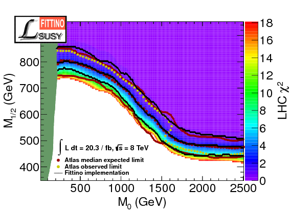
Figure 1: Comparison of the emulation of the ATLAS 0-Lepton search with the published ATLAS result. In red dots we show the Atlas median expected limit; the red lines denote the corresponding 1$\sigma$ uncertainty. The central black line is the result of the Fittino implementation described in the text. The upper and lower black curves are the corresponding 1$\sigma$ uncertainty. The yellow dots are the observed Atlas limit.

We reweight the events depending on their production channel according to NLO cross sections obtained from Prospino Beenakker:1996ed ; Beenakker:1996ch ; Beenakker:1997ut . Renormalisation and factorisation scales have been chosen such that the NLO+NLL resummed cross section normalisations Kulesza:2008jb ; Beenakker:2009ha ; Beenakker:2010nq ; Beenakker:2011fu ; Kramer:2012bx are reproduced for squark and gluino production.

For all predictions we take theoretical uncertainties into account, most of which are parameter dependent and reevaluated at every point in the MCMC. For the precision observables, they are given in Tab. 6. For the dark matter relic density we assume a theoretical uncertainty of $10\%$, for the neutralino-nucleon cross section entering the direct detection limits we assign $50\%$ uncertainty (see Ref. Bechtle:2012zk for a discussion of this uncertainty arinsing from pion-nuclueon form factors), for the Higgs boson mass prediction $2.4\%$, and for Higgs rates we use the uncertainties given by the LHC Higgs Cross Section Working Group Heinemeyer:2013tqa .

Table 6: Theoretical uncertainties of the precision observables used in the fit.

$a_{\mu}-a_{\mu}^{\mathrm{\mathrm{SM}}}$	$7\%$
$\sin^{2}\theta_{\mathrm{eff}}$	$0.05\%$
$m_{t}$	1 GeV
$m_{W}$	$0.01\%$
$\Delta m_{s}$	$24\%$
${\cal B}(B_{s}\to\mu\mu)$	$26\%$
${\cal B}(b\to s\gamma)$	$14\%$
${\cal B}(B\to\tau\nu)$	$20\%$

One common challenge for computing codes specifically developed for SUSY predictions is that they might not always exactly predict the most precise predictions of the SM value in the decoupling limit. The reason is that specific loop corrections or renormalisation conventions are not always numerically implemented in the same way, or that SM loop contributions might be missing from the SUSY calculation. In most cases these differences are within the theory uncertainty, or can be used to estimate those. One such case of interest for this fit occurs in the program FeynHiggs, which does not exactly reproduce the SM Higgs decoupling limit PrivateCommunicationSven as used by the LHC Higgs cross-section working group Heinemeyer:2013tqa . To compensate this, we rescale the Higgs production cross sections and partial widths of the SM-like Higgs boson. We determine the scaling factors by the following procedure PrivateCommunicationSven : We fix $\tan\beta=10$. We set all mass parameters of the MSSM (including the parameters $\mu$ and $m_{A}$ of the Higgs sector) to a common value $m_{\mathrm{SUSY}}$. We require all sfermion mixing parameters $A_{f}$ to be equal. We vary them by varying the ratio $X_{t}/m_{\mathrm{SUSY}}$, where $X_{t}=A_{t}-\mu/\tan\beta$. The mass of the Higgs boson becomes maximal for values of this ratio of about $\pm 2$. We scan the ratio between these values. In this way we find for each $m_{\mathrm{SUSY}}$ two parameter points which give a Higgs boson mass of about 125.5 GeV. One of these has negative $X_{t}$, the other positive $X_{t}$. We then determine the scaling factor by requiring that for $m_{\mathrm{SUSY}}=4$ TeV and negative $X_{t}$ the production cross sections and partial widths of the SM-like Higgs boson are the same as for a SM Higgs boson with the same mass of 125.5 GeV. We then determine the uncertainty on this scale factor by comparing the result with scale factors which we would have gotten by choosing $m_{\mathrm{SUSY}}=3$ TeV, $m_{\mathrm{SUSY}}=5$ TeV or a positive sign of $X_{t}$. This additional uncertainty is taking into account in the $\chi^{2}$ computation. By this procedure we derive scale factors between $0.95$ and $1.23$ with uncertainties of less than $0.6\%$.

4 Results

In Section 4.1, we show results based on the simplistic and common profile likelihood technique, which all frequentist fits, including us, have hitherto been employing. In Section 4.2 a full scan of the allowed parameter space for a stable vacuum is shown, before moving on to novel results from toy fits in Section 4.3.

4.1 Profile likelihood based results

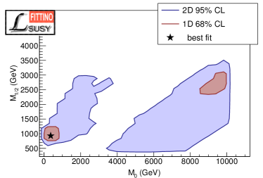
(a) 1$\,\sigma$ and 2$\,\sigma$ contour plot in in the ($M_{0}$,$\,M_{1/2}$)–plane for the Small Observable Set.

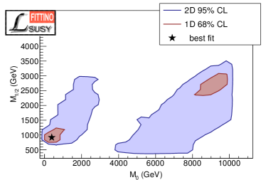
(b) 1$\,\sigma$ and 2$\,\sigma$ contour plot in in the ($M_{0}$,$\,M_{1/2}$)–plane for the Medium Observable Set.

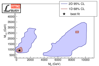
(c) 1$\,\sigma$ and 2$\,\sigma$ contour plot in the ($M_{0}$,$\,M_{1/2}$)–plane for the Large Observable Set.

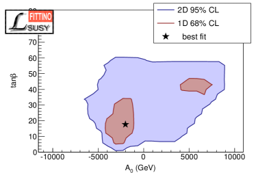
(d) 1$\,\sigma$ and 2$\,\sigma$ contour plot in the ($A_{0},\,\tan\beta$)–plane for the Medium Observable Set.

Figure 2: 1$\,\sigma$ and 2$\,\sigma$ contour plots for different projections and different observable sets. It can be seen that the preferred parameter region does not depend on the specific observable set.

In this section we describe the preferred parameter space region of the cMSSM and its physical properties. Since a truly complete frequentist determination of a confidence region would require not only to perform toy fits around the best fit point (as described in Section 2.2 and 4.3) but around every cMSSM parameter point in the scan, we rely here on the profile likelihood technique. This means, we show various projections of the 1D-$1\sigma$/1D-$2\sigma$/2D-$2\sigma$ regions defined as regions which satisfy $\Delta\chi^{2}<1/4/5.99$ respectively. In this context, profile likelihood means that out of the 5 physical parameters in the scan, the parameters not shown in a plot are profiled, i.e. a scan over the hidden dimensions is performed and for each selected visible parameter point the lowest $\chi^{2}$ value in the hidden dimensions is chosen. Obviously, no systematics nuisance parameters are involved, since all systematic uncertainties are given by relative or absolute Gaussian uncertainties, as discussed in Section 2. One should keep in mind that this correspondence is actually only exact when the observed distribution of $\chi^{2}$ values in a set of toy fits is truly $\chi^{2}$-distributed, which – as discussed in Section 4.3 – is not the case. Nevertheless, since the exact method is not computationally feasible, this standard method, as used in the literature in all previous frequentist results, gives a reasonable estimation of the allowed parameter space. In Section 4.3 more comparisons between the sets of toy fit results and the profile likelihood result will be discussed.

Note that for the discussion in this and the next section, we treat the region around the best fit point as “allowed”, even though, depending on the observable set, an exclusion of the complete model will be discussed in Section 4.3.

All five Higgs input parameterisations introduced in Section 3 lead to very similar results when interpreted with the profile likelihood technique. As an example, Figures 2(a) - 2(c) show the ($M_{0},\,M_{1/2}$)–projection of the best fit point, 1D-$1\sigma$ and 2D-$2\sigma$ regions for the Small, the Large and the Medium Observable Set. Thus, in the remainder of this section, we concentrate on results from the Medium Observable Set.

The ($M_{0},\,M_{1/2}$)–projection in Fig. 2(b) shows two disjoint regions. While in the region of the global $\chi^{2}$ minimum, values of less than 900 GeV for $M_{0}$ and less than 1300 GeV for $M_{1/2}$ are preferred at $1\sigma$, in the region of the secondary minimum values of more than 7900 GeV for $M_{0}$ and more than 2100 GeV for $M_{1/2}$ are favored (see also Tab. 7).

Table 7: Central values and $1\sigma$ uncertainties of the free model parameters at the global and secondary minimum when using the Medium Observable Set

Parameter	global minimum	secondary minimum
$M_{0}$ (GeV)	$387.4^{+481.7}_{-151.2}$	$8983.4^{+990.6}_{-1039.6}$
$M_{1/2}$ (GeV)	$918.2^{+297.7}_{-59.3}$	$2701.1^{+582.6}_{-560.5}$
$A_{0}$ (GeV)	$-2002.8^{+541.5}_{-1992.9}$	$5319.0^{+2339.8}_{-1357.9}$
$\tan\beta$	$17.7^{+16.8}_{-10.8}$	$43.2^{+5.5}_{-6.6}$
$m_{t}$ (GeV)	$174.3^{+1.1}_{-1.1}$	$172.1^{+0.6}_{-0.6}$

The different regions are characterised by different dominant dark matter annihilation mechanisms as shown in Fig. 3. Here we define the different regions similarly to Ref. Buchmueller:2014yva by the following kinematical conditions, which we have adapted such that each point of the 2D-$2\sigma$ region belongs to at least one region:

-	$\tilde{\tau}_{1}$ coannihilation:	${m_{\tilde{\tau}_{1}}}/{m_{\tilde{\chi}_{1}^{0}}}-1<0.15$
-	$\tilde{t}_{1}$ coannihilation:	${m_{\tilde{t}_{1}}}/{m_{\tilde{\chi}_{1}^{0}}}-1<0.2$
-	$\tilde{\chi}_{1}^{\pm}$ coannihilation:	${m_{\tilde{\chi}_{1}^{\pm}}}/{m_{\tilde{\chi}_{1}^{0}}}-1<0.1$
-	$A/H$ funnel:	$|{m_{A}}/{2m_{\tilde{\chi}_{1}^{0}}}-1|<0.2$
-	focus point region:	$|{\mu}/{m_{\tilde{\chi}_{1}^{0}}}-1|<0.4$

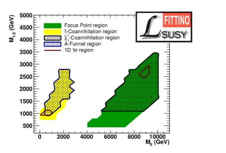
Figure 3: 2$\,\sigma$ region in the ($M_{0},\,M_{1/2}$)–plane for the Medium Observable Set. Regions with different dark matter annihilation mechanisms are indicated. The enclosed red areas denote the best fit regions shown in Fig. 2(b).

With these definitions each parameter point of the preferred 2D-$2\sigma$ region belongs either to the $\tilde{\tau}_{1}$ coannihilation or the focus point region. Additionally a subset of the points in the $\tilde{\tau}_{1}$ coannihilation region fulfills the criterion for the $A/H$-funnel, while some points of the focus point region fulfill the criterion for $\chi_{1}^{\pm}$ coannihilation. No point in the preferred 2D-$2\sigma$ region fulfills the criterion for $\tilde{t}_{1}$ coannihilation, due to relatively large stop masses.

At large $M_{0}$ and low $M_{1/2}$ a thin strip of our preferred 2D-$2\sigma$ region is excluded at 95% confidence level by ATLAS jets plus missing transverse momentum searches requiring exactly one lepton Aad:2015mia or at most one lepton and b-jets Aad:2014lra in the final state. Therefore an inclusion of these results in the fit is expected to remove this small part of the focus point region without changing any conclusion.

Also note that the parameter space for values of $M_{0}$ larger than $10$ TeV was not scanned such that the preferred 2D-$2\sigma$ focus point region is cut off at this value. Because the decoupling limit has already been reached at these large mass scales we do not expect significant changes in the predicted observable values when going to larger values of $M_{0}$. Hence we also expect the 1D-$1\sigma$ region to extend to larger values of $M_{0}$ than visible in Fig. 2(b) due to a low sampling density directly at the $10$ TeV boundary. For the same reason this cut is not expected to influence the result of the $p$-value calculation. If it does it would only lead to an overestimation of the $p$-value.

In the $\tilde{\tau}_{1}$ coannihilation region negative values of $A_{0}$ between $-4000$ GeV and $-1400$ GeV and moderate values of $\tan\beta$ between $6$ and $35$ are preferred, while in the focus point region large positive values of $A_{0}$ above 3400 GeV and large values of $\tan\beta$ above 36 are favored. This can be seen in the ($A_{0},\,\tan\beta$)–projection shown in Fig. 2(d) and in Tab. 7.

While the $\tilde{\tau}_{1}$ coannihilation region predicts a spin independent dark matter–nucleon scattering cross section which is well below the limit set by the LUX experiment, this measurement has a significant impact on parts of the focus point region for lightest supersymmetric particle (LSP) masses between 200 GeV and 1 TeV, as shown in Fig. 4. The plot also shows how the additional uncertainty of 50% on $\sigma_{\textrm{SI}}$ shifts the implemented limit compared to the original limit set by LUX. It can be seen that future improvements by about 2 orders of magnitude in the sensitivity of direct detection experiments, as envisaged e.g. for the future of the XENON 1T experiment 2012arXiv1206.6288A , could at least significantly reduce the remaining allowed parameter space even taking the systematic uncertainty into account, or finally discover SUSY dark matter.

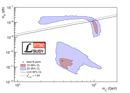
Figure 4: 1D$1\sigma$ and 2D$2\sigma$ regions in $m_{\tilde{\chi}_{1}^{0}}$-$\sigma_{SI}$ for the Medium Observable Set. The LUX exclusion is shown in addition. The dashed line indicates a $\chi^{2}$ contribution of 1.64 which corresponds to a $90\%$ CL upper limit. This line does not match the LUX exclusion line because we use a theory uncertainty of $50\%$ on $\sigma_{SI}$.

The predicted mass spectrum of the Higgs bosons and supersymmetric particles at the best fit point and in the one-dimensional 1$\sigma$ and 2$\sigma$ regions is shown in Fig. 5. Due to the relatively shallow minima of the fit a wide ranges of masses is allowed at $2\sigma$ for most of the particles. The masses of the coloured superpartners are predicted to lie above 1.5 TeV, but due to the focus point region also masses above 10 TeV are allowed at $1\sigma$. Similarly the heavy Higgs bosons have masses of about 1.5 TeV at the best fit point, but masses of about 6 TeV are preferred in the focus point region. The sleptons, neutralinos and charginos on the other hand can still have masses of a few hundred GeV.

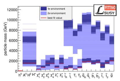
Figure 5: The Higgs and supersymmetric particle mass spectrum as predicted by our fit using the Medium set of Higgs observables.

A lightest Higgs boson with a mass as measured by the ATLAS and CMS collaborations can easily be accommodated, as shown in Fig. 6. As required by the signal strength measurements, it is predicted to be SM-like. Fig. 7 shows a comparison of the Higgs production cross sections for different production mechanisms in p-p collisions at a centre-of-mass energy of 14 TeV. These contain gluon-fusion (ggh), vector boson fusion (qqh), associated production (Wh, Zh), and production in assiciation with heavy quark flavours (bbh, tth). Compared to the SM prediction, the cMSSM predicts a slightly smaller cross section in all channels except the bbh channel. The predicted signal strengths $\mu$ in the different final states for p-p collisions at a centre-of-mass energy of 8 TeV is also slightly smaller than the SM prediction, as shown in Fig. 8. The current precision of these measurements does, however, not allow for a discrimination between the SM and the cMSSM based solely on measurements of Higgs boson properties.

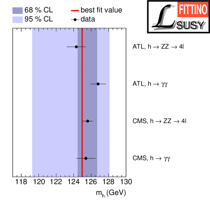
Figure 6: Our predicted mass of the light Higgs boson, together with the $1\,\sigma$ and $2\,\sigma$ ranges. The LHC measurements used in the fit are shown as well. Note that the correlated theory uncertainty of $\Delta m_{h_{theo}}=3$ GeV is not shown in the the plot. The relative smallness of the $68\%$ CL region of the fitted mass of $\Delta m_{h_{fit}}=1.1$ GeV is caused by constraints from other observables.

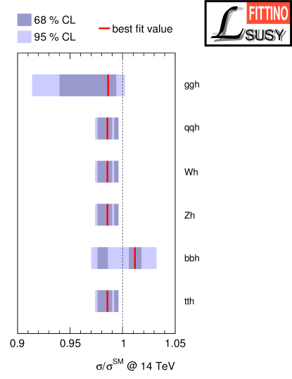
Figure 7: Predicted production cross sections at 14 TeV of the light Higgs boson relative to the SM value for a Higgs boson with the same mass

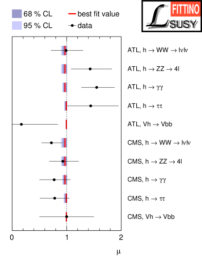
Figure 8: Our predicted $\mu$ values of the light Higgs boson relative to the SM value for a Higgs boson with the same mass. The measurements used in the fit are shown as well.

4.2 Vacuum stability

The scalar sector of the SM consists of just one complex Higgs doublet. In the cMSSM the scalar sector is dramatically expanded with an extra complex Higgs doublet, as well as the sfermions $\tilde{e}_{L,R},\,\tilde{\nu}_{L},\,\tilde{u}_{L,R},\,\tilde{d}_{L,R}$ of the first family, and correspondingly of the second and third families. Thus there are 25 complex scalar fields. The corresponding complete scalar potential $V_{cMSSM}$ is fixed by the five parameters: $(M_{0},\,M_{1/2},\,A,\,\tan\beta,\,\mathrm{sgn}(\mu))$. The minimal potential energy of the vacuum is obtained for constant scalar field values everywhere. Given a fixed set of these cMSSM parameters, it is a computational question to determine the minimum of $V_{cMSSM}$. Ideally this minimum should lead to a Higgs vacuum expectation such that SU(2)${}_{L}\times$U(1)${}_{Y}\to$U(1)_EM, as in the SM. However, it was observed early on in supersymmetric model building, that due to the extended scalar sector, some sfermions could obtain non-vanishing vacuum expectation values (vevs). There could be additional minima of the scalar potential which would break SU(3)_c and/or U(1)_EM and thus colour and/or charge Frere:1983ag ; Claudson:1983et ; Nilles:1982dy ; Derendinger:1983bz . If these minima are energetically higher than the conventional electroweak breaking minimum, then the latter is considered stable. If any of these minima are lower than the conventional minimum, our universe could tunnel into them. If the tunneling time is longer than the age of the Universe of 13.8 gigayears Ade:2013zuv , we denote our favored vacuum as metastable, otherwise it is unstable. However, this is only a rough categorisation. Since even if the tunneling time is shorter than the age of the universe, there is a finite probability, that it will have survived until today. When computing this probability, we set a limit of 10% survival probability. We wish to explore here the vacuum stability of the preferred parameter ranges of our fits.

The recent observation of the large Higgs boson mass requires within the cMSSM large stop masses and/or a large stop mass splitting. Together with the tuning of the lighter stau mass to favor the stau co-annihilation region (for the low $M_{0}$ fit region), this typically drives fits to favor a very large value of $|A_{0}|$ relative to $|M_{0}|$, cf. Tab. 7. (For alternative non-cMSSM models with a modified stop sector, see for example Auzzi:2012dv ; Evans:2012bf ; Chamoun:2014eda ; Staub:2015aea .) This is exactly the region, which typically suffers from the SM-like vacuum being only metastable, decaying to a charge- and/or colour-breaking (CCB) minimum of the potential Camargo-Molina:2013sta ; Blinov:2013fta .

For the purpose of a fit, in principle a likelihood value for the compatibility of the lifetime of the SM-like vacuum of a particular parameter point with the observation of the age of the Universe should be calculated and should be implemented as a one-sided limit. Unfortunately, the effort required to compute all the minima of the full scalar potential and to compute the decay rates for every point in the MCMC and to implement this in the likelihood function is beyond present capabilities Camargo-Molina:2013sta .

Effectively, whether or not a parameter point has an unacceptably short lifetime has a binary yes/no answer. Therefore, as a first step, and in the light of the results of the possible exclusion of the cMSSM in Section 4.3, we overlay our fit result from Section 4.1 over a scan of the lifetime of the cMSSM vacuum over the complete parameter space.

The systematic analysis of whether a potential has minima which are deeper than the desired vacuum configuration has been automated in the program Vevacious Camargo-Molina:2013qva . When restricting the analysis to only a most likely relevant subset of the scalar fields of the potential, i.e. not the full 25 complex scalar fields, and ignoring the calculation of lifetimes, this code runs sufficiently fast that we are able to present an overlay of which parameter points have CCB minima deeper than the SM-like minimum in Figures 9 and 10. However, only the stop and stau fields were allowed to have non-zero values in determining the overlays, in addition to the neutral components of the two complex scalar Higgs doublets. The $\tilde{\tau}_{L,R},\,\tilde{t}_{L,R}$ are suspected to have the largest effect Camargo-Molina:2013sta . The computation time when including more scalar fields which are allowed to vary increases exponentially. Thus the more detailed investigations below are restricted to a set of benchmark points. Note that the overlays in Figures 9 and 10 only show whether metastable vacua might occur at a given point, or whether the vacuum is instable at all. The actual lifetime is not yet considered in this step. See the further considerations below.

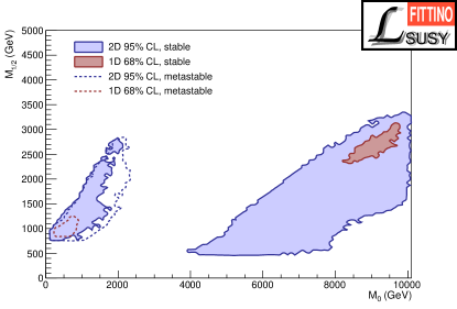
Figure 9: Preferred 1D-1$\sigma$ and 2D-2$\sigma$ regions in $M_{0}$-$M_{1/2}$ for the Medium Observable Set. The filled areas contain stable points, while the doted lines enclose points which are metastable but still might be very long-lived. The whole preferred 2D-2$\sigma$ focus point region leads to a stable vacuum, while the coannihilation region contains both stable and metastable points. There are no stable points in the preferred 1D-1$\sigma$ coannihilation region.

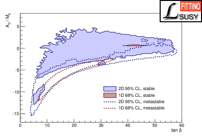
Figure 10: Preferred 1D-1$\sigma$ and 2D-2$\sigma$ regions in $\tan\beta$-$A_{0}/M_{0}$ for the Medium Observable Set. The filled areas contain stable points, while the doted lines enclose points which are metastable but still might be very long-lived. Points leading to a metastable vacuum have usually larger negative values of $A_{0}$ relative to $M_{0}$ when compared to points with a stable vacuum at the same $\tan\beta$. The part of the 1D-$1\sigma$ region which belongs to the focus point region fulfills $A_{0}/M_{0}\sim 0$ and is stable, while the part which belongs to the coannihilation region consists of points with relatively large negative values of $A_{0}/M_{0}$ and is metastable.

There are analytical conditions in the literature for whether MSSM parameter points could have dangerously deep CCB minima, see for example Nilles:1982dy ; Ibanez:1982qk ; AlvarezGaume:1983gj ; Claudson:1983et ; Derendinger:1983bz ; Kounnas:1983td ; Ibanez:1984vq ; Casas:1995pd . These can be checked numerically in a negligible amount of CPU time, while performing a fit. However, these conditions have been explicitly shown to be neither necessary nor sufficient Gunion:1987qv . In particular they have also been shown numerically to be neither necessary nor sufficient for the relevant regions of the cMSSM parameter space which we consider here Camargo-Molina:2013sta .

Since the exact calculation of the lifetime of a metastable SM-like vacuum is so computationally intensive, we unfortunately must restrict this to just the best-fit points of the stau co-annihilation and focus point regions of our the fit, as determined in Section 4.1. As an indicator, though, the extended $\tilde{\tau}_{1}$ co-annihilation region of the cMSSM investigated in Camargo-Molina:2013sta had SM-like vacuum lifetimes, which were all acceptably long compared to the observed age of the Universe.

The 1D1$\sigma$ best-fit points in Section 4.1 where checked for undesired minima, allowing, but not requiring, simultaneously for all the following scalar fields to have non-zero, real VEVs: $H_{d}^{0},H_{u}^{0},{\tilde{\tau}}_{L},{\tilde{\tau}}_{R},{\tilde{\nu}}_{{\mu}L},{\tilde{b}}_{L},{\tilde{b}}_{R},{\tilde{t}}_{L},{\tilde{t}}_{R}$. The focus point region best-fit point was found to have an absolutely stable SM-like minimum against tunneling to other minima, as no deeper minimum of $V_{cMSSM}$ was found at the 1-loop level. The SM-like vacuum of the best-fit $\tilde{\tau}_{1}$ co-annihilation point was found to be metastable, with a deep CCB minimum with non-zero stau and stop VEVs. Furthermore there were unbounded-from-below directions with non-zero values for the $\mu$-sneutrino scalar field in combination with nonzero values for both staus, or both sbottoms, or both chiralities of both staus and sbottoms. This does not bode very well for the absolute best-fit point of our cMSSM fit. However, further effects must be considered.

The parameter space of the MSSM which has directions in field space, where the tree-level potential is unbounded from below was systematically investigated in Ref. Casas:1995pd . We confirmed the persistence of the runaway directions at one loop with Vevacious out to field values of the order of twenty times the renormalisation scale. This is about the limit of trustworthiness of a fixed-order, fixed-renormalisation-scale calculation Camargo-Molina:2013qva . However, this is not quite as alarming as it may seem. The appropriate renormalisation scale for very large field values should be of the order of the field values themselves, and for field values of the order of the GUT scale, the cMSSM soft SUSY-breaking mass-squared parameters by definition are positive. Thus the potential at the GUT scale is bounded from below, as none of the conditions for unbounded-from-below directions given in Casas:1995pd can be satisfied without at least one negative mass-squared parameter. Note, even the Standard Model suffers from a potential which is unbounded from below at a fixed renormalisation scale. Though in the case of the SM it only appears at the one-loop level. Nevertheless, RGEs show that the SM is bounded from below at high energies Isidori:2001bm .

Furthermore, the calculation of a tunneling time out of a false minimum does not technically require that the Universe tunnels into a deeper minimum. In fact, the state which dominates tunneling is always a vacuum bubble, with a field configuration inside, which classically evolves to the true vacuum after quantum tunneling Coleman:1977py ; Callan:1977pt . Hence the lifetime of the SM-like vacuum of the stau co-annihilation best-fit point could be calculated at one loop even though the potential is unbounded from below at this level. The minimal energy barrier through which the SM-like vacuum of this point can tunnel is associated with a final state with non-zero values for the scalar fields $H_{d}^{0},\,H_{u}^{0},\,{\tilde{\tau}}_{L},\,{\tilde{\tau}}_{R}$, and ${\tilde{\nu}}_{{\mu}L}$. The lifetime was calculated by using the program Vevacious through the program CosmoTransitions Wainwright:2011kj to be roughly $e^{4000}\sim 10^{1700}$ times the age of the Universe. Therefore, we consider the $\tilde{\tau}_{1}$ coannihilation region best-fit point as effectively stable.

As well as asking whether a metastable vacuum has a lifetime at least as long as the age of the Universe at zero temperature, one can also ask whether the false vacuum would survive a high-temperature period in the early Universe. Such a calculation has been incorporated into Vevacious Camargo-Molina:2014pwa . In addition to the fact that the running of the Lagrangian parameters ensures that the potential is bounded from below at the GUT scale, the effects of non-zero temperature serve to bound the potential from below, as well. In fact the CCB minima of $V_{cMSSM}$ evaluated at the parameters of the stau co-annihilation best-fit point are no longer deeper than the configuration with all zero VEVs, which is assumed to evolve into the SM-like minimum as the Universe cools, for temperatures over about 2300 GeV. The probability of tunneling into the CCB state integrated over temperatures from 2300 GeV down to 0 GeV was calculated to be roughly $\exp(e^{-2000})$. So while having a non-zero-temperature decay width about $e^{-2000}/e^{-4000}=e^{+2000}$ times larger than the zero-temperature decay width, the SM-like vacuum, or its high-temperature precursor, of the stau co-annihilation best-fit point has a decay probability which is still utterly insignificant.

4.3 Toy based results

Pseudo datasets have been generated for a total of 7 different minima based on 6 different observable sets. For the Medium, Small and Combined Observable Sets, roughly 1000 sets of pseudo measurements have been taken into account, as well as for the observable set without the Higgs rates. For the Medium Observable Set, in addition to the best fit point, we also study the $p$-value of the local minimum in the focus point region. Due to relaxed requirements on the statistical uncertainty of a $p$-value in the range of ${\cal O}(0.5)$, as compared to ${\cal O}(0.05)$, we use only 125 pseudo datasets for the Large Observable Set. Finally, to study the importance of (g-2)_μ, a total of 500 pseudo datasets have been generated based on the best fit point for the Medium Observable Set without (g-2)_μ. A summary of all $p$-values with their statistical uncertainties and a comparison to the naive $p$-value according to the $\chi^{2}$-distribution for Gaussian distributed variables is shown in Tab. 8.

Table 8: Summary of $p$-values

Observable Set	$\chi^{2}$/ndf	naive $p$-value (%)	toy $p$-value (%)
Small	27.1/16	4.0	$1.9\pm 0.4$
Medium	30.4/22	10.8	$4.9\pm 0.7$
Combined	17.5/13	17.7	$8.3\pm 0.8$
Medium (Focus Point)	30.8/22	10.0	$7.8\pm 0.8$
Medium without (g-2)	18.1/21	64.1	$51\pm 3$
Observable Set without Higgs rates	15.5/9	7.8	$1.3\pm 0.4$

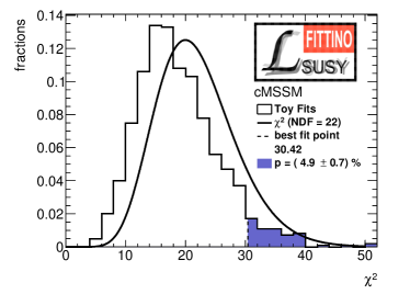
(a) Minimal $\chi^{2}$ values from toy fits using the Medium Observable Set.

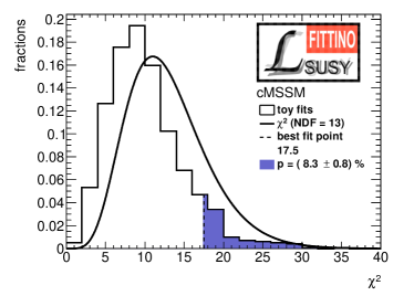
(b) Minimal $\chi^{2}$ values from toy fits using the Combined Observable Set.

Figure 11: Distribution of minimal $\chi^{2}$ values from toy fits using two different sets of Higgs observables. A $\chi^{2}$ distribution for Gaussian distributed variables is shown for comparison.

Figure 11(a) shows the $\chi^{2}$-distribution for the best fit point of the Medium Observable Set, from which we derive a $p$-value of ($4.9\pm 0.7$)%. As a comparison we also show the $\chi^{2}$-distribution for the pseudo fits using the Combined Observable Set in figure 11(b). Both distributions are significantly shifted towards smaller $\chi^{2}$-values compared to the corresponding $\chi^{2}$-distributions for Gaussian distributed variables. Several observables are responsible for the large deviation between the two distributions, as shown in Fig. 12(a), where the individual contributions of all observables to the minimum $\chi^{2}$ of all pseudo best fit points are plotted.

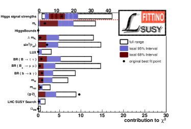
(a) Toy fits smeared around the global minimum in the $\tilde{\tau}$-coannihilation region.

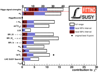
(b) Toy fits smeared around the local minimum in the focus point region.

Figure 12: Individual $\chi^{2}$ contributions of all observables/observable sets at the best fit points of the toy fits using the Medium Set of Higgs observables with observables smeared around the global and the local minimum of the observed $\chi^{2}$ contour. The predicted measurements at the best fit points of the individual pseudo data fits are used to derive the local CL intervals shown in the plots. These are compared with the individual $\chi^{2}$ contribution of each observable at the global or local minimum. Note the different scale shown on the top which is used for HiggsSignals, which contains 14 observables. Also note that $m_{h}$ contains contributions from $4$ measurements for this observable set.

First, HiggsBounds does not contribute significantly to the $\chi^{2}$ at any of the pseudo best-fit points, which is also the case for the original fit. The reason for this is, that for the majority of tested points, the $\chi^{2}$ contribution from HiggsBounds reflects the amount of violation of the LEP limit on the lightest Higgs boson mass by the model. Since the measurements of the Higgs mass by ATLAS and CMS lie significantly above this limit, it is extremely unlikely that in one of the pseudo datasets the Higgs mass is rolled such that the best fit point would receive a $\chi^{2}$ penalty due to the LEP limit. This effectively eliminates one degree of freedom from the fit. In addition, the predicted masses of $A,H$ and $H^{\pm}$ lie in the decoupled regime of the allowed cMSSM parameter space. Thus there are no contributions from heavy Higgs or charged Higgs searches as implemented in HiggsBounds.

The same effect is observed slightly less pronounced for the LHC and LUX limits, where the best fit points are much closer to the respective limits than in the case of HiggsBounds. Finally we observe that for each pseudo dataset the cMSSM can very well describe the pseudo measurement of the dark matter relic density, which further reduced the effective number of degrees of freedom.

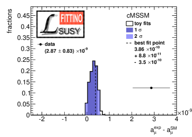
(a) Anomalous magnetic moment of the muon.

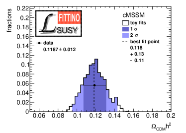
(b) Dark matter relic density.

Figure 13: Distribution of the predictions of the best fit points of the pseudo data fits for two different observables used in the fit, compared with the respective measurements.

Figure 12(a) also shows that the level of disagreement between measurement and prediction for $(g-2)_{\mu}$ is smaller in each single pseudo dataset than in the original fit with the real dataset. The 1-dimensional distribution of the pseudo best fit values of $(g-2)_{\mu}$ is shown in Fig. 13(a). The figure shows that under the assumption of our best fit point, not a single pseudo dataset would yield a prediction of $(g-2)_{\mu}$ that is consistent with the actual measurement. As a comparison, Fig. 13(b) shows the 1-dimensional distribution for the dark matter relic density, where the actual measurement can well be accommodated in any of the pseudo best fit scenarios. To further study the impact of $(g-2)_{\mu}$ on the $p$-value, we repeat the toy fits without this observable and get a $p$-value of $(51\pm 3)\%$. This shows that the relatively low $p$-value for our baseline fit is mainly due to the incompatibility of the $(g-2)_{\mu}$ measurement with large sparticle masses, which are however required by the LHC results.

Interestingly, under the assumption that the minimum in the focus point region is the true description of nature, we get a slightly better $p$-value (7.8%) than we get with the actual best fit point. Figure 12(b) shows the individual contributions to the pseudo best fit $\chi^{2}$ at the pseudo best fit points for the toy fits performed around the local minimum in the focus point region. There are two variables with higher average contributions compared to the global minimum: $m_{top}$ and the LHC SUSY search. In particular for the LHC SUSY search, the LHC contribution to the total $\chi^{2}$ is, on average, significantly higher than for the pseudo best fit points for the global minimum. The number of expected signal events for the minimum in the focus point region is 0, while it is $>0$ for the global minimum. Pseudo best fit points with smaller values of the mass parameters, in particular pseudo best fit points in the $\tilde{\tau}$-coannihilation region, tend to predict an expected number of signal events larger than zero. Since for the pseudo measurements based on the minimum in the focus point region an expectation of 0 is assumed, this naturally leads to a larger $\chi^{2}$ contribution from the ATLAS 0-$\ell$ analysis. The effect on the distribution of the total $\chi^{2}$ is shown in figure 14. Another reason might be that the focus point region is sampled more coarsely than the region around the global minimum. This increases the probability that the fit of the pseudo dataset misses the actual best fit point, due to our procedure of using only the points in the original MCMC. This effect should however only play a minor role, since the parameter space is still finely scanned and only a negligible fraction of scan points are chosen numerous times as best fit points in the pseudo data fits.

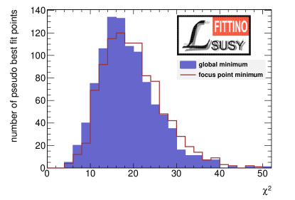
Figure 14: Comparison of the $\chi^{2}$ distributions obtained from toy fits using the global minimum and the local minimum in the focus point region of the Medium Observable Set.

To further verify that this effect is not only caused by the coarser sampling in the focus point region, we performed another set of 500 pseudo fits based on the global minimum, reducing the point density in the $\tilde{\tau}$-coannihilation region such that it corresponds to the point density around the local minimum in the focus point region. We find that the resulting $\chi^{2}$ distribution is slightly shifted with respect to the $\chi^{2}$ distribution we get from the full MCMC. The shift is, however, too small to explain the difference between $p$-values we find for the global minimum and the local minimum in the focus point region.

As an additional test, we investigate a simple toy model with only Gaussian observables and a single one-sided limit corresponding to the LHC SUSY search we use in our fit of the cMSSM. Also in this very simple model we find significantly different $\chi^{2}$ distributions for fits based on points in a region with/without a significant signal expectation for the counting experiment. We thus conclude that the true $p$-value for the local minimum in the focus point region is in fact higher than the true $p$-value for the global minimum of our fit.

In order to ensure that there are no more points with a higher $\chi^{2}$ and a higher $p$-value than the local minimum in the focus point region, we generate 200 pseudo datasets for two more points in the focus point region. The two points are the points with the highest/lowest $M_{0}$ in the local 1$\sigma$ region around the focus point minimum. We find that the $\chi^{2}$ distributions we get from these pseudo datasets are in good agreement with each other and also with the $\chi^{2}$ distribution derived from the pseudo experiments around the focus point minimum, and hence conclude that the local minimum in the focus point region is the point with the highest $p$-value in the cMSSM.

To study the impact of the Higgs rates on the $p$-value, and in order to compare to the observable sets used by other fit collaborations, which exclude the Higgs rate measurements from the fit on the basis that in the decoupling regime they do not play a vital role, we perform toy fits for the observable set without Higgs rates and derive a $p$-value of $(1.3\pm 0.4)\%$. In the decoupling limit, the cMSSM predictions for the Higgs rates are very close to the SM, so that the LHC is not able to distinguish between the two models based on Higgs rates measurements (see Fig. 8). Because of the overall good agreement between the Higgs rate measurements and the SM prediction, the inclusion of the Higgs rates in the fit improves the fit quality despite some tension between the ATLAS and CMS measurements.

As discussed in Section 2, it is important to understand the impact of the parametrisation of the measurements on the $p$-value. To do so, we compare our baseline fit with two more extreme choices. First, we use the Small Observable Set which combines $h\to\gamma\gamma$, $h\to ZZ$, and $h\to WW$ measurements but keeps ATLAS and CMS measurements separately. We use this choice because an official ATLAS combination is available. The equivalent corresponding CMS combination is produced independently by us. Using this observable set we get a $p$-value of $(1.9\pm 0.4)\%$. Here the cMSSM receives a $\chi^{2}$ penalty from the trend of the ATLAS signal strength measurements to values $\mu\geq 1$ and of the CMS measurements towards $\mu\leq 1$ in the three $h\to VV$ channels.

As a cross-check, we employ the Large Observable Set, which contains all available sub-channel measurements separately. Using this observable set, we get a $p$-value from the pseudo data fits of $(41.6\pm 4.4)\%$. As observed in Section 4.1, the Large Observable Set yields the same preferred parameter region as the Small, Medium and Combined Observable sets. Yet, its $p$-value from the pseudo data fits significantly differs.

To explain this interesting result we consider a simplified example: For $i=1,\dots,N$, let $x_{i}$ be Gaussian measurements with uncertainties $\sigma_{i}$ and corresponding model predictions $a_{i}(\mathbf{P})$ for a given parameter point $\mathbf{P}$. We assume that the measurements from $x_{n}$ to $x_{N}$ are uncombined measurements of the same observable; then $a_{i}=a_{n}$ for all $i\geq n$. There are now two obvious possibilities to compare measurements and predictions:

• We can compare each of the individual measurements with the corresponding model predictions by calculating

  $$\chi^{2}_{\mathrm{split}}=\sum_{i=1}^{N}\left(\frac{x_{i}-a_{i}}{\sigma_{i}}\right)^{2}.$$

  This would correspond to an approach where the model is confronted with all avaialable observables, irrespective of the question whether they measure independent quantities in the model or not. One example for such a situation would be the Large Observable Set of Higgs signal strength measurements, where several observables measure different detector effects, but the same physics.

• We can first combine the measurements $x_{i}$, $i\geq n$ to a measurement $\bar{x}$ which minimises the function

  $$f(x)=\sum_{i=n}^{N}\left(\frac{x_{i}-x}{\sigma_{i}}\right)^{2}$$ (9)

  and has an uncertainty of $\bar{\sigma}$ and then use this combination to calculate

  $$\chi^{2}_{\mathrm{combined}}=\sum_{i=1}^{n-1}\left(\frac{x_{i}-a_{i}}{\sigma_{i}}\right)^{2}+\left(\frac{\bar{x}-a_{n}}{\bar{\sigma}}\right)^{2}.$$ (10)

  This situation now corresponds to first calculating one physically meaningful quantity (e.g. a common signal strength for $h\to\gamma\gamma$ in all VBF categories, and all $gg\to h$ categories) and only then to confront the model to the combined measurement.

Plugging in the explicit expressions for ($\bar{x},\bar{\sigma}$), using $1/\bar{\sigma}^{2}=\sum_{i=n}^{N}(1/\sigma_{i}^{2})$ and defining $\chi^{2}_{\mathrm{data}}=f(\bar{x})$ one finds

$$\chi^{2}_{\mathrm{combined}}=\chi^{2}_{\mathrm{split}}-\chi^{2}_{\mathrm{data}}.$$ (11)

Hence doing the combination of the measurements before the fit is equivalent to using a $\chi^{2}$-difference which in turn is equivalent to the usage of a log-likelihood ratio. The numerator of this ratio is given by the likelihood $\mathcal{L}_{\mathrm{model}}$ of the model under study, e.g. the cMSSM. The denominator is given by the maximum of a phenomenological likelihood $\mathcal{L}_{\mathrm{pheno}}$ which depends directly on the model predictions $a_{i}$. These possess an expression as functions $a_{i}(\mathbf{P})$ of the model parameters $\mathbf{P}$ of $\mathcal{L}_{\mathrm{model}}$. Note that in $\mathcal{L}_{\mathrm{pheno}}$ however, the $a_{i}$ are treated as $n$ independent parameters. We now identify $\chi^{2}_{\mathrm{split}}\equiv-2\ln\mathcal{L}_{\mathrm{model}}$ and $\chi^{2}_{\mathrm{data}}\equiv-2\ln\mathcal{L}_{\mathrm{pheno}}$. When inserting $a_{i}(\mathbf{P})$, one is guaranteed to find

$$\mathcal{L}_{\mathrm{pheno}}(a_{1}(\mathbf{P}),\dots,a_{n}(\mathbf{P}))=\mathcal{L}_{\mathrm{model}}(\mathbf{P}).$$ (12)

Using these symbols, $\chi^{2}_{\mathrm{combined}}$ can be written as

$$\chi^{2}_{\mathrm{combined}}=-2\ln\frac{\mathcal{L_{\mathrm{model}}(\mathbf{P})}}{\mathcal{L}_{\mathrm{pheno}}(\hat{a}_{1},\dots,\hat{a}_{n})}\,,$$ (13)

where $\hat{a}_{1},\dots,\hat{a}_{n}$ maximise $\mathcal{L}_{\mathrm{pheno}}$. Note that in this formulation the model predictions $a_{i}$ do not necessarily need to correspond directly to measurements used in the fit, as it is the case for our example. For instance the model predictions $a_{i}$ might contain cross sections and branching ratios which are constrained by rate measurements.

Using $\mathrm{ndf}_{\mathrm{split}}=N$, $\mathrm{ndf}_{\mathrm{combined}}=n$ and $\mathrm{ndf}_{\mathrm{data}}=N-n$ Eq. (11) implies

$$\frac{\chi^{2}_{\mathrm{split}}}{\mathrm{ndf_{split}}}=\frac{\chi^{2}_{\mathrm{combined}}}{\mathrm{ndf_{combined}}+N-n}+\frac{\chi^{2}_{\mathrm{data}}}{\mathrm{ndf_{data}}+n}.$$ (14)

The more uncombined measurements are used, the larger $N-n$ gets and the less the $p$-value depends on the first term on the right hand side, which measures the agreement between data and model. At the same time, the $p$-value depends more on the second term on the right hand which measures the agreement within the data. Especially, for $n$ fixed and $N\to\infty$:

$$\frac{\chi^{2}_{\mathrm{split}}}{\mathrm{ndf_{split}}}=\frac{\chi^{2}_{\mathrm{data}}}{\mathrm{ndf_{data}}}\,.$$ (15)

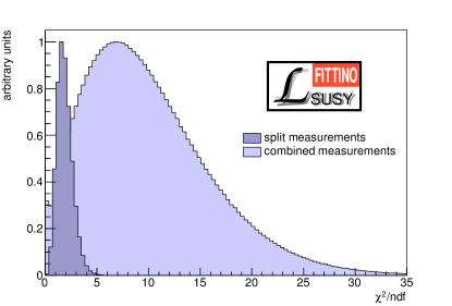
Figure 15: Numerical example showing the distribution of $\chi^{2}/\mathrm{ndf}$ using combined and split measurements. Using split measurements smaller values of $\chi^{2}/\mathrm{ndf}$ are obtained. Because in this example all measurements are Gaussian, this is equivalent to larger $p$-values. We call the effect of obtaining larger $p$-values when using split measurements the dilution of the $p$-value.

Since in the case of purely statistical fluctuations of the split measurements around the combined value the agreement within the data is unlikely to be poor, the expectation is

$$\frac{\chi^{2}_{\mathrm{data}}}{\mathrm{ndf_{data}}}\approx 1$$ (16)

even if there was a deviation between the model predictions and the physical combined observables. So most of the time the $p$-value will get larger when uncombined measurements are used, hiding deviations between model and data. As a numerical example Fig. 15 shows toy distributions of $\frac{\chi^{2}_{\mathrm{combined}}}{\mathrm{ndf_{combined}}}$ and $\frac{\chi^{2}_{\mathrm{split}}}{\mathrm{ndf_{split}}}$ for one observable (n=1), ten measurements (N=10) and a $3\sigma$ deviation between the true value and the model prediction. We call this effect dilution of the $p$-value. It explains the large $p$-value for the Large Observable Set by the overall good agreement between the uncombined measurements.

On the other hand if there is some tension within the data, which might in this hypothetical example be caused purely by statistical or experimental effects, the “innocent” model is punished for these internal inconsistencies of the data. This is observed here for the Medium Observable Set and Small Observable Set. Hence, and in order to incorporate our assumption that ATLAS and CMS measured the same Higgs boson, we produce our own combination of corresponding ATLAS and CMS Higgs mass and rate measurements. We also assume that custodial symmetry is preserved but do not assume that $h\to\gamma\gamma$ is connected to $h\to WW$ and $h\to ZZ$ as in the official ATLAS combination used in Small Observable Set. We call the resulting observable set Combined Observable Set. Note that for simplicity we also combine channels for which the cMSSM model predictions might differ due to different efficiencies for the different Higgs production channels. This could be improved in a more rigorous treatment. For instance the $\chi^{2}$ could be defined by Eq. (13) using a likelihood $\mathcal{L}_{\mathrm{pheno}}$ which contains both the different Higgs production cross sections and the different Higgs branching ratios as free parameters $a_{i}$.

Using the Combined Observable Set we get a $p$-value of $(8.3\pm 0.8)\%$, which is significantly smaller than the diluted $p$-value of $(41.6\pm 4.4)\%$ for the Large Observable Set. The good agreement within the data now shows up in a small $\chi^{2}/\mathrm{ndf}$ of $68.1/65$ for the combination but no longer affects the $p$-value of the model fit. On the other hand the $p$-value for the Combined Observable Set is larger than the one for the Medium Observable Set, because the tension between the ATLAS and CMS measurements is not included. This tension can be quantified by producing an equivalent ATLAS and CMS combination not from the Large Observable Set but from the Medium Observable Set giving a relatively bad $\chi^{2}/\mathrm{ndf}$ of $10.9/6$.

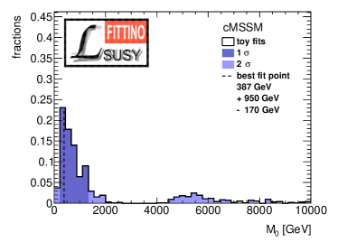
(a)

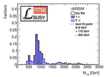
(b)

Figure 16: Distribution of the pseudo best fit values for 16(a) $M_{0}$ and 16(b) $M_{1/2}$.

Finally, as discussed briefly in Section 2, we employ the Medium Observable Set again to compare the preferred parts of the parameter space according to the profile likelihood technique (Fig. 2(b)) with the parameter ranges that are preferred according to our pseudo fits. In Fig. 16(a) and 16(b) we show the 1-dimensional distributions of the pseudo best fit values for $M_{0}$ and $M_{1/2}$. The $68\%$ and $95\%$ CL regions according to the total pseudo best fit $\chi^{2}$ are shown. As expected by the non-Gaussian behaviour of our fit, some differences between the results obtained by the profile likelihood technique and the pseudo fit results can be observed. For the pseudo fits, in both parameters $M_{0}$ and $M_{1/2}$, the $95\%$ CL range is slightly smaller compared to the allowed range according to the profile likelihood. Considering the fits of the pseudo datasets, $M_{0}$ is limited to values $<8.5$ TeV and $M_{1/2}$ is limited to values $<2.7$ TeV, while the profile likelihood technique yields upper limits of $10$ TeV and $3.5$ TeV, roughly. The differences are relatively small compared to the size of the preferred parameter space, and may well be an effect of the limited number of pseudo datasets that have been considered; the use of the profile likelihood technique for the derivation of the preferred parameter space can therefore be considered to give reliable results. However, as discussed above, in order to get an accurate estimate for the $95\%$-CL regions, the $p$-value would have to be evaluated at every single point in the parameter space.

5 Conclusions

In this paper we present what we consider the final analysis of the cMSSM in light of the LHC Run 1 with the program Fittino.

In previous iterations of such a global analysis of the cMSSM, or any other more general SUSY model, the focus was set on finding regions in parameter space that globally agree with a certain set of measurements, either using frequentist or bayesian statistics. However, these analyses show that a constrained model such as the cMSSM has become rather trivial: because of the decoupling behaviour at sufficiently high SUSY mass scales the phenomenology resembles that of the SM with dark matter. This does however not disqualify the cMSSM as a valid model of Nature. In addition, there are undeniable fine-tuning challenges, but also these do not statistically disqualify the model. Therefore, before abandoning the cMSSM, we apply one crucial test, which it has not been performed before: we calculate the $p$-value of the cMSSM through toy tests.

A likelihood ratio test of the cMSSM against the SM would be meaningless, since the SM cannot acommodate dark matter. Thus we apply a goodness-of-fit test of the cMSSM. As in every likelihood test (also in likelihood ratio tests), the sensitivity of the test towards the validity of the model depends on the number of degrees of freedom in the observable set, while the sensitivity towards the preferred parameter range does not. Thus, when calculating the $p$-value of the cMSSM, it is important that the observable set is chosen carefully. First, only such observables should be considered for which the cMSSM predictions are, in principle, sensitive to the choice of the model parameters, independent of the actually measured values of the observables. This excludes e.g. many LEP/SLD precision observables, for which the cMSSM by construction always predicts the SM value for any parameter value. Second, it is important that observables are combined whenever the corresponding cMSSM predictions are not independent. Otherwise the resulting $p$-value would be too large by construction. It should be noted that the allowed parameter space for all observable sets studied here is virtually identical. It is only the impact on the $p$-value which varies.

In order to study this dependence, several observable sets are studied. The main challenge arises from the Higgs rate measurements. Since the cMSSM Higgs rate predictions are, in principle, very sensitive to the choice of model parameters, the corresponding measurements have to be included in a global fit. Using the preferred observable sets “combined” and “medium” (as described in Section 4.3 and Tab. 8), we calculate a $p$-value of the cMSSM of 4.9% and 8.4%, respectively. In addition, the cMSSM is excluded at the 98.7% CL if Higgs rate measurements are omitted. The main reason for these low $p$-values is the tension between the direct sparticle search limits from the LHC and the measured value of the muon anomalous magnetic moment $(g-2)_{\mu}$. If e.g. $(g-2)_{\mu}$ is removed from the fit, the $p$-value of the cMSSM increases to about 50%. However, there is no justification for arbitrarily removing one variable a posteriori. On the other hand, the observable sets could be artificially chosen to be too detailed, such that there are many measurements for which the model predictions cannot be varied individually. This is the case for the Large Observable Set of Higgs rate observables in Tab. 8, the inclusion of which does thus not represent a methodologically stringent test of the $p$-value of the cMSSM.

Thus, the main result of this analysis is that the cMSSM is excluded at least at the 90% CL for reasonable choices of the observable set.

The best-fit point is in the $\tilde{\tau}$-coannihilation region at $M_{0}\approx 500$ GeV, with a secondary minimum in the focus-point region at $M_{1/2},M_{0}\gg 2$ TeV. A comparison of the $p$-values of coannihilation and focus-point regions can serve as an estimate of a likelihood-ratio test between a cMSSM at $M_{0}\approx 500$ GeV which can be tested at the LHC, and a “SM with dark matter” with squark and gluino masses beyond about 5 TeV. Since the focus point manifests a more linear relation between observables and input parameters in the toy fits, and thus a more $\chi^{2}$-distribution like behaviour, it reaches a slightly higher $p$-value than the $\tilde{\tau}$-coannihilation region. This shows that even the best-fit region offers no statistically relevant advantage over the “SM with dark matter”. Thus, we can conclude that the cMSSM is not only excluded at the 90% to 95% CL, but that it is also statistically mostly indistinguishable from a hypothetical SM with dark matter.

In addition to this main result, we apply the first complete scan of the possibility of the existence of charge or colour-breaking minima within a global fit of the cMSSM. In addition, we calculate the lifetime of the best fit points. We find that the focus-point best-fit-region is stable, while the $\tilde{\tau}$-coannihilation best-fit region is either stable or metastable, with a lifetime significantly longer than the age of the Universe.

It is important to note that the exclusion of the cMSSM at the 90% CL or more does in general not apply to less restricted SUSY models. The combination of measurements requiring low slepton and gaugino mass scales, such as $(g-2)_{\mu}$, and the high mass scales preferred by the SM-like Higgs and the non-observation of coloured sparticles at the LHC puts the cMSSM under extreme tension. In the cMSSM these mass scales are connected. A more general SUSY model where these scales are decoupled, and preferably also with a complete decoupling of the third generation sleptons and squarks from the first and second generation, would easily circumvent this tension.

Therefore, the future of SUSY searches at the LHC should emphasize the coverage of any phenomenological scenario which allows sleptons, and preferably also third generation squarks, to remain light, while the other sparticles can become heavy. Many loopholes with light SUSY states still exist, as analyses as in CMS-PAS-SUS-13-020 show, and there exist potentially promising experimental anomalies which could be explained by more general SUSY models Khachatryan:2015lwa ; Aad:2015wqa ; ATLAS-CONF-2014-033 .

On the other hand, the analysis presented here shows that SUSY does not directly point towards a non-SM-like light Higgs boson. The uncertainty on the predictions of ratios of partial decay widths and other observables at the LHC are significantly smaller than the direct uncertainty of the LHC Higgs rate measurements. This is because of the high SUSY mass scale, also for third generation squarks, imposed by the combination of the cMSSM and the direct SUSY particle search limits. These do not allow the model to vary the light Higgs boson properties sufficiently to make use of the experimental uncertainty in the Higgs rate measurements. This might change for a more general SUSY model, but there is no direct hint in this direction. The predicted level of deviation of the light Higgs boson properties from the SM prediction at the ${\cal O}(1\%)$ level is not accessible even at a high-luminosity LHC and requires an $e^{+}e^{-}$ collider.

In summary, we find that the undeniable freedom in choosing the observable set – before looking at the experimental values of the results – introduces a remaining softness into the exclusion of the cMSSM. Therefore, while we might have preferred to find SUSY experimentally, we find that at least we can almost complete the second most revered task of a physics measurement: with the combination of astrophysical, precision collider and energy frontier measurements in a global frequentist analysis we (softly) kill the cMSSM.

- (1) J. Wess, B. Zumino, Nucl.Phys. B70, 39 (1974)
- (2) Y. Golfand, E. Likhtman, JETP Lett. 13, 323 (1971)
- (3) R. Haag, J.T. Lopuszanski, M. Sohnius, Nucl. Phys. B88, 257 (1975)
- (4) P. Langacker, M.x. Luo, Phys.Rev. D44, 817 (1991)
- (5) U. Amaldi, W. de Boer, H. Furstenau, Phys.Lett. B260, 447 (1991)
- (6) J.R. Ellis, S. Kelley, D.V. Nanopoulos, Phys.Lett. B260, 131 (1991)
- (7) H.P. Nilles, M. Srednicki, D. Wyler, Phys. Lett. B120, 346 (1983)
- (8) L.E. Ibanez, G.G. Ross, Phys. Lett. B110, 215 (1982)
- (9) E. Gildener, Phys.Rev. D14, 1667 (1976)
- (10) M. Veltman, Acta Phys.Polon. B12, 437 (1981)
- (11) R. Barbieri, G. Giudice, Nucl.Phys. B306, 63 (1988)
- (12) P. Fayet, Phys.Lett. B69, 489 (1977)
- (13) G.R. Farrar, P. Fayet, Phys.Lett. B76, 575 (1978)
- (14) H. Goldberg, Phys.Rev.Lett. 50, 1419 (1983)
- (15) J.R. Ellis, J. Hagelin, D.V. Nanopoulos, K.A. Olive, M. Srednicki, Nucl.Phys. B238, 453 (1984)
- (16) H.P. Nilles, Phys.Rept. 110, 1 (1984)
- (17) S.P. Martin, A Supersymmetry primer. [Adv. Ser. Direct. High Energy Phys.18,1(1998)]
- (18) P. Fayet, Nucl.Phys. B90, 104 (1975)
- (19) P. Fayet, J. Iliopoulos, Phys.Lett. B51, 461 (1974)
- (20) P. Fayet, Phys.Lett. B64, 159 (1976)
- (21) S. Ferrara, L. Girardello, F. Palumbo, Phys.Rev. D20, 403 (1979)
- (22) D.Z. Freedman, P. van Nieuwenhuizen, S. Ferrara, Phys. Rev. D13, 3214 (1976)
- (23) E. Cremmer, B. Julia, J. Scherk, S. Ferrara, L. Girardello, P. van Nieuwenhuizen, Nucl. Phys. B147, 105 (1979)
- (24) E. Cremmer, S. Ferrara, L. Girardello, A. Van Proeyen, Nucl. Phys. B212, 413 (1983)
- (25) G.L. Kane, C.F. Kolda, L. Roszkowski, J.D. Wells, Phys. Rev. D49, 6173 (1994)
- (26) L. Girardello, M.T. Grisaru, Nucl.Phys. B194, 65 (1982)
- (27) S. Dimopoulos, H. Georgi, Nucl.Phys. B193, 150 (1981)
- (28) H.P. Nilles, Phys.Lett. B115, 193 (1982)
- (29) R. Barbieri, S. Ferrara, C.A. Savoy, Phys. Lett. B119, 343 (1982)
- (30) A.H. Chamseddine, R.L. Arnowitt, P. Nath, Phys.Rev.Lett. 49, 970 (1982)
- (31) S.K. Soni, H.A. Weldon, Phys. Lett. B126, 215 (1983)
- (32) L.J. Hall, J.D. Lykken, S. Weinberg, Phys. Rev. D27, 2359 (1983)
- (33) S.S. AbdusSalam, et al., Eur. Phys. J. C71, 1835 (2011)
- (34) P. Bechtle, K. Desch, M. Uhlenbrock, P. Wienemann, Eur.Phys.J. C66, 215 (2010)
- (35) P. Bechtle, B. Sarrazin, K. Desch, H.K. Dreiner, P. Wienemann, et al., Phys.Rev. D84, 011701 (2011)
- (36) P. Bechtle, T. Bringmann, K. Desch, H. Dreiner, M. Hamer, et al., JHEP 1206, 098 (2012)
- (37) P. Bechtle, K. Desch, H.K. Dreiner, M. Hamer, M. Krämer, et al., PoS EPS-HEP2013, 313 (2013)
- (38) O. Buchmueller, R. Cavanaugh, D. Colling, A. De Roeck, M. Dolan, et al., Eur.Phys.J. C71, 1583 (2011)
- (39) O. Buchmueller, R. Cavanaugh, D. Colling, A. de Roeck, M. Dolan, et al., Eur.Phys.J. C71, 1634 (2011)
- (40) O. Buchmueller, R. Cavanaugh, D. Colling, A. De Roeck, M. Dolan, et al., Eur.Phys.J. C71, 1722 (2011)
- (41) O. Buchmueller, R. Cavanaugh, A. De Roeck, M. Dolan, J. Ellis, et al., Eur.Phys.J. C72, 1878 (2012)
- (42) O. Buchmueller, R. Cavanaugh, A. De Roeck, M. Dolan, J. Ellis, et al., Eur.Phys.J. C72, 2020 (2012)
- (43) O. Buchmueller, R. Cavanaugh, M. Citron, A. De Roeck, M. Dolan, et al., Eur.Phys.J. C72, 2243 (2012)
- (44) O. Buchmueller, M. Dolan, J. Ellis, T. Hahn, S. Heinemeyer, et al., Eur.Phys.J. C74, 2809 (2014)
- (45) O. Buchmueller, R. Cavanaugh, A. De Roeck, M. Dolan, J. Ellis, et al., Eur.Phys.J. C74, 2922 (2014)
- (46) O. Buchmueller, R. Cavanaugh, M. Citron, A. De Roeck, M. Dolan, et al., The NUHM2 after LHC Run 1. (2014). arXiv:1408.4060 [hep-ph]
- (47) K.J. de Vries, et al., (2015)
- (48) E.A. Bagnaschi, et al., (2015)
- (49) J. Ellis, Eur.Phys.J. C74, 2732 (2014)
- (50) G. Bertone, D.G. Cerdeno, M. Fornasa, R. Ruiz de Austri, C. Strege, et al., JCAP 1201, 015 (2012)
- (51) C. Strege, G. Bertone, D. Cerdeno, M. Fornasa, R. Ruiz de Austri, et al., JCAP 1203, 030 (2012)
- (52) C. Strege, G. Bertone, F. Feroz, M. Fornasa, R. Ruiz de Austri, et al., JCAP 1304, 013 (2013)
- (53) C. Balazs, A. Buckley, D. Carter, B. Farmer, M. White, Eur.Phys.J. C73, 2563 (2013)
- (54) C. Beskidt, W. de Boer, D. Kazakov, F. Ratnikov, JHEP 1205, 094 (2012)
- (55) C. Beskidt, W. de Boer, D.I. Kazakov, Phys. Lett. B738, 505 (2014)
- (56) R. Lafaye, T. Plehn, M. Rauch, D. Zerwas, Eur.Phys.J. C54, 617 (2008)
- (57) C. Adam, J.L. Kneur, R. Lafaye, T. Plehn, M. Rauch, et al., Eur.Phys.J. C71, 1520 (2011)
- (58) S. Henrot-Versillé, R. Lafaye, T. Plehn, M. Rauch, D. Zerwas, et al., Phys.Rev. D89, 055017 (2014)
- (59) B.C. Allanach, K. Cranmer, C.G. Lester, A.M. Weber, JHEP 0708, 023 (2007)
- (60) B. Allanach, Phys.Rev. D83, 095019 (2011)
- (61) B. Allanach, T. Khoo, C. Lester, S. Williams, JHEP 1106, 035 (2011)
- (62) R.R. de Austri, R. Trotta, L. Roszkowski, JHEP 0605, 002 (2006)
- (63) A. Fowlie, A. Kalinowski, M. Kazana, L. Roszkowski, Y.S. Tsai, Phys.Rev. D85, 075012 (2012)
- (64) L. Roszkowski, E.M. Sessolo, Y.L.S. Tsai, Phys.Rev. D86, 095005 (2012)
- (65) A. Fowlie, M. Kazana, K. Kowalska, S. Munir, L. Roszkowski, et al., Phys.Rev. D86, 075010 (2012)
- (66) K. Kowalska, et al., Phys.Rev. D87(11), 115010 (2013)
- (67) K. Kowalska, L. Roszkowski, E.M. Sessolo, JHEP 1306, 078 (2013)
- (68) K. Kowalska, L. Roszkowski, E.M. Sessolo, S. Trojanowski, JHEP 1404, 166 (2014)
- (69) L. Roszkowski, E.M. Sessolo, A.J. Williams, JHEP 1408, 067 (2014)
- (70) K. Kowalska, L. Roszkowski, E.M. Sessolo, S. Trojanowski, A.J. Williams, Looking for supersymmetry: 1 Tev WIMP and the power of complementarity in LHC and dark matter searches. (2015), URL http://inspirehep.net/record/1385134/files/arXiv:1507.07446.pdf
- (71) S. Cassel, D.M. Ghilencea, S. Kraml, A. Lessa, G.G. Ross, JHEP 05, 120 (2011)
- (72) U. Ellwanger, G. Espitalier-Noel, C. Hugonie, JHEP 09, 105 (2011)
- (73) A. Kaminska, G.G. Ross, K. Schmidt-Hoberg, JHEP 11, 209 (2013)
- (74) D.M. Ghilencea, Phys. Rev. D89(9), 095007 (2014)
- (75) H. Baer, V. Barger, D. Mickelson, M. Padeffke-Kirkland, Phys. Rev. D89(11), 115019 (2014)
- (76) P. Bechtle, et al., How alive is constrained SUSY really? (2014), URL http://inspirehep.net/record/1323294/files/arXiv:1410.6035.pdf
- (77) A. Fowlie, Bayesian approach to investigating supersymmetric models. (2013), URL http://etheses.whiterose.ac.uk/id/eprint/4742
- (78) A.A. Markov, Science in Context 19, 591 (2006), URL http://journals.cambridge.org/article_S0269889706001074
- (79) N. Metropolis, A.W. Rosenbluth, M.N. Rosenbluth, A.H. Teller, E. Teller, J. Chem. Phys. 21, 1087 (1953)
- (80) W.K. Hastings, Biometrika 57, 97 (1970)
- (81) G. Aad, et al., JHEP 1409, 176 (2014)
- (82) G. Bennett, et al., Phys.Rev. D73, 072003 (2006)
- (83) M. Davier, A. Hoecker, B. Malaescu, Z. Zhang, Eur.Phys.J. C71, 1515 (2011)
- (84) S. Schael, et al., Phys.Rept. 427, 257 (2006)
- (85) ATLAS Collaboration, CDF Collaboration, CMS Collaboration, D0 Collaboration, First combination of Tevatron and LHC measurements of the top-quark mass. (2014). arXiv:1403.4427 [hep-ex]
- (86) Tevatron Electroweak Working Group, 2012 Update of the Combination of CDF and D0 Results for the Mass of the W Boson. (2012). arXiv:1204.0042 [hep-ex]
- (87) J. Beringer, et al., Phys.Rev. D86, 010001 (2012)
- (88) CMS and LHCb Collaborations, Combination of results on the rare decays from the CMS and LHCb experiments. (2013). CMS-PAS-BPH-13-007, LHCb-CONF-2013-012, CERN-LHCb-CONF-2013-012
- (89) Y. Amhis, et al., Averages of B-Hadron, C-Hadron, and tau-lepton properties as of early 2012 . (2012). arXiv:1207.1158 [hep-ex]
- (90) P.A.R. Ade, et al., Astron. Astrophys. 571, A16 (2014)
- (91) D. Akerib, et al., Phys.Rev.Lett. 112, 091303 (2014)
- (92) ALEPH, DELPHI, L3 and OPAL collaborations, (2001), URL http://lepsusy.web.cern.ch/lepsusy/www/inos_moriond01/charginos_pub.html
- (93) P. Bechtle, O. Brein, S. Heinemeyer, G. Weiglein, K.E. Williams, Comput. Phys. Commun. 181, 138 (2010)
- (94) P. Bechtle, O. Brein, S. Heinemeyer, G. Weiglein, K.E. Williams, Comput. Phys. Commun. 182, 2605 (2011)
- (95) P. Bechtle, O. Brein, S. Heinemeyer, O. Stål, T. Stefaniak, et al., PoS CHARGED2012, 024 (2012)
- (96) P. Bechtle, O. Brein, S. Heinemeyer, O. Stål, T. Stefaniak, et al., Eur.Phys.J. C74(3), 2693 (2014)
- (97) P. Bechtle, S. Heinemeyer, O. Stål, T. Stefaniak, G. Weiglein, Eur.Phys.J. C74(2), 2711 (2014)
- (98) P. Bechtle, S. Heinemeyer, O. Stål, T. Stefaniak, G. Weiglein, JHEP 1411, 039 (2014)
- (99) G. Aad, et al., Phys. Rev. Lett. 114, 191803 (2015)
- (100) G. Aad, et al., Phys.Lett. B726, 88 (2013)
- (101) S. Chatrchyan, et al., Phys.Rev. D89, 092007 (2014)
- (102) CMS Collaboration, Combination of standard model Higgs boson searches and measurements of the properties of the new boson with a mass near 125 GeV. CMS-PAS-HIG-13-005 (2013)
- (103) ATLAS Collaboration, Search for the Standard Model Higgs boson in H->tau tau decays in proton-proton collisions with the ATLAS detector. ATLAS-CONF-2012-160, ATLAS-COM-CONF-2012-196 (2012)
- (104) ATLAS collaboration, Search for the bb decay of the Standard Model Higgs boson in associated W/ZH production with the ATLAS detector. ATLAS-CONF-2013-079, ATLAS-COM-CONF-2013-080 (2013)
- (105) S. Chatrchyan, et al., JHEP 1401, 096 (2014)
- (106) S. Chatrchyan, et al., Nature Phys. 10, 557 (2014)
- (107) CMS Collaboration, Updated measurements of the Higgs boson at 125 GeV in the two photon decay channel. CMS-PAS-HIG-13-001 (2013)
- (108) W. Porod, Comput.Phys.Commun. 153, 275 (2003)
- (109) W. Porod, F. Staub, Comput.Phys.Commun. 183, 2458 (2012)
- (110) S.P. Martin, M.T. Vaughn, Phys.Rev. D50, 2282 (1994)
- (111) D.M. Pierce, J.A. Bagger, K.T. Matchev, R.j. Zhang, Nucl.Phys. B491, 3 (1997)
- (112) S. Heinemeyer, W. Hollik, G. Weiglein, Comput.Phys.Commun. 124, 76 (2000)
- (113) T. Hahn, S. Heinemeyer, W. Hollik, H. Rzehak, G. Weiglein, Phys.Rev.Lett. 112(14), 141801 (2014)
- (114) G. Degrassi, S. Heinemeyer, W. Hollik, P. Slavich, G. Weiglein, Eur.Phys.J. C28, 133 (2003)
- (115) B. Allanach, A. Djouadi, J. Kneur, W. Porod, P. Slavich, JHEP 0409, 044 (2004)
- (116) S. Heinemeyer, W. Hollik, H. Rzehak, G. Weiglein, Eur.Phys.J. C39, 465 (2005)
- (117) F. Mahmoudi, Comput.Phys.Commun. 180, 1579 (2009)
- (118) W. Porod, F. Staub, A. Vicente, Eur.Phys.J. C74(8), 2992 (2014)
- (119) G. Belanger, F. Boudjema, A. Pukhov, A. Semenov, Comput.Phys.Commun. 149, 103 (2002)
- (120) G. Belanger, F. Boudjema, A. Pukhov, A. Semenov, Comput.Phys.Commun. 174, 577 (2006)
- (121) P. Gondolo, J. Edsjo, P. Ullio, L. Bergstrom, M. Schelke, et al., JCAP 0407, 008 (2004)
- (122) N. Nguyen, D. Horns, T. Bringmann, AstroFit: An Interface Program for Exploring Complementarity in Dark Matter Research. (2012). arXiv:1202.1385 [astro-ph]
- (123) M. Bahr, S. Gieseke, M. Gigg, D. Grellscheid, K. Hamilton, et al., Eur.Phys.J. C58, 639 (2008)
- (124) S. Ovyn, X. Rouby, V. Lemaitre, DELPHES, a framework for fast simulation of a generic collider experiment. (2009). arXiv:0903.2225 [hep-ph]
- (125) W. Beenakker, R. Hopker, M. Spira, PROSPINO: A Program for the production of supersymmetric particles in next-to-leading order QCD. (1996). arXiv:hep-ph/9611232
- (126) W. Beenakker, R. Hopker, M. Spira, P.M. Zerwas, Nucl. Phys. B492, 51 (1997)
- (127) W. Beenakker, M. Krämer, T. Plehn, M. Spira, P.M. Zerwas, Nucl. Phys. B515, 3 (1998)
- (128) A. Kulesza, L. Motyka, Phys. Rev. Lett. 102, 111802 (2009)
- (129) W. Beenakker, S. Brensing, M. Krämer, A. Kulesza, E. Laenen, I. Niessen, JHEP 12, 041 (2009)
- (130) W. Beenakker, S. Brensing, M. Krämer, A. Kulesza, E. Laenen, I. Niessen, JHEP 08, 098 (2010)
- (131) W. Beenakker, S. Brensing, M. Krämer, A. Kulesza, E. Laenen, L. Motyka, I. Niessen, Int. J. Mod. Phys. A26, 2637 (2011)
- (132) M. Krämer, A. Kulesza, R. van der Leeuw, M. Mangano, S. Padhi, T. Plehn, X. Portell, (2012)
- (133) S. Heinemeyer, et al., Handbook of LHC Higgs Cross Sections: 3. Higgs Properties. (2013). arXiv:1307.1347 [hep-ph]
- (134) T. Hahn, S. Heinemeyer. private communication
- (135) G. Aad, et al., JHEP 04, 116 (2015)
- (136) G. Aad, et al., JHEP 10, 24 (2014)
- (137) E. Aprile, XENON1T collaboration, The XENON1T Dark Matter Search Experiment. (2012). arXiv:1206.6288 [astro-ph]
- (138) J.M. Frere, D.R.T. Jones, S. Raby, Nucl. Phys. B222, 11 (1983)
- (139) M. Claudson, L.J. Hall, I. Hinchliffe, Nucl. Phys. B228, 501 (1983)
- (140) J.P. Derendinger, C.A. Savoy, Nucl. Phys. B237, 307 (1984)
- (141) R. Auzzi, A. Giveon, S.B. Gudnason, T. Shacham, JHEP 01, 169 (2013)
- (142) J.A. Evans, Y. Kats, JHEP 04, 028 (2013)
- (143) N. Chamoun, H.K. Dreiner, F. Staub, T. Stefaniak, JHEP 08, 142 (2014)
- (144) F. Staub, P. Athron, U. Ellwanger, R. Grober, M. Muhlleitner, P. Slavich, A. Voigt, (2015)
- (145) J. Camargo-Molina, B. O’Leary, W. Porod, F. Staub, JHEP 1312, 103 (2013)
- (146) N. Blinov, D.E. Morrissey, JHEP 03, 106 (2014)
- (147) J. Camargo-Molina, B. O’Leary, W. Porod, F. Staub, Vevacious: A Tool For Finding The Global Minima Of One-Loop Effective Potentials With Many Scalars. (2013). arXiv:1307.1477 [hep-ph]
- (148) L.E. Ibanez, Nucl. Phys. B218, 514 (1983)
- (149) L. Alvarez-Gaume, J. Polchinski, M.B. Wise, Nucl. Phys. B221, 495 (1983)
- (150) C. Kounnas, A.B. Lahanas, D.V. Nanopoulos, M. Quiros, Nucl. Phys. B236, 438 (1984)
- (151) L.E. Ibanez, C. Lopez, C. Munoz, Nucl. Phys. B256, 218 (1985)
- (152) J. Casas, A. Lleyda, C. Muñoz, Nucl.Phys. B471, 3 (1996)
- (153) J. Gunion, H. Haber, M. Sher, Nucl.Phys. B306, 1 (1988)
- (154) G. Isidori, G. Ridolfi, A. Strumia, Nucl.Phys. B609, 387 (2001)
- (155) S.R. Coleman, Phys.Rev. D15, 2929 (1977)
- (156) J. Callan, Curtis G., S.R. Coleman, Phys.Rev. D16, 1762 (1977)
- (157) C.L. Wainwright, Comput.Phys.Commun. 183, 2006 (2012)
- (158) J. Camargo-Molina, B. Garbrecht, B. O’Leary, W. Porod, F. Staub, Phys.Lett. B737, 156 (2014)
- (159) CMS Collaboration, Phenomenological MSSM interpretation of the CMS 7 and 8 TeV results. CMS-PAS-SUS-13-020 (2014)
- (160) V. Khachatryan, et al., JHEP 04, 124 (2015)
- (161) G. Aad, et al., Eur. Phys. J. C75(7), 318 (2015)
- (162) ATLAS Collaboration, Measurement of the production cross section in proton-proton collisions at TeV with the ATLAS detector. ATLAS-CONF-2014-033 (2014)