A new discrete monotonicity formula with application to a two-phase free boundary problem in dimension two

Abstract.

We continue the analysis of the two-phase free boundary problems initiated in [14], where we studied the linear growth of minimizers in a Bernoulli type free boundary problem at the non-flat points and the related regularity of free boundary. There, we also defined the functional

$$\varphi_{p}(r,u,x_{0})=\frac{1}{r^{4}}\int_{B_{r}(x_{0})}\frac{|{\nabla}u^{+}(x)|^{p}}{|x-x_{0}|^{N-2}}dx\int_{B_{r}(x_{0})}\frac{|{\nabla}u^{-}(x)|^{p}}{|x-x_{0}|^{N-2}}dx$$

where $x_{0}$ is a free boundary point, i.e. $x_{0}\in\partial\{u>0\}$ and $u$ is a minimizer of the functional

$$J(u):=\int_{\Omega}|\nabla u|^{p}+\lambda_{+}^{p}\,\chi_{\{u>0\}}+\lambda_{-}^{p}\,\chi_{\{u\leq 0\}},$$

for some bounded smooth domain $\Omega\subset\mathbb{R}^{N}$ and positive constants $\lambda_{\pm}$ with $\Lambda:=\lambda_{+}^{p}-\lambda^{p}_{-}>0$.

Here we show the discrete monotonicity of $\varphi_{p}(r,u,x_{0})$ in two spatial dimensions at non-flat points, when $p$ is sufficiently close to 2, and then establish the linear growth. A new feature of our approach is the anisotropic scaling argument discussed in Section 4.

1. Introduction

Let $\Omega\subset\mathbb{R}^{2}$ be a bounded planar domain such that any function in the Sobolev space $W^{1,p}(\Omega)$ has well-defined trace and $p\in(2,2+\varepsilon)$, for a small, fixed $\varepsilon>0$. Assume that $u$ is a local minimizer of

(1.1) $$J(u):=\int_{\Omega}|\nabla u|^{p}+\lambda_{+}^{p}\,\chi_{\{u>0\}}+\lambda_{-}^{p}\,\chi_{\{u\leq 0\}},\quad u-g\in W_{0}^{1,p}(\Omega),$$

where $\lambda_{+}$ and $\lambda_{-}$ are positive constants such that $\lambda_{+}^{p}-\lambda_{-}^{p}>0$ and $g\in W^{1,p}(\Omega)$ is a prescribed boundary datum. In what follows $\chi_{U}$ denotes the characteristic function of the set $U\subset\mathbb{R}^{2}$.

The variational problem for (1.1) is called the Bernoulli-type free boundary problem and it models a number of interesting phenomena, notably planar cavitational flow of one or two perfect fluids (see [4] Chapter 9.11), the equilibrium configuration for heat or electrostatic energy optimization in higher dimensions, (e.g. heat flow with power Fourier law) and the dynamics of non-Newtonian fluids when the velocity obeys the power law ${\bf v}=\nabla\psi|\nabla\psi|^{\frac{1}{s}-1}$ where $\psi$ is a stream function. Notice that $s=1$ corresponds to Newtonian fluids and $s$ is a physical parameter, see [3].

For $p=2$ both the one phase and the two-phase problems have been extensively studied for variational [2] as well as viscosity solutions [10]. There is a significant difference between the one phase and two-phase problems stipulated by a sign change of $u$ across the free boundary. The main and only known method for proving the optimal regularity for the two-phase problem is based on the monotonicity formula of Alt, Caffarelli and Friedman [2] given by

(1.2) $$\varphi(r,x_{0})=\frac{1}{r^{4}}\int_{B_{r}(x_{0})}\frac{|{\nabla}u^{+}(x)|^{2}}{|x-x_{0}|^{N-2}}dx\int_{B_{r}(x_{0})}\frac{|{\nabla}u^{-}(x)|^{2}}{|x-x_{0}|^{N-2}}dx,$$

where $r>0$ and $x_{0}\in\partial\{u>0\}$. It is well-known that if $u$ is a minimizer of (1.1) and $u^{+}:=\max\{0,u\}$ and $u^{-}:=-\min\{0,u\}$, then $\varphi(r,x_{0})$ is a non-decreasing function of $r$. The monotonicity of $\varphi$, combined with the coherent growth of $\frac{1}{t}\fint_{B_{t}(x_{0})}u^{+}$ and $\frac{1}{t}\fint_{B_{t}(x_{0})}u^{-}$, for $x_{0}\in\partial\{{u>0}\}$, gives uniform local upper linear bound for $u$, see [2].

The key ingredient in the proof of the monotonicity formula in [2] is the following geometric property of the eigenvalues of the Laplace-Beltrami operator on the unit sphere $\partial B_{1}$: let $\gamma_{1},\gamma_{2}$ be the characteristic numbers corresponding to two complementary domains $\Gamma_{1},\Gamma_{2}$ on $\partial B_{1}$, that is

$$\gamma_{i}(\gamma_{i}+N-2):=\inf_{v\in W^{1,2}_{0}(\Gamma_{i})}\frac{\int_{\Gamma_{i}}|\nabla_{\theta}v|^{2}}{\int_{\Gamma_{i}}v^{2}},\quad i=1,2,$$

then

(1.3) $$\gamma_{1}+\gamma_{2}\geq 2$$

and the equality holds if and only if $\Gamma_{1},\Gamma_{2}$ are two complementary hemispheres, see [10], Chapter 12.

Note that in two spatial dimensions $\gamma_{i}$ is the square root of the eigenvalue corresponding to the portion $\Gamma_{i}$ of the unit circle.

In Section 7 we present some results related to the characteristc numbers and the eigenvalues of the $p$-Laplace-Beltrami operator for $p\neq 2$.

There are fewer results established for $p\neq 2$ for the two-phase problem. A partial result on the optimal regularity of $u$ is given in [19] under a smallness assumption on the Lebesgue density of the set $\{u\leq 0\}$, and recently has been extended to a more general class of functionals in [5].

Our paper contributes in the direction of optimal regularity and monotonicity formula techniques. More precisely, we show that in two spatial dimensions $N=2$ (and for $p$ sufficiently close to 2) the functional

(1.4) $$\varphi_{p}(r,u,x_{0}):=\frac{1}{r^{4}}\int_{B_{r}(x_{0})}|\nabla u^{+}|^{p}\,\int_{B_{r}(x_{0})}|\nabla u^{-}|^{p}$$

is discrete monotone (see Theorem 2.1 for the precise statement). Here $r>0$ is small and $x_{0}\in\Gamma:=\partial\{u>0\}$, being $\Gamma$ the free boundary. Consequently, we prove that $\varphi_{p}$ is bounded if the free boundary is not flat at $x_{0}$.

In fact, we establish a dichotomy for $\varphi_{p}$: either the free boundary is smooth at $x_{0}$ or $\varphi_{p}$ is discrete monotone.

For this, we introduce a suitable notion of flatness for the free boundary points characterizing the flat points. It follows from the results of [20, 21] that at such points the free boundary must be regular provided that $u$ is also a viscosity solution in the sense of Definition 6.1, see also the discussion in Section 6. The fact that minimizers of $J$ are viscosity solutions has been established in [14].

On the other hand, at non-flat points, we prove that $\varphi_{p}$ is discrete monotone and we deduce from this the linear growth of $u$ near these points.

In the subsequent section, we present our main results. A detailed plan about the organization of the paper will then be presented at the end of Section 2.

2. Main Results

In this section we formulate our main results. We will denote by $\Gamma:=\partial\{u>0\}$ the free boundary. Fix $x_{0}\in\Gamma$ and $h>0$, and consider the slab

(2.1) $$S(h;x_{0},\nu):=\{x\in\mathbb{R}^{n}:-h<(x-x_{0})\cdot\nu<h\}$$

where $\nu$ is a unit vector. Let $h_{\min}(x_{0},r,\nu)$ be the minimal height of the slab in the unit direction $\nu$ containing the free boundary in $B_{r}(x_{0})$, i.e.

(2.2) $$h_{\min}(x_{0},r,\nu):=\inf\{h:\partial\{u>0\}\cap B_{r}(x_{0})\subset S(h;x_{0},\nu)\cap B_{r}(x_{0})\}.$$

If we set

(2.3) $$h(x_{0},r):=\inf_{\nu\in\mathbb{S}^{n}}h_{\min}(x_{0},r,\nu)$$

then $h(x_{0},r)$ is non-decreasing in $r$.

Theorem to follow deals with the points where the free boundary is not sufficiently flat.

Theorem 2.1.

Let $u$ be a local minimizer of the functional $J$ defined in (1.1). Then, there exist tame constants $p_{0}>2$, $r_{0}>0$ and $h_{0}>0$ such that if

(2.4) $$2<p<p_{0}\quad and\quad r<r_{0}$$

(2.5) then the inequality $$h(x_{0},r)\geq h_{0}r,\quad{\mbox{ for }}x_{0}\in\Gamma\cap B_{3r},$$

implies that

(2.6) $$\varphi_{p}(r,u,x_{0})\leq\varphi_{p}(3r,u,x_{0}),$$

where $h(x,r)$ is defined by (2.3) and $\varphi_{p}$ by (1.4).

Theorem 2.1 says that if at the level $r$ the free boundary is not sufficiently flat then the $\varphi_{p}$ energy at the level $r$ is controlled by the same energy at the tripled level $3r$.

It is worthwhile to point out that in the proof of Theorem 2.1 we use a compactness argument based on an anisotropic scaling in order to assure the non-degeneracy of an appropriately scaled function, thus avoiding the use of the knowledge of the linear growth from [14].

As a consequence, we have the following:

Theorem 2.2.

Let $u$ be a local minimizer of the functional $J$ defined in (1.1), and let $x_{0}\in\Gamma$ be a non-flat point of the free boundary, i.e. for any $r<r_{0}$ we have $h(x_{0},r)\geq h_{0}r$, where $r_{0}$ is given by Theorem 2.1.

Then, $u$ has linear growth near $x_{0}$.

Observe that we always have that $u^{+}$ and $u^{-}$ have comparable rates of growth from the free boundary, thanks to Corollary 3.6, i.e.

$$\frac{1}{r}\fint_{B_{r}(x_{0})}u^{+}\sim\frac{1}{r}\fint_{B_{r}(x_{0})}u^{-}.$$

In order to conclude that each of these terms is bounded we apply Theorem 2.1 to infer that the product $\frac{1}{r^{2}}\fint_{B_{r}(x_{0})}u^{+}\fint_{B_{r}(x_{0})}u^{-}$ is also bounded. This is where $\varphi_{p}$ enters into the game and provides the necessary bound, see Section 5.

Outline

In Section 3 we collect some basic material that we will use throughout the paper. We also show a coherence result (see Proposition 3.1, P.4) by using a different strategy with respect to the case $p=2$ (see [2]), that we think has an independent interest.

Sections 4 and 5 are devoted to the proofs of Theorems 2.1 and 2.2.

In Section 6 we discuss the fact that any minimizer of the functional in (1.1) is also a viscosity solution, according to Definition 6.1. This, together with the notion of slab flatness, will allow us to apply the regularity theory developed in [20, 21] for viscosity solutions.

Finally, in Section 7 we recall some results concerning the relation between the characteristic numbers corresponding to two complementary cones for $p\neq 2$.

Notations

$C,C_{0},C_{N},\cdots$	generic constants,
$\overline{U}$	closure of a set $U$,
$\partial U$	boundary of a set $U$,
$B_{r}(x),B_{r}$	ball centered at $x$ with radius $r>0$, $B_{r}:=B_{r}(0)$,
$\Gamma$	the free boundary $\partial\{u>0\}$,
$\Gamma_{\pm}$	$B_{1}\cap\partial\{u^{\pm}>0\}$,
$\displaystyle\fint$	mean value integral,
$\omega_{N}$	volume of unit ball,
$\lambda(u)$	$\lambda_{+}^{p}\,\chi_{\{u>0\}}+\lambda_{-}^{p}\,\chi_{\{u\leq 0\}}$,
$\Lambda=\lambda_{+}^{p}-\lambda^{p}_{-}$	Bernoulli constant.

3. Technicalities

In this section we gather some basic facts that we shall use in the forthcoming sections. One of the important results to be proved is the coherence estimate (3.1). In the case $p=2$ this estimate was showed in [2] (see Theorem 4.1 there), and the proof uses the Poisson representation formula, that we do not have for $p\not=2$. However, a combination of the methods from [2], [13] and [18] will give the result.

3.1. Some basic properties of the local minimizers of $J$

In the proposition to follow all claims are valid in any dimension.

Proposition 3.1.

Let $u\in W^{1,p}(\Omega)$ be a local minimizer of $J$. Then

• $\Delta_{p}u^{\pm}\geq 0$ in the sense of distributions and $\Delta_{p}u=0$ in $\{u>0\}\cup\{u<0\}$,

• there is $c_{0}>0$ such that if

  $$\limsup_{r\to 0}\frac{|B_{r}(x_{0})\cap\{u<0\}|}{|B_{r}(x_{0})|}\leq c_{0},\quad x_{0}\in\Gamma,$$

  then $u$ has linear growth near $x_{0}$ depending only on $\frac{1}{c_{0}}$ times some tame constant,

• $\nabla u\in L^{q}$ locally, for any finite $q>1$, and $u$ is locally log-Lipschitz continuous,

• for any $D\Subset\Omega$ there exist $\bar{r}>0$ and $C>0$ depending on $p,\sup|u|,\operatorname{dist}(D,\partial\Omega)$ such that for any $x_{0}\in\Gamma\cap B_{1}$

  (3.1) $$\left|\fint_{\partial B_{r}(x_{0})}u\right|\leq Cr,\quad{\mbox{ for any }}r\leq\bar{r}.$$

Remark 3.2.

Note that P.4 in Proposition 3.1 says that either both  $\frac{1}{r}\fint_{\partial B_{r}(x_{0})}u^{+}$ and $\frac{1}{r}\fint_{\partial B_{r}(x_{0})}u^{-}$ go to $+\infty$ as $r\to 0$ or they both remain bounded.

Remark 3.3.

We stress on the fact that the results in Proposition 3.1 hold in any dimension

Proof.

P.1 follows from a standard comparison of $u$ and $u+\varepsilon\varphi$ for a suitable smooth compactly supported function $\varphi$, and the proof of P.2 can be found in [19].

Now we focus on the proofs of P.3 and P.4. For this, we observe that it is enough to show that

(3.2) $${\mbox{locally }}\,{\nabla}u\in BMO.$$

Indeed, if this is true then $\nabla u\in L^{q}$ locally, for any $1<q<+\infty$. Moreover, the log-Lipschitz estimate follows from [11], Theorem 3. This proves P.3.

Also, $u$ is continuous and

$$\lim_{r\to 0}\fint_{\partial B_{r}(x_{0})}u=0\quad\mbox{ for any}x_{0}\in\Gamma.$$

Now, we notice that, for $\varepsilon>0$,

$$\left|\frac{1}{\varepsilon^{N-1}}\int_{B_{\varepsilon}(x)}\nabla u(x)\cdot\frac{x-x_{0}}{|x-x_{0}|}\,dx\right| = \left|\frac{1}{\varepsilon^{N-1}}\int_{B_{\varepsilon}(x)}\left(\nabla u(x)-\fint_{B_{\varepsilon}(x)}\nabla u\right)\cdot\frac{x-x_{0}}{|x-x_{0}|}\,dx\right|$$

$$\leq \varepsilon\left(\frac{1}{\varepsilon^{N}}\int_{B_{\varepsilon}(x)}\left|\nabla u(x)-\fint_{B_{\varepsilon}(x)}\nabla u\right|\,dx\right)\longrightarrow 0,$$

as $\varepsilon\to 0$, thanks to the BMO estimate in (3.2). Thus

$$\frac{1}{r^{N-1}}\int_{\partial B_{r}(x)}u = \int_{0}^{r}\left(\frac{d}{dt}\int_{\partial B_{1}}u(x_{0}+t\omega)\,d\mathcal{H}^{1}\right)\,dt$$

$$= \int_{0}^{r}\frac{1}{t^{N-1}}\int_{\partial B_{t}}{\nabla}u(x_{0}+\nu)\cdot\nu\,d\mathcal{H}^{1}\,dt=$$

$$= \int_{0}^{r}\frac{1}{t^{N-1}}\frac{d}{dt}\left(\int_{B_{t}(x_{0})}{\nabla}u(x)\cdot\frac{x-x_{0}}{|x-x_{0}|}\,dx\right)\,dt=$$

$$= \frac{1}{r^{N-1}}\int_{B_{r}(x_{0})}{\nabla}u(x)\frac{x-x_{0}}{|x-x_{0}|}\,dx+(N-1)\int_{0}^{r}\frac{1}{t^{N}}\int_{B_{t}(x_{0})}{\nabla}u(x)\frac{x-x_{0}}{|x-x_{0}|}\,dx\,dt$$

$$= \frac{1}{r^{N-1}}\int_{B_{r}(x_{0})}\left[{\nabla}u(x)-\fint_{B_{r}(x_{0})}{\nabla}u\right]\frac{x-x_{0}}{|x-x_{0}|}\,dx$$

$$+(N-1)\int_{0}^{r}\frac{1}{t^{N}}\int_{B_{t}(x_{0})}\left[{\nabla}u(x)-\fint_{B_{t}(x_{0})}{\nabla}u\right]\frac{x-x_{0}}{|x-x_{0}|}\,dx\,dt.$$

Therefore, the BMO estimate in (3.2) yields

$$\left|\frac{1}{r^{N-1}}\int_{\partial B_{r}(x)}u\right|\leq 3r\|{\nabla}u\|_{BMO},$$

which gives the desired result in P.4.

Hence, it remains to show (3.2), that is that locally ${\nabla}u\in BMO$. In order to provce it, fix $R\geq r>0$ and let $v$ be the solution of $\Delta_{p}v=0$ in $B_{2R}(x_{0})$ and $v=u$ on $\partial B_{2R}(x_{0})$. If follows from [12] p. 100 that

$$\int_{B_{2R}(x_{0})}|{\nabla}(u-v)|^{p}\leq CR^{N},$$

for some tame constant $C>0$. Notice that, by Hölder inequality,

(3.3) $$\int_{B_{2R}(x_{0})}|{\nabla}(u-v)|^{2}\leq CR^{N},$$

up to renaming $C$.

Now, we denote by

$$({\nabla}u)_{x_{0},\rho}:=\fint_{B_{\rho}(x_{0})}\nabla u,$$

and we observe that, using Hölder inequality,

(3.4) $$\begin{split}\int_{B_{r}(x_{0})}|({\nabla}v)_{x_{0},r}-({\nabla}u)_{x_{0},r}|^{2}&\,=\int_{B_{r}(x_{0})}\left|\frac{1}{|B_{r}|}\left(\int_{B_{r}(x_{0})}{\nabla}v-{\nabla}u\right)\right|^{2}\\ &\,\leq\left(\int_{B_{r}(x_{0})}|\nabla v-\nabla u|\right)^{2}\\ &\,\leq\int_{B_{r}(x_{0})}|\nabla v-\nabla u|^{2}.\end{split}$$

Furthermore, we have the following Campanato growth type estimate (see [13] Theorem 5.1)

(3.5) $$\int_{B_{r}(x_{0})}|{\nabla}v-({\nabla}v)_{x_{0},R}|^{2}\lesssim\left(\frac{r}{R}\right)^{N+\alpha}\int_{B_{R}(x_{0})}|{\nabla}v-({\nabla}v)_{x_{0},R}|^{2},$$

where the symbol $\lesssim$ means that the inequality is true up to a positive constant.

Therefore, using (3.3), (3.4) and (3.5), we have

$$\int_{B_{r}(x_{0})}|{\nabla}u-({\nabla}u)_{x_{0},r}|^{2} \lesssim \int_{B_{r}(x_{0})}|{\nabla}u-{\nabla}v|^{2}+\int_{B_{r}(x_{0})}|{\nabla}v-({\nabla}v)_{x_{0},r}|^{2}$$

$$+\int_{B_{r}(x_{0})}|({\nabla}v)_{x_{0},r}-({\nabla}u)_{x_{0},r}|^{2}$$

$$\lesssim \int_{B_{r}(x_{0})}|{\nabla}u-{\nabla}v|^{2}+\int_{B_{r}(x_{0})}|{\nabla}v-({\nabla}v)_{x_{0},r}|^{2}$$

$$\lesssim \int_{B_{r}(x_{0})}|{\nabla}u-{\nabla}v|^{2}+\left(\frac{r}{R}\right)^{N+\alpha}\int_{B_{R}(x_{0})}|{\nabla}v-({\nabla}v)_{x_{0},R}|^{2}$$

$$\lesssim \int_{B_{r}(x_{0})}|{\nabla}u-{\nabla}v|^{2}$$

$$+\left(\frac{r}{R}\right)^{N+\alpha}\left[\int_{B_{R}(x_{0})}|{\nabla}v-{\nabla}u|^{2}+\int_{B_{R}(x_{0})}|{\nabla}u-({\nabla}u)_{x_{0},R}|^{2}\right]$$

$$+\left(\frac{r}{R}\right)^{N+\alpha}\int_{B_{R}(x_{0})}|({\nabla}u)_{x_{0},R}-({\nabla}v)_{x_{0},R}|^{2}$$

$$\lesssim \int_{B_{r}(x_{0})}|{\nabla}u-{\nabla}v|^{2}$$

$$+\left(\frac{r}{R}\right)^{N+\alpha}\left[\int_{B_{R}(x_{0})}|{\nabla}v-{\nabla}u|^{2}+\int_{B_{R}(x_{0})}|{\nabla}u-({\nabla}u)_{x_{0},R}|^{2}\right]$$

$$\lesssim \int_{B_{R}(x_{0})}|{\nabla}u-{\nabla}v|^{2}+\left(\frac{r}{R}\right)^{N+\alpha}\int_{B_{R}(x_{0})}|{\nabla}u-({\nabla}u)_{x_{0},R}|^{2}$$

$$\lesssim (R)^{N}+\left(\frac{r}{R}\right)^{N+\alpha}\int_{B_{R}(x_{0})}|{\nabla}u-({\nabla}u)_{x_{0},R}|^{2}.$$

Now, we define

$$\psi(r):=\sup\limits_{t\leq r}\int\limits_{B_{t}(x_{0})}|{\nabla}u-({\nabla}u)_{x_{0},t}|^{2}.$$

It follows from [13] that

$$\psi(r)\leq A\left(\frac{r}{R}\right)^{N+\alpha}\psi(R)+BR^{N}$$

for some positive constants $A$, $B$ and $\alpha$. Applying Lemma 2.1 from [18] Chapter 3 we conclude that there exist $c>0$ and $R_{0}>0$ such that

$$\psi(r)\leq cr^{N}\left(\frac{\psi(R)}{R^{N}}+B\right)$$

for all $r\leq R\leq R_{0}$, and hence

$$\int_{B_{r}(x_{0})}|{\nabla}u-({\nabla}u)_{x_{0},r}|^{2}\leq Cr^{N}$$

for some tame constant $C>0$. This shows that $\nabla u$ is locally BMO and concludes the proof of (3.2). The proof of Proposition 3.1 is then complete. ∎

As a consequence, we have:

Corollary 3.4.

Let $u\in W^{1,p}(\Omega)$ be a local minimizer of $J$. Then for any subdomain $D\Subset\Omega$ there is a constant $C>0$ depending on $p,\sup|u|$ and $\operatorname{dist}(D,\partial\Omega)$ such that

(3.6) $$\left|\fint_{B_{r}(x_{0})}u\right|\leq Cr\quad{\mbox{ for any }}x_{0}\in\partial\{{u>0}\}\,{\mbox{ and }}\,r>0\,{\mbox{ such that }}\,B_{r}(x_{0})\subset D.$$

3.2. A remark on the two-phase problem

We can write the functional in (1.1) as

$$J(u)=\int_{\Omega}|\nabla u|^{p}+\Lambda\chi_{\{u>0\}}+\lambda^{p}_{-}|\Omega|,$$

with $\Lambda:=\lambda^{p}_{+}-\lambda^{p}_{-}>0$. Notice that the last term does not affect the minimization problem, and so if $u$ is a minimizer for $J$, then it is also a minimizer for

(3.7) $$\tilde{J}(u):=\int_{\Omega}|\nabla u|^{p}+\Lambda\chi_{\{u>0\}}.$$

Observe that the free boundary $\partial\{u>0\}\cap\partial\{u\leq 0\}$ for the minimizer $u$ of $J$ coincides with $\partial\{u>0\}$ if $\Lambda>0$, see e.g. Subsection 3.4 in [14].

3.3. Alt-Caffarelli-Friedman monotonicity formula

Here we recall a result obtained in [9], see in particular Lemmata 2.2 and 2.3 there.

Theorem 3.5.

Let $p=2$ and $u^{\pm}$ be two continuous subharmonic functions with disjoint supports in $B_{1}$ and such that $u^{\pm}(0)=0$.

Then we have that

$$\varphi_{2}^{\prime}(r,u,x_{0})\geq\frac{2}{r}\varphi_{2}(r,u,x_{0})(\gamma(\Gamma_{+})+\gamma(\Gamma_{-})-2),$$

where $\varphi_{2}$ has been introduced in (1.4) and

$$\gamma(\Gamma_{\pm})\left(\gamma(\Gamma_{\pm})+N-2\right)=\inf_{v\in W_{0}^{1,2}(\Gamma_{\pm})}\frac{\int_{\Gamma_{\pm}}|\nabla_{\theta}v|^{2}}{\int_{\Gamma_{\pm}}v^{2}}.$$

Furthermore, let $\gamma(r):=\gamma(\Gamma_{+})+\gamma(\Gamma_{-})-2$. Then $\gamma(r)\geq 0$ for all small $r$. Moreover the strict inequality holds unless $\Gamma_{\pm}^{*}$ are both half-spheres. In particular if any of the $\Gamma^{*}_{\pm}$ digresses from being a half-spherical cap by an area-size of $\varepsilon$, say, then

$$\gamma(r)>C\varepsilon^{2},$$

for some $C>0$. Here $E^{*}$ stands for the spherical symmetrisation of $E$.

We will use here only the two dimensional version of Theorem 3.5.

3.4. Some estimates for capacity

In this section we gather some well-known facts about the capacity on the plane and the one dimensional Hausdorff measure. So, we fix $N=2$ and, for $\rho>0$, we define

(3.8) $$\mathcal{H}^{1}_{\rho}(E):=\inf\sum_{i}r_{i},$$

where the infimum is taken over all the coverings of $E\subset\mathbb{R}^{2}$ by countably many balls of radii $r_{i}\leq\rho$. Clearly $\mathcal{H}_{\rho}^{1}(E)$ is a decreasing function of $\rho$, hence if $\mathcal{H}^{1}(E):=\lim_{\rho\to 0}\mathcal{H}^{1}_{\rho}(E)$ exists then it is called the one dimensional Hausdorff measure of $E$. It is also useful to define the set function $\mathcal{H}^{1}_{\infty}$ called the Hausdorff content.

Throughout this paper the $C_{1,\ell}$ capacity, defined in [1] page 20, is denoted by $\mathrm{cap}_{\ell}$. Let $\mathrm{cap}_{\ell}(E,Q)$ be the $\ell$ capacity of $E\subset Q$ where $Q\subset\mathbb{R}^{2}$ is a square and $1<\ell<2$.

We have the following lower estimate for the capacity in terms of the Hausdorff content, see e.g. Corollary 5.1.14, inequality (5.1.3) in [1]:

(3.9) $$\mathrm{cap}_{\ell}(E,Q)\geq\mathrm{cap}_{\ell}(E,\mathbb{R}^{2})\geq A(\mathcal{H}_{\infty}^{1}(E))^{2-\ell}$$

for a tame constant $A>0$.

It is convenient to formulate a version of (3.9) replacing the Hausdorff content with the measure $\mathcal{H}^{1}$. For this, let $E:=\partial\{v>0\}$, for some continuous function $v\in C(Q)$ such that $\partial\{{v>0}\}$ is connected, the centre of the square $Q$ belongs to $\partial\{{v>0}\}$ and $\partial\{{v>0}\}\cap\partial Q\not=\emptyset$. If $\mathcal{L}_{0}$ is a line passing though the centre of $Q$ and a point on $\partial\{{v>0}\}\cap\partial Q$ then the $\mathcal{H}^{1}$ measure of the projection of $\partial\{{v>0}\}$ on $\mathcal{L}_{0}$ is at least $\frac{\text{diam}Q}{2\sqrt{2}}$. Let now $\sigma>0$ be such that $\mathcal{H}^{1}(E)>\sigma$. Observe that there is $\rho_{0}>0$ such that $\sum_{i}r_{i}\geq\sigma$ if $r_{i}\leq\rho_{0}$, for all coverings of $E$ by countably many balls of radii $r_{i}\leq\rho_{0}$. Moreover, for all the other coverings we have that $\sum_{i}r_{i}\geq\sum_{i=1}^{[\frac{\sigma}{2\rho_{0}}]}\rho_{0}\geq\frac{\sigma}{4}$. Thus, choosing $\sigma:=\frac{1}{2}\mathcal{H}^{1}(E)$, we get from (3.9)

(3.10) $$\mathrm{cap}_{\ell}(E,Q)\geq\mathrm{cap}_{\ell}(E,\mathbb{R}^{2})\geq A\left(\frac{\mathcal{H}^{1}(E)}{8}\right)^{2-\ell}.$$

We will also need another lower estimate for the capacity, see e.g. [16] page 5:

(3.11) $$\mathrm{cap}_{\ell}(E,\mathbb{R}^{2})\geq A|E|^{1-\frac{\ell}{2}},$$

where $|E|$ is the Lebesgue measure on the plane.

Finally we state the Poincaré inequality for $v\in W^{1,\ell}$: there is a tame constant $c>0$ such that

(3.12) $$\int_{D}|v|^{\ell}\leq\frac{c}{\mathrm{cap}_{\ell}(\{v=0\},D)}\int_{D}|\nabla v|^{\ell},$$

where $D$ is a ball or a square, see [16] pages 15-16.

3.5. Gehring’s Lemma

Here we recall the Gehring’s result on the higher integrability, see [18], Proposition 1.1, page 122.

Proposition 3.6.

Let $Q$ be a square and $r>q\geq 1$. Suppose that $f\in L^{r}(Q)$, and that

(3.13) $$\fint\limits_{Q_{R}(x_{0})}g^{q}\leq b\left(\fint\limits_{Q_{2R}(x_{0})}g\right)^{q}+\fint\limits_{Q_{2R}(x_{0})}f^{q}+\theta\fint\limits_{Q_{2R}(x_{0})}g^{q}$$

for each $x_{0}\in Q$ and each $R<\min\{\frac{1}{2}\operatorname{dist}(x_{0},\partial Q),R_{0}\}$, where $R_{0}$, $b$ and $\theta$ are constants with $b>1$, $R_{0}>0$ and $0\leq\theta<1$.

Then there exist ${\varepsilon}>0$ and $c>0$ such that $g\in L_{\rm loc}^{p}(Q)$ for $p\in[q,q+{\varepsilon})$ and

(3.14) $$\left(\fint\limits_{Q_{R}}g^{p}\right)^{\frac{1}{p}}\leq c\left\{\left(\fint\limits_{Q_{2R}}g^{q}\right)^{\frac{1}{q}}+\left(\fint\limits_{Q_{2R}}f^{p}dx\right)^{\frac{1}{p}}\right\},$$

for any $R<R_{0}$ such that $Q_{2R}\subset Q$, where $c$ and ${\varepsilon}$ are positive constants depending on $b,\theta,q$ and $r$.

4. Proof of Theorem 2.1

4.1. Step 0: Heuristic discussion

We will prove Theorem 2.1 using a contradiction argument. That is, we assume that there exist $p_{j}\to 2$, with $p_{j}>2$, $x_{j}\in\Gamma$ and $r_{j}\to 0$, as $j\to+\infty$, such that $h(x_{j},r_{j})>h_{0}\,r_{j}$ and

(4.1) $$\varphi_{p_{j}}(r_{j},u,x_{j})>\varphi_{p_{j}}(3r_{j},u,x_{j}).$$

We set

(4.2) $$S^{\pm}_{j}:=\left(\fint_{B_{3r_{j}}(x_{j})}|\nabla u^{\pm}(y)|^{p_{j}}\,dy\right)^{1/p_{j}},$$

and introduce the scaled functions

(4.3) $$u^{\pm}_{j}(x):=\frac{u^{\pm}(x_{j}+r_{j}x)}{r_{j}\,S_{j}^{\pm}}.$$

By construction we have

(4.4) $$\|\nabla u^{\pm}_{j}\|_{L^{p_{j}}(B_{3})}=3^{2/p_{j}}\leq 3.$$

Hence, from (4.1) we deduce that

(4.5) $$\varphi_{p_{j}}(1,u_{j},0)>\varphi_{p_{j}}(3,u_{j},0)=1,$$

or equivalently

(4.6) $$\int_{B_{1}}|\nabla u^{+}_{j}|^{p_{j}}\,\int_{B_{1}}|\nabla u^{-}_{j}|^{p_{j}}>1.$$

Thanks to the uniform bound (4.4) we can extract a subsequence that weakly converges to some $u^{\pm}_{0}\in W^{1,2}(B_{1})$. Consequently, from the semicontinuity of the Dirichlet’s integral we have that

(4.7) $$\varliminf\varphi_{p_{j}}(1,u_{j},0)\geq\varliminf\varphi_{p_{j}}(3,u_{j},0)\geq\varphi_{2}(3,u_{0},0).$$

In order to handle the limit on the left hand side we need strong convergence of $\nabla u_{j}^{\pm}$ in, say, $L^{2}(B_{1})$ (e.g. it will suffice to have uniform higher integrability of $\{\nabla u_{j}\}$, for instance $|\nabla u_{j}|\in L^{q}(B_{1})$ for some fixed $q>2$, which we will prove using the Gehring’s lemma). Suppose for a moment that this is true, then passing to the limit in (4.7) we infer the inequality

(4.8) $$\varphi_{2}(1,u_{0},0)\geq\varphi_{2}(3,u_{0},0).$$

Note that thanks to the uniform convergence $u_{j}\to u_{0}$, as $j\to+\infty$, (due to the estimate $|{\nabla}u|\in L^{q}_{loc}$, with $q>2$, and the Sobolev embedding), we obtain that (2.5) translates to

(4.9) $$h(0,1)\geq h_{0}.$$

Furthermore, from P.1 in Proposition 3.1 we have that $\Delta_{p_{j}}u_{j}^{\pm}\geq 0$, and this translates to $\Delta u^{\pm}_{0}\geq 0$ in view of the $W^{1,q}$ estimate for $q>2$.

If both the functions $u_{0}^{\pm}$ do not vanish (i.e. both $u_{j}^{+}$ and $u_{j}^{-}$ are non-degenerate) then $u^{\pm}_{0}$ are admissible functions in Theorem 3.5, and we infer from (4.8) that $u_{0}=u^{+}_{0}-u_{0}^{-}$ is a two-plane solution in $B_{3}\setminus B_{1}$. Consequently, employing some standard unique continuation results for harmonic functions we shall conclude that $u_{0}$ is a two-plane solution in $B_{3}$ which, however, will be in contradiction with (4.9) and the proof will follow.

Now we begin with the actual proof of Theorem 2.1. It is convenient to split the proof into a number of steps, which in combination shall yield the proof of Theorem 2.1. In Step 1 below we prove that the scaled functions defined in (4.3) remain uniformly non-degenerate in $L^{2}(B_{2})$. Step 2, which is the most technical one, takes care of the higher integrability of the gradient of the scaled functions $\nabla u_{j}$, allowing us to pass to the the limit in (4.7). To do so we employ the Gehring’s Lemma (recall Proposition 3.6) and the Caccioppoli’s inequality. One more technical issue that arises here is to establish a Poincaré type estimate for the scaled functions $u^{\pm}_{0}$. In Step 3 and Step 4 we perform a gap filling argument based on some ideas from the unique continuation theory, allowing us to extend the linearity of $u_{0}$ from $B_{3}\setminus B_{1}$ into $B_{1}$.

4.2. Step 1: Non-degeneracy

In order to take the limit of the scaled functions $u^{\pm}_{j}$ as $j\rightarrow+\infty$ (recall (4.3)), we need to ensure that both $u_{j}^{+}$ and $u^{-}_{j}$ do not vanish identically. Lemma to follow provides a lower bound in term of $L^{p}$ integrals.

Lemma 4.1.

Let $u_{j}^{\pm}$ be as in (4.3). Then, there exists $C_{0}>0$ independent of $j$ such that

$$\int_{B_{2}}|u^{+}_{j}|^{p_{j}}\,\int_{B_{2}}|u^{-}_{j}|^{p_{j}}\geq C_{0}.$$

Proof.

From the scaling properties of the operator $\Delta_{p}$ it follows that $u_{j}^{+}$ is $p_{j}$-subharmonic in $B_{3}$. Therefore, we have that, for any $\psi\in C^{1}_{0}(B_{3})$, with $\psi\geq 0$,

(4.10) $$\int_{B_{3}}|\nabla u^{+}_{j}|^{p_{j}-2}\nabla u_{j}^{+}\cdot\nabla\psi\leq 0.$$

Now, we consider a cutoff function $\eta\in C^{\infty}(B_{3})$ such that $\eta\geq 0$, $\eta\equiv 0$ in $B_{3}\setminus B_{2}$ and $\eta\equiv 1$ in $B_{1}$, and we take $\psi:=u^{+}_{j}\,\eta^{p_{j}}$ in (4.10). We obtain

$$\int_{B_{3}}|\nabla u^{+}_{j}|^{p_{j}}\eta^{p_{j}}+p_{j}\,\int_{B_{3}}|\nabla u^{+}_{j}|^{p_{j}-2}u_{j}^{+}\,\eta^{p_{j}-1}\nabla u^{+}_{j}\cdot\nabla\eta\leq 0,$$

which implies, using Hölder’s inequality,

$$\int_{B_{3}}|\nabla u^{+}_{j}|^{p_{j}}\eta^{p_{j}} \leq p_{j}\,\int_{B_{3}}\left(|\nabla u^{+}_{j}|^{p_{j}-1}\eta^{p_{j}-1}\right)\left(u^{+}_{j}|\nabla\eta|\right)$$

$$\leq p_{j}\,\left(\int_{B_{3}}|\nabla u^{+}_{j}|^{p_{j}}\eta^{p_{j}}\right)^{\frac{p_{j}-1}{p_{j}}}\left(\int_{B_{3}}|u^{+}_{j}|^{p_{j}}\,|\nabla\eta|^{p_{j}}\right)^{\frac{1}{p_{j}}}.$$

This gives that

$$\int_{B_{3}}|\nabla u^{+}_{j}|^{p_{j}}\eta^{p_{j}}\leq p_{j}^{p_{j}}\int_{B_{3}}|u^{+}_{j}|^{p_{j}}\,|\nabla\eta|^{p_{j}}.$$

Therefore, recalling the properties of $\eta$, we obtain that

(4.11) $$\int_{B_{1}}|\nabla u^{+}_{j}|^{p_{j}}\leq\int_{B_{3}}|\nabla u^{+}_{j}|^{p_{j}}\eta^{p_{j}}\leq p_{j}^{p_{j}}\int_{B_{3}}|u^{+}_{j}|^{p_{j}}\,|\nabla\eta|^{p_{j}}\leq C\,p_{j}^{p_{j}}\int_{B_{2}}|u^{+}_{j}|^{p_{j}},$$

for some $C>0$ independent of $j$.

Notice that a similar result holds if we substitute $u^{+}_{j}$ with $u^{-}_{j}$ in the previous computations. Namely,

$$\int_{B_{1}}|\nabla u^{-}_{j}|^{p_{j}}\leq C\,p_{j}^{p_{j}}\int_{B_{2}}|u^{-}_{j}|^{p_{j}}.$$

Combining this and (4.11) and using (4.6), we get

$$\int_{B_{2}}|u^{+}_{j}|^{p_{j}}\,\int_{B_{2}}|u^{-}_{j}|^{p_{j}} \geq \frac{1}{C^{2}\,p_{j}^{2p_{j}}}\,\int_{B_{1}}|\nabla u^{+}_{j}|^{p_{j}}\,\int_{B_{1}}|\nabla u^{-}_{j}|^{p_{j}}$$

$$> \frac{1}{C^{2}\,p_{j}^{p_{j}}}$$

$$\geq C_{0},$$

for a suitable $C_{0}>0$ independent of $j$ (recall that $2<p_{j}<p_{0}$). This concludes the proof of Lemma 4.1. ∎

4.3. Step 2: Higher integrability

The next result is based on the Gerhing’s Lemma (see [18] page 122 and Proposition 3.6 here) and allows us to obtain higher integrability of $\nabla u^{\pm}_{j}$ and thus to justify the passage to the limit and infer (4.8).

Lemma 4.2.

Let $u_{j}^{\pm}$ be as in (4.3). Then there exist $q>2$ and $C>0$ independent of $j$ such that

$$\|\nabla u^{\pm}_{j}\|_{L^{q}(B_{1})}\leq C.$$

Proof.

We first claim that there exists a universal constant $\bar{C}>0$ such that, for any square $Q_{2R}\subset B_{3}$ (with $R>1$), it holds

(4.12) $$\left(\fint_{Q_{R}}|\nabla u^{\pm}_{j}|^{2}\right)^{1/2}\leq\bar{C}\left(\fint_{Q_{2R}}|\nabla u^{\pm}_{j}|^{\ell}\right)^{1/\ell},$$

for any fixed $\ell$ satisfying $p_{0}/2<\ell<2$ (recall that $p_{0}$ is the constant in (2.4)). However, one may also take $\ell:=\frac{3}{2}$, since here it is only important to have $\ell\in(1,2)$, i.e. the lower order norm controls the higher order norm.

We show (4.12) only for $u^{+}_{j}$, since the proof for $u^{-}_{j}$ is analogous. We denote by

(4.13) $$\ell_{j}:=\frac{2p_{j}}{2+p_{j}},$$

that is $p_{j}$ is the Sobolev exponent corresponding to $\ell_{j}$. Notice that $1<\ell_{j}<p_{0}/2$, therefore, if $\ell>p_{0}/2$ then $\ell>\ell_{j}$. Also, $\ell_{j}\to 1$ as $j\to+\infty$.

So we fix $\ell$ independent of $j$ such that $p_{0}/2<\ell<2$ and consider three possibilities:

• $Q_{2R}\cap\partial\{u_{j}^{+}=0\}\neq\emptyset$ and $\mathrm{cap}_{\ell}(\{u^{+}_{j}=0\},Q_{2R})\geq\delta R^{2-\ell}$, for any $j$, for some $\delta>0$ independent of $j$,

• $Q_{2R}\cap\partial\{u_{j}^{+}=0\}\neq\emptyset$ but the capacity $\mathrm{cap}_{\ell}(\{u^{+}_{j}=0\},Q_{2R})$ is small,

• $Q_{2R}\cap\partial\{u_{j}^{+}=0\}=\emptyset$.

Case 1): We use the fact that $u^{+}_{j}$ is $p$-subharmonic in $B_{3R}$ (recall P.1 in Proposition 3.1) to deduce that, for any $\psi\in C^{1}_{0}(B_{3R})$, with $\psi\geq 0$, we have

(4.14) $$\int_{B_{3R}}|\nabla u^{+}_{j}|^{p_{j}-2}\nabla u^{+}_{j}\cdot\nabla\psi\leq 0.$$

Now we take a cutoff function $\eta\in C^{\infty}(B_{3R})$ such that $\eta\geq 0$, $\eta\equiv 1$ in $Q_{R}$, $\eta\equiv 0$ outside $Q_{2R}$ and $|\nabla\eta|\leq\frac{C}{R}$ for some $C>0$. Then, we choose $\psi:=u^{+}_{j}\,\eta^{p_{j}}$ in (4.14) and we obtain that

$$\int_{B_{3R}}|\nabla u^{+}_{j}|^{p_{j}}\eta^{p_{j}}+p_{j}\,\int_{B_{3R}}|\nabla u^{+}_{j}|^{p_{j}-2}u_{j}^{+}\,\eta^{p_{j}-1}\nabla u^{+}_{j}\cdot\nabla\eta\leq 0.$$

After applying Hölder’s inequality, this yields

$$\int_{B_{3R}}|\nabla u^{+}_{j}|^{p_{j}}\eta^{p_{j}}\leq p_{j}^{p_{j}}\,\int_{B_{3R}}|u^{+}_{j}|^{p_{j}}|\nabla\eta|^{p_{j}}.$$

Therefore, recalling the properties of $\eta$, we have

$$\int_{Q_{R}}|\nabla u^{+}_{j}|^{p_{j}}\leq\frac{C^{p_{j}}\,p_{j}^{p_{j}}}{R^{p_{j}}}\,\int_{Q_{2R}}|u^{+}_{j}|^{p_{j}},$$

which implies that

(4.15) $$\frac{R^{p_{j}}}{C^{p_{j}}\,p_{j}^{p_{j}}}\,\fint_{Q_{R}}|\nabla u^{+}_{j}|^{p_{j}}\leq 2^{2}\,\fint_{Q_{2R}}|u^{+}_{j}|^{p_{j}}.$$

Rescaling $u^{+}_{j}$ and setting

(4.16) $$v_{j}^{+}(x):=u^{+}_{j}(Rx),$$

we observe that $p_{j}$ is the Sobolev exponent corresponding to $\ell_{j}$, see (4.13), hence the Sobolev embedding gives that

(4.17) $$\left(\int_{Q_{2}}|v_{j}^{+}|^{p_{j}}\right)^{1/p_{j}}\leq C\left(\int_{Q_{2}}|v^{+}_{j}|^{\ell_{j}}+|\nabla v^{+}_{j}|^{\ell_{j}}\right)^{1/\ell_{j}}\leq C\left(\int_{Q_{2}}|v^{+}_{j}|^{\ell}+|\nabla v^{+}_{j}|^{\ell}\right)^{1/\ell},$$

for some $C>0$ (recall that $\ell>\ell_{j}$). Furthermore, using the scaling properties of the $\ell-$capacity and applying the Poincaré inequality (3.12), we get

(4.18) $$\left(\int_{Q_{2}}|v_{j}^{+}|^{\ell}\right)^{1/\ell}\leq\left(\frac{c}{\mathrm{cap}_{\ell}(\{v_{j}^{+}=0\},Q_{2})}\right)^{1/\ell}\left(\int_{Q_{2}}|\nabla v^{+}_{j}|^{\ell}\right)^{1/\ell}\leq c_{0}\left(\int_{Q_{2}}|\nabla v^{+}_{j}|^{\ell}\right)^{1/\ell},$$

where $c_{0}$ is a positive constant independent of $j$.

Now, putting together (4.17) and (4.18), we obtain that

(4.19) $$\left(\int_{Q_{2}}|v^{+}_{j}|^{p_{j}}\right)^{1/p_{j}}\leq C(1+c_{0})\left(\int_{Q_{2}}|\nabla v^{+}_{j}|^{\ell}\right)^{1/\ell}.$$

Now we observe that, by (4.16) and by making the change of variable $y=Rx$, we have that

(4.20) $$\begin{split}&\int_{Q_{2}}|v^{+}_{j}(x)|^{p_{j}}\,dx=\int_{Q_{2}}|u^{+}_{j}(Rx)|^{p_{j}}\,dx\\ &\qquad\qquad=R^{-2}\int_{Q_{2R}}|u^{+}_{j}(y)|^{p_{j}}\,dy=2^{2}\,\fint_{Q_{2R}}|u^{+}_{j}(y)|^{p_{j}}\,dy.\end{split}$$

Moreover, from (4.16) we deduce that

$$\nabla v^{+}_{j}(x)=R\,\nabla u^{+}_{j}(Rx),$$

which implies

(4.21) $$\begin{split}&\int_{Q_{2}}|\nabla v^{+}_{j}(x)|^{\ell}\,dx=R^{\ell}\,\int_{Q_{2}}|\nabla u^{+}_{j}(Rx)|^{\ell}\,dx\\ &\qquad\qquad=R^{\ell-2}\,\int_{Q_{2R}}|\nabla u^{+}_{j}(y)|^{\ell}\,dy=2^{2}\,R^{\ell}\,\fint_{Q_{2R}}|\nabla u^{+}_{j}(y)|^{\ell}.\end{split}$$

Using (LABEL:bb59) and (LABEL:bb60) into (4.19), we get

$$2^{2/p_{j}}\,\left(\fint_{Q_{2R}}|u^{+}_{j}|^{p_{j}}\right)^{1/p_{j}}\leq C(1+c_{0})\,2^{2/\ell}\,R\,\left(\fint_{Q_{2R}}|\nabla u^{+}_{j}|^{\ell}\right)^{1/\ell}.$$

From this and (4.15), we obtain

$$\frac{R}{C\,p_{j}}\,\left(\fint_{Q_{R}}|\nabla u^{+}_{j}|^{p_{j}}\right)^{1/p_{j}} \leq 2^{2/p_{j}}\,\left(\fint_{Q_{2R}}|u^{+}_{j}|^{p_{j}}\right)^{1/p_{j}}$$

$$\leq C(1+c_{0})\,2^{2/\ell}\,R\,\left(\fint_{Q_{2R}}|\nabla u^{+}_{j}|^{\ell}\right)^{1/\ell},$$

or equivalently

$$\left(\fint_{Q_{R}}|\nabla u^{+}_{j}|^{p_{j}}\right)^{1/p_{j}}\leq C\,\left(\fint_{Q_{2R}}|\nabla u^{+}_{j}|^{\ell}\right)^{1/\ell},$$

up to renaming constants.

Now, since $p_{j}>2$, for any fixed $\ell$ such that $p_{0}/2<\ell<2$ we have

$$\left(\fint_{Q_{R}}|\nabla u^{+}_{j}|^{2}\right)^{1/2}\leq C\,\left(\fint_{Q_{R}}|\nabla u^{+}_{j}|^{p_{j}}\right)^{1/p_{j}}\leq C\,\left(\fint_{Q_{2R}}|\nabla u^{+}_{j}|^{\ell}\right)^{1/\ell},$$

which establishes (4.12) in the Case 1).

Case 2): Suppose that $\mathrm{cap}_{\ell}(\{u^{+}_{j}=0\},Q_{2R})<\delta R^{2-\ell}$. We take the square $Q_{\frac{3}{2}R}$ and we consider two subcases:

• $Q_{\frac{3}{2}R}\cap\{u^{+}_{j}=0\}=\emptyset$,

• $Q_{\frac{3}{2}R}\cap\{u^{+}_{j}=0\}\neq\emptyset$.

In Case 2a), thanks to P.1 in Proposition 3.1 we have that $u^{+}_{j}$ is $p_{j}$-harmonic in $Q_{\frac{3}{2}R}$, and so

(4.22) $$\int_{Q_{\frac{3}{2}R}}|\nabla u^{+}_{j}|^{p_{j}-2}\nabla u^{+}_{j}\cdot\nabla\psi=0,$$

for any $\psi\in C^{1}_{0}(Q_{\frac{3}{2}R})$. Now we take a cutoff function $\eta\in C^{\infty}(B_{3})$ such that $\eta\geq 0$, $\eta\equiv 1$ in $Q_{R}$, $\eta\equiv 0$ outside $Q_{\frac{3}{2}R}$ and $|\nabla\eta|\leq C/R$ for some positive $C$. We also set

$$\overline{u}^{+}_{j}:=\left(\frac{3}{2}R\right)^{-2}\int_{Q_{\frac{3}{2}R}}u^{+}_{j}(x)\,dx.$$

Therefore, taking $\psi:=(u^{+}_{j}-\overline{u}^{+}_{j})\eta$ in (4.22), we obtain that

$$\int_{Q_{\frac{3}{2}R}}|\nabla u^{+}_{j}|^{p_{j}}+p_{j}\int_{Q_{\frac{3}{2}R}}|\nabla u^{+}_{j}|^{p_{j}-2}(u^{+}_{j}-\overline{u}^{+}_{j})\eta^{p_{j}-1}\nabla u^{+}_{j}\cdot\nabla\eta=0.$$

So, by Hölder’s inequality,

$$\int_{Q_{\frac{3}{2}R}}|\nabla u^{+}_{j}|^{p_{j}}\eta^{p_{j}}\leq p_{j}^{p_{j}}\int_{Q_{\frac{3}{2}R}}|u^{+}_{j}-\overline{u}^{+}_{j}|^{p_{j}}|\nabla\eta|^{p_{j}},$$

which implies that

$$\int_{Q_{R}}|\nabla u^{+}_{j}|^{p_{j}}\leq\frac{C^{p_{j}}\,p_{j}^{p_{j}}}{R^{p_{j}}}\int_{Q_{\frac{3}{2}R}}|u^{+}_{j}-\overline{u}^{+}_{j}|^{p_{j}},$$

thanks to the properties of $\eta$. Thus

(4.23) $$\frac{R^{p_{j}}}{C^{p_{j}}\,p_{j}^{p_{j}}}\fint_{Q_{R}}|\nabla u^{+}_{j}|^{p_{j}}\leq\left(\frac{3}{2}\right)^{2}\fint_{Q_{\frac{3}{2}R}}|u^{+}_{j}-\overline{u}^{+}_{j}|^{p_{j}}.$$

Now we rescale $u^{+}_{j}$ in the following way: we set $v^{+}_{j}(x):=u^{+}_{j}(Rx)$ and $\overline{v}^{+}_{j}:=\frac{4}{9}\int_{Q_{\frac{3}{2}}}v^{+}_{j}(x)\,dx$. Notice that

(4.24) $$\overline{v}^{+}_{j}=\left(\frac{2}{3}\right)^{2}\int_{Q_{\frac{3}{2}}}u^{+}_{j}(Rx)\,dx=\left(\frac{2}{3R}\right)^{2}\int_{Q_{\frac{3}{2}R}}u^{+}_{j}(y)\,dy=\overline{u}^{+}_{j}.$$

From the Sobolev embedding and the Poincaré’s inequality we get

(4.25) $$\begin{split}\left(\int_{Q_{\frac{3}{2}}}|v^{+}_{j}-\overline{v}^{+}_{j}|^{p_{j}}\right)^{1/p_{j}}\leq&\,C\,\left(\int_{Q_{\frac{3}{2}}}|v^{+}_{j}-\overline{v}^{+}_{j}|^{\ell_{j}}+|\nabla v^{+}_{j}|^{\ell_{j}}\right)^{1/\ell_{j}}\\ \leq&\,C\,\left(\int_{Q_{\frac{3}{2}}}|v^{+}_{j}-\overline{v}^{+}_{j}|^{\ell}+|\nabla v^{+}_{j}|^{\ell}\right)^{1/\ell}\\ \leq&\,C\,\left(\int_{Q_{\frac{3}{2}}}|\nabla v^{+}_{j}|^{\ell}\right)^{1/\ell},\end{split}$$

where $\ell_{j}$ is given by (4.13), $p_{0}/2<\ell<2$, and the constant $C>0$ may vary from line to line but it is independent on $j$ (recall (2.5)).

Using the change of variable $y=Rx$ and (4.24), we have that

$$\int_{Q_{\frac{3}{2}}}|v^{+}_{j}(x)-\overline{v}^{+}_{j}|^{p_{j}}\,dx=\int_{Q_{\frac{3}{2}}}|u^{+}_{j}(Rx)-\overline{v}^{+}_{j}|^{p_{j}}\,dx$$

$$\qquad=R^{-2}\int_{Q_{\frac{3}{2}R}}|u^{+}_{j}(y)-\overline{u}^{+}_{j}|^{p_{j}}\,dy=\left(\frac{3}{2}\right)^{2}\omega_{2}\fint_{Q_{\frac{3}{2}R}}|u^{+}_{j}(y)-\overline{u}^{+}_{j}|^{p_{j}}\,dy.$$

Similarly, one can check that

$$\int_{Q_{\frac{3}{2}}}|\nabla v^{+}_{j}|^{\ell}=\left(\frac{3}{2}\right)^{2}R^{\ell}\omega_{2}\,\fint_{Q_{\frac{3}{2}R}}|\nabla u^{+}_{j}|^{\ell}.$$

Inserting the last two formulas into (4.25) we obtain that

$$\left(\frac{3}{2}\right)^{2/p_{j}}\left(\fint_{Q_{\frac{3}{2}R}}|u^{+}_{j}-\overline{u}^{+}_{j}|^{p_{j}}\right)^{1/p_{j}}\leq C\left(\frac{3}{2}\right)^{2/\ell}R\left(\fint_{Q_{\frac{3}{2}R}}|\nabla u^{+}_{j}|^{\ell}\right)^{1/\ell},$$

which, together with (4.23), implies that

$$\left(\fint_{Q_{R}}|\nabla u^{+}_{j}|^{p_{j}}\right)^{1/p_{j}}\leq C\,p_{j}\left(\frac{3}{2}\right)^{2/\ell}\left(\fint_{Q_{\frac{3}{2}R}}|\nabla u^{+}_{j}|^{\ell}\right)^{1/\ell}\leq C\,\left(\fint_{Q_{\frac{3}{2}R}}|\nabla u^{+}_{j}|^{\ell}\right)^{1/\ell},$$

up to renaming $C$. Notice that $C$ is independent on $j$, thanks to (2.4) and the fact that $\ell<2$. Thus

$$\left(\fint_{Q_{R}}|\nabla u^{+}_{j}|^{p_{j}}\right)^{1/p_{j}}\leq C\,\left(\fint_{Q_{2R}}|\nabla u^{+}_{j}|^{\ell}\right)^{1/\ell}.$$

This, together with the fact that $p_{j}>2$, implies (4.12) for any $p_{0}/2<\ell<2$. This finishes Case 2a).

Now we suppose that Case 2b) holds true. Since the $\ell$-capacity of $\{u^{+}_{j}=0\}$ in $Q_{2R}$ is small relative to $R^{2-\ell}$, it cannot happen that $Q_{\frac{3}{2}R}\subseteq\{u^{+}_{j}=0\}$, otherwise we would have a uniform bound from below for the capacity (see e.g. [16]). Therefore, there exists a point $q\in\partial\{u^{+}_{j}>0\}\cap Q_{\frac{3}{2}R}$. Let $\Gamma^{+}_{j}:=\partial\{u^{+}_{j}>0\}$ and $K\subseteq\{u^{+}_{j}=0\}$ be the component of $\{u^{+}_{j}=0\}$ such that $q\in\partial K$.

Suppose first that $K$ is the unique component of $\{u^{+}_{j}=0\}$ such that $K\cap Q_{\frac{3}{2}R}\neq\emptyset$. Since $u$ is a minimizer, then it is log-Lipschitz continuous, see Proposition P.3 in 3.1, therefore $u_{j}$ is continuous. Hence,

• either $\partial K\cap\partial Q_{2R}\neq\emptyset$, see Figure 1(A),

• or $\partial K\Subset Q_{2R}$, see Figure 1(B).

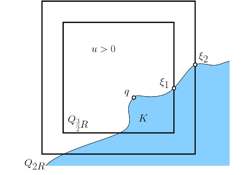
(a) Case $2b_{1}$

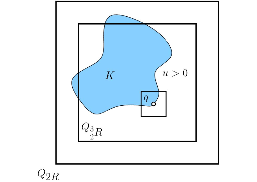
(b) Case $2b_{2}$

Figure 1. The two sub-cases of Case 2b

In Case $2b_{1}$), that is when $\partial K\cap\partial Q_{2R}\neq\emptyset$, we have that

(4.26) $$\mathcal{H}^{1}(\partial\{u^{+}_{j}=0\}\cap(Q_{2R}\setminus Q_{\frac{3}{2}R}))\geq\frac{R}{8},$$

since $u_{j}$ is a continuous functions. Indeed, let $\xi_{1}$ and $\xi_{2}$ be the intersection points of $\partial K$ with $\partial Q_{\frac{3}{2}R}$ and $\partial Q_{2R}$, respectively, and let $K_{0}$ be the orthogonal projection of $\tau:=\partial K\cap(Q_{2R}\setminus Q_{\frac{3}{2}R})$ on the line joining $\xi_{1}$ and $\xi_{2}$. We consider a covering of $\tau$, namely $\tau\subset\cup_{i\in I}B_{i}(x_{i})$, such that $\hbox{diam}B_{i}(x_{i})<\varepsilon$ for every $i\in I$. Hence, denoting by $\bar{x}_{i}$, $i\in I$, the projection of $x_{i}$ on the line that joins $\xi_{1}$ and $\xi_{2}$, we find a covering for $K_{0}$, that is $K_{0}\subset\cup_{i\in I}B_{i}(\bar{x}_{i})$, with $\hbox{diam}B_{i}(\bar{x}_{i})<\varepsilon$. Consequently,

$$\mathcal{H}^{1}_{\varepsilon}(\tau)\geq\mathcal{H}^{1}_{\varepsilon}(K_{0})=\inf\sum_{i\in I}\hbox{diam}B_{i}(\bar{x}_{i})\geq\frac{R}{8},$$

where the infimum is taken over all the coverings of $K_{0}$ such that $\hbox{diam}B_{i}(\bar{x}_{i})<\varepsilon$. Hence, sending $\varepsilon$ to zero we obtain (4.26).

We notice that (4.26) gives a lower bound of the capacity, thanks to (3.10), and so we conclude as in Case 1).

In Case $2b_{2}$), that is when $\partial K\Subset Q_{2R}$, we recall Subsection 3.2 in order to conclude that the free boundary is given just by $\partial\{u>0\}$.

That said, we observe that if $u_{j}\leq 0$ inside $K$ and $u_{j}\leq 0$ outside, then actually $u_{j}\equiv 0$ inside $K$, since $u_{j}=0$ on $\partial K$ and it is $p_{j}$-subharmonic inside. Thus

(4.27) $$u_{j}\geq 0\quad{\mbox{ in }}Q_{\frac{3}{2}R}.$$

Thus, we can consider the pure one-phase minimization problem (3.7) in $Q_{\frac{3}{2}R}$ (recall that $\Lambda>0$).

Now, if $Q_{\frac{3}{4}R}$ is contained in the set $K$, then we have a uniform lower bound for the capacity, and so we conclude as in Case 1).

Hence we suppose that $Q_{\frac{3}{4}R}$ is not contained in $K$, and we take a small square centered at $q$, say $Q_{\frac{R}{8}}(q)$, such that $Q_{\frac{R}{8}}(q)\subset Q_{\frac{3}{4}R}$ (see Figure 1(B)).

Now, recalling (4.27), we have that we can deal with a one-phase problem in the square $Q_{\frac{R}{8}}(q)$. Hence, from Theorem 4.4 in [12] we obtain that

$$|\{u_{j}^{+}=0\}\cap Q_{\frac{3}{8}R}(q)|\geq c_{0}R^{2},$$

for some universal constant $c_{0}>0$, see Figure 1(B). Again this implies a lower bound for the capacity, thanks to (3.11), and so we conclude as in Case 1).

Suppose now that there is another component $K_{2}\subset\{u^{+}_{j}=0\}$ such that $K_{2}\cap Q_{\frac{3}{2}R}\neq\emptyset$ (that is $u_{j}$ may change sign). Then, as before, either $\partial K_{2}\cap\partial Q_{2R}\neq\emptyset$ or $\partial K\Subset Q_{2R}$. In the first case, we obtain a lower bound for the capacity reasoning as in Case $2b_{1})$. In the second case, we use again the maximum principle to reduce ourselves to a one-phase minimization problem and, from the density estimate for the zero set, we get a lower bound for the capacity.

Case 3): Finally we deal with the last case, which is the easiest one. In fact the proof follows as in Case 2a) if we replace there $Q_{\frac{3R}{2}}$ with $Q_{2R}$.

Thus, since $p_{j}>2$, for any $p_{0}/2<\ell<2$ we obtain the claim in (4.12) also for squares that do not touch $\partial\{u_{j}^{+}=0\}$.

Combining all the cases treated above, we can see that for any square $Q_{2R}\subset B_{3}$ and some fixed $\ell$ with $p_{0}/2<\ell<2$ there exists a tame constant $C>0$ such that there holds

$$\left(\fint_{Q_{R}}|\nabla u^{+}_{j}|^{2}\right)^{1/2}\leq C\,\left(\fint_{Q_{2R}}|\nabla u^{+}_{j}|^{\ell}\right)^{1/\ell}.$$

Therefore we can apply the Gehring’s Lemma (see Proposition 3.6, and for instance [18] for the proof) and we get that there exists $q>2$ such that

$$\|\nabla u^{+}_{j}\|_{L^{q}(Q_{R})}\leq C,$$

for a suitable $C>0$. By a covering argument, this implies the desired result. ∎

From the uniform estimates in $W^{1,q}_{loc}(B_{3})$, with $q>2$, and the Sobolev’s embedding Theorem we immediately get the following:

Corollary 4.3.

The functions $u_{j}^{\pm}$ are uniformly continuous in $B_{2}$.

4.4. Step 3: Linearity in $B_{3}\setminus B_{1}$

Thanks to Lemma 4.2 and a standard compactness argument, we conclude that

(4.28) $$\nabla u^{\pm}_{j} L^{q^{\prime}}(B_{1}) q^{\prime}<q q>2 \nabla u_{0}^{\pm}$$ converges strongly in , for any , with , to some .

Moreover, Lemma 4.1 implies that both $u^{+}_{0}$ and $u^{-}_{j}$ are non-degenerate. Therefore, since $p_{j}\rightarrow 2$ as $j\to+\infty$, from (4.5) we deduce that

$$\liminf_{j\to\infty}\varphi_{p_{j}}(1,u_{j},0) \geq \liminf_{j\to\infty}\varphi_{p_{j}}(3,u_{j},0)$$

$$= \liminf_{j\to\infty}3^{-4}\int_{B_{3}}|\nabla u^{+}_{j}|^{p_{j}}\,\int_{B_{3}}|\nabla u^{-}_{j}|^{p_{j}}$$

$$\geq 3^{-4}\int_{B_{3}}|\nabla u^{+}_{0}|^{2}\,\int_{B_{3}}|\nabla u^{-}_{0}|^{2}\equiv\varphi_{2}(3,u_{0},0),$$

where the last line follows from the semicontinuity of the Dirichlet’s integral.

On the other hand, (4.28) implies strong convergence of the gradient in $L^{2}(B_{1})$, since $q>2$ in Lemma 4.2. Therefore

$$\liminf_{j\to\infty}\varphi_{p_{j}}(1,u_{j},0)=\liminf_{j\rightarrow+\infty}\int_{B_{1}}|\nabla u^{+}_{j}|^{p_{j}}\,\int_{B_{1}}|\nabla u^{-}_{j}|^{p_{j}}=\int_{B_{1}}|\nabla u^{+}_{0}|^{2}\,\int_{B_{1}}|\nabla u^{-}_{0}|^{2}.$$

Hence,

(4.30) $$\varphi_{2}(3,u_{0},0)\leq\int_{B_{1}}|\nabla u^{+}_{0}|^{2}\,\int_{B_{1}}|\nabla u^{-}_{0}|^{2}=\varphi_{2}(1,u_{0},0).$$

Now, we observe that $u_{0}^{+}$ and $u_{0}^{-}$ are non-negative subharmonic functions with disjoint supports fulfilling the conditions of Theorem 3.5, and so the monotonicity of $\varphi_{2}$ implies that

$$\varphi_{2}(1,u_{0},0)\leq\varphi_{2}(3,u_{0},0).$$

This and (4.30) give that $\varphi_{2}$ is constant in $B_{3}\setminus B_{1}$. Thus, Theorem 3.5 yields that $u^{+}_{0}$ and $u^{-}_{0}$ must be linear in $B_{3}\setminus B_{1}$, say, $u_{0}^{+}=\alpha x_{1}^{+}$ and $u_{0}^{-}=\beta x_{1}^{-}$, for some $\alpha$ and $\beta>0$.

4.5. Step 4: Filling in the gap

In this subsection we want to show that $u^{+}_{0}$ and $u^{-}_{0}$ are linear in $B_{3}$, and this will give a contradiction with (4.9). For this, we will prove that either $u_{0}^{+}$ in $\{u_{0}>0\}$ or $u_{0}^{-}$ in $\{u_{0}<0\}$ is harmonic, in order to employ some unique continuation result.

Let us show that

(4.31) $$u_{0}^{+} \{u_{0}>0\}$$ is harmonic in 

(the proof for $u_{0}^{-}$ is analogous). We take a point $x_{0}\in\Omega$ such that $u_{0}(x_{0})>0$, then, thanks to the uniform convergence of $u_{j}$ to $u_{0}$, we have that $u_{j}(x_{0})>0$ for $j$ large enough. Therefore, Corollary 4.3 implies that there exists a small $\delta=\delta(x_{0})>0$ such that $u_{j}>0$ in $B_{\delta}(x_{0})$, and so we can use P.1 in Proposition 3.1 to obtain that

$$\Delta_{p_{j}}u_{j}=0\quad{\mbox{ in }}B_{\delta}(x_{0}).$$

Therefore, for any $\psi\in C^{\infty}_{0}(B_{\delta}(x_{0}))$, we have that

$$\int_{B_{\delta}(x_{0})}|\nabla u_{j}|^{p_{j}}\leq\int_{B_{\delta}(x_{0})}|\nabla u_{j}+\nabla\psi|^{p_{j}}.$$

Taking the limit as $j\to+\infty$ we have that

(4.32) $$\int_{B_{\delta}(x_{0})}|\nabla u_{0}|^{2}\leq\int_{B_{\delta}(x_{0})}|\nabla u_{0}+\nabla\psi|^{2},\quad{\mbox{ for any }}\psi\in C^{\infty}_{0}(B_{\delta}(x_{0}))$$

(recall that $\varphi$ is fixed and that we have strong convergence of $\nabla u_{j}$ to $\nabla u_{0}$ in $L^{2}_{loc}(B_{3})$). By a density argument, from (4.32) we get

$$\int_{B_{\delta}(x_{0})}|\nabla u_{0}|^{2}\leq\int_{B_{\delta}(x_{0})}|\nabla v|^{2},\quad{\mbox{ for any }}v\in W^{1,2}(B_{\delta}(x_{0}))\ {\mbox{ s.t. }}v-u_{0}\in W^{1,2}(B_{\delta}(x_{0})).$$

Thus we conclude that

$$\Delta u_{0}=0\quad{\mbox{ in }}B_{\delta}(x_{0}).$$

Since $u_{0}$ is a continuous function, this implies (4.31).

From Step 3 and (4.31), and applying the Unique Continuation Theorem (see [17]), we obtain that

(4.33) $$u^{+}_{0} u^{-}_{0} B_{3}$$ and  are linear in .

On the other hand, the uniform convergence of $u_{j}$ to $u_{0}$, as $j\to+\infty$, implies that (4.9) holds true, and so the level sets of $u_{0}$ are not flat in $B_{1}$. Indeed, by the uniform convergence, for any $\varepsilon>0$ there is $j_{0}$ such that $|Cx_{1}-u_{j}^{+}(x)|<\varepsilon$ whenever $j>j_{0}$, where we assume that $u_{0}^{+}(x)=Cx_{1}$ for some constant $C>0$. Since $\partial\{{u_{j}>0}\}$ is $h_{0}$ thick in $B_{1}$ it follows that there is $y_{j}\in\partial\{{u_{j}>0}\}\cap B_{1}$ such that $y_{j}=e_{1}h_{0}/2+t_{j}e_{2}$, for some $t_{j}\in\mathbb{R}$, where $e_{1}$ is the unit direction of the $x_{1}$-axis and $e_{2}\perp e_{1}$. Then we have that $|C\frac{h_{0}}{2}-0|=|u_{0}^{+}(y_{j})-u_{j}^{+}(y_{j})|<\varepsilon$ which is in contradiction with (4.33), and thus concludes the proof of Theorem 2.1.

5. Proof of Theorem 2.2

In this section we prove Theorem 2.2. For this, we recall Corollary 3.4 and we square (3.6): we have

(5.1) $$\left(\frac{1}{r}\fint_{B_{r}(x_{0})}u^{+}\right)^{2}+\left(\frac{1}{r}\fint_{B_{r}(x_{0})}u^{-}\right)^{2}\leq C^{2}+\frac{2}{r^{2}}\fint_{B_{r}(x_{0})}u^{+}\fint_{B_{r}(x_{0})}u^{-},$$

where $C>0$ is the constant appearing in Corollary 3.4.

Now we set $u_{r}^{\pm}(x):=u^{\pm}(rx)$. So from the Hölder inequality, the Poincaré inequality (3.12) and (3.10), we have that, for any $1<\ell<2$,

$$\fint_{B_{r}(x_{0})}u^{\pm}(x)\,dx\leq\left(\fint_{B_{r}(x_{0})}(u^{\pm})^{\ell}(x)\,dx\right)^{\frac{1}{\ell}}=\left(\fint_{B_{1}(x_{0})}(u^{\pm}_{r})^{\ell}(y)\,dy\right)^{\frac{1}{\ell}}$$

$$\qquad\leq C_{1}\left(\fint_{B_{1}(x_{0})}|\nabla u^{\pm}_{r}(y)|^{\ell}\,dy\right)^{\frac{1}{\ell}}=C_{1}\left(r^{\ell}\fint_{B_{r}(x_{0})}|{\nabla}u^{\pm}|^{\ell}\right)^{\frac{1}{\ell}}$$

$$\qquad=C_{1}\,r\left(\fint_{B_{r}(x_{0})}|{\nabla}u^{\pm}|^{\ell}\right)^{\frac{1}{\ell}},$$

for some $C_{1}>0$. However, from Hölder’s inequality we have for $p>2>\ell>1$

$$\left(\fint_{B_{r}(x_{0})}|{\nabla}u^{\pm}|^{\ell}\right)^{\frac{1}{\ell}}\leq\left(\fint_{B_{r}(x_{0})}|{\nabla}u^{\pm}|^{p}\right)^{\frac{1}{p}}.$$

Therefore

$$\left(\frac{1}{r}\fint_{B_{r}(x_{0})}u^{+}\right)^{2}+\left(\frac{1}{r}\fint_{B_{r}(x_{0})}u^{-}\right)^{2}\leq C^{2}+C_{2}(\varphi_{p}(r,u,x_{0}))^{\frac{1}{p}},$$

for some $C_{2}>0$.

Let now $r_{k}:=3^{-k_{0}-k}$, for any $k\in\mathbb{N}$, where $k_{0}$ is the smallest positive integer such that $3^{-k_{0}}<r_{0}$. If $3^{-m-1}\leq r\leq 3^{-m}$, for some $m\in\mathbb{N}$, then

$$\varphi_{p}(r,u,x_{0})\leq C_{3}\varphi_{p}(3^{-m},u,x_{0})\leq C_{3}\varphi_{p}(3^{-k_{0}},u,x_{0})$$

for some $C_{3}>0$, implying that

$$\left(\frac{1}{r}\fint_{B_{r}(x_{0})}u^{\pm}\right)^{2}\leq C^{2}+C(\varphi_{p}(3^{-k_{0}},u,x_{0}))^{\frac{1}{p}},$$

for suitable $C_{4}>0$. Hence, P.4 in Proposition 3.1 and the weak maximum principle (see Corollary 3.10 in [22]) imply the estimate $\sup_{B_{r}(x_{0})}|u|\leq Cr$. This completes the proof of Theorem 2.2.

6. Viscosity solutions

In order to apply the regularity theory for free boundary problems developed for the viscosity solutions in [20, 21] we shall observe that any weak $W^{1,p}$ minimizer is also viscosity solution (see Definition 2.4 in [10] for the case $p=2$). For this, we denote by $\Omega^{+}(u):=\{u>0\}$ and $\Omega^{-}(u):=\{u<0\}$. Moreover,

$$G(u^{+}_{\nu},u^{-}_{\nu}):=(u^{+}_{\nu})^{p}-(u^{-}_{\nu})^{p}-\frac{\Lambda}{p-1}$$

is the flux balance across the free boundary, where $u^{+}_{\nu}$ and $u^{-}_{\nu}$ are the normal derivatives in the inward direction to $\Omega^{+}(u)$ and $\Omega^{-}(u)$, respectively (recall that $\Lambda=\lambda^{p}_{+}-\lambda^{p}_{-}$).

We recall the definition of viscosity solutions for the case $p\neq 2$ (see Definition 4.1 in [14]).

Definition 6.1.

Let $\Omega$ a bounded domain in $\mathbb{R}^{2}$ and let $u$ be a continuous function in $\Omega$. We say that $u$ is a viscosity solution in $\Omega$ if

• $\Delta_{p}u=0$ in $\Omega^{+}(u)$ and $\Omega^{-}(u)$,

• along the free boundary $\Gamma=\partial\{u>0\}\cup\partial\{u<0\}$, $u$ satisfies the free boundary condition, in the sense that:

  • if at $x_{0}\in\Gamma$ there exists a ball $B\subset\Omega^{+}(u)$ such that $B\cap\Gamma=\{x_{0}\}$ and

    (6.1) $$u^{+}(x)\geq\alpha\langle x-x_{0},\nu\rangle^{+}+o(|x-x_{0}|),\ {\mbox{ for }}x\in B,$$

    (6.2) $$u^{-}(x)\leq\beta\langle x-x_{0},\nu\rangle^{-}+o(|x-x_{0}|),\ {\mbox{ for }}x\in B^{c},$$

    for some $\alpha>0$ and $\beta\geq 0$, with equality along every non-tangential domain, then the free boundary condition is satisfied

    $$G(\alpha,\beta)\leq 0,$$

  • if at $x_{0}\in\Gamma$ there exists a ball $B\subset\Omega^{-}(u)$ such that $B\cap\Gamma=\{x_{0}\}$ and

    $$u^{-}(x)\geq\beta\langle x-x_{0},\nu\rangle^{-}+o(|x-x_{0}|),\ {\mbox{ for }}x\in B,$$

    $$u^{+}(x)\leq\alpha\langle x-x_{0},\nu\rangle^{+}+o(|x-x_{0}|),\ {\mbox{ for }}x\in\partial B,$$

    for some $\alpha\geq 0$ and $\beta>0$, with equality along every non-tangential domain, then

    $$G(\alpha,\beta)\geq 0.$$

With this notion of viscosity solutions, in [14] we prove the following:

Theorem 6.2.

Let $u\in W^{1,p}(\Omega)$ be a minimizer of (1.1). Then, $u$ is also a viscosity solution in the sense of Definition 6.1.

See Theorem 4.2 in [14] for the proof of Theorem 6.2.

We also recall the notion of ${\varepsilon}-$monotonicity of a viscosity solution to our free boundary problem.

Definition 6.3.

We say that $u$ is $\varepsilon-$monotone if there are a unit vector $e$ and an angle $\theta_{0}$ with $\theta_{0}>\frac{\pi}{4}$ (say) and $\varepsilon>0$ (small) such that, for every $\varepsilon^{\prime}\geq\varepsilon$,

(6.3) $$\sup_{B_{\varepsilon^{\prime}\sin\theta_{0}}(x)}u(y-\varepsilon^{\prime}e)\leq u(x).$$

We define $\Gamma(\theta_{0},e)$ the cone with axis $e$ and opening $\theta_{0}$.

Definition 6.4.

We say that $u$ is $\varepsilon-$monotone in the cone $\Gamma(\theta_{0},{\varepsilon})$ if it is $\varepsilon-$monotone in any direction $\tau\in\Gamma(\theta_{0},\varepsilon)$.

One can interpret the ${\varepsilon}-$monotonicity of $u$ as closeness of the free boundary to a Lipschitz graph with Lipschitz constant sufficiently close to $1$ if we depart from the free boundary in directions $e$ at distance ${\varepsilon}$ and higher. The exact value of the Lipschitz constant is given by $\left(\tan\frac{\theta_{0}}{2}\right)^{-1}$. Then the ellipticity propagates to the free boundary via Harnack’s inequality giving that $\Gamma$ is Lipschitz. Furthermore, Lipschitz free boundaries are, in fact, $C^{1,\alpha}$ regular.

For $p=2$ this theory was founded by L. Caffarelli, see [6, 7, 8]. Recently J. Lewis and K. Nyström proved that this theory is valid for all $p>1$, see [20, 21].

For viscosity solutions we replace the $\varepsilon-$monotonicity with slab flatness measuring the thickness of $\partial\{{u>0}\}\cap B_{r}(x)$ in terms of the quantity $h(x,r)$ introduced in (2.3). In other words, $h(x,r)$ measures how close the free boundary is to a pair of parallel planes in a ball $B_{r}(x)$ with $x\in\Gamma.$ Clearly, planes are Lipschitz graphs in the direction of the normal, therefore the slab flatness of $\Gamma$ is a particular case of ${\varepsilon}-$monotonicity of $u$.

Hence, under $h_{0}-$flatness of the free boundary we can reformulate the regularity theory “flatness implies $C^{1,\alpha}$” as follows:

Theorem 6.5.

Let $x_{0}\in\partial\{{u>0}\}$ and $r>0$ such that $B_{r}(x_{0})\subset\Omega$. Then there exists $h>0$ such that if $\Gamma\cap B_{r}(x_{0})\subset\{x\in\mathbb{R}^{N}:-hr<(x-x_{0})\cdot\nu<hr\}$ then $\Gamma\cap B_{r/2}(x_{0})$ is locally $C^{1,\alpha}$ in the direction of $\nu$, for some $\alpha\in(0,1)$.

7. Geometry of eigenvalues

Here we present some results that are related to the characteristic numbers and the eigenvalues of the $p$-Laplace-Beltrami operator for $p\neq 2$.

7.1. Homogeneous $p$-harmonic functions in complementary cones

Let us consider

$$\varphi_{p}(R,u_{1},u_{2}0):=\frac{1}{R^{4}}\int_{B_{R}}|\nabla u_{1}|^{p}\,\int_{B_{R}}|\nabla u_{2}|^{p},$$

for given $u_{i}=r^{\lambda_{i}}g_{i}(\theta)$, with $i=1,2$ such that $u_{1},u_{2}$ are $p-$harmonic in two complementary cones. Here $r,\theta$ are the polar coordinates. We will show an estimate on the eigenvalues $\lambda_{1}$ and $\lambda_{2}$ of the $p$-Laplace-Beltrami operator, namely we prove that

(7.1) $$\begin{split}&\sqrt{\lambda_{1}(\lambda_{1}(p-1)+2-p)}+\sqrt{\lambda_{2}(\lambda_{2}(p-1)+2-p)}\geq 2,\\ &{\mbox{with equality if and only if both functions are linear.}}\end{split}$$

In turn, this implies that $\varphi_{p}(R,u_{1},u_{2}0)$ is non-decreasing in $R$. Furthermore, $\varphi_{p}(R,u_{1},u_{2}0)$ is constant if and only if $\lambda_{1}=\lambda_{2}=0$.

7.2. Properties of Eigenvalues

In this section we prove a relation between the eigenvalues of the $p-$Laplace-Beltrami operator that correspond to two complementary cones. We begin with an existence result of P. Tolksdorf [23], page 780, Theorem 2.1.1 and Corollary 2.1.

Theorem 7.1.

Let $S:=(0,\omega)$, with $\omega\in[0,2\pi]$. Then there exists a solution $(\lambda,\varphi(\theta))$, with $\theta\in S$ of

(7.2) $$\left\{\begin{array}[]{ccc}-\frac{d}{d\theta}\left\{(\lambda^{2}\varphi^{2}+\varphi_{\theta}^{2})^{\frac{p-2}{2}}\varphi_{\theta}\right\}=\lambda(\lambda(p-1)+2-p)(\lambda^{2}\varphi^{2}+\varphi_{\theta}^{2})^{\frac{p-2}{2}}\varphi\ {\rm in}\ S,\\ \varphi(\theta)=0\ {\rm on}\ \partial S,\end{array}\right.$$

such that

$$\lambda>\max\left\{0,\frac{p-2}{p-1}\right\},\ \varphi>0\ {\rm in}\ S,$$

and $$\varphi^{2}+\varphi_{\theta}^{2}>0\ {\rm in}\ S.$$

Furthermore any two solutions are constant multiples of each other.

M. Dobrowolski computed explicitly the value of $\lambda$ in (7.2), see [15] page 187, Theorem 1:

Theorem 7.2.

Let $\varphi$ be given by Theorem 7.1. Then

(7.6) $$\lambda=\left\{\begin{array}[]{ccc}s+\sqrt{s^{2}+\frac{1}{\rho}},&\omega\leq\pi,\\ s-\sqrt{s^{2}+\frac{1}{\rho}},&\pi\leq\omega<2\pi,\\ \frac{p-1}{p},&\omega=2\pi,\end{array}\right.$$

where

(7.7) $$\rho := \left(\frac{\omega}{\pi}-1\right)^{2}-1,$$

(7.8) $${\mbox{and }}\;s := \frac{(\rho-1)p-2\rho}{2\rho(p-1)}=\frac{p-2}{2(p-1)}+\frac{p}{2(p-1)}\left[-\frac{1}{\rho}\right].$$

The key result of this section is contained in the following lemma.

Lemma 7.3.

Let $\lambda_{1}$ be the solution of (7.2) for $S_{1}:=(0,\omega)$ and $\lambda_{2}$ for the complementary arc $S_{2}:=(\omega,2\pi)$. Then

(7.9) $$\sqrt{\lambda_{1}(\lambda_{1}(p-1)+2-p)}+\sqrt{\lambda_{2}(\lambda_{2}(p-1)+2-p)}\geq 2.$$

Furthermore equality holds if and only if $\lambda_{1}=\lambda_{2}=1$, i.e. for half circles $S=(0,\pi)$.

Proof.

Without loss of generality we may assume that $\omega\leq\pi$. Next let us notice that the eigenvalue $\lambda$ is determined by the size of the arc only. Hence for $S_{2}$ we have by (7.7)

$$\rho_{2}=\left(\frac{2\pi-\omega}{\pi}-1\right)^{2}-1=\left(1-\frac{\omega}{\pi}\right)^{2}-1.$$

Thus $\rho_{1}=\rho_{2}=\rho$ and from (7.8) we infer that $s_{1}=s_{2}=s$. In order to prove (7.9) it is enough to check that

(7.10) $$\begin{split}&I+2\sqrt{II}\geq 4,\\ {\mbox{where }}\;&I:=\lambda_{1}(\lambda_{1}(p-1)+2-p)+\lambda_{2}(\lambda_{2}(p-1)+2-p)\\ {\mbox{and }}\;&II:=\lambda_{1}\lambda_{2}(\lambda_{1}(p-1)+2-p)(\lambda_{2}(p-1)+2-p).\end{split}$$

In order to prove this, we notice that, by (7.6),

$$\left\{\begin{array}[]{ccc}\lambda_{1}+\lambda_{2}&=&2s\\ \lambda_{1}\lambda_{2}&=&-\frac{1}{\rho}\\ \lambda_{1}^{2}+\lambda_{2}^{2}&=&4s^{2}+\frac{2}{\rho}\end{array}\right.$$

which gives

(7.12) $$I=(\lambda_{1}^{2}+\lambda_{2}^{2})(p-1)+(2-p)(\lambda_{1}+\lambda_{2})=(p-1)\left(4s^{2}+\frac{2}{\rho}\right)+2s(2-p).$$

For convenience we introduce a new quantity

(7.13) $$t:=-\frac{1}{\rho}$$

and notice that, by (7.7), we have that $t\geq 1$ and, by (7.8), one has

(7.14) $$s=\frac{1}{2(p-1)}(p-2+pt).$$

Hence (7.12) can be manipulated further in the following way:

$$I = 2\left[(p-1)\left(2s^{2}+\frac{1}{\rho}\right)+s(2-p)\right]$$

$$= 2\left[s\left\{2s(p-1)+(2-p)\right\}+(p-1)\frac{1}{\rho}\right]$$

$$= 2\left[s\left\{(p-2+pt)+(2-p)\right\}+(p-1)\frac{1}{\rho}\right]$$

$$= 2\left[spt-t(p-1)\right]$$

$$= 2t[sp-(p-1)].$$

Similarly, using (7.6) and (7.14) we get

$$II = \lambda_{1}\lambda_{2}(\lambda_{1}(p-1)+2-p)(\lambda_{2}(p-1)+2-p)$$

$$= -\frac{1}{\rho}\left[\lambda_{1}\lambda_{2}(p-1)^{2}+(p-1)(2-p)(\lambda_{1}+\lambda_{2})+(2-p)^{2}\right]$$

$$= -\frac{1}{\rho}\left[-\frac{1}{\rho}(p-1)^{2}+2s(p-1)(2-p)+(2-p)^{2}\right]$$

$$= t\left[t(p-1)^{2}+2s(p-1)(2-p)+(p-2)^{2}\right]$$

$$= t\left[t(p-1)^{2}+(p-2+pt)(2-p)+(2-p)^{2}\right]$$

$$= t\left[t(p-1)^{2}+pt(2-p)\right]$$

$$= t^{2}.$$

Thus, putting together the last two formulas,

(7.15) $$\begin{split}I+2\sqrt{II}=\,&2t[sp-(p-1)]+2t\\ =\,&2t\left[sp-(p-1)+1\right]\\ =\,&2t\left[\frac{p}{2(p-1)}(p-2+pt)-(p-1)+1\right]\\ =\,&\frac{t}{p-1}\left[p(p-2+pt)-2(p-1)(p-2)\right]\\ =\,&\frac{t}{p-1}\left[p^{2}-2p+p^{2}t-2p^{2}+6p-4)\right]\\ =\,&\frac{t}{p-1}\left[p^{2}(t-1)+4(p-1)\right]\\ =\,&4t+\frac{p^{2}}{p-1}t(t-1)\\ \geq\,&4\end{split}$$

since $t\geq 1$, which implies (7.10) and finishes the proof of Lemma 7.10. ∎

7.3. Computing the logarithmic derivative

In what follows, fixed $u_{1}$ and $u_{2}$, we put $\varphi(R):=\varphi_{p}(R,u_{1},u_{2},0)$. In order to prove that $\varphi$ is non-decreasing in $R$, it is enough to prove that $\varphi^{\prime}(R)\geq 0$ for $R=1$, since $\varphi$ is scale-invariant. For this, let $J_{i}:=\int_{B_{R}}|{\nabla}u_{i}|^{p}$. Then we have

$$\displaystyle(\log\varphi(R))^{\prime}=\frac{\varphi^{\prime}(R)}{\varphi(R)} = \frac{J^{\prime}_{1}(R)}{J_{1}(R)}+\frac{J_{2}^{\prime}(R)}{J_{2}(R)}-\frac{4}{R}$$

$$= \displaystyle\frac{\int_{\partial B_{R}}|{\nabla}u_{1}|^{p}}{\int_{B_{R}}|{\nabla}u_{1}|^{p}}+\frac{\int_{\partial B_{R}}|{\nabla}u_{2}|^{p}}{\int_{B_{R}}|{\nabla}u_{2}|^{p}}-\frac{4}{R}$$

$$= \displaystyle\frac{1}{R}\left(\frac{R\int_{\partial B_{R}}|{\nabla}u_{1}|^{p}}{\int_{B_{R}}|{\nabla}u_{1}|^{p}}+\frac{R\int_{\partial B_{R}}|{\nabla}u_{2}|^{p}}{\int_{B_{R}}|{\nabla}u_{2}|^{p}}-4\right).$$

Next we notice that

$$\int_{B_{1}}|{\nabla}u_{i}|^{p} = \int_{\partial B_{1}}|{\nabla}u_{i}|^{p-2}u_{i}\frac{\partial u_{i}}{\partial\nu}$$

$$\leq \left[\int_{\partial B_{1}}|{\nabla}u_{i}|^{p-2}u^{2}_{i}\int_{\partial B_{1}}|{\nabla}u_{i}|^{p-2}u_{i,{\rm rad}}^{2}\right]^{\frac{1}{2}},\quad i=1,2,$$

where $u_{i,\nu}=u_{i,{\rm rad}}$ is the radial derivative (in direction of the outer unit normal $\nu$ of unit circle).

Next decomposing $|{\nabla}u_{i}|^{2}$ into the sum of the squares of the radial and tangential derivative, $u_{i,\theta}$, we obtain

$$\int_{\partial B_{1}}|{\nabla}u_{i}|^{p} = \int_{\partial B_{1}}|\nabla u_{i}|^{p-2}(u_{i,{\rm rad}}^{2}+u_{i,\theta}^{2})\geq$$

$$\geq 2\left[\int_{\partial B_{1}}|{\nabla}u_{i}|^{p-2}u_{i,{\rm rad}}^{2}\int_{\partial B_{1}}|\nabla u_{i}|^{p-2}u_{i,\theta}^{2}\right]^{\frac{1}{2}}.$$

Hence to prove that $\varphi$ is monotone it is enough to check that

$$\underbrace{\left[\frac{\displaystyle\int_{S_{1}}|\nabla u_{1}|^{p-2}u_{1,\theta}^{2}}{\displaystyle\int_{S_{1}}|{\nabla}u_{1}|^{p-2}u_{1}^{2}}\right]^{\frac{1}{2}}}_{H(u_{1})}+\underbrace{\left[\frac{\displaystyle\int_{S_{2}}|\nabla u_{2}|^{p-2}u_{2,\theta}^{2}}{\displaystyle\int_{S_{2}}|{\nabla}u_{2}|^{p-2}u_{2}^{2}}\right]^{\frac{1}{2}}}_{H(u_{2})}-2\geq 0.$$

Here $S_{i}:=\operatorname{supp}u_{i}\cap\partial B_{1}$. For the solutions $(\lambda_{i},\varphi_{i})$ of the eigenvalue problem on $S_{i}$ stated in Theorem 7.1 and (7.9) we infer that $H(u_{1})+H(u_{2})\geq 2$, thanks to (7.9).

Recalling the notation in (7.10) and observing that in (7.15) the equality $I+2\sqrt{II}=4$ holds if and only if $(t-1)(4+\frac{tp^{2}}{p-1})=0$, we conclude that $t=1$. On the other hand, the equality holds in (7.9) if and only if $t=1$, i.e. by (7.13) when $\rho=-1$, and hence, in view of (7.7), when $\omega=\pi$, which corresponds to the half circle. This implies that $\varphi$ is non-decreasing, and in turn shows (LABEL:label71).

References

- [1] D.R. Adams, L.I. Hedberg: Function Spaces and Potential Theory. Springer-Verlag Berlin Heidelberg, 1999.
- [2] H. W. Alt, L. A. Caffarelli, A. Friedman: Variational problems with two phases and their free boundaries. Trans. Amer. Math. Soc. 282 (1984), no. 2, 431–461.
- [3] G. Astarita, G. Marrucci: Principles of non-Newtonian fluid mechanics. MacGraw Hill, London, New York, 1974.
- [4] G. Birkhoff, E.H. Zarantonello: Jets, Wakes, and Cavities. Academic Press, 1957.
- [5] J.E. Braga, D. Moreira: Uniform Lipschitz regularity for classes of minimizers in two phase free boundary problems i n Orlicz spaces with small density on the negative phase. Ann. Inst. H. Poincaré Anal. Non Linéaire 31 (2014), no. 4, 823–850.
- [6] L.A. Caffarelli: A Harnack inequality approach to the regularity of free boundaries. I. Lipschitz free boundaries are . Rev. Mat. Iberoamericana 3 (1987), no. 2, 139–162.
- [7] L.A. Caffarelli: A Harnack inequality approach to the regularity of free boundaries. III. Existence theory, compactness, and dependence on . Ann. Scuola Norm. Sup. Pisa Cl. Sci. (4) 15 (1988), no. 4, 583–602.
- [8] L.A. Caffarelli: A Harnack inequality approach to the regularity of free boundaries. II. Flat free boundaries are Lipschitz. Comm. Pure Appl. Math. 42 (1989), no. 1, 55–78.
- [9] L.A. Caffarelli, L. Karp, H. Shahgholian: Regularity of a free boundary with application to the Pompeiu problem. Ann. of Math. (2) 151 (2000), no. 1, 269–292.
- [10] L.A. Caffarelli, S. Salsa: A geometric approach to free boundary problems. Graduate Studies in Mathematics, 68. American Mathematical Society, Providence, RI, 2005. x+270 pp.
- [11] A. Cianchi: Continuity properties of functions from Orlicz-Sobolev spaces and embedding theorems. Ann. Scuola Norm. Sup. Pisa Cl. Sci. (4) 23 (1996), no. 3, 575–608.
- [12] D. Danielli, A. Petrosyan: A minimum problem with free boundary for a degenerate quasilinear operator. Calc. Var. Partial Differential Equations 23 (2005), no. 1, 97–124.
- [13] E. DiBenedetto, J. Manfredi, On the higher integrability of the gradient of weak solutions of certain degenerate elliptic systems. Amer. J. Math. 115 (1993), no. 5, 1107–1134.
- [14] S. Dipierro, A.L. Karakhanyan: Stratification of free boundary points for a two-phase variational problem. Preprint (2015), http://arxiv.org/abs/1508.07447.
- [15] M. Dobrowolski: On quasilinear elliptic equations in domains with conical boundary points. J. Reine Angew. Math. 394 (1989), 186–195.
- [16] J. Frehse: Capacity methods in the theory of partial differential equations. Jahresber. Deutsch. Math.-Verein. 84 (1982), no. 1, 1–44.
- [17] N. Garofalo, F.-H. Lin: Unique continuation for elliptic operators: a geometric-variational approach. Comm. Pure Appl. Math. 40 (1987), no. 3, 347–366.
- [18] M. Giaquinta: Multiple integrals in calculus of variations and nonlinear elliptic systems. Annals of Mathematics Studies, 105. Princeton University Press, Princeton, NJ, 1983. vii+297 pp.
- [19] A.L. Karakhanyan: On the Lipschitz regularity of solutions of minimum problem with free boundary. Interfaces Free Bound. 10 (2008), no. 1, 79–86.
- [20] J. L. Lewis, K. Nyström: Regularity of Lipschitz free boundaries in two-phase problems for the -Laplace operator. Adv. Math. 225 (2010), 2565–2597.
- [21] J. L. Lewis, K. Nyström: Regularity of flat free boundaries in two-phase problems for the -Laplace operator. Ann. Inst. H. Poincaré Anal. Non Linéaire 29 (2012), 83–108.
- [22] J. Malý, W.P. Ziemer: Fine regularity of solutions of elliptic partial differential equations. Mathematical Surveys and Monographs, 51. American Mathematical Society, Providence, RI, 1997. xiv+291 pp.
- [23] P. Tolksdorf: On the Dirichlet problem for quasilinear equations in domains with conical boundary points. Comm. Partial Differential Equations 8 (1983), no. 7, 773–817.