An N-barrier maximum principle for elliptic systems arising from the study of traveling waves in reaction-diffusion systems

Abstract

By employing the N-barrier method developed in the paper, we establish a new N-barrier maximum principle for diffusive Lotka-Volterra systems of two competing species. As an application of this maximum principle, we show under certain conditions, the existence and nonexistence of traveling waves solutions for systems of three competing species. In addition, new $(1,0,0)$-$(u^{\ast},v^{\ast},0)$ waves are given in terms of the tanh function provided that the parameters satisfy certain conditions.

1 Introduction

Species diversity refers to the number of different species and abundance of each species that live within an ecological system. To be more specific, species diversity takes into consideration species richness and species evenness; the former is defined as the total number of different species and the latter the variation of abundance in individuals per species. The importance of species diversity to an ecological system lies in the fact that the ecological system with a greater species diversity may function more efficiently and productively since more resources available for other species within the ecological system will be made. Therefore, the study of species diversity has been extensively investigated via both field research and theoretical approaches.

As a suggestive example of species diversity, we investigate the situation where one exotic competing species (say, $W$) invades the ecological system of two native species (say, U and V) that are competing in the absence of $W$. Then a problem related to competitive exclusion ([2], [17], [18], [20], [28], [34]) or competitor-mediated coexistence ([5], [23], [29]) arises, and a mathematical model for this situation can be provided by the diffusive Lotka-Volterra system of three competing species ([1], [10], [12], [13], [14], [25], [27], [29], [30], [35], [38])

$$\begin{cases}\vspace{3mm}u_{t}=d_{1}\,u_{yy}+u\,(\sigma_{1}-c_{11}\,u-c_{12}\,v-c_{13}\,w),\quad y\in\mathbb{R},\quad t>0,\\ \vspace{3mm}v_{t}=d_{2}\,v_{yy}+v\,(\sigma_{2}-c_{21}\,u-c_{22}\,v-c_{23}\,w),\quad y\in\mathbb{R},\quad t>0,\\ w_{t}=d_{3}\,w_{yy}+w\,(\sigma_{3}-c_{31}\,u-c_{32}\,v-c_{33}\,w),\quad y\in\mathbb{R},\quad t>0,\end{cases}$$ (1.1)

where $u(y,t)$, $v(y,t)$ and $w(y,t)$ denote the population densities of $U$, $V$ and $W$ at time $t$ and position $y$. The parameters $d_{i}$, $\sigma_{i}$, $c_{ii}$ $(i=1,2,3)$, and $c_{ij}$ $(i,j=1,2,3\ \text{with}\;i\neq j)$, which are all positive constants, stand for the diffusion rates, intrinsic growth rates, intra-specific competition rates, and inter-specific competition rates, respectively. In particular, the result in [7] indicates from the viewpoint of competitor-mediated coexistence, the coexistence of strongly competing species in the presence of an exotic competing species.

We begin with a two-species system of (1.1) in the absence of $W$, i.e.

$$\begin{cases}u_{t}=d_{1}\,u_{yy}+u\,(\sigma_{1}-c_{11}\,u-c_{12}\,v),\quad y\in\mathbb{R},\quad t>0,\\ \\ \hskip 1.99168ptv_{t}=d_{2}\,v_{yy}+v\,(\sigma_{2}-c_{21}\,u-c_{22}\,v),\quad y\in\mathbb{R},\quad t>0.\\ \end{cases}$$ (1.2)

Imposing the zero Neumann boundary conditions

$$\frac{\partial u}{\partial\nu}=\frac{\partial v}{\partial\nu}=0,\quad x\in\partial\Omega$$ (1.3)

and suitable initial conditions

$$u(x,0)=\hat{u}(x),\;v(x,0)=\hat{v}(x),\quad x\in\Omega$$ (1.4)

on (1.2) with the entire space $\mathbb{R}$ is replaced by a bounded and convex domain $\Omega$, we conclude from [15] and [24] that any positive solution $(u(x,t),v(x,t))$ of such a initial-boundary value problem converges to either $(\frac{\sigma_{1}}{c_{11}},0)$ or $(0,\frac{\sigma_{2}}{c_{22}})$ when $U$ and $V$ are strongly competing, i.e. when the following condition hold:

$$\frac{\sigma_{1}}{c_{11}}>\frac{\sigma_{2}}{c_{21}},\,\frac{\sigma_{2}}{c_{22}}>\frac{\sigma_{1}}{c_{12}}.$$ (1.5)

In this case, Gause’s principle of competitive exclusion occurs between the two species $U$ and $V$ when $U$ and $V$ competing for the same limited resources cannot stably coexist; one will prevail and the other is excluded. When the influence of diffusion in (1.2) is disregarded, (1.2) becomes

$$\begin{cases}u_{t}=u\,(\sigma_{1}-c_{11}\,u-c_{12}\,v),\quad t>0,\\ \\ \hskip 1.99168ptv_{t}=v\,(\sigma_{2}-c_{21}\,u-c_{22}\,v),\quad t>0.\\ \end{cases}$$ (1.6)

It is readily seen that (1.6) has four equilibria: $\textbf{e}_{1}=(0,0)$, $\textbf{e}_{2}=\big{(}\frac{\sigma_{1}}{c_{11}},0\big{)}$, $\textbf{e}_{3}=\big{(}0,\frac{\sigma_{2}}{c_{22}}\big{)}$ and $\textbf{e}_{4}=(u^{\ast},v^{\ast})$, where $(u^{\ast},v^{\ast})=\big{(}\frac{c_{22}\,\sigma_{1}-c_{12}\,\sigma_{2}}{c_{11}\,c_{22}-c_{12}\,c_{21}},\frac{c_{11}\,\sigma_{2}-c_{21}\,\sigma_{1}}{c_{11}\,c_{22}-c_{12}\,c_{21}}\big{)}$ is the intersection of the two straight lines $\sigma_{1}-c_{11}\,u-c_{12}\,v=0$ and $\sigma_{2}-c_{21}\,u-c_{22}\,v=0$, whenever it exists. In the diffusion-free case, we can classify the asymptotic behaviour of solutions $(u(t),v(t))$ for (1.6) as $t\rightarrow\infty$ depending on $\sigma_{i}$ and $c_{ij}$ $(i,j=1,2)$, as described in:

Proposition 1.1 ([9]).

Suppose that $(u(t),v(t))$ is a solution of (1.6) with initial conditions $u(0),v(0)>0$. We have

• (Competitive exclusion) if $\frac{\sigma_{1}}{c_{11}}>\frac{\sigma_{2}}{c_{21}}$ and $\frac{\sigma_{2}}{c_{22}}<\frac{\sigma_{1}}{c_{12}}$, then $\lim\limits_{t\rightarrow\infty}(u(t),v(t))=\big{(}\frac{\sigma_{1}}{c_{11}},0\big{)}$;

• (Competitive exclusion) if $\frac{\sigma_{1}}{c_{11}}<\frac{\sigma_{2}}{c_{21}}$ and $\frac{\sigma_{2}}{c_{22}}>\frac{\sigma_{1}}{c_{12}}$, then $\lim\limits_{t\rightarrow\infty}(u(t),v(t))=\big{(}0,\frac{\sigma_{2}}{c_{22}}\big{)}$;

• (Strong competition) if $\frac{\sigma_{1}}{c_{11}}>\frac{\sigma_{2}}{c_{21}}$ and $\frac{\sigma_{2}}{c_{22}}>\frac{\sigma_{1}}{c_{12}}$, then $\lim\limits_{t\rightarrow\infty}(u(t),v(t))=\big{(}\frac{\sigma_{1}}{c_{11}},0\big{)}$ or $\big{(}0,\frac{\sigma_{2}}{c_{22}}\big{)}$ depending on the initial condition;

• (Weak competition) if $\frac{\sigma_{1}}{c_{11}}<\frac{\sigma_{2}}{c_{21}}$ and $\frac{\sigma_{2}}{c_{22}}<\frac{\sigma_{1}}{c_{12}}$, then $\lim\limits_{t\rightarrow\infty}(u(t),v(t))=(u^{\ast},v^{\ast})$.

As in case $(iii)$ mentioned previously, Gause’s principle of competitive exclusion also occurs in cases $(i)$ and $(ii)$: one species always wins and the other species become extinct in the long run. It is easy to see that we do not need to treat one of cases $(i)$ and $(ii)$ since one of the two cases is obtained from the other by exchanging the roles of $u$ and $v$. For the case of weak competition, the Lotka-Volterra model (1.6) predicts that the stable coexistence state $(u^{\ast},v^{\ast})$ exists only when intra-specific competition has a greater effect than inter-specific competition.

We shall assume throughout, unless otherwise stated, that either strong or weak competition occurs between the two species $U$ and $V$:

• (Strong competition) $\mathbf{[S]}$: $\frac{\sigma_{1}}{c_{11}}>\frac{\sigma_{2}}{c_{21}}$ and $\frac{\sigma_{2}}{c_{22}}>\frac{\sigma_{1}}{c_{12}}$;

• (Weak competition) $\mathbf{[W]}$: $\frac{\sigma_{1}}{c_{11}}<\frac{\sigma_{2}}{c_{21}}$ and $\frac{\sigma_{2}}{c_{22}}<\frac{\sigma_{1}}{c_{12}}$

in investigating traveling wave solutions ([36])

$$(u(y,t),v(y,t))=(u(x),v(x)),\quad x=y-\theta\,t$$ (1.7)

of (1.2). Here $\theta$ is the propagation speed of the traveling wave. We note that $u^{\ast},v^{\ast}>0$ if and only if either $\mathbf{[S]}$ or $\mathbf{[W]}$ holds. Substituting (1.7) into (1.2) yields the following system of ordinary differential equations

$$\begin{cases}d_{1}\,u_{xx}+\theta\,u_{x}+u\,(\sigma_{1}-c_{11}\,u-c_{12}\,v)=0,\quad x\in\mathbb{R},\\ \\ d_{2}\,v_{xx}\hskip 2.27621pt+\theta\,v_{x}+v\,(\sigma_{2}-c_{21}\,u-c_{22}\,v)=0,\quad x\in\mathbb{R}.\\ \end{cases}$$ (1.8)

The problem as to which species will survive in a competitive system is of importance in ecology. In order to tackle this problem, we use traveling wave solutions of the form (1.7).

In this paper, we treat the following boundary value problem

$$\begin{cases}\vspace{3mm}d_{1}\,u_{xx}+\theta\,u_{x}+u\,(\sigma_{1}-c_{11}\,u-c_{12}\,v)=0,\quad x\in\mathbb{R},\\ \vspace{3mm}d_{2}\,v_{xx}\hskip 2.27621pt+\theta\,v_{x}+v\,(\sigma_{2}-c_{21}\,u-c_{22}\,v)=0,\quad x\in\mathbb{R},\\ (u,v)(-\infty)=\text{\bf e}_{2},\quad(u,v)(+\infty)=\text{\bf e}_{4}.\end{cases}$$ (1.9)

and call a solution $(u(x),v(x))$ of (1.9) an $(\textbf{e}_{2},\textbf{e}_{4})$-wave.

Under various parameters, monotone $(\textbf{e}_{2},\textbf{e}_{4})$-waves are investigated via different approaches (for instance, [16], [21], [22]). It is not clear from the assumptions of parameters given in the references above that the monotone $(\textbf{e}_{2},\textbf{e}_{4})$-waves have the property $u^{\ast}>v^{\ast}$ or not. Let us see what happens when the answer is affirmative. If $u^{\ast}>v^{\ast}$ holds, then we easily see that, since $v$ is monotonically increasing and $u$ is monotonically decreasing the profile of $u$ lies completely above the profile of $v$. Accordingly, in this case $u$ dominates the entire habitat $\mathbb{R}$. Indeed, it has been proved that there exist two types of $(\textbf{e}_{2},\textbf{e}_{4})$-waves, one with $u^{\ast}>v^{\ast}$ and the other with $u^{\ast}\leq v^{\ast}$, by giving exact $(\textbf{e}_{2},\textbf{e}_{4})$-waves in [19]. We note that in the case $u^{\ast}>v^{\ast}$, the phenomenon exhibited by the dominance of $u$ in the entire habitat $\mathbb{R}$ is unique and is yet to be explored. In particular, exact $(\textbf{e}_{1},\textbf{e}_{2})$-waves, $(\textbf{e}_{1},\textbf{e}_{4})$-waves, $(\textbf{e}_{2},\textbf{e}_{3})$-waves and $(\textbf{e}_{2},\textbf{e}_{4})$-waves are given in [19] under certain conditions on the parameters by applying judicious ansätzes for exact solutions.

When the inhabitant of the two competing species $U$ and $V$ is resource-limited, the investigation of the total mass or the total density of the two species $U$ and $V$ is essential. This gives rises to the problem as to the estimate of the total density $u(x)+v(x)$ in (1.9). In addition, another issue which motivates us to study the estimate of $u(x)+v(x)$ is the measurement of the species evenness index $\mathcal{J}$ for (1.9). As $\mathcal{J}$ is defined via the Shannon’s diversity index $\mathcal{H}$ ([3], [11], [31], [33]), i.e.

$$\mathcal{J}=\frac{\mathcal{H}}{\ln(s)},$$ (1.10)

where

$$\mathcal{H}=-\sum_{i=1}^{s}p_{i}\cdot\ln(p_{i}),$$ (1.11)

$s$ is the total number of species, and $p_{i}$ is the proportion of the $i$-th species determined by dividing the number of the $i$-th species species by the total number of all species, the species evenness index $\mathcal{J}$ for (1.9) is given by

$$\mathcal{J}=-\frac{1}{(\ln 2)(u+v)}\,\left(u\,\ln\Big{(}\frac{u}{u+v}\Big{)}+v\,\ln\Big{(}\frac{v}{u+v}\Big{)}\right).$$ (1.12)

One of our primary goals in this paper is to address the problem of giving a priori estimates of $u(x)+v(x)$, which is involved in the calculation of $\mathcal{J}$ in (1.12). On the other hand, we also are concerned with the following question when a priori estimates of $u(x)+v(x)$ are given:

Q1: How does the estimate of $u(x)+v(x)$ depend on the parameters in (1.9)?

In [6], upper and lower bounds of $u(x)+v(x)$ are given when the two diffusion rates $d_{1}$ and $d_{2}$ are equal. However, the approach employed in [6] to obtain upper or lower bounds for $u+v$ cannot be applied directly to the case where the diffusion rates $d_{1}$ and $d_{2}$ are not equal.

Q2: In (1.9), when $d_{1}\neq d_{2}$, can upper and lower bounds of $u+v$ be obtained?

As for the answer to Q2, it seems as far as we know, not available in the literature. To give an affirmative answer to this question, we develop a new but elementary approach. Moreover, employing this approach leads to a affirmative answer to the following question which is more general than Q2:

Q3: In (1.9), when $d_{1}\neq d_{2}$, can upper and lower bounds of $\alpha\,u+\beta\,v$, where $\alpha,\beta>0$ are arbitrary constants, be given?

By adding the two equations in (1.9), we obtain an equation involving $p(x)=\alpha\,u(x)+\beta\,v(x)$ and $q(x)=d_{1}\,\alpha\,u(x)+d_{2}\,\beta\,v(x)$, i.e.

$$0 =\alpha\,\big{(}d_{1}\,u_{xx}+\theta\,u_{x}+u\,(\sigma_{1}-c_{11}\,u-c_{12}\,v)\big{)}+\beta\,\big{(}d_{2}\,v_{xx}+\theta\,v_{x}+v\,(\sigma_{2}-c_{21}\,u-c_{22}\,v)\big{)}$$

$$=q^{\prime\prime}(x)+\theta\,p^{\prime}(x)+\alpha\,u\,(\sigma_{1}-c_{11}\,u-c_{12}\,v)+\beta\,v\,(\sigma_{2}-c_{21}\,u-c_{22}\,v)$$

$$=q^{\prime\prime}(x)+\theta\,p^{\prime}(x)+F(u,v).$$ (1.13)

For the sake of clear exposition we shall assume from now on that $F(u,v)=\alpha\,u\,(\sigma_{1}-c_{11}\,u-c_{12}\,v)+\beta\,v\,(\sigma_{2}-c_{21}\,u-c_{22}\,v)$. The case where $d_{1}=d_{2}$ or $p(x)$ is a non-zero constant multiple of $q(x)$ has been considered in [6]. A mathematical difficulty arises as a consequence of the fact that the approach used in [6] cannot be directly applied, when $d_{1}\neq d_{2}$ in the last equation since $p(x)$ no long can be written as a constant multiple of $q(x)$ and such $p(x)$ and $q(x)$ are involved in a single equation like (1). The approach proposed here can be employed to give estimates of $p(x)$ in the case where $p(x)$ and $q(x)$ are involved in the single equation (1). One of the main results of this paper is the N-barrier maximum principle (Theorem 2.1), which gives an affirmative answer to Q3.

The rest of the paper is organized as follows. In the next section, the main results of this paper, including the N-barrier maximum principle (Theorem 2.1) and two applications (Theorem 2.2 and Theorem 2.3) to the system of three species (1.1), are summarized. We prove in Section 3 the N-barrier maximum principle by means of the construction of N-barriers depending on various conditions. Under certain restrictions on the parameters, the existence of exact traveling waves solutions for (1.1) (Theorem 4.1) is presented in Section 4. Finally, Section 5 is devoted to the proofs of Theorem 2.2 and Theorem 2.3.

2 Statement of main theorems

Theorem 2.1 (N-barrier maximum principle).

Under either $\mathbf{[S]}$ or $\mathbf{[W]}$, we assume that $(u(x),v(x))$ with $u(x),v(x)>0$ for $x\in\mathbb{R}$ satisfies the boundary value problem (1.9). For any $\alpha,\beta>0$, we have

$$q_{\ast}\leq\alpha\,u(x)+\beta\,v(x)\leq q^{\ast},\quad x\in\mathbb{R},$$ (2.1)

where

$$q_{\ast}=\min\bigg{[}\alpha\,\min\Big{[}\frac{\sigma_{1}}{c_{11}},\frac{\sigma_{2}}{c_{21}}\Big{]},\beta\,\min\Big{[}\frac{\sigma_{2}}{c_{22}},\frac{\sigma_{1}}{c_{12}}\Big{]}\bigg{]}\min\Big{[}\frac{d_{1}}{d_{2}},\frac{d_{2}}{d_{1}}\Big{]}$$ (2.2)

and

$$q^{\ast}=\max\bigg{[}\alpha\,\max\Big{[}\frac{\sigma_{1}}{c_{11}},\frac{\sigma_{2}}{c_{21}}\Big{]},\beta\,\max\Big{[}\frac{\sigma_{2}}{c_{22}},\frac{\sigma_{1}}{c_{12}}\Big{]}\bigg{]}\max\Big{[}\frac{d_{1}}{d_{2}},\frac{d_{2}}{d_{1}}\Big{]}.$$ (2.3)

In particular,

• (Lower bounds for $q=q(x)$) when the differential equations in (1.9) are replaced by the differential inequalities

  $$\begin{cases}\vspace{3mm}d_{1}\,u_{xx}+\theta\,u_{x}+u\,(\sigma_{1}-c_{11}\,u-c_{12}\,v)\leq 0,\quad x\in\mathbb{R},\\ d_{2}\,v_{xx}\hskip 2.27621pt+\theta\,v_{x}+v\,(\sigma_{2}-c_{21}\,u-c_{22}\,v)\leq 0,\quad x\in\mathbb{R},\\ \end{cases}$$ (2.4)

  we have $\alpha\,u(x)+\beta\,v(x)\geq q_{\ast}$ for $x\in\mathbb{R}$;

• (Upper bounds for $q=q(x)$) when the differential equations in (1.9) are replaced by the differential inequalities

  $$\begin{cases}\vspace{3mm}d_{1}\,u_{xx}+\theta\,u_{x}+u\,(\sigma_{1}-c_{11}\,u-c_{12}\,v)\geq 0,\quad x\in\mathbb{R},\\ d_{2}\,v_{xx}\hskip 2.27621pt+\theta\,v_{x}+v\,(\sigma_{2}-c_{21}\,u-c_{22}\,v)\geq 0,\quad x\in\mathbb{R},\\ \end{cases}$$ (2.5)

  we have $\alpha\,u(x)+\beta\,v(x)\leq q^{\ast}$ for $x\in\mathbb{R}$.

We would like to add a few remarks concerning Theorem 2.1.

• In addition to the diffusion rates $d_{1}$ and $d_{2}$, upper and lower bounds $q^{\ast}$ and $q_{\ast}$ depend only on the $u$-intersection (i.e. $\frac{\sigma_{1}}{c_{11}}$) of the line $\sigma_{1}-c_{11}\,u-c_{12}\,v=0$ and $v$-intersection (i.e. $\frac{\sigma_{2}}{c_{22}}$) of the line $\sigma_{2}-c_{21}\,u-c_{22}\,v=0$ as well as the $v$-intersection (i.e. $\frac{\sigma_{1}}{c_{12}}$) of the line $\sigma_{1}-c_{11}\,u-c_{12}\,v=0$ and $u$-intersection (i.e. $\frac{\sigma_{2}}{c_{21}}$) of the line $\sigma_{2}-c_{21}\,u-c_{22}\,v=0$, respectively. We note that $\textbf{e}_{2}=(\frac{\sigma_{1}}{c_{11}},0)$ and $\textbf{e}_{3}=(0,\frac{\sigma_{2}}{c_{22}})$ represent the two competitively exclusive states. When $\alpha=\beta=1$, the above observation together with the fact that the estimate of $\alpha\,u(x)+\beta\,v(x)$ given in Theorem 2.1 does not explicitly depend on the propagating speed $\theta$ gives a possible answer to Q1.

• Letting $\alpha=1$ and $\beta\rightarrow 0$ in Theorem 2.1, we obtain

  $$0\leq u(x)\leq\max\Big{[}\frac{\sigma_{1}}{c_{11}},\frac{\sigma_{2}}{c_{21}}\Big{]}\max\Big{[}\frac{d_{1}}{d_{2}},\frac{d_{2}}{d_{1}}\Big{]}.$$ (2.6)

  Letting $\beta=1$ and $\alpha\rightarrow 0$ in Theorem 2.1, we obtain

  $$0\leq v(x)\leq\max\Big{[}\frac{\sigma_{2}}{c_{22}},\frac{\sigma_{1}}{c_{12}}\Big{]}\max\Big{[}\frac{d_{1}}{d_{2}},\frac{d_{2}}{d_{1}}\Big{]}.$$ (2.7)

• When $\mathbf{[S]}$: $\frac{\sigma_{1}}{c_{11}}>\frac{\sigma_{2}}{c_{21}}$ and $\frac{\sigma_{2}}{c_{22}}>\frac{\sigma_{1}}{c_{12}}$ holds, $q^{\ast}$ and $q_{\ast}$ are given by

  $$q_{\ast}=\min\bigg{[}\alpha\,\frac{\sigma_{2}}{c_{21}},\beta\,\frac{\sigma_{1}}{c_{12}}\bigg{]}\min\Big{[}\frac{d_{1}}{d_{2}},\frac{d_{2}}{d_{1}}\Big{]}$$ (2.8)

  and

  $$q^{\ast}=\max\bigg{[}\alpha\,\frac{\sigma_{1}}{c_{11}},\beta\,\frac{\sigma_{2}}{c_{22}}\bigg{]}\max\Big{[}\frac{d_{1}}{d_{2}},\frac{d_{2}}{d_{1}}\Big{]}.$$ (2.9)

  When $\mathbf{[W]}$: $\frac{\sigma_{1}}{c_{11}}<\frac{\sigma_{2}}{c_{21}}$ and $\frac{\sigma_{2}}{c_{22}}<\frac{\sigma_{1}}{c_{12}}$ holds, $q^{\ast}$ and $q_{\ast}$ are given by

  $$q_{\ast}=\min\bigg{[}\alpha\,\frac{\sigma_{1}}{c_{11}},\beta\,\frac{\sigma_{2}}{c_{22}}\bigg{]}\min\Big{[}\frac{d_{1}}{d_{2}},\frac{d_{2}}{d_{1}}\Big{]}$$ (2.10)

  and

  $$q^{\ast}=\max\bigg{[}\alpha\,\frac{\sigma_{2}}{c_{21}},\beta\,\frac{\sigma_{1}}{c_{12}}\bigg{]}\max\Big{[}\frac{d_{1}}{d_{2}},\frac{d_{2}}{d_{1}}\Big{]}.$$ (2.11)

• By letting $\alpha=\beta=1$, we have

  $$q_{\ast}\leq u(x)+v(x)\leq q^{\ast},\quad x\in\mathbb{R},$$ (2.12)

  where

  $$q_{\ast}=\min\bigg{[}\min\Big{[}\frac{\sigma_{1}}{c_{11}},\frac{\sigma_{2}}{c_{21}}\Big{]},\min\Big{[}\frac{\sigma_{2}}{c_{22}},\frac{\sigma_{1}}{c_{12}}\Big{]}\bigg{]}\min\Big{[}\frac{d_{1}}{d_{2}},\frac{d_{2}}{d_{1}}\Big{]}$$ (2.13)

  and

  $$q^{\ast}=\max\bigg{[}\max\Big{[}\frac{\sigma_{1}}{c_{11}},\frac{\sigma_{2}}{c_{21}}\Big{]},\max\Big{[}\frac{\sigma_{2}}{c_{22}},\frac{\sigma_{1}}{c_{12}}\Big{]}\bigg{]}\max\Big{[}\frac{d_{1}}{d_{2}},\frac{d_{2}}{d_{1}}\Big{]}.$$ (2.14)

  This answers Q2.

Let us return to the system of three species (1.1) and consider traveling wave solutions

$$(u(y,t),v(y,t),w(y,t))=(u(x),v(x),w(x)),\quad x=y-\theta\,t$$ (2.15)

satisfying the following boundary value problem

$$\begin{cases}\vspace{3mm}d_{1}\,u_{xx}+\theta\,u_{x}+u\,(\sigma_{1}-c_{11}\,u-c_{12}\,v-c_{13}\,w)=0,\quad x\in\mathbb{R},\\ \vspace{3mm}d_{2}\,v_{xx}+\theta\,v_{x}+v\,(\sigma_{2}-c_{21}\,u-c_{22}\,v-c_{23}\,w)=0,\quad x\in\mathbb{R},\\ \vspace{3mm}d_{3}\,w_{xx}+\theta\,w_{x}+w\,(\sigma_{3}-c_{31}\,u-c_{32}\,v-c_{33}\,w)=0,\quad x\in\mathbb{R},\\ (u,v,w)(-\infty)=(\frac{\sigma_{1}}{c_{11}},0,0),\quad(u,v,w)(\infty)=(u^{\ast},v^{\ast},0).\end{cases}$$ (2.16)

Here again $\theta$ is the propagation speed of the traveling wave. As mentioned in the beginning of introduction, we will study the influence of an exotic species $W$ on other native species $U$ and $V$ in terms of (2.16). The first question we shall ask is whether competitor-mediated coexistence occurs for $u$, $v$, and $w$ in the system (2.16). If the three species do coexist under certain conditions, then what will be the profiles of $u(x)$, $v(x)$, and $w(x)$? The result in [19] indicates that when $w(x)$ is absent in (2.16), the system of two species (1.9) under certain conditions admits solutions $(u(x),v(x))$ having the profiles with $u(x)$ being monotonically decreasing and $v(x)$ being monotonically increasing. Moreover, we see from the profiles of $u(x)$ and $v(x)$ that $u(x)$ and $v(x)$ dominate the neighborhood of $x=-\infty$ and the neighborhood of $x=\infty$, respectively. These facts lead us to the expectation that, the profile of $w(x)$ must be pulse-like ($w(x)$ is a pulse if $w(-\infty)=w(\infty)=0$ and $w(x)>0$ for $x\in\mathbb{R}$) if it exists since $w$ will prevail only when $u$ and $v$ are not dominant.

To simplify the problem, we restrict ourself to the case of $\sigma_{1}=c_{11}$ in Section 4 and denote a solution of (2.16) with $\sigma_{1}=c_{11}$ by $(1,0,0)$-$(u^{\ast},v^{\ast},0)$ wave for convenience. Although we can find exact $(1,0,0)$-$(u^{\ast},v^{\ast},0)$ waves for (2.16) (See Theorem 4.1 and we remark that when $\sigma_{1}\neq c_{11}$, a similar result remains valid.) under certain restrictions on the parameters, it remains an open problem, however, to establish the existence of solutions for (2.16) under more general conditions. In spite of this fact, when we consider the situation where the influence of the invading species $W$ on the native species $U$ and $V$ is of no significance, i.e. $c_{13},c_{23}\approx 0$ in (2.16), the limiting case $c_{13},c_{23}\rightarrow 0^{+}$ leads to the boundary value problem

$$\begin{cases}\vspace{3mm}d_{1}\,u_{xx}+\theta\,u_{x}+u\,(\sigma_{1}-c_{11}\,u-c_{12}\,v)=0,\quad x\in\mathbb{R},\\ \vspace{3mm}d_{2}\,v_{xx}+\theta\,v_{x}+v\,(\sigma_{2}-c_{21}\,u-c_{22}\,v)=0,\quad x\in\mathbb{R},\\ \vspace{3mm}d_{3}\,w_{xx}+\theta\,w_{x}+w\,(\sigma_{3}-c_{31}\,u-c_{32}\,v-c_{33}\,w)=0,\quad x\in\mathbb{R},\\ (u,v,w)(-\infty)=(\frac{\sigma_{1}}{c_{11}},0,0),\quad(u,v,w)(\infty)=(u^{\ast},v^{\ast},0).\end{cases}$$ (2.17)

Under the assumption of the existence of solutions $(u(x),v(x))=(\tilde{u}(x),\tilde{v}(x))$ for the system of two species (1.9) ([16], [19], [21], [22]), it will be proved in Section 5.1 that under certain conditions, a solution $w(x)$ of the third equation in (2.17), i.e. the non-autonomous Fisher equation for $w=w(x)$

$$d_{3}\,w_{xx}+\theta\,w_{x}+w\,(\sigma_{3}-c_{31}\,\tilde{u}-c_{32}\,\tilde{v}-c_{33}\,w)=0,\quad x\in\mathbb{R}$$ (2.18)

can be found applying the supersolution-subsolution method, thereby establishing the existence of solutions for (2.17). We remark that, as an application of the N-barrier maximum principle, upper and lower bounds of $c_{31}\,\tilde{u}+c_{32}\,\tilde{v}$ are used in constructing supersolutions and subsolutions of (2.18).

Theorem 2.2 (Existence of traveling wave solutions for three competing species).

Assume either $\mathbf{[S]}$ or $\mathbf{[W]}$. Suppose that there exist $u=\tilde{u}(x)$ and $v=\tilde{v}(x)$ which solve the first two equations in (2.17) for some $\theta$, $d_{i}$, $\sigma_{i}$, $c_{ii}$ $(i=1,2)$, and $c_{ij}$ $(i,j=1,2\ \text{with}\;i\neq j)$ and satisfy the boundary conditions $(u,v)(-\infty)=(1,0),(u,v)(\infty)=(u^{\ast},v^{\ast})$. Let

$$\underaccent{\bar}{q}=\min\bigg{[}c_{31}\min\Big{[}\frac{\sigma_{1}}{c_{11}},\frac{\sigma_{2}}{c_{21}}\Big{]},c_{32}\min\Big{[}\frac{\sigma_{2}}{c_{22}},\frac{\sigma_{1}}{c_{12}}\Big{]}\bigg{]}\min\Big{[}\frac{d_{1}}{d_{2}},\frac{d_{2}}{d_{1}}\Big{]}$$ (2.19)

and

$$\bar{q}=\max\bigg{[}c_{31}\max\Big{[}\frac{\sigma_{1}}{c_{11}},\frac{\sigma_{2}}{c_{21}}\Big{]},c_{32}\max\Big{[}\frac{\sigma_{2}}{c_{22}},\frac{\sigma_{1}}{c_{12}}\Big{]}\bigg{]}\max\Big{[}\frac{d_{1}}{d_{2}},\frac{d_{2}}{d_{1}}\Big{]}.$$ (2.20)

Assume that the following hypotheses hold:

• $\sigma_{3}<c_{31}$, $\sigma_{3}<c_{31}\,u^{\ast}+c_{32}\,v^{\ast}$;

• $-c_{33}\,\bar{K}-\underaccent{\bar}{q}+\sigma_{3}\leq 0$;

• $4\,\theta^{2}-4\left(c_{33}\,\underaccent{\bar}{K}+6\,d_{3}\right)\left(-c_{33}\,\underaccent{\bar}{K}-2\,d_{3}-\bar{q}+\sigma_{3}\right)\leq 0$;

• $\bar{K}\geq\underaccent{\bar}{K}>0$;

Then (2.17) has a positive solution $(\tilde{u}(x),\tilde{v}(x),w(x))$ with $w(x)\not\equiv 0$ for $x\in\mathbb{R}$ and $w(x)\rightarrow 0$ as $x\rightarrow\pm\infty$. Moreover, $\underaccent{\bar}{w}(x)\leq w(x)\leq\bar{w}(x)$ for $x\in\mathbb{R}$, where $\underaccent{\bar}{w}(x)=\underaccent{\bar}{K}\,\big{[}\,1-\tanh^{2}(x)\,\big{]}$ and $\bar{w}(x)=\bar{K}$.

Another consequence of the N-barrier maximum principle concerns the nonexistence of solutions for (2.16). In other words, we look for conditions on the parameters under which there exists no positive solution $(u(x),v(x),w(x))$ for (2.16).

Theorem 2.3 (Nonexistence of traveling wave solutions for three competing species).

Let $\Sigma_{1}=\sigma_{1}\,c_{33}-\sigma_{3}\,c_{13}$ and $\Sigma_{2}=\sigma_{2}\,c_{33}-\sigma_{3}\,c_{23}$. Assume that the following hypotheses hold:

• $\Sigma_{1},\Sigma_{2}>0$;

• either $c_{21}\,\Sigma_{1}>c_{11}\,\Sigma_{2},c_{12}\,\Sigma_{2}>c_{22}\,\Sigma_{1}$ or $c_{21}\,\Sigma_{1}<c_{11}\,\Sigma_{2},c_{12}\,\Sigma_{2}<c_{22}\,\Sigma_{1}$;

• $\min\bigg{[}c_{31}\,d_{1}\min\Big{[}\frac{\displaystyle\Sigma_{1}}{\displaystyle c_{11}},\frac{\displaystyle\Sigma_{2}}{\displaystyle c_{21}}\Big{]},c_{32}\,d_{2}\min\Big{[}\frac{\displaystyle\Sigma_{2}}{\displaystyle c_{22}},\frac{\displaystyle\Sigma_{1}}{\displaystyle c_{12}}\Big{]}\bigg{]}\min\Big{[}\frac{\displaystyle d_{1}}{\displaystyle d_{2}},\frac{\displaystyle d_{2}}{\displaystyle d_{1}}\Big{]}\geq\sigma_{3}\,c_{33}$.

Then (2.16) has no positive solution $(u(x),v(x),w(x))$.

It will be clear from the proof in Section 3 that $\mathbf{[A1]}$ and $\mathbf{[A2]}$ assure that the N-barrier maximum principle can be applied in proving Theorem 2.3. We note in particular that when $\sigma_{3}$ is sufficiently small, $\mathbf{[A3]}$ in Theorem 2.3 clearly holds. From the viewpoint of ecology, the result of Theorem 2.3 states that as the birth rate $\sigma_{3}$ of the species $W$ decreases below a threshold, the three species $U$, $V$ and $W$ no longer coexist. Intuitively, due to the weakness of the exotic species $W$, competitor-mediated coexistence cannot occur for the three species $U$, $V$ and $W$ in (2.16).

3 N-barrier maximum principle: proof of Theorem 2.1

In this section, we use the notations $p(x)=\alpha\,u(x)+\beta\,v(x)$, $q(x)=d_{1}\,\alpha\,u(x)+d_{2}\,\beta\,v(x)$, and $F(u,v)=\alpha\,u\,(\sigma_{1}-c_{11}\,u-c_{12}\,v)+\beta\,v\,(\sigma_{2}-c_{21}\,u-c_{22}\,v)$ as in (1). We begin with a useful lemma.

Lemma 3.1.

For the quadratic curve $F(u,v)=0$ in the $uv$-plane,

• if $\frac{\sigma_{1}}{c_{11}}>\frac{\sigma_{2}}{c_{21}}$ and $\frac{\sigma_{2}}{c_{22}}>\frac{\sigma_{1}}{c_{12}}$, then $F(u,v)=0$ represents a hyperbola;

• if $\frac{\sigma_{1}}{c_{11}}<\frac{\sigma_{2}}{c_{21}}$ and $\frac{\sigma_{2}}{c_{22}}<\frac{\sigma_{1}}{c_{12}}$, then $F(u,v)=0$ represents a hyperbola, a parabola, or an ellipse depending on the parameters in $F(u,v)=0$.

Proof.

To prove $(i)$, we calculate the discriminant $\mathcal{D}$ of the quadratic curve $F(u,v)=\alpha\,u\,(1-u-a_{1}\,v)+\beta\,k\,v\,(1-a_{2}\,u-v)=0$ to obtain

$$\mathcal{D}=\left(\alpha\,c_{12}+\beta\,c_{21}\right)^{2}-4\,\alpha\,\beta\,c_{11}\,c_{22}.$$ (3.1)

Because of the assumption $\frac{\sigma_{1}}{c_{11}}>\frac{\sigma_{2}}{c_{21}}$ and $\frac{\sigma_{2}}{c_{22}}>\frac{\sigma_{1}}{c_{12}}$, it follows that $\left(\alpha\,c_{12}+\beta\,c_{21}\right)^{2}\geq 4\,\alpha\,\beta\,c_{12}\,c_{21}>4\,\alpha\,\beta\,(c_{22}\,\sigma_{1}\,\sigma_{2}^{-1})\,(c_{11}\,\sigma_{1}^{-1}\,\sigma_{2})=4\,\alpha\,\beta\,c_{11}\,c_{22}$. Thus $\mathcal{D}>0$ and the quadratic curve $F(u,v)=0$ is a hyperbola under the assumption $\frac{\sigma_{1}}{c_{11}}>\frac{\sigma_{2}}{c_{21}}$ and $\frac{\sigma_{2}}{c_{22}}>\frac{\sigma_{1}}{c_{12}}$.

For simplicity we let $\sigma_{1}=\sigma_{2}=c_{11}=c_{22}=1$, $c_{12}=\frac{1}{2}$, and $c_{21}=\frac{2}{3}$ to show $(ii)$. Depending on the other parameters, it is shown in Fig 3.1 that $F(u,v)=0$ represents a hyperbola, a parabola, or an ellipse in the $uv$-plane.

           

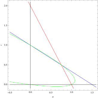
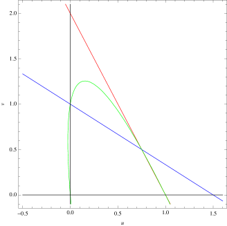
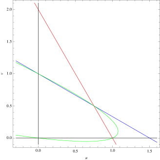
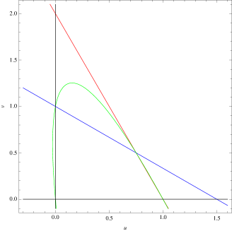
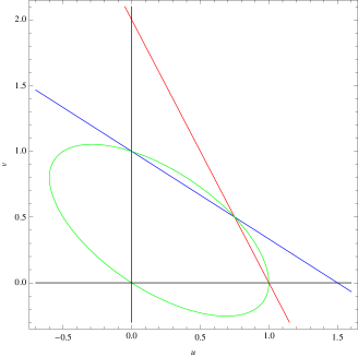
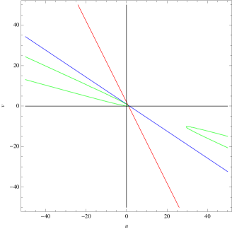
Figure 3.1: Red line: $\sigma_{1}-c_{11}\,u-c_{12}\,v=0$; blue line: $\sigma_{2}-c_{21}\,u-c_{22}\,v=0$; green curve: $\alpha\,u\,(\sigma_{1}-c_{11}\,u-c_{12}\,v)+\beta\,v\,(\sigma_{2}-c_{21}\,u-c_{22}\,v)=0$. $\sigma_{1}=\sigma_{2}=c_{11}=c_{22}=1,c_{12}=\frac{1}{2},c_{21}=\frac{2}{3}$. 3.1 $\alpha=\frac{1}{2}$, $\beta=4$ (hyperbola). 3.1 $\alpha=2$, $\beta=\frac{3}{20}$ (hyperbola). 3.1 $\alpha=2$, $\beta=\frac{15}{2}+3\sqrt{6}\approx 14.8485$ (parabola). 3.1 $\alpha=2$, $\beta=\frac{15}{2}-3\sqrt{6}\approx 0.1515$ (parabola). 3.1 $\alpha=2$, $\beta=3$ (ellipse). 3.1 zooming out of (a).

∎

Proof of Theorem 2.1.

An easy observation shows that, it suffices to prove for any $\alpha,\beta>0$, we have

$$q_{\ast}\leq\alpha\,d_{1}\,u(x)+\beta\,d_{2}\,v(x)\leq q^{\ast},\quad x\in\mathbb{R},$$ (3.2)

where

$$q_{\ast}=\min\bigg{[}\alpha\,d_{1}\,\min\Big{[}\frac{\sigma_{1}}{c_{11}},\frac{\sigma_{2}}{c_{21}}\Big{]},\beta\,d_{2}\,\min\Big{[}\frac{\sigma_{2}}{c_{22}},\frac{\sigma_{1}}{c_{12}}\Big{]}\bigg{]}\min\Big{[}\frac{d_{1}}{d_{2}},\frac{d_{2}}{d_{1}}\Big{]}$$ (3.3)

and

$$q^{\ast}=\max\bigg{[}\alpha\,d_{1}\,\max\Big{[}\frac{\sigma_{1}}{c_{11}},\frac{\sigma_{2}}{c_{21}}\Big{]},\beta\,d_{2}\,\max\Big{[}\frac{\sigma_{2}}{c_{22}},\frac{\sigma_{1}}{c_{12}}\Big{]}\bigg{]}\max\Big{[}\frac{d_{1}}{d_{2}},\frac{d_{2}}{d_{1}}\Big{]}.$$ (3.4)

First of all, we prove $(I)$ for the case of strong competition $\mathbf{[S]}$: $\frac{\sigma_{1}}{c_{11}}>\frac{\sigma_{2}}{c_{21}}$ and $\frac{\sigma_{2}}{c_{22}}>\frac{\sigma_{1}}{c_{12}}$. Clearly, (3.3) in this case gives

$$q(x)\geq\min\bigg{[}\alpha\,d_{1}\,\frac{\sigma_{2}}{c_{21}},\beta\,d_{2}\,\frac{\sigma_{1}}{c_{12}}\bigg{]}\min\Big{[}\frac{d_{1}}{d_{2}},\frac{d_{2}}{d_{1}}\Big{]},\quad x\in\mathbb{R}.$$ (3.5)

The proof of the above inequality is divided into the following four cases:

• If $d_{2}\geq d_{1}$,

  • when $\beta\,\sigma_{1}\,c_{21}\,d_{2}\geq\alpha\,\sigma_{2}\,c_{12}\,d_{1}$ and $(\lambda_{1},\lambda_{2},\eta)=\big{(}\frac{\alpha\,\sigma_{2}\,d_{1}^{2}}{c_{21}\,d_{2}},\frac{\alpha\,\sigma_{2}\,d_{1}}{c_{21}},\frac{\alpha\,\sigma_{2}\,d_{1}}{c_{21}\,d_{2}}\big{)}$, $q(x)\geq\lambda_{1}$, $x\in\mathbb{R}$;

  • when $\beta\,\sigma_{1}\,c_{21}\,d_{2}<\alpha\,\sigma_{2}\,c_{12}\,d_{1}$ and $(\lambda_{1},\lambda_{2},\eta)=\big{(}\frac{\beta\,\sigma_{1}\,d_{1}}{c_{12}},\frac{\beta\,\sigma_{1}\,d_{2}}{c_{12}},\frac{\beta\,\sigma_{1}}{c_{12}}\big{)}$, $q(x)\geq\lambda_{1}$, $x\in\mathbb{R}$.

• If $d_{2}<d_{1}$,

  • when $\beta\,\sigma_{1}\,c_{21}\,d_{2}\geq\alpha\,\sigma_{2}\,c_{12}\,d_{1}$ and $(\lambda_{1},\lambda_{2},\eta)=\big{(}\frac{\alpha\,\sigma_{2}\,d_{2}}{c_{21}},\frac{\alpha\,\sigma_{2}\,d_{1}}{c_{21}},\frac{\alpha\,\sigma_{2}}{c_{21}}\big{)}$, $q(x)\geq\lambda_{1}$, $x\in\mathbb{R}$;

  • when $\beta\,\sigma_{1}\,c_{21}\,d_{2}<\alpha\,\sigma_{2}\,c_{12}\,d_{1}$ and $(\lambda_{1},\lambda_{2},\eta)=\big{(}\frac{\beta\,\sigma_{1}\,d_{2}^{2}}{c_{12}\,d_{1}},\frac{\beta\,\sigma_{1}\,d_{2}}{c_{12}},\frac{\beta\,\sigma_{1}\,d_{2}}{c_{12}\,d_{1}}\big{)}$, $q(x)\geq\lambda_{1}$, $x\in\mathbb{R}$.

We first observe that the four cases can be reduced to the following two cases:

• for $\beta\,\sigma_{1}\,c_{21}\,d_{2}\geq\alpha\,\sigma_{2}\,c_{12}\,d_{1}$, $q(x)\geq\frac{\alpha\,\sigma_{2}\,d_{1}}{c_{21}}\min\big{[}\frac{d_{1}}{d_{2}},\frac{d_{2}}{d_{1}}\big{]}$, $x\in\mathbb{R}$;

• for $\beta\,\sigma_{1}\,c_{21}\,d_{2}<\alpha\,\sigma_{2}\,c_{12}\,d_{1}$, $q(x)\geq\frac{\beta\,\sigma_{1}\,d_{2}}{c_{12}}\min\big{[}\frac{d_{1}}{d_{2}},\frac{d_{2}}{d_{1}}\big{]}$, $x\in\mathbb{R}$.

Combining the two cases above leads to

$$q(x)\geq\min\bigg{[}\alpha\,d_{1}\,\frac{\sigma_{2}}{c_{21}},\beta\,d_{2}\,\frac{\sigma_{1}}{c_{12}}\bigg{]}\min\Big{[}\frac{d_{1}}{d_{2}},\frac{d_{2}}{d_{1}}\Big{]},\quad x\in\mathbb{R},$$ (3.6)

which is the desired result. The two inequalities in (2.4) give

$$q^{\prime\prime}(x)+\theta\,p^{\prime}(x)+F(u(x),v(x))\leq 0,\quad x\in\mathbb{R}.$$ (3.7)

For $d_{2}>d_{1}$, we prove $(i)$ by contradiction. Suppose that, contrary to our claim, there exists $z\in\mathbb{R}$ such that $q(z)<\lambda_{1}$ and $\min_{x\in\mathbb{R}}q(x)=q(z)$. Since $u,v\in C^{2}(\mathbb{R})$, we denote respectively by $z_{2}$ and $z_{1}$ the first point intersecting the line $\alpha\,d_{1}\,u+\beta\,d_{2}\,v=\lambda_{2}$ in the $uv$-plane, when the solution $(u(x),v(x))$ in the $uv$-plane travels from $z$ towards $\infty$ and $-\infty$ (as shown in Figure 3.3.2). For the case where $\theta\leq 0$, we integrate (3.7) with respect to $x$ from $z_{1}$ to $z$ and obtain

$$q^{\prime}(z)-q^{\prime}(z_{1})+\theta\,(p(z)-p(z_{1}))+\int_{z_{1}}^{z}F(u(x),v(x))\,dx\leq 0.$$ (3.8)

On the other hand we conclude:

• since $\min_{x\in\mathbb{R}}q(x)=q(z)$, it is easy to see $q^{\prime}(z)=\alpha\,d_{1}\,u^{\prime}(z)+\beta\,d_{2}\,v^{\prime}(z)=0$;

• $q(z_{1})=\lambda_{2}$ follows from the fact that $z_{1}$ is on the line $\alpha\,d_{1}\,u+\beta\,d_{2}\,v=\lambda_{2}$. On the other hand, when $z_{1}$ moves a little towards $\infty$, $q(z_{1}+)$ is below the line $\alpha\,d_{1}\,u+\beta\,d_{2}\,v=\lambda_{2}$. This leads to $q(z_{1}+\delta)\leq\lambda_{2}$ for any $\delta>0$, and hence $q^{\prime}(z_{1})\leq 0$;

• $p(z)<\eta$ since $z$ is below the line $\alpha\,u+\beta\,v=\eta$; $p(z_{1})>\eta$ since $z$ is above the line $\alpha\,u+\beta\,v=\eta$;

• it is readily seen that the quadratic curve $F(u,v)=0$ passes through the points $(0,0)$, $\big{(}\frac{\sigma_{1}}{c_{11}},0\big{)}$, $\big{(}0,\frac{\sigma_{2}}{c_{22}}\big{)}$, and $(u^{\ast},v^{\ast})$ in the $uv$-plane. Applying Lemma 3.1, it follows that $F(u,v)=0$ is a hyperbola and $\int_{z_{1}}^{z}F(u(x),v(x))\,dx>0$ since $F(u,v)<0$ as $u,v>0$ are sufficiently large.

Summarizing the above arguments, we obtain

$$q^{\prime}(z)-q^{\prime}(z_{1})+\theta\,(p(z)-p(z_{1}))+\int_{z_{1}}^{z}F(u(x),v(x))\,dx>0,$$ (3.9)

which contradicts (3.8). Therefore when $\theta\leq 0$, $q(x)\geq\lambda_{1}$ for $x\in\mathbb{R}$. For the case where $\theta\geq 0$, integrating (3.7) with respect to $x$ from $z$ to $z_{2}$ yields

$$q^{\prime}(z_{2})-q^{\prime}(z)+\theta\,(p(z_{2})-p(z))+\int_{z}^{z_{2}}F(u(x),v(x))\,dx\leq 0.$$ (3.10)

In a similar manner, it can be shown that $q^{\prime}(z_{2})>0$, $q^{\prime}(z)=0$, $p(z_{2})>\eta$, $p(z)<\eta$, and $\int_{z}^{z_{2}}F(u(x),v(x))\,dx>0$. These together contradict (3.10). Consequently, $(i)$ is proved for $d_{2}>d_{1}$. For $d_{1}=d_{2}$, we have $q(x)=p(x)$ and (3.7) becomes

$$p^{\prime\prime}(x)+\theta\,p^{\prime}(x)+F(u(x),v(x))\leq 0,\quad x\in\mathbb{R}.$$ (3.11)

Moreover, when $d_{1}=d_{2}$ we take $\frac{\lambda_{1}}{d_{1}}=\frac{\lambda_{2}}{d_{1}}=\eta=\frac{\alpha\,\sigma_{2}}{c_{21}}$, i.e. the three lines $\alpha\,d_{1}\,u+\beta\,d_{2}\,v=\lambda_{1}$, $\alpha\,d_{1}\,u+\beta\,d_{2}\,v=\lambda_{2}$, and $\alpha\,u+\beta\,v=\eta$ coincide. Analogously to the case of $d_{2}>d_{1}$, we assume that there exists $\hat{z}\in\mathbb{R}$ such that $p(\hat{z})<\lambda_{1}$ and $\min_{x\in\mathbb{R}}p(x)=p(\hat{z})$. Due to $\min_{x\in\mathbb{R}}p(x)=p(\hat{z})$, we have $p^{\prime}(\hat{z})=0$ and $p^{\prime\prime}(\hat{z})\geq 0$. By means of Lemma 3.1, $F(u(\hat{z}),v(\hat{z}))>0$. These together give $p^{\prime\prime}(\hat{z})+\theta\,p^{\prime}(\hat{z})+F(u(\hat{z}),v(\hat{z}))>0$, which contradicts (3.11). Thus, $p(x)\geq\lambda_{1}$ for $x\in\mathbb{R}$ when $d_{1}=d_{2}$. As a result, the proof of $(i)$ is completed.

Clearly, we see from Figures 3.3.2, 3.3.2, and 3.3.2 that the proofs of cases $(ii)$, $(iii)$, and $(iv)$ follow in a similar manner. This completes the proof of the case of strong competition $\mathbf{[S]}$: $\frac{\sigma_{1}}{c_{11}}>\frac{\sigma_{2}}{c_{21}}$ and $\frac{\sigma_{2}}{c_{22}}>\frac{\sigma_{1}}{c_{12}}$.

       

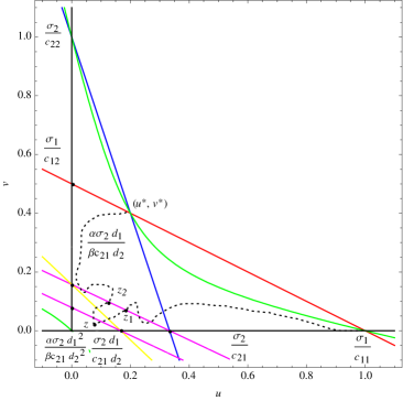
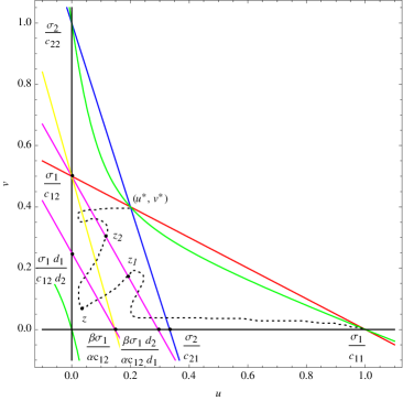
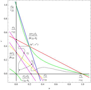
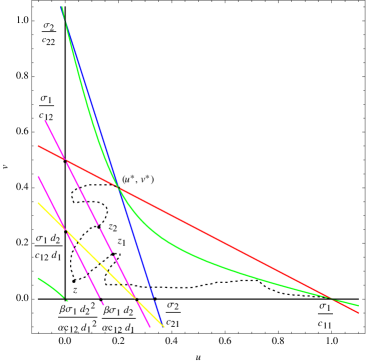
Figure 3.2: Red line: $\sigma_{1}-c_{11}\,u-c_{12}\,v=0$; blue line: $\sigma_{2}-c_{21}\,u-c_{22}\,v=0$; green curve: $\alpha\,u\,(\sigma_{1}-c_{11}\,u-c_{12}\,v)+\beta\,v\,(\sigma_{2}-c_{21}\,u-c_{22}\,v)=0$; magenta line (above): $\alpha\,d_{1}\,u+\beta\,d_{2}\,v=\lambda_{2}$; magenta line (below): $\alpha\,d_{1}\,u+\beta\,d_{2}\,v=\lambda_{1}$; yellow line: $\alpha\,u+\beta\,v=\eta$; dashed curve: $(u(x),v(x))$. $d_{1}=\sigma_{1}=\sigma_{2}=c_{11}=c_{22}=1$. 3.2 $c_{12}=2$, $c_{21}=3$, $\alpha=17$, $\beta=18$, and $d_{2}=2$ give $\lambda_{1}=\frac{17}{6}$, $\lambda_{2}=\frac{17}{3}$, and $\eta=\frac{17}{6}$. 3.2 $c_{12}=2$, $c_{21}=3$, $\alpha=17$, $\beta=5$, and $d_{2}=2$ give $\lambda_{1}=\frac{5}{2}$, $\lambda_{2}=5$, and $\eta=\frac{5}{2}$. 3.2 $c_{12}=2$, $c_{21}=3$, $\alpha=17$, $\beta=18$, and $d_{2}=\frac{2}{3}$ give $\lambda_{1}=\frac{34}{9}$, $\lambda_{2}=\frac{17}{3}$, and $\eta=\frac{17}{3}$. 3.2 $c_{12}=2$, $c_{21}=3$, $\alpha=17$, $\beta=18$, and $d_{2}=\frac{1}{2}$ give $\lambda_{1}=\frac{9}{4}$, $\lambda_{2}=\frac{9}{2}$, and $\eta=\frac{9}{2}$.

To give the proof for the case of weak competition $\mathbf{[W]}$: $\frac{\sigma_{1}}{c_{11}}<\frac{\sigma_{2}}{c_{21}}$ and $\frac{\sigma_{2}}{c_{22}}<\frac{\sigma_{1}}{c_{12}}$, which leads to

$$q(x)\geq\min\bigg{[}\alpha\,d_{1}\,\frac{\sigma_{1}}{c_{11}},\beta\,d_{2}\,\frac{\sigma_{2}}{c_{22}}\bigg{]}\min\Big{[}\frac{d_{1}}{d_{2}},\frac{d_{2}}{d_{1}}\Big{]},\quad x\in\mathbb{R}$$ (3.12)

by (3.3), we first see from Lemma 3.1 that $F(u,v)=0$ in this case is a hyperbola (see for example Figure 3.3.1, Figure 3.3.1, and Figure 3.3.1) as in the case of strong competition $\mathbf{[S]}$, a parabola (see for example Figure 3.3.1 and Figure 3.3.1), or an ellipse (see for example Figure 3.3.1) depending on the parameters in $F(u,v)=0$. However, since we are only concerned with the curve $F(u,v)=0$ in the first quadrant of the $uv$-plane, it is readily seen from Figure 3.1 that for each of the three generic types of quadratic curves, we can construct an N-barrier for which the arguments used in proving the case of strong competition $\mathbf{[S]}$ remain valid. Moreover, in addition to the diffusion rates $d_{1}$, $d_{2}$ and the coefficients $\alpha$, $\beta$, the lower bound of $q(x)$ given by (3.5) under $\mathbf{[S]}$ is only involved with the minimal $u$-intercept of the lines $\sigma_{1}-c_{11}\,u-c_{12}\,v=0$ and $\sigma_{2}-c_{21}\,u-c_{22}\,v=0$, i.e. $u=\frac{\sigma_{2}}{c_{21}}$, and the minimal $v$-intercept of the lines $\sigma_{1}-c_{11}\,u-c_{12}\,v=0$ and $\sigma_{2}-c_{21}\,u-c_{22}\,v=0$, i.e. $v=\frac{\sigma_{1}}{c_{12}}$. Accordingly, for the case of weak competition $\mathbf{[W]}$, we conclude that (3.12) holds since the minimal $u$-intercept of the lines $\sigma_{1}-c_{11}\,u-c_{12}\,v=0$ and $\sigma_{2}-c_{21}\,u-c_{22}\,v=0$ is $u=\frac{\sigma_{1}}{c_{11}}$, and the minimal $v$-intercept of the lines $\sigma_{1}-c_{11}\,u-c_{12}\,v=0$ and $\sigma_{2}-c_{21}\,u-c_{22}\,v=0$ is $v=\frac{\sigma_{2}}{c_{22}}$, respectively. For the case of strong competition $\mathbf{[S]}$, (3.5) is proved, whereas for the case of weak competition $\mathbf{[W]}$, we obtain (3.12). Combining the two inequalities (3.5) and (3.12) yields the lower bound of $q(x)$ given by (3.3). This completes the proof of $(I)$.

As in the proof of $(I)$, there are also four cases for the proof of $(II)$ when the condition of strong competition $\mathbf{[S]}$ holds:

• If $d_{2}\geq d_{1}$,

  • when $\beta\,\sigma_{2}\,c_{11}\,d_{2}\geq\alpha\,\sigma_{1}\,c_{22}\,d_{1}$ and $(\lambda_{1},\lambda_{2},\eta)=\big{(}\frac{\beta\,\sigma_{2}\,d_{2}^{2}}{c_{22}\,d_{1}},\frac{\beta\,\sigma_{2}\,d_{2}}{c_{22}},\frac{\sigma_{2}\,d_{2}}{c_{22}\,d_{1}}\big{)}$, $q(x)\leq\lambda_{1}$, $x\in\mathbb{R}$;

  • when $\beta\,\sigma_{2}\,c_{11}\,d_{2}<\alpha\,\sigma_{1}\,c_{22}\,d_{1}$ and $(\lambda_{1},\lambda_{2},\eta)=\big{(}\frac{\alpha\,\sigma_{1}\,d_{2}}{c_{11}},\frac{\alpha\,\sigma_{1}\,d_{1}}{c_{11}},\frac{\alpha\,\sigma_{1}}{c_{11}}\big{)}$, $q(x)\leq\lambda_{1}$, $x\in\mathbb{R}$.

• If $d_{2}<d_{1}$,

  • when $\beta\,\sigma_{2}\,c_{11}\,d_{2}\geq\alpha\,\sigma_{1}\,c_{22}\,d_{1}$ and $(\lambda_{1},\lambda_{2},\eta)=\big{(}\frac{\beta\,\sigma_{2}\,d_{1}}{c_{22}},\frac{\beta\,\sigma_{2}\,d_{2}}{c_{22}},\frac{\beta\,\sigma_{2}}{c_{22}}\big{)}$, $q(x)\leq\lambda_{1}$, $x\in\mathbb{R}$;

  • when $\beta\,\sigma_{2}\,c_{11}\,d_{2}<\alpha\,\sigma_{1}\,c_{22}\,d_{1}$ and $(\lambda_{1},\lambda_{2},\eta)=\big{(}\frac{\alpha\,\sigma_{1}\,d_{1}^{2}}{c_{11}\,d_{2}},\frac{\alpha\,\sigma_{1}\,d_{1}}{c_{11}},\frac{\alpha\,\sigma_{1}\,d_{1}}{c_{11}\,d_{2}}\big{)}$, $q(x)\leq\lambda_{1}$, $x\in\mathbb{R}$.

Combining the four cases above, it immediately follows that

• for $\beta\,\sigma_{2}\,c_{11}\,d_{2}\geq\alpha\,\sigma_{1}\,c_{22}\,d_{1}$, $q(x)\leq\frac{\beta\,\sigma_{2}\,d_{2}}{c_{22}}\max\big{[}\frac{d_{1}}{d_{2}},\frac{d_{2}}{d_{1}}\big{]}$ for $x\in\mathbb{R}$;

• for $\beta\,\sigma_{2}\,c_{11}\,d_{2}<\alpha\,\sigma_{1}\,c_{22}\,d_{1}$, $q(x)\leq\frac{\alpha\,\sigma_{1}\,d_{1}}{c_{11}}\max\big{[}\frac{d_{1}}{d_{2}},\frac{d_{2}}{d_{1}}\big{]}$ for $x\in\mathbb{R}$,

and hence we have

$$q(x)\leq\max\bigg{[}\alpha\,d_{1}\,\frac{\sigma_{1}}{c_{11}},\beta\,d_{2}\,\frac{\sigma_{2}}{c_{22}}\bigg{]}\max\Big{[}\frac{d_{1}}{d_{2}},\frac{d_{2}}{d_{1}}\Big{]},\quad x\in\mathbb{R}.$$ (3.13)

Indeed, (3.13) holds, as is readily seen by employing similar arguments as above together with the N-barriers constructed in Figures 3.3.3, 3.3.3, 3.3.3, and 3.3.3. On the other hand, under the condition of weak competition $\mathbf{[W]}$, (3.4) leads to

$$q(x)\leq\max\bigg{[}\alpha\,d_{1}\,\frac{\sigma_{2}}{c_{21}},\beta\,d_{2}\,\frac{\sigma_{1}}{c_{12}}\bigg{]}\max\Big{[}\frac{d_{1}}{d_{2}},\frac{d_{2}}{d_{1}}\Big{]},\quad x\in\mathbb{R},$$ (3.14)

which can be shown as in the proof of (3.12) by interchanging the roles of $\frac{\sigma_{1}}{c_{11}}$ ($\frac{\sigma_{2}}{c_{22}}$, respectively) and $\frac{\sigma_{2}}{c_{21}}$ ($\frac{\sigma_{1}}{c_{12}}$, respectively) in (3.13). Therefore $(II)$ of Theorem 2.1 follows from (3.13) and (3.14). The proof of Theorem 2.1 is completed.

       

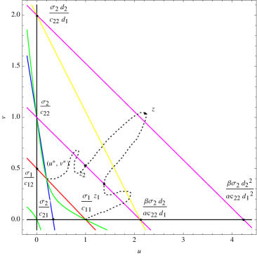
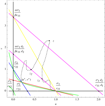
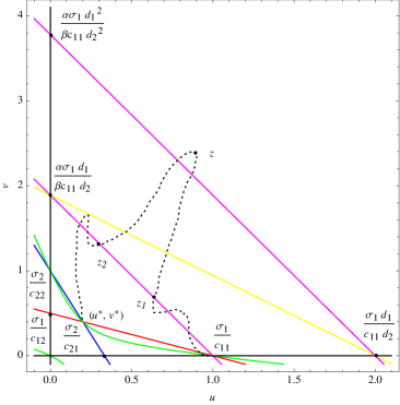
Figure 3.3: Red line: $\sigma_{1}-c_{11}\,u-c_{12}\,v=0$; blue line: $\sigma_{2}-c_{21}\,u-c_{22}\,v=0$; green curve: $\alpha\,u\,(\sigma_{1}-c_{11}\,u-c_{12}\,v)+\beta\,v\,(\sigma_{2}-c_{21}\,u-c_{22}\,v)=0$; magenta line (below): $\alpha\,d_{1}\,u+\beta\,d_{2}\,v=\lambda_{2}$; magenta line (above): $\alpha\,d_{1}\,u+\beta\,d_{2}\,v=\lambda_{1}$; yellow line: $\alpha\,u+\beta\,v=\eta$; dashed curve: $(u(x),v(x))$. $d_{1}=\sigma_{1}=\sigma_{2}=c_{11}=c_{22}=1$. 3.3 $c_{12}=2$, $c_{21}=3$, $\alpha=17$, $\beta=18$, and $d_{2}=2$ give $\lambda_{1}=72$, $\lambda_{2}=36$, and $\eta=36$. 3.3 $c_{12}=2$, $c_{21}=3$, $\alpha=17$, $\beta=5$, and $d_{2}=2$ give $\lambda_{1}=34$, $\lambda_{2}=17$, and $\eta=17$. 3.3 $c_{12}=2$, $c_{21}=3$, $\alpha=17$, $\beta=33$, and $d_{2}=\frac{2}{3}$ give $\lambda_{1}=33$, $\lambda_{2}=22$, and $\eta=33$. 3.3 $c_{12}=2$, $c_{21}=3$, $\alpha=17$, $\beta=18$, and $d_{2}=\frac{1}{2}$ give $\lambda_{1}=34$, $\lambda_{2}=17$, and $\eta=34$.

∎

4 New exact $(1,0,0)$-$(u^{\ast},v^{\ast},0)$ waves

In this section, we always assume $\sigma_{1}=c_{11}$, unless otherwise stated. Looking for traveling wave solutions $(u(x),v(x),w(x))$ with the profiles of $u(x)$ being decreasing in $x$, $v(x)$ being increasing in $x$, and $w(x)$ being a pulse (i.e., $w(\pm\infty)=0$ and $w(x)>0$ for $x\in\mathbb{R}$) of (2.16) leads to the following ansätz ([6, 7, 8, 19]) for solving (2.16)

$$\begin{cases}\vspace{3mm}u(x)=\frac{\displaystyle 1}{\displaystyle 2}(u^{\ast}+1)+\frac{\displaystyle 1}{\displaystyle 2}(u^{\ast}-1)\,T(x),\\ \vspace{3mm}v(x)=k_{1}\,(1+T(x))^{2},\\ w(x)=k_{2}\,(1-T^{2}(x)),\end{cases}$$ (4.1)

where $T(x)=\tanh(x)$, $k_{1}=\frac{\displaystyle v^{\ast}}{\displaystyle 4}$ and $k_{2}$ is a positive constant to be determined. It is readily verified that the ansätz (4.1) satisfies the boundary conditions at $x=\pm\infty$ in (2.16). Since $u(x)$, $v(x)$ and $w(x)$ in (4.1) are expressed in terms of polynomials in $\tanh(x)$ and $\frac{d}{dx}\tanh(x)=1-\tanh^{2}(x)$, inserting (4.1) into the three equations in (2.16) gives

$$d_{1}\,u_{xx}+\theta\,u_{x}+u\,(\sigma_{1}-c_{11}\,u-c_{12}\,v-c_{13}\,w)=\Big{[}\zeta_{10}+\zeta_{11}\,T(x)+\zeta_{12}\,{T^{2}(x)}+\zeta_{13}\,{T^{3}(x)}\,\Big{]},$$ (4.2a)

$$d_{2}\,v_{xx}+\theta\,v_{x}+v\,(\sigma_{2}-c_{21}\,u-c_{22}\,v-c_{23}\,w)=v\,\Big{[}\zeta_{20}+\zeta_{21}\,T(x)+\zeta_{22}\,{T^{2}(x)}\,\Big{]},$$ (4.2b)

$$d_{3}\,w_{xx}+\theta\,w_{x}+w\,(\sigma_{3}-c_{31}\,u-c_{32}\,v-c_{33}\,w)=w\,\Big{[}\zeta_{30}+\zeta_{31}\,T(x)+\zeta_{32}\,{T^{2}(x)}\,\Big{]}.$$ (4.2c)

Equating the coefficients of powers of $T(x)$ to zero yields a system of ten algebraic equations:

$$\begin{cases}\vspace{2mm}\zeta_{1i}=0,\;i=0,1,2,3,\\ \vspace{2mm}\zeta_{2i}=0,\;i=0,1,2,\\ \zeta_{3i}=0,\;i=0,1,2.\\ \end{cases}$$ (4.3)

It turns out that (4.2) can be solved to give

$$c_{11}=\sigma_{1},$$ (4.4a)

$$c_{12}=\frac{d_{1}\sigma_{1}}{k_{1}\left(2d_{1}+\theta\right)},$$ (4.4b)

$$c_{13}=\frac{-2d_{1}\theta+d_{1}\sigma_{1}-4d_{1}^{2}}{k_{2}\left(2d_{1}+\theta\right)},$$ (4.4c)

$$c_{21}=16d_{2}+4\theta+\sigma_{2},$$ (4.4d)

$$c_{22}=\frac{2d_{1}\theta-4d_{2}\theta+d_{1}\sigma_{2}+8d_{1}d_{2}-\theta^{2}}{k_{1}\left(2d_{1}+\theta\right)},$$ (4.4e)

$$c_{23}=\frac{2d_{1}\theta-10d_{2}\theta+d_{1}\sigma_{2}-4d_{1}d_{2}-\theta^{2}}{k_{2}\left(2d_{1}+\theta\right)},$$ (4.4f)

$$c_{31}=4d_{3}+2\theta+\sigma_{3},$$ (4.4g)

$$c_{32}=\frac{d_{1}\sigma_{3}+4d_{1}d_{3}-\theta^{2}}{k_{1}\left(2d_{1}+\theta\right)},$$ (4.4h)

$$c_{33}=\frac{-6d_{3}\theta+d_{1}\sigma_{3}-8d_{1}d_{3}-\theta^{2}}{k_{2}\left(2d_{1}+\theta\right)}.$$ (4.4i)

The result obtained is summarized in the following theorem.

Theorem 4.1 (Exact $(1,0,0)$-$(u^{\ast},v^{\ast},0)$ waves).

The boundary value problem (2.16) with $\sigma_{1}=c_{11}$ admits an exact solution of the form (4.1) provided that (4.4) holds.

Theorem 4.1 asserts that under certain conditions imposed on the parameters, i.e. under (4.4), we can find exact $(1,0,0)$-$(u^{\ast},v^{\ast},0)$ waves of (2.16) and the exact waves are polynomials in $\tanh(x)$. To illustrate Theorem 4.1, let us choose $k_{1}=k_{2}=d_{1}=d_{2}=d_{3}=1$, $\theta=3$, and $\sigma_{1}=\sigma_{2}=\sigma_{3}=41$ in (4.4). This gives $c_{11}=41,c_{12}=\frac{41}{5},c_{13}=\frac{31}{5},c_{21}=69,c_{22}=\frac{34}{5},c_{23}=\frac{4}{5},c_{31}=51,c_{32}=\frac{36}{5},c_{33}=\frac{6}{5}$ and $(u^{\ast},v^{\ast})=(\frac{1}{5},4)$. The resulting exact $(1,0,0)$-$(u^{\ast},v^{\ast},0)$ wave is given by

$$\begin{cases}\vspace{3mm}u(x)=\frac{\displaystyle 3}{\displaystyle 5}-\frac{\displaystyle 2}{\displaystyle 5}\,\tanh(x),\\ \vspace{3mm}v(x)=(1+\tanh(x))^{2},\\ w(x)=1-\tanh^{2}(x).\end{cases}$$ (4.5)

The profiles of $u(x)$, $v(x)$, and $w(x)$ are shown in Figure 4.1.

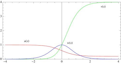
Figure 4.1: Profiles of the solution $(u(x),v(x),w(x))$.

We conclude this section with the remark that the ansätz (4.1) for solutions of (2.16) is inspired by the one proposed in [19], where the ansätz (4.1) for solutions is

$$\begin{cases}\vspace{3mm}u(x)=\frac{\displaystyle 1}{\displaystyle 2}(u^{\ast}+1)+\frac{\displaystyle 1}{\displaystyle 2}(u^{\ast}-1)\,T(x),\\ v(x)=k_{1}\,(1+T(x))^{2},\\ \end{cases}$$ (4.6)

when $w$ is absent in (2.16).

5 Applications of the N-barrier maximum principle

5.1 Application to the existence of three species traveling waves: proof of Theorem 2.2

To prove Theorem 2.2, we first observe that the third equation in (2.17) can be regarded as a non-autonomous Fisher equation when $u=u(x)$ and $v=v(x)$ are given, say $u=\tilde{u}(x)$ and $v=\tilde{v}(x)$. Then the non-autonomous Fisher equation ([4], [32], [37]) is

$$d_{3}\,w_{xx}+\theta\,w_{x}+w\,(\sigma_{3}-c_{31}\,\tilde{u}-c_{32}\,\tilde{v}-c_{33}\,w)=0,\quad x\in\mathbb{R}.$$ (5.1)

In order to find a solution of (5.1), an approach based on the supersolution-subsolution method is employed. To this end, we introduce supersolutions and subsolutions. $\bar{w}=\bar{w}(x)$ is said to be a supersolution of (5.1) if it satisfies the differential inequality

$$d_{3}\,\bar{w}_{xx}+\theta\,\bar{w}_{z}+\bar{w}\,(\sigma_{3}-c_{31}\,\tilde{u}-c_{32}\,\tilde{v}-c_{33}\,\bar{w})\leq 0,\quad x\in\mathbb{R}.$$ (5.2)

Similarly, a subsolution $\underaccent{\bar}{w}=\underaccent{\bar}{w}(x)$ is defined by reversing the inequality in (5.2). The following lemma is helpful in constructing non-trivial solutions of (5.1).

Lemma 5.1 ([4]).

Suppose that $w(x)$ is a bounded solution of

$$d_{3}\,w_{xx}+\theta\,w_{x}+w\,\varphi(w,x)=0,\quad x\in\mathbb{R},$$ (5.3)

where $\varphi(0,x)\rightarrow-{\varphi_{0}}^{\pm}$ as $x\rightarrow\pm\infty$ for some constants ${\varphi_{0}}^{+},{\varphi_{0}}^{-}>0$. Then $w(x)\rightarrow 0$ as $x\rightarrow\pm\infty$.

To construct a pair of subsolution and supersolution of (5.1), we employ the tanh method.

Proof of Theorem 2.2.

Due to $\mathbf{[H4]}$, we clearly have $\underaccent{\bar}{w}(x)\leq\bar{w}(x)$ for $x\in\mathbb{R}$. First of all, we show that $\underaccent{\bar}{w}(x)$ and $\bar{w}(x)$ are a subsolution and a supersolution of (5.1) respectively. Indeed, a straightforward computation gives us

$$d_{3}\,\underaccent{\bar}{w}_{xx}+\theta\,\underaccent{\bar}{w}_{z}+\underaccent{\bar}{w}\,(\,\sigma_{3}-c_{31}\,\tilde{u}-c_{32}\,\tilde{v}-c_{33}\,\underaccent{\bar}{w})$$

$$=\underaccent{\bar}{w}\,\big{[}-c_{33}\,\underaccent{\bar}{K}-2\,d_{3}-\bar{q}+\sigma_{3}-2\,\theta\,\tanh(x)+(c_{33}\,\underaccent{\bar}{K}+6\,d_{3})\,\tanh^{2}(x)\big{]}\geq 0,$$

$$d_{3}\,\bar{w}_{xx}+\theta\,\bar{w}_{z}+\bar{w}\,(\,\sigma_{3}-c_{31}\,\tilde{u}-c_{32}\,\tilde{v}-c_{33}\,\bar{w})$$

$$=\bar{w}\,\big{(}-c_{33}\,\bar{K}-\underaccent{\bar}{q}+\sigma_{3}\big{)}\leq 0$$ (5.4)

under hypotheses $\mathbf{[H2]}$ and $\mathbf{[H3]}$. By means of Theorem 2.1, we have used in the last two inequalities an estimate of $c_{31}\,\tilde{u}(x)+c_{32}\,\tilde{v}(x)$, i.e.

$$\underaccent{\bar}{q}\leq c_{31}\,\tilde{u}(x)+c_{32}\,\tilde{v}(x)\leq\bar{q},\quad x\in\mathbb{R}.$$ (5.5)

The existence of a solution $w=w(x)$ for (5.1) lying between the subsolution $\underaccent{\bar}{w}(x)$ and the supersolution $\bar{w}(x)$ constructed above follows from Theorem 2.8 in [26]. In view of $\mathbf{[H1]}$, we finally employ Lemma 5.1 to conclude that the solution $w(x)$ of (5.1) has the asymptotic behavior $\lim_{|x|\rightarrow\infty}w(x)=0$. This completes the proof. ∎

5.2 Application to the nonexistence of three species traveling waves: proof of Theorem 2.3

Proof of Theorem 2.3.

We prove Theorem 2.3 by contradiction. Suppose that, to the contrary, there exist $u(x),v(x),w(x)>0$, $x\in\mathbb{R}$ satisfying (2.16). Since $w(x)>0$ for $x\in\mathbb{R}$ and $w(\pm\infty)=0$, there exists $x_{0}\in\mathbb{R}$ such that $\max_{x\in\mathbb{R}}w(x)=w(x_{0})>0$, $w^{\prime\prime}(x_{0})<0$, and $w^{\prime}(x_{0})=0$. Due to $d_{3}\,w_{xx}+\theta\,w_{x}+w(\sigma_{3}-c_{31}\,u-c_{32}\,v-c_{33}\,w)=0$, we obtain

$$\sigma_{3}-c_{31}\,u(x_{0})-c_{32}\,v(x_{0})-c_{33}\,w(x_{0})>0,$$ (5.6)

and hence

$$w(x)\leq w(x_{0})<\frac{1}{c_{33}}\big{(}\sigma_{3}-c_{31}\,u(x_{0})-c_{32}\,v(x_{0})\big{)}<\frac{\sigma_{3}}{c_{33}},\;x\in\mathbb{R}.$$ (5.7)

As a result, we have

$$\begin{cases}\vspace{3mm}d_{1}\,u_{xx}+\theta\,u_{x}+u(\sigma_{1}-c_{13}\,\sigma_{3}\,c_{33}^{-1}-c_{11}\,u-c_{12}\,v)\leq 0,\quad x\in\mathbb{R},\\ d_{2}\,v_{xx}\hskip 2.27621pt+\theta\,v_{x}+v(\sigma_{2}-c_{23}\,\sigma_{3}\,c_{33}^{-1}-c_{21}\,u-c_{22}\,v)\leq 0,\quad x\in\mathbb{R}.\end{cases}$$ (5.8)

Because of $\mathbf{[A1]}$ and $\mathbf{[A2]}$, we can apply $(I)$ of Theorem 2.1 to (5.8). Indeed, $\mathbf{[A1]}$ assures the positivity of $\sigma_{1}-c_{13}\,\sigma_{3}\,c_{33}^{-1}$ and $\sigma_{2}-c_{23}\,\sigma_{3}\,c_{33}^{-1}$, whereas the assumption of strong competition $\mathbf{[S]}$ or the assumption of weak competition $\mathbf{[W]}$ for the nonlinearity in (5.8) follows from $\mathbf{[A2]}$. Consequently, $(I)$ of Theorem 2.1 gives us a lower bound of $c_{31}\,u(x)+c_{32}\,v(x)$, i.e. for $x\in\mathbb{R}$,

$$c_{31}\,u(x)+c_{32}\,v(x)\geq c_{33}^{-1}\,\min\bigg{[}c_{31}\,d_{1}\min\Big{[}\frac{\displaystyle\Sigma_{1}}{\displaystyle c_{11}},\frac{\displaystyle\Sigma_{2}}{\displaystyle c_{21}}\Big{]},c_{32}\,d_{2}\min\Big{[}\frac{\displaystyle\Sigma_{2}}{\displaystyle c_{22}},\frac{\displaystyle\Sigma_{1}}{\displaystyle c_{12}}\Big{]}\bigg{]}\min\Big{[}\frac{\displaystyle d_{1}}{\displaystyle d_{2}},\frac{\displaystyle d_{2}}{\displaystyle d_{1}}\Big{]}.$$ (5.9)

The condition $\mathbf{[A3]}$ then yields

$$c_{31}\,u(x)+c_{32}\,v(x)\geq\sigma_{3},\;x\in\mathbb{R},$$ (5.10)

which contradicts (5.6). This completes the proof of the theorem.

∎

Acknowledgments. The author would like to express gratitude to Dr. Tom Mollee for his careful reading of the manuscript and valuable comments to improve the readability of the paper. The author is also grateful for inspiring discussions with and constructive suggestions from Prof. Chiun-Chuan Chen.

References

- [1] M. W. Adamson and A. Y. Morozov, Revising the role of species mobility in maintaining biodiversity in communities with cyclic competition, Bull. Math. Biol., 74 (2012), pp. 2004–2031.
- [2] R. A. Armstrong and R. McGehee, Competitive exclusion, Amer. Natur., 115 (1980), pp. 151–170.
- [3] A. J. Baczkowski, D. N. Joanes, and G. M. Shamia, Range of validity of and for a generalized diversity index due to Good, Math. Biosci., 148 (1998), pp. 115–128.
- [4] H. Berestycki, O. Diekmann, C. J. Nagelkerke, and P. A. Zegeling, Can a species keep pace with a shifting climate?, Bull. Math. Biol., 71 (2009), pp. 399–429.
- [5] R. S. Cantrell and J. R. Ward, Jr., On competition-mediated coexistence, SIAM J. Appl. Math., 57 (1997), pp. 1311–1327.
- [6] C.-C. Chen and L.-C. Hung, Nonexistence of traveling wave solutions, exact and semi-exact traveling wave solutions for diffusive lotka-volterra systems of three competing species, Communications on Pure and Applied Analysis, To appear.
- [7] C.-C. Chen, L.-C. Hung, M. Mimura, M. Tohma, and D. Ueyama, Semi-exact equilibrium solutions for three-species competition-diffusion systems, Hiroshima Math J., 43 (2013), pp. 176–206.
- [8] C.-C. Chen, L.-C. Hung, M. Mimura, and D. Ueyama, Exact travelling wave solutions of three-species competition-diffusion systems, Discrete Contin. Dyn. Syst. Ser. B, 17 (2012), pp. 2653–2669.
- [9] P. de Mottoni, Qualitative analysis for some quasilinear parabolic systems, Institute of Math., Polish Academy Sci., zam, 11 (1979), p. 190.
- [10] S.-I. Ei, R. Ikota, and M. Mimura, Segregating partition problem in competition-diffusion systems, Interfaces Free Bound., 1 (1999), pp. 57–80.
- [11] I. J. Good, The population frequencies of species and the estimation of population parameters, Biometrika, 40 (1953), pp. 237–264.
- [12] S. Grossberg, Decisions, patterns, and oscillations in nonlinear competitve systems with applications to Volterra-Lotka systems, J. Theoret. Biol., 73 (1978), pp. 101–130.
- [13] M. Gyllenberg and P. Yan, On a conjecture for three-dimensional competitive Lotka-Volterra systems with a heteroclinic cycle, Differ. Equ. Appl., 1 (2009), pp. 473–490.
- [14] T. G. Hallam, L. J. Svoboda, and T. C. Gard, Persistence and extinction in three species Lotka-Volterra competitive systems, Math. Biosci., 46 (1979), pp. 117–124.
- [15] M. W. Hirsch, Differential equations and convergence almost everywhere in strongly monotone semiflows, Contemp. Math, 17 (1983), pp. 267–285.
- [16] X. Hou and A. W. Leung, Traveling wave solutions for a competitive reaction-diffusion system and their asymptotics, Nonlinear Anal. Real World Appl., 9 (2008), pp. 2196–2213.
- [17] S.-B. Hsu and T.-H. Hsu, Competitive exclusion of microbial species for a single nutrient with internal storage, SIAM J. Appl. Math., 68 (2008), pp. 1600–1617.
- [18] S. B. Hsu, H. L. Smith, and P. Waltman, Competitive exclusion and coexistence for competitive systems on ordered Banach spaces, Trans. Amer. Math. Soc., 348 (1996), pp. 4083–4094.
- [19] L.-C. Hung, Exact traveling wave solutions for diffusive Lotka-Volterra systems of two competing species, Jpn. J. Ind. Appl. Math., 29 (2012), pp. 237–251.
- [20] S. R.-J. Jang, Competitive exclusion and coexistence in a Leslie-Gower competition model with Allee effects, Appl. Anal., 92 (2013), pp. 1527–1540.
- [21] J. I. Kanel, On the wave front solution of a competition-diffusion system in population dynamics, Nonlinear Anal., 65 (2006), pp. 301–320.
- [22] J. I. Kanel and L. Zhou, Existence of wave front solutions and estimates of wave speed for a competition-diffusion system, Nonlinear Anal., 27 (1996), pp. 579–587.
- [23] J. Kastendiek, Competitor-mediated coexistence: interactions among three species of benthic macroalgae, Journal of Experimental Marine Biology and Ecology, 62 (1982), pp. 201–210.
- [24] K. Kishimoto and H. F. Weinberger, The spatial homogeneity of stable equilibria of some reaction-diffusion systems on convex domains, J. Differential Equations, 58 (1985), pp. 15–21.
- [25] W. Ko, K. Ryu, and I. Ahn, Coexistence of three competing species with non-negative cross-diffusion rate, J. Dyn. Control Syst., 20 (2014), pp. 229–240.
- [26] P. Koch Medina and G. Schätti, Long-time behaviour for reaction-diffusion equations on , Nonlinear Anal., 25 (1995), pp. 831–870.
- [27] R. S. Maier, The integration of three-dimensional Lotka-Volterra systems, Proc. R. Soc. Lond. Ser. A Math. Phys. Eng. Sci., 469 (2013), pp. 20120693, 27.
- [28] R. McGehee and R. A. Armstrong, Some mathematical problems concerning the ecological principle of competitive exclusion, J. Differential Equations, 23 (1977), pp. 30–52.
- [29] M. Mimura and M. Tohma, Dynamic coexistence in a three-species competition–diffusion system, Ecological Complexity, 21 (2015), pp. 215–232.
- [30] S. Petrovskii, K. Kawasaki, F. Takasu, and N. Shigesada, Diffusive waves, dynamical stabilization and spatio-temporal chaos in a community of three competitive species, Japan J. Indust. Appl. Math., 18 (2001), pp. 459–481.
- [31] H. Ramezani and S. Holm, Sample based estimation of landscape metrics; accuracy of line intersect sampling for estimating edge density and Shannon’s diversity index, Environ. Ecol. Stat., 18 (2011), pp. 109–130.
- [32] L. Sanchez, A note on a nonautonomous O.D.E. related to the Fisher equation, J. Comput. Appl. Math., 113 (2000), pp. 201–209.
- [33] E. H. Simpson, Measurement of diversity., Nature, (1949).
- [34] H. L. Smith and P. Waltman, Competition for a single limiting resource in continuous culture: the variable-yield model, SIAM J. Appl. Math., 54 (1994), pp. 1113–1131.
- [35] P. van den Driessche and M. L. Zeeman, Three-dimensional competitive Lotka-Volterra systems with no periodic orbits, SIAM J. Appl. Math., 58 (1998), pp. 227–234.
- [36] A. I. Volpert, V. A. Volpert, and V. A. Volpert, Traveling wave solutions of parabolic systems, vol. 140 of Translations of Mathematical Monographs, American Mathematical Society, Providence, RI, 1994. Translated from the Russian manuscript by James F. Heyda.
- [37] V. A. Volpert and Y. M. Suhov, Stationary solutions of non-autonomous Kolmogorov-Petrovsky-Piskunov equations, Ergodic Theory Dynam. Systems, 19 (1999), pp. 809–835.
- [38] M. L. Zeeman, Hopf bifurcations in competitive three-dimensional Lotka-Volterra systems, Dynam. Stability Systems, 8 (1993), pp. 189–217.