Mid-Infrared Luminosity Function of Local Star-Forming Galaxies in the NEP-Wide Survey Field of AKARI

Abstract

We present mid-infrared (MIR) luminosity functions (LFs) of local ($z<0.3$) star-forming (SF) galaxies in the AKARI’s NEP-Wide Survey field. In order to derive more accurate luminosity function, we used spectroscopic sample only. Based on the NEP-Wide point source catalogue containing a large number of infrared (IR) sources distributed over the wide (5.4 deg²) field, we incorporated the spectroscopic redshift ($z$) data for $\sim$ 1790 selected targets obtained by optical follow-up surveys with MMT/Hectospec and WIYN/Hydra. The AKARI’s continuous 2 – 24$\mu$m wavelength coverage as well as photometric data from optical $u^{*}$ band to near-infrared $H-$band with the spectroscopic redshifts for our sample galaxies enable us to derive accurate spectral energy distributions (SEDs) in the mid-infrared. We carried out SED-fit analysis and employed $1/V_{max}$ method to derive the MIR (e.g., 8 $\mu$m, 12 $\mu$m, and 15 $\mu$m rest-frame) luminosity functions. We fit our 8 $\mu$m LFs to the double power-law with the power index of $\alpha=1.53$ and $\beta=2.85$ at the break luminosity $4.95\times 10^{9}L_{\odot}$. We made extensive comparisons with various MIR LFs from several literatures. Our results for local galaxies from the NEP region are generally consistent with other works for different fields over wide luminosity ranges. The comparisons with the results from the NEP-Deep data as well as other LFs imply the luminosity evolution from higher redshifts towards the present epoch.

1 INTRODUCTION

The Luminosity Function (LF), number of galaxies per unit volume per unit luminosity bin, is an important indicator of the distribution of galaxies over cosmological time. In particular, infrared (IR) LFs provide useful information regarding the amount of energy released by galaxy activities. We can obtain, however, different information depending on the wavelength at which the LF is measured. For example, NIR luminosity function should be regarded as a proxy of stellar mass function of galaxies, while various emission features in the MIR provide clues to detailed dust properties related to the star-forming activities. Dust emission peaks in the far-IR (FIR) wavelengths and FIR luminosities give insight to total infrared luminosity ($L_{IR}$) which is directly connected to overall bulk of energy emitted by star-formation activities.

The construction of the infrared luminosity functions has begun based on the data obtained by Infrared Astronomical Satellite (IRAS) in the mid- and far-infrared, although the sample was restricted to bright galaxies because of relatively low sensitivity of the IRAS (Rowan-Robinson, Helou and Walker 1987; Saunders et al. 1990; Rowan-Robinson et al. 1997). Subsequently, Infrared Space observatory (ISO) data was used to determine the mid-infrared (12 $\mu$m and 15$\mu$m) LFs with follow-up imaging and spectroscopic observations (Clements et al. 2001; Xu et al. 2000; Pozzi et al. 2004). Far-infrared LF was also estimated (e.g., 90 $\mu$m LF by Serjeant et al. 2004) using the European Large-Area ISO Survey (ELAIS) final (optical-IR merged) catalogue (Rowan-Robinson et al. 2004). Based on the IRAS (Hacking et al. 1987; Franceschini et al. 1988; Fang et al. 1998 etc.) and ISO data (Elbaz et al. 1999; Puget et al. 1999), it has been revealed that dust-enshrouded star-forming galaxies undergo evolution in luminosity and density up to redshift around $z\sim 1$, and that their evolutionary rate may exceed those measured at any other wavelengths. The contribution of infrared luminous galaxies (such as LIRGs and ULIRGs defined as $L_{IR}>L_{\odot}^{11}$ and $L_{IR}>L_{\odot}^{12}$, respectively ) to the star formation (SF) history has been recognized and well established recently, implying the star forming activity was much more intense at higher redshifts ($z$) than nearby universe.

More accurate infrared luminosity functions (IRLFs) have been derived for both local and distant galaxies observed from various fields based on the AKARI and Spitzer data by many authors (Pérez-González et al. 2005; Babbedge et al. 2006; Caputi et al. 2007; Goto et al. 2010; Rodighiero et al. 2010; Goto et al. 2011; Wu et al. 2011). They have found a positive evolution in luminosity and density and increasing importance of the LIRGs and ULIRGs populations toward higher redshifts, indicating that the universe was much more active in the past. Recent interests have moved to even higher redshift beyond the peak ($z\sim 2$) of the cosmic SFR density (e.g., Pérez-González et al. 2005; Rodighiero et al. 2010; Magnelli et al. 2011) to understand the early history of the star formation. However, we still have many questions about the local universe and uncertainties in the parameters that can relate local galaxy formation and evolution with the global history of the universe. Especially, accurate measurements of the LFs in the local universe is important in order to determine the course of evolution over cosmic time.

AKARI, an IR mission by JAXA/ISAS in Japan with European and Korean collaborations, has carried out all sky surveys at mid- and far-infrared (Murakami et al. 2007). AKARI also carried out a number of wide area surveys with better sensitivities than all-sky survey, including the North Ecliptic Pole (NEP) surveys which used continuous nine spectral bands ranging from 2 to 24 $\mu$m. The NEP survey was composed of two programs: Wide and Deep surveys. The NEP-Deep survey covered about 0.4 deg² field with higher sensitivity (Matsuhara et al. 2006; Wada et al. 2008; Takagi et al. 2012), while the NEP-Wide survey covered much wider area of about 5.4 deg² with lower sensitivity. The NEP-Wide survey is about 0.5–0.6 mag shallower than NEP-Deep survey in the NIR and MIR-S bands. The scientific purpose and overall plan of the NEP survey projects were presented by Matsuhara et al. (2006), and detailed description on the NEP-Wide and NEP-Deep surveys including their IR source catalogues have been published by Kim et al. (2012) and Takagi et al (2012), respectively.

Based on the data obtained by NEP-Deep survey, Goto et al. (2010, hereafter referred to as G10) have derived the MIR (8 and 12 $\mu$m) luminosity functions for galaxies at redshift from 0.3 to 2. They used $\sim$ 4,000 IR sources and estimated photometric redshifts to determine the distances to galaxies based on SED model fitting. Recently, they updated their LFs using newly obtained CFHT data (Goto et al. 2015). In this work, we use the NEP-Wide Survey data which has more galaxy sample in the local universe, where G10 did not cover. The primary purpose of this work is to present more accurate luminosity functions for the redshift $z<0.3$ using only spectroscopic sample in the NEP-Wide field. Therefore, our study complements to G10 in the following aspects. First, we use the NEP-Wide survey data covering the wider angular coverage (5.4 deg²) that allows us to minimize the cosmic variance. Second, since the photometric depth of the NEP-Wide survey is shallower, we concentrate on the derivation of the luminosity function for the local universe within $z\sim 0.3$, whereas G10 measured the 8$\mu$m and 12$\mu$m LFs for the redshift range $z>0.3$. Finally, we take advantage of the spectroscopic redshifts (spec-z) for galaxies in the NEP-Wide field obtained by the follow-up spectroscopic surveys (Shim et al. 2013) with MMT/Hectospec and WIYN/Hydra. Thus, our estimation of the distances to the galaxies would be accurate.

This paper is organized as follows. In section 2, we present IR photometric data from AKARI NEP-Wide survey and spectroscopic redshifts (spec-$z$) data from optical survey with MMT/Hectospec and WIYN/Hydra used in this study. In section 3, we describe our methodology to build the LFs. We present our results in section 4, and conclusions and summary in section 5. Throughout this paper, we assume a $\Lambda$ cold dark matter ($\Lambda$CDM) cosmology with $H_{0}=$ 70 km s^-1 Mpc^-1, $\Omega_{m}=$ 0.3, $\Omega_{\lambda}=$ 0.7.

2 DATA and ANALYSIS

2.1 Multi-wavelength NEP-Wide data

The NEP-Wide Survey (Matsuhara et al. 2006; Lee et al. 2009; Kim et al. 2012) is one of the large area survey programs of AKARI space telescope (Murakami et al. 2007). The imaging survey toward the north ecliptic pole (NEP) was carried out on the circular area of about 5.4 deg² with nine photometric bands of the Infrared Camera (IRC, Onaka et al. 2007), covering the spectral range of 2 – 24 $\mu$m nearly continuously. The photometric bands are designated as $N2$, $N3$, and $N4$ for the NIR, $S7$, $S9W$, and $S11$ for the MIR-S (shorter part of the MIR) bands, and $L15$, $L18W$, and $L24$ for the MIR-L (longer part of the MIR) bands: the numbers indicate approximate effective wavelength in units of $\mu$m.

The detailed description of the data reduction methodologies, catalogue of point sources and their characteristics are presented by Kim et al. (2012). Here we only make brief summary of the NEP-Wide data sets. All magnitudes of IR sources in this work are reported in units of AB, hereafter. The entire region surveyed by the NEP-Wide program centered at the NEP ($\alpha=18^{h}00^{m}00^{s}$, $\delta=66^{\circ}33^{{}^{\prime}}38^{{}^{\prime\prime}}$) can be found in Figure 1 (left panel). Background gray tiles in this figure represent 446 pointed observations carried out using IRC instruments to cover the whole NEP field. The 5-$\sigma$ detection limits of NEP-Wide survey are approximately 21 magnitude (mag) in the NIR bands, 19.5 – 19 mag in the MIR-S bands, and 18.8 – 18.5 mag in the MIR-L bands in AB mag, respectively. The NEP-Wide point source catalogue contains more than $\sim$ 100,000 sources in the NIR and up to $\sim$ 18,000 sources in the MIR bands. Compared to the detection limits, 50% completeness levels are 0.5 – 0.6 mag brighter in the MIR and $\sim$ 1.2 mag brighter in the near-IR bands. The depth of the NIR bands are affected by source confusion while those of the MIR bands are less affected by confusion because of the lower source density. The number of sources in the MIR bands typically ranges from a few thousands to about eighteen thousands.

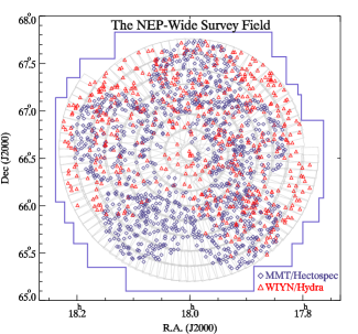
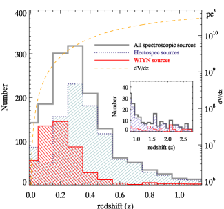
Figure 1: Left panel shows the spatial distribution of the sources observed by follow-up spectroscopic surveys over the NEP-Wide field. The centre of this map is the North Ecliptic Pole ($\alpha=18^{h}00^{m}00^{s}$, $\delta=+66^{\circ}33^{{}^{\prime}}38^{{}^{\prime\prime}}$). Background gray boxes represent 446 pointed observation of IRC towards this field. Right panel shows the number of sources as a function of redshift. The blue colour indicates the spectroscopic targets observed using Hectospec, and the red colour shows the sources observed using WIYN. Also shown with yellow curve is $dV_{z}/dz$ in arbitrary units.

One of the advantages of using the NEP-Wide data is that we have many ancillary data sets such as high-quality optical data obtained with the MegaCam of 3.5m CFHT (Hwang et al. 2007) and the 4k $\times$ 4k SNUCAM (Im et al. 2010) of the 1.5m telescope at Maidanak observatory in Uzbekistan (Jeon et al. 2010). In addition, near-IR $J-$, $H-$ band data have been obtained (Jeon et al. 2014) using the FLoridA Multi-object Imaging Near-ir Grism Observational Spectrometer (FLAMINGOS; Elston et al. 2006) mounted at the Kitt Peak National Observatory (KPNO) 2.1m telescope, and various radio data over a limited region (Kollgaard et al. 1994, Lacy et al. 1995, Sedgwick et al. 2009, White et al. 2010). Recently, the Herschel Space Observatory (Pilbratt et al., 2010) covered the entire AKARI NEP-Wide field with the Spectral and Photometric Imaging Receiver (SPIRE; Griffin et al. 2010).

For the IR sources detected by AKARI NEP-Wide survey, all the photometry results of IRC bands as well as ancillary data were produced in the form of (optical to MIR) band-merged catalogue covering $u^{*}$ band to 24 $\mu$m band (Kim et al. 2012). To construct a reliable source catalogue, all of the detected sources at one AKARI/IRC band were cross-matched with those in the other IRC bands and all the ancillary data sets including optical (CFHT and Maidanak) and FLAMINGOS near-IR bands ($J$ and $H$). The catalog contains about 114,800 sources detected at least in one of the IRC filter bands. No attempt to distinguish the sources into different types such as stars, galaxies has been made yet systematically for the entire sources in this NEP-Wide Catalogue. However, we inspected sub-sample of NEP sources based on various colour-colour diagrams with the stellarity parameters of optical counterparts, and assessed that about 70% of the MIR sources (with $S11$ magnitude brighter than 18.5 mag) are star-forming galaxies mostly at redshift range z $<$ 1 (see Lee et al. 2007; Lee et al. 2009; Kim et al. 2012). The active galactic nuclei (AGNs) and early-type galaxies comprise approximately 10% or more among the sample we inspected. The rest of them are most likely galactic stars. We expect that the composition of entire MIR sources in the NEP-Wide catalogue should be similar.

2.2 Spectroscopic Data and Galaxy sample

Follow-up spectroscopic surveys over the entire AKARI NEP-Wide field were carried out with MMT/Hectospec and WIYN/Hydra (Shim et al. 2013). The targets for spectroscopic follow-up observation were selected primarily based on MIR fluxes at 11 $\mu$m ($<$ 18.5 mag, or $f_{S11}>$ 150 $\mu$Jy) and at 15 $\mu$m ($<$ 17.9 mag, or $f_{L15}>$ 250 $\mu$Jy). An additional $R$-band magnitude cut was imposed to select optically bright objects ($16<R<21$ for Hydra, $16<R<22.5$ for Hectospec observations) that can yield the spectra with reasonable signal-to-noise (S/N) ratio. Most of these flux-limited targets are considered to be various types of IR luminous star-forming galaxies. In addition to these primary targets, a smaller number of secondary targets were selected using their optical colours ($g-r$, $B-R$, etc.) and IRC band colours ($N2-N4$, $S7-S11$). These secondary criteria include high-redshift galaxy candidates based on dropout techniques ($u$-dropout for $z\sim$ 3 and $g-$ or $B-$dropouts for z $\sim$ 4), active galactic nuclei (AGN) candidates selected by the NIR ($N2-N4>0$) and MIR ($S7-S11>0$) colours reflecting power-law SED of an AGN (e.g., Lee et al. 2007), radio sources (White et al. 2010), polycyclic aromatic hydrocarbon (PAH)-luminous galaxies (Ohyama et al.,2009; Takagi et al., 2010), and so on. The supercluster member candidates in the NEP field at z $=$ 0.087 (Ko et al. 2012) were included in the targets for this spectroscopic observation. Majority of the secondary targets are not used in the analysis for the LF derivation because they are cluster members or at $z>0.3$.

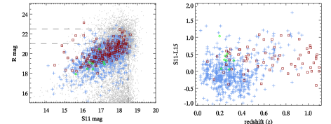
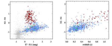
Figure 2: The upper left panel shows the distribution of spectroscopic sample in optical $R$ band versus MIR $S11$ band magnitudes plane, together with the primary selection criteria from $S11$ band and additional $R$-band magnitude cut for spectroscopic observations. Upper right panel shows the distribution of $S11-L15$ colour as a function of redshift. Lower left panel is an near- and mid-infrared colour-colour diagram showing photometric properties of the spectroscopic sample, and lower right panel shows the NIR colour distribution as a function of redshift. Backgroundnd gray dots represent parent photometric sample, and cross indicates sample classified as ‘galaxy’. Square and diamond indicate those classified as type-1 and type-2 AGNs, respectively.

Shim et al. (2013) presented spectra of 1796 sources (primary targets: 1155, secondary targets: 641), among which spectroscopic redshifts are measured for 1645 objects. The success rate for redshifts identification are higher than 80% at R $<$ 21 mag, though the quality of the spectra varies significantly depending on the targets in different fields. Quality flag ranging from 1 to 4 was assigned to each source: 4 for a secure redshift, 3 for an acceptable and almost good redshift, 2 for a questionable, and 1 for unusable redshift. We did not use the sources having the flag 1 or 2 ($\sim$ 190). The spectroscopic redshifts of $\sim$ 90% of the sources are distributed over the redshift range of z $<$ 1.0 (120 sources out of these are galactic stars), and the remaining 10% lie at z $>$ 1.0. Due to the target selection seeking for high-redshift AGNs, most sources at z $>$ 1.0 are Type-1 AGNs. Details of the line flux measurements and diagnostic line ratios can be found in Shim et al. (2013). The spatial distribution of the NEP-Wide sources observed by this spectroscopic survey is presented in the left panel of Figure 1 along with the NEP-Wide survey area. The blue diamonds indicate the spectroscopic targets observed with MMT/Hectospec, and the red triangles show the targets observed with WIYN/Hydra. We also show the redshift distribution of this spectroscopic sample in the right panel of Figure 1. All the spectroscopic sources are shown in black colour. The blue line indicates the distribution of sample observed with MMT/Hectospec, and the red one represents that observed with WIYN/Hydra. Also shown with a yellow curve is the shape of $dV_{z}/dz$, where $V_{z}$ is the comoving volume within redshift $z$. It is clear that our spectroscopic sample seriously underrepresents the galaxies beyond $z>0.35$, but is consistent with constant spatial density below $z<0.35$. We used the sample at $z<0.3$, where the spectroscopic incompleteness is less severe. The redshift distribution of the sources with higher redshifts ($>1$) is shown in an inner small box.

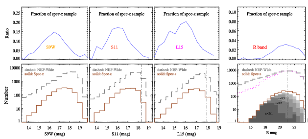
Figure 3: Upper panels show the fraction of spectroscopic sample relative to the photometric sources as a function of observed magnitudes at the MIR bands of AKARI ($S9W$, $S11$, and $L15$) and optical R band (the rightmost panels). In the lower panels, dashed line indicates the number of parent photometric sources and solid line indicates the spectroscopic sample. Dotted line in the rightmost panel indicates the sources except for the stars. Vertical dot-dashed lines indicate magnitude cut used for the target selection.

In Figure 2, we present the IR properties of the parent photometric sources and spectroscopic sample used in this work. Using analysis of emission line fluxes, Shim et al. (2013) identified the types of spectroscopic sources. They presented Baldwin-Phillips-Terlevich (BPT) diagram for the sources using emission lines ratios such as [O III]/H$\beta$ and [NII]/H$\alpha$, and classified them into star-forming galaxies, starburst-AGN composites, and AGNs. The sources classified as ‘galaxy’ are indicated by crosses (blue colour) while those classified as ‘AGN’ types are indicated by small boxes (squares for type-1 and diamonds for type-2), whose types are identified based on the analysis of emission lines (Shim et al. 2013). In the upper left panel of Figure 2, we give the distribution of the optical ($R$) versus MIR ($S11$) band magnitudes of the NEP-Wide sources, together with the primary criteria from $S11$ band and additional $R$-band magnitude cut for the spectroscopy. The background gray dots indicate parent photometric sources from the NEP-Wide catalogue. Upper right panel shows the distribution of MIR-band colour $S11-L15$ as a function of redshift, showing most of the galaxy sample gathered between -0.5 and 0.5 in this colour range with the redshift $z<0.5$, compared to the wider spread of the AGN types. In the lower left panel, the colour-colour diagram of the AKARI NIR and MIR bands shows that the sources classified as AGNs are clearly distinguished by the relatively red NIR colour ($N2-N4$) and narrow range of MIR colour ($S7-S11$). The sources classified as ‘galaxy’ are mostly distributed in the range of $-1<N2-N4<0$. The lower right panel shows the $N2-N4$ colour as a function of redshift. Figure 2 shows that MIR colours are efficient tool which can be used to demarcate between galaxies and AGNs. Especially, the ‘galaxies’ types (which we use in this work) are gathered at lower (mostly $z<0.5$) redshifts and in a narrow range of NIR colour ($-1<N2-N4<0$), while having a wider distribution in the MIR colour domains ($S7-S11$ and $S11-L15$) suggesting the various kinds of spectral energy distributions (SEDs) in the MIR wavelengths. Also, there exist intriguing sources such as those classified as ‘galaxy’ but having red NIR colour (e.g., $N2-N4>0$), which we should investigate further later when we classify entire sources in the NEP-Wide catalogue.

In Figure 3, the number distributions of the entire photometric (dashed) and spectroscopic sample (solid) are shown in the bottom panels while the ratio of the spectroscopic sample is shown in the upper panels, as a function of observed MIR bands ($S9W$, $S11$, and $L15$) and optical $R$-band (the rightmost panel) magnitudes. The fraction of spectroscopic sample varies over the MIR magnitudes, and shows broad peaks at around 16 (15.5 – 16.5) magnitudes (AB). Since the number of sources in optical band is much larger than those in the MIR bands, the fraction at $R$-band is much lower than in the MIR bands. In the lower right panel, a dotted line represents the distribution of R-band sources except for the star-like sources defined by the criteria based on the optical mag and NIR colours (Jeon et al. 2010; Kim et al. 2012; Jeon et al. 2014). For the spectroscopic sample, the variation from the darkest to brighter shades show relative amount of sample at the redshift bin $0.0<z<0.1$, $0.1<z<0.2$, $0.2<z<0.3$, and so on. Vertical dot-dashed lines indicate the magnitude cuts used for the spectroscopic target selection. There are many sources fainter than this criteria due to the deeper limit of the Hectospec. The incompleteness is more significant at higher redshift bin. Our limitation of the redshift range ($z<0.3$) effectively minimize the incompleteness arising from the flux limited sample by the magnitude cuts.

2.3 SED Fitting

Galaxy emission in the MIR is the sum of the Rayleigh-Jeans tail of stellar emission, emission from heated dust, and a power-law component of AGN, if it exists. Since our interest is to investigate the star-forming activity and to construct their LFs, we have to know the type of IR sources and classify them into galaxies or AGNs. Shim et al. (2013) identified the types of spectroscopic sources and classified them into star-forming galaxies, starburst-AGN composites, and AGNs based on the line analysis. For this work, we adopted sample classified as ‘galaxy’ having reliable spectroscopic redshift. After excluding AGNs and unreliable spectroscopic redshift, we have 1090 galaxies. By limiting the redshift range of galaxies to $z<0.3$ to construct the local luminosity functions, we are left with about $\sim$ 600 galaxies.

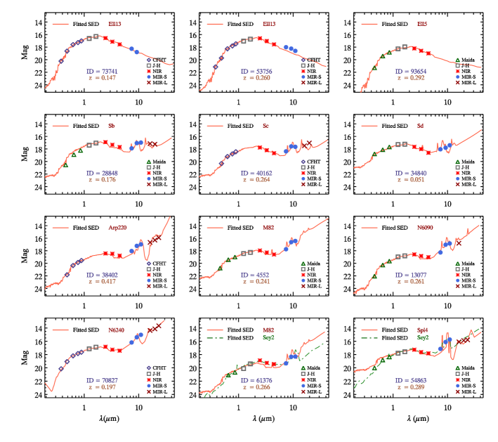
Figure 4: Examples of SED-fitting results for our sample. The horizontal axis is observed wavelength and the vertical axis is observed magnitudes (AB). The small squares indicate available photometric data points from $u$, $g$, $r$, $i$, $z$ (CFHT: diamonds), $B$, $R$, $I$ (Maidanak: triangles), $J$, $H$ (KPNO: squares), $N2$, $N3$, $N4$ (AKARI NIR bands: asterisks), and $S7$, $S9W$, $S11$ (MIR-S: filled circles), $L15$, $L18W$, $L24$ (MIR-L: x-symples). Here we show sample galaxies fitted to various model templates (e.g., elliptical, spiral, and starburst). Red lines represent the galaxy template from Polletta (2007). In the bottom panel, two galaxies are fitted to both normal galaxies and Seyfert 2. We have chosen normal galaxy fit in such circumstances because the AGNs have been already excluded based on line diagnostics.

To estimate MIR luminosities for our sample with the spectroscopic-$z$, we carried out SED fit analysis. We utilized the publicly available code Le PHARE (Ilbert et al. 2006). The fitting to SED models was done over all the available photometric band data with the spectroscopic redshift (by an option ZFIX$=$yes). We selected an option for the Calzetti extinction law (Calzetti, 2001; Fischera et al. 2003) in the software (EXTINC_LAW$=$calzetti.dat). Details of the software are given in Ilbert et al. (2006). For each observed SED, Le PHARE carried out single fit from the $u^{*}$ to the mid-IR band, using various templates defined throughout this wavelength range (Polletta et al. 2007; Ilbert et al. 2009). We searched for a best-fit model among all types and chose a template giving a minimum $\chi^{2}$. In Figure 4, we present some of our local ($z<0.3$) galaxy sample (e.g., ID$=$ 73741, 53756, 93654, 28848, 40162, 34840, 38402, 4552, 13077, 70827, and 61376) fitted to various templates. The small squares indicate available photometric data points from $u^{*}$, $g^{\prime}$, $r^{\prime}$, $i^{\prime}$, $z^{\prime}$ (CFHT: diamonds), $B$, $R$, $I$ (Maidanak: triangles), $J$, $H$ (KPNO: squares), $N2$, $N3$ ,$N4$ (AKARI NIR bands: asterisks), $S7$, $S9W$, $S11$ (MIR-S: filled circle), and $L15$, $L18W$, $L24$ (MIR-L: x-symbols). The first row shows galaxies that are fitted to ellipticals (Ell5 and Ell13), the second row shows sample fitted to spiral galaxies (Sb, Sc, and Sd types), and the third and bottom rows show those fitted to various starburst galaxies, ULIRGs, (e.g., M82, N6090, and N6240 type) and AGN (e.g., Seyfert type 2). Some sample fits better to AGN template which gave a smaller $\chi^{2}$ than that of a best-fit galaxy template, although we used objects classified as various types of ‘galaxy’ based on the optical line analysis. In this case, both template showed similar acceptable fit over the entire data points (see the last sample presented in Figure 4). Considering rather complex MIR features and larger photometric uncertainties in the longest part of MIR bands, slight confusion between galaxies and AGNs for some sample seems inevitable. Because the SEDs from both types are very similar in the MIR, the sources fitted better to AGN types do not make significant difference in our resulting MIR LFs.

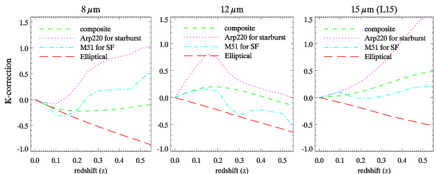
Figure 5: K-corrections for 8 $\mu$m, 12 $\mu$m, and 15 $\mu$m bands are shown. The 8$\mu$m band is strongly affected by the PAH emission features around the band widths while the NIR bands take mainly stellar emission. Therefore 8 $\mu$m bands have the model dependency and shows positive K-correctioin for starbursts and star-forming galaxies because those bands include the PAH features around 7 – 8 $\mu$m in low redshift range.

The K-correction (Oke $\&$ Sandage, 1968), which transforms the measured flux at a given wavelength to the unredshifted flux at that band, is also computed in this procedure. We checked the amount of K-corrections for the MIR bands where we derive the LFs, assuming simple box function centered at 8 and 12 $\mu$m having full-width of 2 $\mu$m and using L15 band response function. K-correction, depending on the SED of galaxy, its redshift ($z$), and the filter response ($S(\lambda)$), can be computed by

$$K(z)=(1+z)\frac{\int{F(\lambda)S(\lambda)}d\lambda}{\int{F({{\lambda}\over{1+z}})S(\lambda)d\lambda}}.\\$$ (1)

Figure 5 shows the K-corrections at 8 $\mu$m, 12 $\mu$m, and 15 $\mu$m bands for a few representative SED models from the Polleta et al. (2007). These figures show substantial differences in the K-correction behavior for different types of galaxies because the SEDs in MIR portion vary significantly depending on galaxy types. For example, the 8 $\mu$m bands show sensitive dependencies, because there are PAH features at 6.2 $\mu$m, 7.7 $\mu$m, and 8.6 $\mu$m and some of them can be included or excluded in this band depending on the redshift. In particular, 8.6 $\mu$m feature is located near the boundary of the 8 $\mu$m band, and thus can be excluded for the galaxies at low but non-zero redshift. From z $\sim$ 0.11, the 7.7 $\mu$m PAH feature begins to move out of this band. The K-correction is small but not negligible in the MIR bands for nearby galaxies. In the case of early-type galaxies, K-correction decreases monotonically with redshifts since the flux decreases with wavelength near these bands. Our sample used for this work is located at $z<0.3$ and mostly appears to be normal spiral/SF galaxies (strongly dominated by late-types), explainable with M51 type (cyan dot-dashed lines in Figure 5), while actively star forming populations such as Arp 220 (or LIRG/ULIRGs) or AGN types appear to take a very small faction.

3 Derivation of Luminosity Functions

3.1 $1/V_{max}$ Method

Luminosity function $\Phi(L)$ is the number density of galaxies having luminosity in the range $L\sim L+\Delta L$ and residing in a specific volume. Therefore, we should take a volume limited sample and count all the galaxies in a given luminosity bin and divide it by the surveyed volume. However, it is not as simple since the sample is usually limited by flux rather than volume. It means that the survey volume depends on the brightness or luminosity of the objects in the observation. In order to account for this simple fact, $1/V_{max}$ method (as described by Schmidt, 1968) is widely used to obtain the LFs of flux limited sample. This method is known to be relatively insensitive to the incompleteness of the observations, and there is no parametric dependence or assumed model. One can calculate luminosity ($L_{\nu}$) in the rest frame or absolute magnitude ($M_{\nu}$) based on a redshift and observed SED (observed magnitudes $m_{\nu}$ at each band) of each source, by following formula,

$$M_{\nu}=m_{\nu}-5~{}\log(d_{L})-25-K(z,\lambda),\\$$ (2)

where $d_{L}(z)$ is the luminosity distance (in units of Mpc) and K is $K$-correction. Using this equation, we can compute $z_{max}$, which is the maximum redshift at which a source could be observed with the detection limits of the survey (at which $m_{\nu}=$ detection limit). When converting the observed flux (or magnitude) in observed wavelength to luminosity of the rest-frame wavelength, we need to apply $K$-correction, which is calculated using the best-fit template for each source (sec. 2.2). A comoving volume $V_{max}=V(z_{max})-V(z_{min})$ associated with a source is the maximum volume corresponding to the maximum redshift within which the source could be still detected, where $z_{min}$ is the lower limit of the redshift bin. If $z_{max}$ is larger than the upper limit of the interested redshift bin (i.e., $z=0.3$), we take smaller one, i.e., $z_{max}$ = min ($z_{upper}$ of the z-bin, $z_{max}$ of a source). We estimated $z_{max}$ and $V_{max}$ at each band where we derive LFs. We collected the sources having same luminosity ranges (i.e., finite bin size, $\Delta L$). After assigning $V_{max}$ to each source, the LF($\Phi$) can be obtained by

$$\Phi(L)=\frac{1}{\Delta{L}}~{}\sum_{i}\frac{1}{V_{max,{i}}}~{}s_{i}$$ (3)

where $\Phi(L)$ is the number of objects per Mpc³ in the rest frame luminosity range $L\sim(L+\Delta L$), $s_{i}$ is correction factor to compensate the selection bias or incompleteness for $i$th galaxy, which will be described in detail in the following section 3.2.

3.2 Incompleteness and Uncertainties

Since our sample is not a complete set and has photometric uncertainties, we should take these facts into account in deriving the LFs. First, the number of galaxies with spectroscopic redshifts are much smaller than that of parent photometric sources in the NEP-Wide field, as shown in Figure 3. We compared the number distribution of the spectroscopic sample with that of entire S11 sources from the NEP-Wide catalogue as a function of magnitude to obtain the selection function for spectroscopic sample because the targets for the spectroscopic observations are selected based mainly on the S11 magnitude. In Figure 6, the orange solid line indicates all the S11 sources from the AKARI NEP-Wide survey. The gray lines show the number distribution of the sources from spectroscopic observation: from top to the bottom, all the spectroscopic sample, sample with reliable redshifts, and those classified as galaxy. The solid brown line shows the sources classified as galaxies, which are used for the estimation of LFs. The uncertainty associated with the correction for the number of the spec-z sample can be explained by the Poisson statistics in the number of the parent photometric and spectroscopic sample. It is normally a few % level at $S11>15.5$ mag (AB), but reaches around $\sim 10\%$ at $S11<15$ mag due to the smaller number of sample. This correction uncertainty appears to affect error-bar sizes of LF by several % on average ($\sim 10\%$ at most).

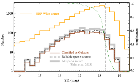
Figure 6: The number of sources as a function of observed magnitude at 11$\mu$m band (S11 band). The orange solid line represents the entire photometric sample of 11$\mu$m sources from the AKARI NEP-Wide photometric survey. The gray lines show the number distribution of the spectroscopic sample: from top to the bottom, all the spectroscopic-$z$ sources (thick white-gray) and spectroscopic sample with reliable redshifts (dot-dashed dark gray). The solid brown line shows the distribution of sample classified as ‘galaxy’ among the sample with reliable redshifts. A vertical dot-dashed line indicates the primary selection criteria for the spectroscopic observation ($\sim$ 50$\%$ completeness limit). Dotted line is the photometric incompleteness based on artificial star simulations by Kim et al. (2012).

Second, the parent photometric data becomes partially incomplete near the detection limit. At the MIR-S (S7 – S11) bands, the detection limit ranges 19.5 – 19 mag and the 50% completeness levels are $\sim$ 0.6 mag brighter than the detection limits. The magnitude difference between the 90 $\%$ and 10 $\%$ completeness is about 0.7 – 0.8 mag, indicating that the completeness begins to drop quite rapidly from around 90 $\%$ level (18.3 – 17.9 mag). We should also be careful at the bright end because the low sampling rate could derive unnatural selection function. In Figure 6, the green dotted line with the right-side vertical axis indicates the completeness level at S11 band obtained by simulation of artificial source injection and re-extraction tests as described by Kim et al. (2012). A vertical dot-dashed gray line roughly corresponds to the primary selection criteria for the spectroscopic observation (50$\%$ completeness limit of the NEP-Wide survey). We applied the correction for this photometric incompleteness based on the completeness estimation of the $S11$ data that was obtained by Kim et al. (2012) in our derivation of the LFs. There is also redshift bias as shown in the right-hand panel of Figure 1. We compared the number density of spectroscopic sources in the comoving volume corresponding to each redshift bin in order to estimate the redshift incompleteness. Assuming constant number density, we estimated the correction for incompleteness as a function of $z$. Since our derivation of LFs is limited to $z<0.3$ where the source distribution is roughly consistent with the constant spatial density, we regard the redshift bias is not significant.

Rest frame luminosity is directly derived from SED-fit results, therefore, error estimation for luminosity function (LF) depends on the SED-fitting errors arising from redshift, $k$-correction error, and photometric uncertainties. Since we used the redshifts measured by spectroscopic observation, we can ignore uncertainties from the redshifts (which is very small). Thus, our LF errors can be determined based mostly on the photometric error. In order to estimate the errors of the LFs, we carried out Monte Carlo simulation using random number generator. We generated more than 10,000 simulated catalogues by putting random errors into the measured flux of each source. In the simulated catalogues, those errors are realized by assuming a normal Gaussian distribution centered at the observed flux. Standard deviation of this gaussian distribution for simulated errors is determined based on photometry measurement error. This means we generated $\sim$ 10,000 input catalogues for Le PHARE runs doing SED-fit and obtained result sets, which finally results in slightly different 10,000 LFs. We determined final luminosity function and its uncertainties based on weighted average and the dispersion of the simulated results.

4 Results and Discussion

4.1 8 $\mu$m Luminosity Function

It is known that 8 $\mu$m luminosity of galaxy is well correlated with the total IR luminosity (Babbedge et al. 2006; Caputi et al. 2007; Bavouzet et al. 2008; Goto et al. 2010; Galametz et al. 2013) because the rest-frame 8$\mu$m fluxes are dominated by prominent PAH features which are sensitive to star formation activity. In this section, we present 8 $\mu$m luminosity function of local galaxies in the NEP-Wide field. To estimate 8$\mu$m fluxes at observed frame, we used a simple boxy filter centered at 8$\mu$m with a 2$\mu$m bandwidth across the filter (constant transmission over the bandwidth) and convolved the filter response with best-fit template for each galaxy. The observed flux and the rest-frame luminosity are related by following equation

$$L_{\nu}(\nu_{rest})=\frac{4{\pi}{D_{L}}^{2}}{(1+z)}F_{\nu}(\nu_{obs}),$$ (4)

where $D_{L}$ is the luminosity distance for a given redshift based on the cosmological parameters assumed in this work, $F_{\nu}$ the flux density (erg cm^-2 Hz^-1), and $\nu_{obs}$ and $\nu_{rest}$ are the observed and rest-frame frequencies, respectively, related by $\nu_{rest}=(1+z)\nu_{obs}$.

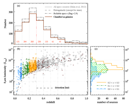
Figure 7: Top panel (a) shows the fraction of the sources which is classified as galaxies among all the spectroscopic sample as a function of redshift. Solid gray line indicates all the spectroscopic sources, dotted-dashed lines represents the sources with the reliable redshifts, and the black line shows the number of sources classified as galaxies. At the bottom, left panel (b) shows the luminosity distribution of galaxies at rest-frame 8 $\mu$m as a function of redshift. Dark red points represent sample classified as AGN. A broken curve indicates the flux limit of observation at 8 $\mu$m according to redshift. Bottom right panel (c) shows the number of galaxies with 8 $\mu$m luminosity in each redshift bin from 0.0 to 0.3. Sky-blue colour represents the sample in the redshift $z=0.0-0.1$, green colour indicates the sample in the range of $z=0.1-0.2$, and orange colour shows the sample in $z=0.2-0.3$.

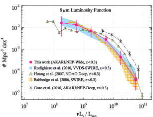
Figure 8: 8 $\mu$m luminosity functions (LFs) for local SF galaxies. The filled circle (magenta colour) represents the LF of local ($z<0.3$) galaxy sample in the NEP-Wide survey field (this work). Shaded area indicates the LF of Rodighiero et al. (2010) using VVDS-SWIRE data. Meshed region shows the results from Babbedge et al. (2006) based on the SWIRE data. Triangles are from Huang et al. (2007, NOAO deep), and ‘x’ symbols from the G10.

In Figure 7, we show the distribution of the sources used to derive 8 $\mu$m luminosity function. The top panel (Figure 7a) shows the number of sources versus redshift. The width of the redshift bin is 0.1, as indicated by vertical gray broken lines. From all the spectroscopic sample to those classified as galaxies, the amount of sample is shown by solid gray line (all spec-z sample), broken lines (except for stars and reliable spec-z), and the brown solid line (galaxies). We give the number of galaxies on histogram bar chart for each redshift bin. The bottom left panel (Figure 7b) shows the 8 $\mu$m luminosity distribution of sample as a function of redshift. The squares represent all the spectroscopic sample, but for $0<z<0.3$, the sample in each redshift bin over the detection limit is over-plotted with diamonds, triangles, and squares, respectively. The dark red dots represent those classified as AGNs, and a dashed curve indicates the luminosity corresponding to the 8 $\mu$m flux limit as a function of redshifts. The estimation of the flux limit depends on SED model, but in the range $z<0.3$, different models do not make significant changes ($\sim$ a few %). We estimated the 8 $\mu$m flux limit based on a simple flat SED. For the NEP-Wide survey, the detection limits in the mid-IR bands of IRC increases almost linearly as a function of a filter’s central wavelength. Therefore we derived detection limit at 8 $\mu$m through the interpolation. Our sample is brighter than the detection limit of S11 band, but it is not always in 8 $\mu$m band. Since 8 $\mu$m flux and luminosities are estimated from the SED-fit results, some sample can have 8 $\mu$m luminosities lower than the detection limit curve. In the bottom right panel (Figure 7c), the number distribution of these sources are shown as a function of 8$\mu$m luminosity for each redshift bin using the same colour as used in the left panel.

We constructed the 8 $\mu$m luminosity function for star-forming galaxies (at $0<z<0.3$) using the sample presented in the Figure 7c. In the redshift bin of $0<z<0.1$, a vertical clustering (Figure 7b) at around z $\sim$ 0.09 is due to the presence of a supercluster at z $=$ 0.087 in the NEP-Wide survey data. We did not include it ($\sim$ 90 sample at $0.07<z<0.1$, see Ko et al. 2012) for the estimation of luminosity function because its local over-density could affect the luminosity function. We present the 8$\mu$m luminosity function for local SF galaxies (SFG) in the NEP-Wide field in Figure 8. While a large fraction of the sample occupy $10^{9}$ – $10^{10}$ luminosity range (Figure 7c), there are too small number of sources fainter than $10^{8}L_{\odot}$. At around $z\sim 0.1$, the 8 $\mu$m detection limits according to the redshift exceeds $10^{8}L_{\odot}$ indicating many local sample fainter than $10^{8}L_{\odot}$ could not be detected in this survey. Therefore, it is hard to produce a statistically meaningful $\Phi(L)$ for this luminosity range. We compared our LF with previous results from various literatures. In Fig 8, shaded area indicates the LF from Rodighiero et al. (2010), which is based on the data from Spitzer surveys on the VIMOS VLT Deep Survey (VVDS-SWIRE) and GOODS fields. Triangles show the LF of local ($z<0.3$) galaxies in the NOAO deep field in Boötes field (Huang et al., 2007). Meshed area indicates the LF of local ($z<0.25$) galaxies in the SWIRE field from Babbege et al. (2006). These different works are summarized in Table 1. Rodighiero et al. (2007) used a library of template SEDs based on Polletta et al. (2007) and Franceschini et al. (2005). Babbedge et al. (2006) used the SED models from Rowan-Robinson et al. (2005) and photometric-redshifts. Their SFG/AGN separation is based on SED-fit results. Huang et al. (2007) used models from Lu & Hur (2000) with spectroscopic redshifts. A part of works from G10 presented here shows a LF for a higher redshift range ($0.38<z<0.58$), which was based on the NEP-Deep survey and photometric redshifts ($\sim$ 500 sample). We fit our 8 $\mu$m LF using a double -power law (Marshall 1987; Babbedge et al. 2006; Goto et al. 2010) as

$$\Phi(L){{dL}/{L^{*}}}={\Phi}^{*}\left[\left({{L}\over{L^{*}}}\right)^{1-\alpha}+\left({{L}\over{L^{*}}}\right)^{1-\beta}\right]{{dL}\over{L^{*}}}.$$ (5)

The best fit parameters for the normalization factor ($\Phi^{*}$), and the characteristic luminosity ($L^{*}$) are $2.2\times 10^{-3}$ (Mpc^-3dex${}^{-1})$ and $4.95\times 10^{9}(L_{\odot})$, respectively. We obtained the faint-end slope $\alpha=1.53$, and the bright-end slope $\beta=2.85$, which are comparable to those of the adjacent redshift bin ($0.38<z<0.58$) from G10. Our local LF spans wide luminosity ranges and is clearly shifted toward the lower density at a given luminosity in comparison with the LF from G10, indicating luminosity evolution. Our LF shows a good agreement with that of Rodighiero et al. (2010) but, in general, is consistent with other works. The difference between LFs also exist (e.g., some deviation of Huang’s). At the faintest luminosity ranges, rather larger photometric errors (with smaller number statistics if any) can count for the fluctuation. At higher luminosity ranges, it is more difficult to track down the origin of the differences in detail. But the differences seem to originate mostly from the different incompleteness in each sample and corrections for them. We regard that different number of sources contributing to each luminosity bin and AGN fraction to be excluded are also entangled and seem to affect the disagreement, even though it’s hard to compare how the individual works deal with correction factors.

4.2 Luminosity Functions for 12 $\mu$m and 15 $\mu$m

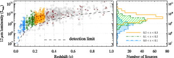
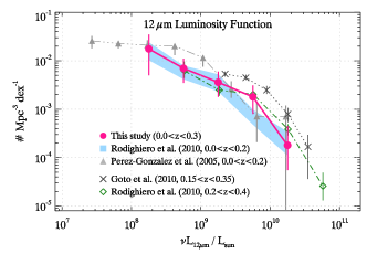
Figure 9: Top panels show 12 $\mu$m luminosity distribution of local galaxies in the NEP-Wide field as a function of redshift (left) and number of sources in each luminosity bin (right). Bottom panel shows the 12 $\mu$m luminosity function derived from the upper panels. In the bottom panel, filled circles represent this work for local ($z<0.3$) galaxies in the NEP-Wide survey field. Triangle represent the local LF derived by Pérez-González et al. (2005). Shaded area and diamonds indicate the LF for $0.0<z<0.2$ and $0.2<z<0.4$ from Rodighiero et al. (2010) using VVDS-SWIRE data. ‘x’ symbols indicate LF for galaxies at $0.15<z<0.35$ from the G10.

We construct 12 $\mu$m luminosity function (LF) of local galaxies similar way. 12$\mu$m luminosity has also been studied well based on the IRAS and ISO observations (Spinoglio et al. 1989; Rush et al. 1993). It is also known to have good correlation with total IR luminosity, and recognized as one of the indicator of galaxy SF activity. (Spinoglio et al. 1995; Pérez-González et al. 2005). The continuous wavelength coverage of our photometric data (from the near-IR) all the way through 24 $\mu$m band is very useful/helpful to obtain accurate 12 $\mu$m luminosity based on good SED fit with spectroscopic redshift. The detection limit at 12$\mu$m band corresponds to about 18.8 mag and 50% completeness level is around 18.0 mag (AB). Due to the slightly different limit and luminosity distribution from those of the 8 $\mu$m, the number of sample selected in each 12 $\mu$m luminosity bin differs a few $\%$ from that of 8 $\mu$m luminosity function (LF), as shown in the upper panels of Figure 9.

In the lower panel of Figure 9, we present our 12 $\mu$m luminosity functions (for $z<0.3$) along with other results. The filled circles (magenta) represent the LF of local ($z<0.3$) galaxies in the NEP-Wide field (this work). The shaded area (in light blue) and diamond (green) symbols represent the LFs from Rodighiero et al. (2010) based on the VVDS-SWIRE and GOODS data, for the redshift $0.0<z<0.2$ and $0.2<z<0.4$, respectively. The filled triangle indicate the LF determined by Pérez-González et al. (2005) for $0.0<z<0.2$. We also compared with the 12 $\mu$m LF derived by G10 for galaxies at $0.15<z<0.35$ from the NEP-Deep data. The redshift ranges from these various works are partly overlapped with each other, but the filled circles, triangles and shade area represent the LFs for the local universe, while the diamond and cross symbols correspond to the LFs of higher redshift ranges. Our result (filled circles) for local galaxies agrees well with the Rodighiero’s local LF, except for a deviated point at the luminosity bin $9.5<\log{\nu}L_{\nu(12{\mu}m)}<10$, seemingly due to the different redshift ranges. For the higher-z LFs, the redshift range $0.2<z<0.4$ (diamonds) of Rodighiero et al. (2010) is slightly higher than that from G10 ($0.15<z<0.35$), but their LF is systematically lower than that of Goto et al. (2010). Both works are based on the photometric redshifts, thereby seem to contain the inevitable uncertainties. Besides, due to the samplings by different redshift bins, probably leading the different correction schemes for each incompleteness/bias might have caused the deviation from each other. However, the measurements of LFs for both fields (the NEP and the VVDS-SWIRE field) consistently suggest the evolution of 12$\mu$m LF.

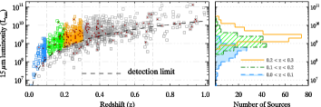
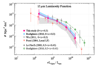
Figure 10: Top panels show 15 $\mu$m luminosity distribution of local SF galaxies in the NEP-Wide field as a function of redshift and number of sources in each luminosity bin. Bottom panel shows the 15 $\mu$m luminosity function derived from the upper panels. In the bottom panel, the circles (magenta colour) represent the LF of our ($z<0.3$) sample in the NEP field. Triangles indicate the local LF from Pozzi et al. (2004), and shaded area indicates the local LF from Rodighiero et al. (2010). Meshed region represents the results given by Wu et al. (2011). Also local LF from Le Floc’h (2005) was presented by crosses.

We also derive 15$\mu$m luminosity function of local ($0.0<z<0.3$) galaxies in the NEP-Wide field and compare with various other results. We used the same galaxy sample as used for the 8 $\mu$m and 12 $\mu$m LF, but slight different number of sample contributes to each luminosity bin (see Figure 10). While the observed magnitudes (or fluxes) at 8 $\mu$m and 12 $\mu$m bands derived from the assumed simple boxy filters with fitted SED templates, the observed 15 $\mu$m fluxes used in this section were based on the measurement by L15 filter of IRC. The 15$\mu$m LF was needed for interpretation of 15$\mu$m source properties (Xu, 2000; Gruppioni et al., 2005) since MIR observations by ISOCAM, its significance as an indicator to estimate the star formation activity has also been recognized. Since Xu et al. (2000) derived local ($z<0.2$) luminosity function based on ISOCAM 15$\mu$m observation on the IRAS 60$\mu$m galaxies ($\sim$100 sample) in the NEP region, various determination of 15$\mu$m LF has been carried out. We present the 15 $\mu$m luminosity distribution of our sample and the resulting LF in Figure 10 in comparison with several previous works. Here, the filled circles (magenta) represent our results ($z<0.3$). Pozzi et al. (2004) determined the local ($0<z<0.2$ and $0.2<z<0.4$) 15$\mu$m luminosity function using about 150 sample from the European Large Area ISO Survey (ELAIS) southern (S1: 2^∘$\times$ 2^∘, S2: $21^{\prime}\times 21^{\prime}$ ) field, based on the SED analysis mainly on M51 and M81 types as reference templates. They did not include active galaxies like Arp 220 ($L_{IR}>10^{11}L_{\odot}$) considering that those types are rare and tend to appear at higher-z (e.g., $z>0.8$). This aspect seems consistent with our local spectroscopic sample but we used many types of normal galaxy templates in the SED fit analysis. Wu et al. (2011) determined the LF for the redshift range of $z<0.3$ based on the galaxies ($\sim$ 230) from the 5 Milijansky Unbiased Extragalactic Survey (5MUSES), with the redshifts measured by Infrared Spectrograph (IRS). Their LF is also presented by meshed area in Figure 10. There is no 15$\mu$m LF measurement for the higher redshift from the NEP-Deep data. But the LFs from Le Floc’h et al. (2005) and Rodighiero et al. (2010) indicated by cross and diamond represent higher-z ($0.3<z<0.45$) LFs . Here, Le Floc’h et al (2005) used Spitzer MIPS 24$\mu$m selection at CDF-S field (0.6 deg²), carrying out analysis about 2600 sample based on both spectroscopic and photometric data from literatures and COMBO-17. These various works are also summarized in Table 1.

Table 1: Summary table showing LFs from a number of different works.

LF works	Survey Field	Size of area	Band	Nsource		Redshift info
(authors)		[deg2]	[$\mu$m]			(range)	(spec or phot)
This work	NEP-Wide	$\sim 5.4$	8, 12, 15	$\sim~{}600$		$z<0.3$	spec-z
Babbedge et al. (2006)	ELAIS N1	$\sim 6.5$	8	$\sim 5,000$		$z<0.25$	phot-z
Huang et al. (2007)	NOAO Deep	$\sim 6.8$	8	$\sim 2,600$		$z<0.3$	spec-z
Rodighiero et al. (2010)	VVDS-SWIRE	$\sim 0.9$	8, 12, 15	$\sim 440$		$z<0.3$	phot-z
Pérez-González et al. (2005)	CDFS/HDFN	$\sim 0.5$	12	$\sim 500$		$z<0.2$	phot-z
Pozzi et al. (2005)	ELAIS South	$\sim 0.5$	15	$\sim 150$		$z<0.2$	spec-z
Wu et al. (2011)	5 MUSES	$\sim 40.$	15	$\sim 230$		$z<0.3$	spec-z
Goto et al. (2010)	NEP-Deep	$\sim 0.6$	8, 12	$\sim 500$		$0.2<z<0.6$	phot-z
Rodighiero et al. (2010)	VVDS-SWIRE	$\sim 0.9$	12, 15	$\sim 300$		$0.3<z<0.45$	phot-z
Le Floc’h et al. (2005 )	CDFS	$\sim 0.6$	15	$\sim 2,600$		$0.3<z<0.45$	phot-z

5 SUMMARY AND CONCLUSION

We presented mid-infrared luminosity functions for the galaxies in the local universe. We used the sample from the NEP-Wide survey data observed by AKARI space telescope, which covered the near- to mid-IR (2 $\sim$ 25 $\mu$m) wavelengths continuously. To obtain more accurate luminosity functions, we took advantage of the spectroscopic redshift information obtained by optical follow-up surveys carried out with the MMT/Hectospec and WIYN/Hydra as well as various ancillary data sets covering from optical u^∗ to NIR $H$ band. Therefore the SED-fit analysis to determine the rest frame luminosities at MIR bands does not have serious source of uncertainties. For better statistics and completeness, we limited this study to the lower redshifts ($z<0.3$) range. Our sample appears to be composed of various types of local SF galaxies including a small fraction of ellipticals and normal galaxies with some of these having similar SEDs to those of active galaxies. For the purpose of this work to derive the MIR luminosity functions at the 8, 12, and 15 $\mu$m bands, we employed the $1/V_{max}$ method, which is widely accepted because of its merits as described in sec. 3.1.

The LFs appear to be consistent with other previous studies, in general, within error bars although the differences among various determinations seem to originate from different method for source classification/selection and different photometric data and SED models, different redshift measurements and redshift ranges of sample, different correction methods for incompleteness or selection effect, different fields/areal coverage, and so on. Errors also arises from those components. But, compared to the other works, the advantage of this work is the redshift information determined by spectroscopic observation and source classification based on line analyses as well as extensive wavelength coverage from optical u^∗ to MIR 25 $\mu$m including the AKARI’s continuous filter coverage in the MIR wavelengths, which allow us to obtain good SED-fit without large uncertainties such as those from photometric redshifts or type decision by colours or SED fit. Also, since our sample is distributed over the large area of 5.4 $deg^{2}$, our results are not susceptible to the statistical uncertainty arising from the observation on a small part of the sky. While AKARI data do not drastically change earlier results, we can give more accurate luminosity function for the luminosity ranges 10⁸ – 10¹⁰ L_⊙. Although it is not easy to say about evolution based on this work alone, valuable comparisons are possible with the higher-z LFs from the NEP-Deep survey which is complementary to NEP-Wide or various LFs of similar redshifts. The purpose of this work was achieved but exact measurements for more fainter luminosity bins and faint end slope seem to be pending. We expect to extend this study to the FIR wavelengths range and to higher redshifts using much larger number of sample than those used in this work, if we can measure photometric redshifts for the sources in the NEP-Wide catalogue.

References

- Babbedge et al. (2006) Babbedge T. S. R. et al., 2006, MNRAS, 370, 1159
- Bavouzet et al. (2008) Bavouzet N. et al., 2008, A&A, 479, 83
- Calzetti (2001) Calzetti D., 2001, PASP, 113, 1449
- Caputi et al. (2007) Caputi K. I. et al., 2007, ApJ, 660, 97
- Clements (2001) Clements D. L., et al., 2001 MNRAS, 325, 665
- Elbaz (1999) Elbaz D. et al., 1999, A&A, 351, L37
- Elston (2006) Elston R. J. et al., 2006, ApJ, 639, 816
- Fang (1998) Fang F., et al., 1998, ApJ, 500, 693
- Fischera (2003) Fischera J., et al., 2003, ApJ, 599, L21
- Franceschini (1988) Franceschini A., et al., 1988, MNRAS, 233, 175
- Franceschini (2005) Franceschini A., et al., 2005, AJ, 129, 2074
- Galametz et al. (2013) Glametz M. et al., 2013, MNRAS, 431, 1956
- Goto et al. (2010) Goto T. et al., 2010, A&A, 514, A6
- Goto et al. (2011) Goto T. et al., 2011, MNRAS, 414, 1903
- Goto et al. (2015) Goto T. et al., 2015, MNRAS, accepted
- Griffin et al. (2010) Griffin M. J. et al., 2010, A&A, 518, L3
- Gruppioni et al. (2005) Gruppioni C. et al., 2005, ApJ, 618, L9
- Hacking and Houck (1987) Hacking P., Houck J. R. 1987, APJS, 63, 311
- Hwang, N., et al. (2007) Hwang N. et al., 2007, ApJS, 172, 583
- Huang, J.-S., et al. (2007) Huang, J.-S. et al., 2007, ApJ, 664, 840
- Ilbert et al. (2006) Ilbert O. et al., 2006, A&A, 457, 841
- Ilbert et al. (2009) Ilbert O. et al., 2009, ApJ, 690, 1236
- Im et al. (2010) Im, M. et al., 2010, J. Korean Astron. Soc., 43, 75
- Jarrett et al. (2011) Jarrett T. H. et al., 2011, ApJ, 735, 112
- Jeon et al. (2010) Jeon Y. et al., 2010, ApJS, 190, 166
- Jeon et al. (2014) Jeon Y. et al., 2014, ApJS, 214, 20
- Kim et al. (2012) Kim S. J. et al., 2012, A&A, 548, A29
- Ko et al. (2012) Ko J. et al., 2012, ApJS, 745, 181
- Kollgaard et al. (1994) Kollgaard R. I. et al., 1994, ApJS, 93, 145
- Lacy et al. (1995) Lacy M. et al., 1995, MNRAS, 59, S529
- Lagache et al. (1999) Lagache G. et al., 1999, A&A, 344, 322
- Lee et al. (2007) Lee H. M. et al., 2007, PASJ, 59, S529
- Lee et al. (2009) Lee H. M. et al., 2009, PASJ, 61, 375
- Le floc’h et al. (2005) Le Floc’h E. et al. 2005, ApJ, 632, 169
- Magnellil et al. (2011) Magnelli B. et al., 2011, A&A, 528, A35
- Marshall et al. (1987) Marshall H. L., 1987, AJ, 94, 628
- Matsuhara et al. (2006) Matsuhara H. et al., 2006, PASJ, 58, 673
- Murakami, H., et al. (2007) Murakami H. et al., 2007, PASJ, 59, S269
- Ohyama et al. (2009) Ohyama Y., et al., 2009, ASPC, 418, 329
- Oke & Sandage (1968) Oke J. B., Sandage A., 1968, ApJ, 154, 210
- Onaka et al. (2007) Onaka T. et al., 2007, PASJ, 59, S401