Modularity and the spread of perturbations in complex dynamical systems

Abstract

We propose a method to decompose dynamical systems based on the idea that modules constrain the spread of perturbations. We find partitions of system variables that maximize ‘perturbation modularity’, defined as the autocovariance of coarse-grained perturbed trajectories. The measure effectively separates the fast intramodular from the slow intermodular dynamics of perturbation spreading (in this respect, it is a generalization of the ‘Markov stability’ method of network community detection). Our approach captures variation of modular organization across different system states, time scales, and in response to different kinds of perturbations: aspects of modularity which are all relevant to real-world dynamical systems. It offers a principled alternative to detecting communities in networks of statistical dependencies between system variables (e.g., ‘relevance networks’ or ‘functional networks’). Using coupled logistic maps, we demonstrate that the method uncovers hierarchical modular organization planted in a system’s coupling matrix. Additionally, in homogeneously-coupled map lattices, it identifies the presence of self-organized modularity that depends on the initial state, dynamical parameters, and type of perturbations. Our approach offers a powerful tool for exploring the modular organization of complex dynamical systems.

Many complex systems are modular, in that their components are organized in tightly-integrated subsystems that are weakly coupled to one another. Modularity has been argued to play many important roles, including increasing robustness Simon (1962); Kitano (2004); Wu et al. (2009), evolvability Simon (1962); Wagner and Altenberg (1996), and functional differentiation Tononi et al. (1994); Wagner et al. (2007). Thus, there is great interest in measures of modularity and methods for decomposing complex systems into weakly coupled modules.

This problem is here considered in the domain of multivariate dynamics, a common formalism for modeling complex physical, biological, neural, and social systems. We propose a method of identifying dynamical modules motivated by the intuition that, in a modular system, the spread of perturbations is characterized by two time scales: fast spreading within modules and slow spreading between modules Simon (1962); Pan and Sinha (2009). In our treatment, the spreading process is coarse-grained relative to a partition (a decomposition of system variables into disjoint subsystems) by measuring the magnitude of the perturbation’s effect within each subsystem over time. If a partition reflects underlying modular structure, initially perturbed subsystems remain affected as dynamics unfold, while initially unperturbed subsystems remain largely unaffected. In this case, the partition’s coarse graining will capture the slow component of perturbation spreading dynamics, an effect quantified using a quality function called perturbation modularity. Our perturbation-based approach is related to many existing techniques for analyzing multivariate dynamics, including Lyapunov-exponent based methods Luque and Solé (2000); Pomerance et al. (2009); Strogatz (2014) and impulse response analysis Koop et al. (1996).

As will be elaborated below, our methodology can identify the dependence of optimal decompositions on initial states, time scales, and kinds of perturbations applied. These factors are all important aspects of modular organization in real-world dynamical systems. Dependence on the initial condition reflects that dynamical systems can exhibit different modular organizations in different regions of their state-space; for example, distributed regions of the brain can couple into modular assemblies via oscillatory synchronization, with the same region participating in different assemblies depending on brain state Fries (2005); Womelsdorf et al. (2007). The choice of time scale affects optimal decompositions by determining the separation between intramodular and intermodular perturbation spreading; in real-world complex systems, longer time scales have often been argued to correspond to larger-scale modules Simon (1962); Wu and Loucks (1995); Arenas et al. (2006); Palla et al. (2007); Bassett et al. (2011). Finally, the dependence on the kinds of perturbations reflects that a dynamical system may be robust to some perturbations but highly-sensitive to others Carlson and Doyle (2002); for example, in biological double-knockout experiments, cellular responses to the simultaneous deactivation of two genes can differ dramatically from responses to the individual deactivation of either gene Deutscher et al. (2008).

Our approach starts from a pre-specified dynamical system and thus differs fundamentally from existing treatments of modularity based on network representations of a system. Such methods are usually unable to capture the variation of modular organization across state-space or time scale, as well as other important dynamical aspects of modularity.

For instance, one standard approach applies graph-based community detection Fortunato (2010) to the structural network underlying a dynamical process (e.g., the social network over which an epidemic spreads). This treatment ignores the fact that the same structural network can support many different dynamical processes (for example, ‘complex contagion’ epidemics proceed differently from ‘simple contagion’ epidemics Centola and Macy (2007)). In contrast, our methodology is by definition sensitive to dynamical differences.

Another class of methods detects community structure in network representations of dynamics, defined either in terms of causal interactions or statistical dependencies between variables (e.g., relevance networks in systems biology Zhang and Horvath (2005) and functional networks in neuroscience Rubinov and Sporns (2010)). Unfortunately, constructing such networks involves a conversion of the dynamical system (defined in terms of transitions between multidimensional states) into a graph (defined in terms of nodes and edges). This conversion can affect modular decompositions in opaque ways as well as invalidate presumed graph-theoretic null models Zalesky et al. (2012); MacMahon and Garlaschelli (2015); statistical dependency networks in particular require a number of nontrivial decisions regarding the choice of dependency measure (correlation, transfer entropy, phase-locking measures, etc.), treatment of positive versus negative interactions, and thresholding Rubinov and Sporns (2010). Furthermore, coupling between variables does not necessarily give rise to large values of correlation or other dependency measures Soriano et al. (2012) (also as shown in our first example below). Finally, community detection on dependency networks optimizes quality functions that are difficult to interpret in terms of the original system dynamics. Perturbation modularity does not require the construction of a network representation of a dynamical system and is interpretable in terms of the separation of slow and fast time scales of perturbation spreading.

Because our approach is based on intrinsic system dynamics, it also differs from methods that identify modules by imposing a dynamical process onto a given network, such as diffusion of random walkers Rosvall and Bergstrom (2008); Delvenne et al. (2010) or coupled phase oscillators Arenas et al. (2006); Boccaletti et al. (2007). However, as we discuss below, in certain cases our approach has connections to such methods. In particular, it can be seen as a generalization of the random-walk-based approach of Markov stability Delvenne et al. (2010); Lambiotte et al. (2014) to a broad class of dynamics.

To formally define perturbation modularity, consider a dynamical system with an $N$-dimensional state-space $\bm{X}$ and evolution operator $f^{t}:\bm{X}\rightarrow\bm{X}$ at time scale $t$ (both state and time can be continuous or discrete). Given a set $\mathcal{E}$ of possible initial perturbations, $\bm{\varepsilon}\in\mathcal{E}$ is applied to an initial condition $\bm{x}\in\bm{X}$ to produce a perturbed initial condition $\bm{x}+\bm{\varepsilon}\in\bm{X}$. After time $t$, the size of the perturbation in the whole system is measured as the norm of the difference between the perturbed and unperturbed trajectories: $\left\|f^{t}(\bm{x}+\bm{\varepsilon})-f^{t}(\bm{x})\right\|$. The relative size of the perturbation within a subsystem $S$ (a subset of system variables) is:

$$m_{S}^{t}(\bm{x},\bm{\varepsilon})=\frac{\left\|\left(f^{t}(\bm{x}+\bm{\varepsilon})-f^{t}(\bm{x})\right)_{S}\right\|}{\left\|f^{t}(\bm{x}+\bm{\varepsilon})-f^{t}(\bm{x})\right\|}$$ (1)

where the subscript $S$ on the right hand side indicates a projection onto the dimensions indexed by $S$. For simplicity, we consider only cases where the system’s perturbed and unperturbed trajectories have not merged ($\left\|f^{t}(\bm{x}+\bm{\varepsilon})-f^{t}(\bm{x})\right\|>0$) and Eq. (1) is well-defined.

Assume a partition of the system $\pi=\left\{S_{1},\dots,S_{K}\right\}$ into $K$ disjoint subsystems. The coarse-grained perturbation vector $\bm{y}_{\pi}^{t}(\bm{x},\bm{\varepsilon})=\left\langle m_{S_{1}}^{t}(\bm{x},\bm{\varepsilon}),\dots,m_{S_{K}}^{t}(\bm{x},\bm{\varepsilon})\right\rangle$ captures the relative size of the perturbation in each subsystem. Due to the normalization in Eq. (1), $\bm{y}_{\pi}^{t}$ is invariant to the dynamical expansion of the whole-system phase-space, instead reflecting only the relative effects of perturbations on different subsystems.

We now define perturbation modularity $Q^{t}(\pi,\bm{x})$ as the vector autocovariance of the coarse-grained perturbation vector:

$$Q^{t}(\pi,\bm{x})=$$ (2)

$$\;\;\;\;\textrm{E}\!\left[\bm{y}_{\pi}^{0}(\bm{x},\bm{\varepsilon})\cdot\bm{y}_{\pi}^{t}(\bm{x},\bm{\varepsilon})\right]-\mathbb{\textrm{E}}\!\left[\bm{y}_{\pi}^{0}(\bm{x},\bm{\varepsilon})\right]\cdot\textrm{E}\!\left[\bm{y}_{\pi}^{t}(\bm{x},\bm{\varepsilon})\right]$$

where the expected values are taken over $P(\bm{\varepsilon})$, a probability distribution over perturbations (i.e. the elements of $\mathcal{E}$). The first term of Eq. (2) measures the degree to which perturbations persist within a partition’s subsystems (i.e. initially perturbed subsystems remain affected after time $t$, while initially unperturbed subsystems remain relatively unaffected). The second term of Eq. (2) provides a baseline expectation of perturbation effects that accounts for differences in subsystem sizes.

As stated, the spread of perturbations in a modular system will be constrained by module boundaries. The optimal modular decomposition is the partition that maximizes perturbation modularity: ${\pi^{\star}=\arg\max_{\pi}Q^{t}(\pi,\bm{x})}$.

Perturbation modularity (Eq. (2)), as well as optimal modular decompositions, are state-dependent in that they are defined relative to an initial condition $\bm{x}.$ Different criteria may be used to determine the choice of this initial condition, such as dynamical importance (e.g., an equilibrium state), particular research interest, or random selection. Alternatively, the modularity of entire state-space regions, rather than individual states, can be measured as the expectation of perturbation modularity over a distribution of initial conditions (e.g., by averaging across the entire system state space). Similarly, stochastic dynamical systems can be accommodated by taking expectations over future state distributions. For simplicity, however, these extensions are not considered in the present work.

In addition to initial condition, perturbation modularity and optimal decompositions also depend on the time scale $t$, which, as mentioned, can act as a resolution parameter. When there is not a time scale of a priori interest, optimal decompositions can be identified at multiple resolutions by sweeping across a range of time scales. Finally, the measure also depends on the kinds of perturbations applied, as specified by $\mathcal{E}$ and $P(\bm{\varepsilon})$. In practice, perturbations can be selected according to domain knowledge (e.g., typically encountered environmental perturbations) or using ‘neutral’ options (e.g., small increments to single variables). In many cases, initial perturbations should be localized to a small number of variables (i.e. the elements of $\mathcal{E}$ are sparse) because the spread of perturbations is more pronounced when only a few subsystems are initially perturbed. As we will show, perturbations that simultaneously affect many variables probe the system at larger scales and uncover larger modules, providing another way to explore decompositions at multiple resolutions.

Like other temporally-localized methods Pikovsky and Politi (1998), perturbation modularity also depends on the norm used to measure perturbation magnitude. Below, the $\ell_{1}$ norm is used because it performs well and permits connections to community detection methods in graphs (see Supplemental Material for definition of $\ell_{p}$ norms).

Perturbation modularity is related to the Markov stability method of community detection in graphs, which identifies communities as subgraphs that trap random walkers Delvenne et al. (2010); Lambiotte et al. (2014). Similarly to perturbation modularity, Markov stability separates diffusion dynamics into fast intracommunity and slow intercommunity components. As shown in the Supplemental Material Note (1), perturbation modularity is equivalent to Markov stability when the system of interest exhibits diffusion dynamics, perturbations are homogenous increases to single variables, and the $\ell_{1}$ norm is used to measure perturbation magnitude. More broadly, our approach can be seen as a generalization of Markov Stability to other dynamics.

In addition, $\ell_{1}$ perturbation modularity on a dynamical system is equivalent to directed weighted Newman’s modularity Arenas et al. (2007); Leicht and Newman (2008) on a specially constructed graph (see Supplemental Material Note (1)). In this graph, nodes correspond to system variables and the edge from node $i$ to node $j$ has weight:

$$w_{ij}=\textrm{E}\!\left[m_{\{i\}}^{0}(\bm{x},\bm{\varepsilon})\thinspace m_{\{j\}}^{t}(\bm{x},\bm{\varepsilon})\right]$$

where the expectation is over $P(\bm{\varepsilon})$ and the subscripts $\{i\}$ and $\{j\}$ indicate single-variable subsystems. This mapping permits perturbation modularity to be maximized using highly efficient existing community detection algorithms (such as the Louvain method Blondel et al. (2008); Aldecoa and Marín (2014) used for the examples below; code is available online ).

Several criteria can be used to measure the quality of identified decompositions. High-quality decompositions have large perturbation modularity values (e.g., near 1 for $\ell_{1}$ or $\ell_{2}$ perturbation modularity, see Supplemental Material Note (1) for derivation of bounds on perturbation modularity). Additionally, high-quality decompositions are robust to small changes in system and optimization parameters. This can be quantified by measures of partition similarity like normalized mutual information (NMI) Danon et al. (2005), an information-theoretic measure that ranges from 0 (maximally dissimilar partitions) to 1 (identical partitions). In several of the examples below, we plot NMI similarity between optimal decompositions identified at close values of $t$; high NMI values indicate modular organization robust to small changes in time scale. Similar techniques are used in the Markov stability literature to identify time scales with robust decompositions Schaub et al. (2012).

We demonstrate our method on several examples of coupled logistic maps, nonlinear discrete-time dynamical systems that have been used to explore spatially-extended chaos and pattern formation Kaneko (1989). Assume a system of $N$ variables, with $x_{i}(t)$ indicating the state of variable $i$ at time $t$, and the transition function:

$$x_{i}(t+1)=(1-\gamma)g(x_{i}(t))+\gamma\sum_{j\neq i}\frac{k_{ji}}{d_{i}}g(x_{j}(t))$$ (3)

where $g(x)=1-\alpha x^{2}$ is the logistic map, parameter $\alpha\in[1,2]$ controls the chaoticity, parameter $\gamma\in[0,1]$ controls the coupling strength, ‘coupling matrix’ elements $k_{ji}$ determine the influence of variable $j$ on variable $i$, and $d_{i}=\sum_{j\neq i}k_{ji}$ normalizes the coupling strengths. When variables are homogeneously coupled to nearest neighbors on a 1-dimensional ring lattice, these systems are called coupled map lattices (CML) Kaneko (1989). Coupled logistic maps display a rich variety of spatiotemporal patterns in different parameter regimes due to the interplay between intervariable coupling (which ‘homogenizes’ variable states) and chaos (which injects variation into variable states).

We consider several examples of coupled logistic maps. Unless otherwise noted, perturbations consist of a uniform distribution over small increases to single variables: $\mathcal{E}=\left\{0.0001\cdot{\bf e}_{i}:i=1..N\right\}$, where $\mathbf{e}_{i}$ is the $i^{\textrm{th}}$ $N$-dimensional standard basis vector. The $\ell_{1}$ norm is used to measure perturbation size.

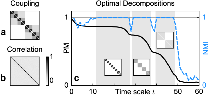
Figure 1: (Color online) System of 80 coupled logistic maps ($\alpha{=}2,\gamma{=}0.04$) (a) The coupling matrix exhibits hierarchical modularity at three levels. (b) The system is chaotic and no strong correlations between variables are observed over 10,000 time steps. (c) Perturbation modularity of optimal decompositions (PM, solid black) at different time scales $t$ and NMI between optimal decompositions at successive times (dashed blue). Three time scale regions are robust (NMI=1, grey), corresponding to the three hierarchical levels of the coupling matrix (insets).

In Example 1, we uncover modular organization that is present in a system’s coupling matrix, though not apparent in the correlation statistics. Consider an $N{=}80$ variable system with chaotic dynamics ($\alpha{=}2,\gamma{=}0.04$) and a hierarchical modular coupling matrix (Fig. 1a). The system is composed of 8 tightly-coupled low-level modules ($k_{ji}{=}1)$ with 10 variables each, pairs of which are nested within 4 mid-level modules ($k_{ji}{=}0.01)$, pairs of which are in turn nested within 2 weakly coupled high-level modules ($k_{ji}{=}0.0001)$. A random state is used as the initial condition.

Because the system is strongly chaotic for these values of $\alpha$ and $\gamma$, there is no obvious ‘order parameter’ for identifying modular organization from system trajectories Arenas et al. (2006); for instance, variable states are largely uncorrelated over 10,000 time steps (Fig. 1b). However, because perturbations first spread within low-level modules, then mid-level modules, and finally high-level modules, our method easily uncovers the hierarchical modular organization. Fig. 1c shows the perturbation modularity (black) and NMI (dashed blue) for optimal decompositions at different time scales. There are three robust time scale regions, corresponding to each of the three hierarchical levels of the coupling matrix (insets in Fig. 1c). Beyond time scale ${\sim}50$, perturbations have spread between the high-level modules; at this point, optimal decompositions reflect random fluctuations in initial conditions, and perturbation modularity and NMI values are near 0.

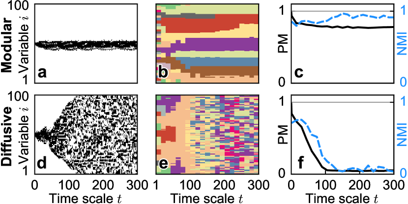
Figure 2: (Color online) Two 100-variable CMLs are compared: one ‘modular’ (top row; $\alpha{=}1.7,\gamma{=}0.1$) and one ‘diffusive’ (bottom row; $\alpha{=}1.9,\gamma{=}0.6$). (a,d) Spacetime plots of the effect of a single-variable perturbation. A pixel is colored black if the absolute difference between perturbed and unperturbed trajectory at a variable (vertical axis) exceeds 1% of the size of the system-wide perturbation at a given time (horizontal axis). (b,e) Spacetime plots of the optimal decompositions at different time scales; color indicates each variable’s subsystem. (c,f) Perturbation modularity of optimal decompositions (PM, solid black) at different time scales $t$ and NMI between optimal decompositions at successive times (dashed blue). Stable decompositions are observed in the modular CML (top row).

In Example 2, we investigate a more interesting case in which modularity emerges in a homogeneously-coupled CML. In some parameter regimes, spatial variation in initial conditions breaks the lattice coupling symmetry and leads to the emergence of modular domains (contiguous lattice regions) that constrain the spread of perturbations Kaneko (1986). Such a ‘modular’ regime is investigated using a CML with $N{=}100$ variables and weak coupling-strength ($\alpha{=}1.7,\gamma{=}0.1$). The initial condition is set by iterating a random state for 10,000 time steps. Fig. 2a shows the spacetime plot of the effect of a single-variable perturbation to this initial condition: the perturbation spreads to several nearby variables until $t{\sim}50$ but then remains confined within its domain. When computed over a uniform distribution of single-variable perturbations, our method uncovers robust modular organization for a large range of time scales (Fig. 2b), with optimal decompositions exhibiting high values of perturbation modularity and NMI (Fig. 2c).

The above system can be compared to a CML in a ‘diffusive’ regime ($\alpha{=}1.9,\gamma{=}0.6$). For these parameters, the effects of perturbations spread freely across the lattice, as shown in the spacetime plot of Fig. 2d (initial condition is the same random state as in the modular CML iterated for 10,000 time steps). This system does not exhibit robust modular organization: optimal decompositions are not stable (Fig. 2e) and optimal perturbation modularity and NMI values are low (Fig. 2f). Once the effects of perturbations spread completely around the ring lattice at $t{\sim}100$, both optimal perturbation modularity and NMI values are near $0$.

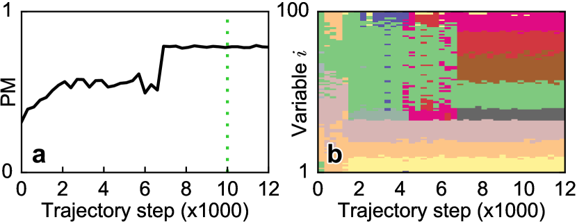
Figure 3: (Color online) State-dependence in the modular CML. For a $12,000$ step trajectory starting from a random state, optimal decompositions (time scale $t{=}300$) are identified using states along this trajectory as initial conditions. (a) Optimal perturbation modularity (PM, solid black) grows with increasing trajectory steps (horizontal axis), indicating the emergence of robust modular structures. Trajectory step $10,000$ (dotted green line) is the initial condition in examples 2 and Modularity and the spread of perturbations in complex dynamical systems. (b) Optimal decompositions identified at different trajectory steps; color indicates the subsystem of each variable (vertical axis).

In Example 3, we demonstrate state-dependent modularity by tracking the gradual emergence of modular organization over the course of a CML trajectory. The modular CML of Example 2 ($\alpha{=}1.7,\gamma{=}0.1$) was started from a random state and iterated over a $12,000$ step trajectory. The state encountered after $10,000$ time steps was previously used as the initial condition in Example 2. Here we find optimal decompositions (time scale $t{=}300$) when different states along the aforementioned trajectory are used as initial conditions. Over the course of the trajectory, optimal perturbation modularity grows through a series of plateaus (Fig. 3a), indicating the appearance of modular structures. Fig. 3b shows the optimal decompositions identified at different trajectory steps. Variables ${\sim}1{-}40$ quickly form modular structures (by trajectory step ${\sim}2000$), while variables ${\sim}40{-}100$ need almost $7,000$ steps to do so. This provides an example of self-organized modularity, or modular organization that emerges during a system’s dynamical evolution.

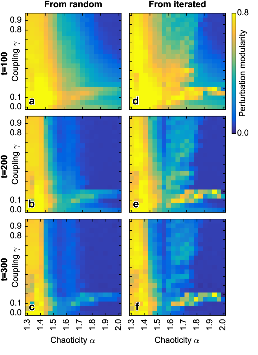
Figure 4: (Color online) Parameter phase map of CML. Perturbation modularity (color) for optimal decompositions of 100-variable CMLs with different values of chaoticity ($\alpha$; horizontal axes) and coupling strength ($\gamma$; vertical axes). Perturbation modularity is computed at three time scales for two different classes of initial conditions: random states [(a) $t{=}100$, (b) $t{=}200$, and (c) $t{=}300$] as well as random states iterated for 10,000 time steps [(d) $t{=}100$, (e) $t{=}200$, and (f) $t{=}300$].

Previously, we showed that perturbation modularity captures the presence of stable modular structures in different CML parameter regimes (Example 2), and that it can uncover modular organization in a state-dependent manner (Example 3). In Example 4, we use perturbation modularity to characterize regions in the CML parameter space with respect to the onset of modularity.

Specifically, we construct 100-variable CMLs with different values of chaoticity ($\alpha$) and coupling ($\gamma$) parameters. For these different parameter values, Fig. 4 shows optimal perturbation modularity computed at three time scales ($t{=}100$, $t{=}200$, and $t{=}300$) and two different classes of initial conditions: random states (Fig. 4a-c) and random states iterated for 10,000 time steps (Fig. 4d-f). In all cases, optimal perturbation modularity values were averaged across 10 random samples of initial conditions.

Several regimes of spatial organization can be identified in the parameter phase maps. For $\alpha\lesssim 1.44$, spatial domains, which form even when the system is started from random initial conditions, constrain the spread of perturbations over long time scales; we call this the modular regime. For other parameter values (e.g., $1.6\lesssim\alpha\lesssim 1.95$, $\gamma\sim 0.1$, the yellow ‘tongue’ in Fig. 4d-f), modular domains only appear when random states are iterated for many steps before being used as initial conditions. This regime, which includes the case studied in Example 3, we call self-organized modular. Finally, for parameter values corresponding to the blue regions in Fig. 4, which we call the diffuse regime, modular domains are not present and perturbations spread freely. Here, different parameter values give rise to different diffusion speeds Kaneko (1986): for example, $\alpha{=}1.9,\gamma{=}0.7$ exhibits no modular organization at time scale $t{=}100$; on the other hand, $\alpha{=}1.9,\gamma{=}0.2$ maintains some modularity at $t{=}100$, but this organization disintegrates by $t{=}200$.

Finally, in Example Modularity and the spread of perturbations in complex dynamical systems, we explore modularity’s dependence on the kinds of perturbations applied. We again consider the modular CML ($\alpha{=}1.7,\gamma{=}0.1$) and initial condition of Example 2. Instead of perturbing single variables, we now simultaneously perturb multiple variables in lattice-contiguous ‘windows’ of different sizes (variables simultaneously incremented by 0.0001; all $N$ windows are perturbed with uniform probability); for illustration, Fig. 5a shows the effect of a perturbation to a window of $20$ variables. Fig. 5b shows that optimal decompositions (time scale $t{=}300$) depend on perturbation size. As more variables are perturbed, smaller subsystems merge into larger subsystems in a hierarchical manner.

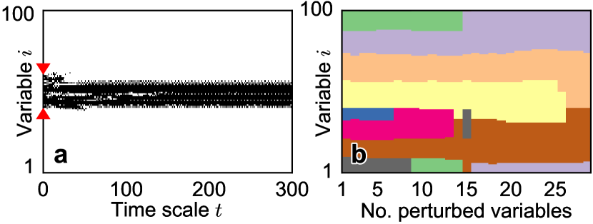
Figure 5: (Color online) Perturbation dependence in the modular CML. (a) Spacetime plot of the effect of a perturbation to a 20-variable window (red arrows), as in Fig. 2a and 2d. (b) Optimal decompositions (time scale $t{=}300$) for different perturbation sizes (horizontal axis).

Future work can pursue several extensions to our approach. First, estimating perturbation modularity from real-world datasets is of great practical interest; this can be investigated by applying the method to fitted dynamical models (e.g., vector autoregressive or dynamical causal modeling Friston et al. (2003)) or using nonparametric approaches. Second, it is possible to explore other measures of decomposition quality beyond robustness to time scale, including robustness to changes in initial conditions and kinds of perturbations; alternatively, decomposition quality may be evaluated by testing the statistical significance of optimal perturbation modularity against null-model ensembles of nonmodular dynamical systems Zalesky et al. (2012). Third, it is of interest to identify possible limitations of our method, such as whether it is susceptible to the kinds of resolution limits Fortunato and Barthélemy (2007) and detectability thresholds Nadakuditi and Newman (2012) encountered by graph-based community detection methods. Finally, future research can investigate other measures of perturbation magnitude (e.g., different norms or divergence functions), kinds of decompositions (e.g., overlapping subsystems), and cost functions (beyond vector autocovariance). For example, cost functions that capture the invertibility or sparsity of coarse-grained dynamics could be used to decompose a system into a mesoscopic ‘control diagram’, in which each subsystem controls a small number of others.

To summarize, we identify modular decompositions of multivariate dynamical systems based on the idea that modules constrain the spread of perturbations. We propose a quality function, called perturbation modularity, which can be used to identify optimal coarse grainings that capture the slow component of perturbation spreading dynamics. The method generalizes graph-based community detection to a broad class of nonlinear dynamical systems and provides a principled alternative to detecting communities in network representations of dynamics. The method captures variation in modular organization across different time scales, initial conditions, and kinds of perturbations and offers a powerful tool for exploring modularity in complex systems.

Supplemental Material

Appendix A Bounds on Perturbation Modularity

The bounds on perturbation modularity depend on the norm used to measure perturbation magnitude (see Eq. (1) in the main text). Here we consider the family of $\ell_{p}$ norms, where the $\ell_{p}$ norm of vector $\bm{a}=\left\langle a_{1},\dots,a_{N}\right\rangle$ is defined for $p>0$ as ${\textstyle\left\|\bm{a}\right\|_{p}=\left(\sum_{i=1}^{N}\left|a_{i}\right|^{p}\right)^{\nicefrac{{1}}{{p}}}}$.

As we show below, perturbation modularity is bounded by $-1$ and $1$ for $\ell_{1}$ and $\ell_{2}$ norms. More generally, for $\ell_{p}$ norms with $p\geq 2$, perturbation modularity is bounded by $-N^{\left(\nicefrac{{p-2}}{{p}}\right)}$ and $N^{\left(\nicefrac{{p-2}}{{p}}\right)}$, where $N$ is the number of variables in the original system.

Assume some $\ell_{p}$ norm is used to measure perturbation magnitude. Using the definition of perturbation modularity for initial condition $\bm{x}$ and partition $\pi$:

$$Q^{t}(\pi,\bm{x}) = \textrm{E}\!\left[\bm{y}_{\pi}^{0}(\bm{x},\bm{\varepsilon})\cdot\bm{y}_{\pi}^{t}(\bm{x},\bm{\varepsilon})\right]-\mathbb{\textrm{E}}\!\left[\bm{y}_{\pi}^{0}(\bm{x},\bm{\varepsilon})\right]\cdot\textrm{E}\!\left[\bm{y}_{\pi}^{t}(\bm{x},\bm{\varepsilon})\right]$$

$$\leq \textrm{E}\!\left[\bm{y}_{\pi}^{0}(\bm{x},\bm{\varepsilon})\cdot\bm{y}_{\pi}^{t}(\bm{x},\bm{\varepsilon})\right]$$

$$\leq \textrm{E}\!\left[\left\|\bm{y}_{\pi}^{0}(\bm{x},\bm{\varepsilon})\right\|_{2}\left\|\bm{y}_{\pi}^{t}(\bm{x},\bm{\varepsilon})\right\|_{2}\right]$$

where the second line follows from the non-negativity of the coarse-grained perturbation vectors $\bm{y}_{\pi}^{0}(\bm{x},\bm{\varepsilon})$ and $\bm{y}_{\pi}^{t}(\bm{x},\bm{\varepsilon})$ and the third line follows from the Cauchy–Schwarz inequality.

When some $\ell_{p}$ norm is used to measure perturbation magnitude, the coarse-grained perturbation vectors themselves are unit vectors in $\ell_{p}$. To show this, let $v_{i}=|\left(f^{t}(\bm{x}+\bm{\varepsilon})-f^{t}(\bm{x})\right)_{\{i\}}|$. Then,

$$\left\|\bm{y}_{\pi}^{t}(\bm{x},\bm{\varepsilon})\right\|_{p} = \left(\sum_{S\in\pi}\left[m_{S}^{t}(\bm{x},\bm{\varepsilon})\right]^{p}\right)^{1/p}=\left(\sum_{S\in\pi}\left[\frac{\left(\sum_{i\in S}v_{i}^{p}\right)^{\frac{1}{p}}}{\left(\sum_{i^{\prime}=1}^{N}v_{i^{\prime}}^{p}\right)^{\frac{1}{p}}}\right]^{p}\right)^{1/p}=\left(\sum_{S\in\pi}\frac{\sum_{i\in S}v_{i}^{p}}{\sum_{i^{\prime}=1}^{N}v_{i^{\prime}}^{p}}\right)^{1/p}=1$$

When $p=2$ is used to measure perturbation magnitudes, the upper bound can be rewritten as:

$$Q^{t}\left(\pi,\bm{x}\right)\leq\textrm{E}\!\left[\left\|\bm{y}_{\pi}^{0}(\bm{x},\bm{\varepsilon})\right\|_{2}\left\|\bm{y}_{\pi}^{t}(\bm{x},\bm{\varepsilon})\right\|_{2}\right]=\textrm{E}\!\left[1\cdot 1\right]=1$$

When $p=1$ is used to measure perturbation magnitudes, we first note that $\left\|\bm{a}\right\|_{2}\leq\left\|\bm{a}\right\|_{1}$ for any $\bm{a}$ and that $\left\|\bm{y}_{\pi}^{0}(\bm{x},\bm{\varepsilon})\right\|_{1}=\left\|\bm{y}_{\pi}^{t}(\bm{x},\bm{\varepsilon})\right\|_{1}=1$. The upper bound can be rewritten as:

$$Q^{t}\left(\pi,\bm{x}\right)\leq\textrm{E}\!\left[\left\|\bm{y}_{\pi}^{0}(\bm{x},\bm{\varepsilon})\right\|_{2}\left\|\bm{y}_{\pi}^{t}(\bm{x},\bm{\varepsilon})\right\|_{2}\right]\leq\textrm{E}\!\left[1\cdot 1\right]=1$$

More generally, when $p\geq 2$, Hölder’s inequality Tao (2010) provides the bound $\left\|\bm{a}\right\|_{2}\leq n^{\left(\frac{1}{2}-\frac{1}{p}\right)}\left\|\bm{a}\right\|_{p}$, where $n$ is the number of dimensions of $\bm{a}$. Thus, $\left\|\bm{y}_{\pi}^{t}(\bm{x},\bm{\varepsilon})\right\|_{2}\leq\left|\pi\right|^{\left(\frac{1}{2}-\frac{1}{p}\right)}\left\|\bm{y}_{\pi}^{t}(\bm{x},\bm{\varepsilon})\right\|_{p}=\left|\pi\right|^{\left(\frac{1}{2}-\frac{1}{p}\right)}\leq N^{\left(\frac{1}{2}-\frac{1}{p}\right)}$, since $N$ is the maximum number of subsets in a partition. This gives:

$$Q^{t}\left(\pi,\bm{x}\right)\leq\textrm{E}\!\left[\left\|\bm{y}_{\pi}^{0}(\bm{x},\bm{\varepsilon})\right\|_{2}\left\|\bm{y}_{\pi}^{t}(\bm{x},\bm{\varepsilon})\right\|_{2}\right]\leq\textrm{E}\!\left[N^{\left(\frac{1}{2}-\frac{1}{p}\right)}N^{\left(\frac{1}{2}-\frac{1}{p}\right)}\right]=N^{\left(\frac{p-2}{p}\right)}$$

To show the lower bound, we again use the definition of perturbation modularity and similar reasoning:

$$Q^{t}(\pi,\bm{x}) = \textrm{E}\!\left[\bm{y}_{\pi}^{0}(\bm{x},\bm{\varepsilon})\cdot\bm{y}_{\pi}^{t}(\bm{x},\bm{\varepsilon})\right]-\mathbb{\textrm{E}}\!\left[\bm{y}_{\pi}^{0}(\bm{x},\bm{\varepsilon})\right]\cdot\textrm{E}\!\left[\bm{y}_{\pi}^{t}(\bm{x},\bm{\varepsilon})\right]$$

$$\geq -\mathbb{\textrm{E}}\!\left[\bm{y}_{\pi}^{0}(\bm{x},\bm{\varepsilon})\right]\cdot\textrm{E}\!\left[\bm{y}_{\pi}^{t}(\bm{x},\bm{\varepsilon})\right]$$

$$\geq -\left\|\mathbb{\textrm{E}}\!\left[\bm{y}_{\pi}^{0}(\bm{x},\bm{\varepsilon})\right]\right\|_{2}\left\|\textrm{E}\!\left[\bm{y}_{\pi}^{t}(\bm{x},\bm{\varepsilon})\right]\right\|_{2}$$

$$\geq -\textrm{E}\!\left[\left\|\bm{y}_{\pi}^{0}(\bm{x},\bm{\varepsilon})\right\|_{2}\right]\textrm{E}\!\left[\left\|\bm{y}_{\pi}^{0}(\bm{x},\bm{\varepsilon})\right\|_{2}\right]$$

where the last line follows from Jensen’s inequality and the convexity of norms. Similar arguments as above show that $Q^{t}\left(\pi,\bm{x}\right)\geq-1$ for $p=1$ and $p=2$ and $Q^{t}\left(\pi,\bm{x}\right)\geq-N^{\left(\nicefrac{{p-2}}{{p}}\right)}$ for $p>2$.

In practice, we are also interested in the maximal perturbation modularity across all partitions. In fact, maximal perturbation modularity is always non-negative. This is because there is at least one partition with perturbation modularity equal to $0$: the partition that contains the entire system as one subsystem. In this partition, which we call $\pi_{0}=\left\{\left\{1,\dots,N\right\}\right\}$, perturbations are entirely contained in the single subsystem and $\bm{y}_{\pi_{0}}^{0}(\bm{x},\bm{\varepsilon})=\bm{y}_{\pi_{0}}^{t}(\bm{x},\bm{\varepsilon})=\left\langle 1\right\rangle$ for all $\bm{x}$ and $\bm{\varepsilon}$. From the definition of perturbation modularity, it can be seen that $Q^{t}\left(\pi_{0},\bm{x}\right)=0$ for all $t$.

Appendix B Perturbation modularity and community detection

An explicit connection can be made between our approach and graph-based community detection. We first rewrite and expand the definition of perturbation modularity from the main text:

$$Q^{t}(\pi,\bm{x}) = \textrm{E}\!\left[\bm{y}_{\pi}^{0}(\bm{x},\bm{\varepsilon})\cdot\bm{y}_{\pi}^{t}(\bm{x},\bm{\varepsilon})\right]-\mathbb{\textrm{E}}\!\left[\bm{y}_{\pi}^{0}(\bm{x},\bm{\varepsilon})\right]\cdot\textrm{E}\!\left[\bm{y}_{\pi}^{t}(\bm{x},\bm{\varepsilon})\right]$$

$$= \sum_{S\in\pi}\left(\textrm{E}\!\left[m_{S}^{0}(\bm{x},\bm{\varepsilon})\thinspace m_{S}^{t}(\bm{x},\bm{\varepsilon})\right]-\textrm{E}\!\left[m_{S}^{0}(\bm{x},\bm{\varepsilon})\right]\textrm{E}\left[m_{S}^{t}(\bm{x},\bm{\varepsilon})\right]\right)$$

where the expectations are over $P(\bm{\varepsilon})$. We assume that the $\ell_{1}$ norm is used to measure perturbation magnitude, which provides the following additive property: $m_{S}^{t}(\bm{x},\bm{\varepsilon})=\sum_{i\in S}m_{\{i\}}^{t}(\bm{x},\bm{\varepsilon})$, where the subscript $\left\{i\right\}$ indicates a subsystem only containing variable $i$. We rewrite the above equation as:

$$Q^{t}(\pi,\bm{x}) = \sum_{S\in\pi}\left(\textrm{E}\!\left[\sum_{i\in S}m_{\{i\}}^{0}(\bm{x},\bm{\varepsilon})\sum_{j\in S}m_{\{j\}}^{t}(\bm{x},\bm{\varepsilon})\right]-\textrm{E}\!\left[\sum_{i\in S}m_{\{i\}}^{0}(\bm{x},\bm{\varepsilon})\right]\textrm{E}\!\left[\sum_{j\in S}m_{\{j\}}^{t}(\bm{x},\bm{\varepsilon})\right]\right)$$ (4)

$$= \sum_{S\in\pi}\left(\sum_{i,j\in S}\textrm{E}\!\left[m_{\{i\}}^{0}(\bm{x},\bm{\varepsilon})\thinspace m_{\{j\}}^{t}(\bm{x},\bm{\varepsilon})\right]-\sum_{i\in S}\textrm{E}\!\left[m_{\{i\}}^{0}(\bm{x},\bm{\varepsilon})\right]\sum_{j\in S}\textrm{E}\!\left[m_{\{j\}}^{t}(\bm{x},\bm{\varepsilon})\right]\right)$$

where the last line comes from exchanging the order of summation and expectation.

B1 Perturbation modularity is Markov Stability for diffusion dynamics

Markov stability is a method of community detection that uses the dynamics random walks over graphs Delvenne et al. (2010); Lambiotte et al. (2014). Here, communities are defined as subgraphs that tend to trap random walkers. This method is of particular interest because it generalizes many other community detection methods, including optimization of Newman’s modularity, cut size, and spectral methods Lambiotte et al. (2014). Given a random walk over an $N$-node graph, the Markov stability of a partition $\pi$ at time scale $t$ is defined as:

$$R^{t}(\pi) = \sum_{S\in\pi}\Pr(\textrm{walker in \emph{S} at times \emph{0} and \emph{t}})-\Pr(\textrm{walker in \emph{S} at time 0})\Pr(\textrm{walker in \emph{S} at time $t$})$$ (5)

In this framework, the optimal partition of a graph is the one that maximizes Markov stability.

Given homogenous perturbation to single variables, there is an equivalence between Markov stability and $\ell_{1}$ perturbation modularity of diffusion dynamics. Specifically, the diffusion of random walkers on a graph can be stated in terms of a linear dynamical system $f^{t}\left(\bm{x}\right)=T^{t}\bm{x}$, where $\bm{x}\left(t\right)$ is an $N$-dimensional vector with $\bm{x}_{i}\left(t\right)$ being the density of random walkers at node $i$ at time $t$, and $T^{t}$ is the time scale $t$ transition matrix (here superscript $t$ indicates matrix power; for simplicity, we consider the discrete-time case). Assume that perturbation to variable $i$ is indicated by $\bm{\varepsilon}^{i}=\mathbf{e}_{i}$, where $\mathbf{e}_{i}$ is the $i^{\mathrm{th}}$ $N$-dimensional standard basis vector (initial perturbations can be scaled by any constant without changing results). Then, $m_{\{j\}}^{0}(\bm{x},\bm{\varepsilon}^{i})=\frac{\left|\bm{\varepsilon}_{\{j\}}^{i}\right|}{\left\|\bm{\varepsilon}^{i}\right\|_{1}}=\frac{\left|(\mathbf{e}_{i})_{\{j\}}\right|}{\left\|\mathbf{e}_{i}\right\|_{1}}=\delta_{i,j}$.

$T^{t}$ is a transition matrix: it has positive entries and preserves the $\ell_{1}$ norm upon matrix multiplication. Therefore:

$$m_{\{j\}}^{t}(\bm{x},\bm{\varepsilon}^{i}) = \frac{\left|\left(f^{t}(\bm{x}+\bm{\varepsilon}^{i})-f^{t}(\bm{x})\right)_{\{j\}}\right|}{\left\|f^{t}(\bm{x}+\bm{\varepsilon}^{i})-f^{t}(\bm{x})\right\|_{1}}=\frac{\left|(T^{t}(\bm{x}+\bm{\varepsilon}^{i})-T^{t}\bm{x})_{\{j\}}\right|}{\left\|T^{t}(\bm{x}+\bm{\varepsilon}^{i})-T^{t}\bm{x}\right\|_{1}}=\frac{\left|(T^{t}\bm{\varepsilon}^{i})_{\{j\}}\right|}{\left\|T^{t}\bm{\varepsilon}^{i}\right\|_{1}}=\frac{\left|(T^{t}\mathbf{e}_{i})_{\{j\}}\right|}{\left\|T^{t}\mathbf{e}_{i}\right\|_{1}}=T_{ij}^{t}$$

The terms in Eq. (4) can now be mapped to the terms in the Markov stability Eq. (5):

$$\sum_{i,j\in S}\textrm{E}\!\left[m_{\{i\}}^{0}(\bm{x},\bm{\varepsilon})\thinspace m_{\{j\}}^{t}(\bm{x},\bm{\varepsilon})\right] = \sum_{i,j\in S}\sum_{k=1}^{N}P(\bm{\varepsilon}^{k})\delta_{i,k}T_{kj}^{t}=\sum_{i,j\in S}P(\bm{\varepsilon}^{i})T_{ij}^{t}=\Pr(\textrm{walker in \emph{S} at times \emph{0} and \emph{t}})$$

$$\sum_{i\in S}\textrm{E}\!\left[m_{\{i\}}^{0}(\bm{x},\bm{\varepsilon})\right] = \sum_{i\in S}\sum_{k=1}^{N}P(\bm{\varepsilon}^{k})\delta_{i,k}=\sum_{i\in S}P(\bm{\varepsilon}^{i})=\Pr(\textrm{walker in \emph{S} at time \emph{0}})$$

$$\sum_{j\in S}\textrm{E}\!\left[m_{\{j\}}^{t}(\bm{x},\bm{\varepsilon})\right] = \sum_{j\in S}\sum_{k=1}^{N}P(\bm{\varepsilon}^{k})T_{kj}^{t}=\Pr(\textrm{walker in \emph{S} at time \emph{t}})$$

Markov stability is usually defined for an equilibrium random walk, such that $p\left(\textrm{walker in \emph{S} at time 0}\right)=p\left(\textrm{walker in \emph{S} at time \emph{t}}\right)$. In our framework, this is accomplished by setting $P\left(\bm{\varepsilon}^{i}\right)$ equal to the equilibrium probability of finding a random walker at node $i$.

B2 Mapping to directed weighted Newman’s modularity

In this section, we show that for any dynamical system, $\ell_{1}$ perturbation modularity can be mapped to directed weighted Newman’s modularity on a specially-constructed graph. One result of this mapping is that efficient community detection algorithms can be used to find partitions that maximize perturbation modularity.

To review, the weighted directed Newman’s modularity of partition $\pi$ is defined as Arenas et al. (2007):

$$\sum_{C\in\pi}\sum_{i,j\in C}\left(w_{ij}-\frac{w_{i}^{out}w_{j}^{in}}{M}\right)$$ (6)

where $w_{ij}$ indicates edge weight from node $i$ to node $j$, $w_{i}^{out}=\sum_{j}w_{ij}$ is the out-degree, $w_{j}^{in}=\sum_{i}w_{ij}$ is the in-degree, and $M=\sum_{i}\sum_{j}w_{ij}=\sum_{i}w_{i}^{out}=\sum_{j}w_{j}^{in}$ is the total strength (summations in these equations are over all nodes).

Now, for an $N$-dimensional dynamical system, we construct a graph with one node for each variable and edge weight from node $i$ to $j$:

$$w_{ij} = \textrm{E}\!\left[m_{\{i\}}^{0}(\bm{x},\bm{\varepsilon})\thinspace m_{\{j\}}^{t}(\bm{x},\bm{\varepsilon})\right]$$

When the $\ell_{1}$ norm is used, $\sum_{i=1}^{N}m_{\{i\}}^{t}(\bm{x},\bm{\varepsilon})=1$. Thus,

$$w_{i}^{out} = \sum_{j=1}^{N}w_{ij}=\sum_{j=1}^{N}\textrm{E}\!\left[m_{\{i\}}^{0}(\bm{x},\bm{\varepsilon})\thinspace m_{\{j\}}^{t}(\bm{x},\bm{\varepsilon})\right]=\textrm{E}\!\left[m_{\{i\}}^{0}(\bm{x},\bm{\varepsilon})\sum_{j=1}^{N}m_{\{j\}}^{t}(\bm{x},\bm{\varepsilon})\right]=\textrm{E}\!\left[m_{\{i\}}^{0}(\bm{x},\bm{\varepsilon})\right]$$

$$w_{j}^{in} = \sum_{i=1}^{N}w_{ij}=\sum_{i=1}^{N}\textrm{E}\!\left[m_{\{i\}}^{0}(\bm{x},\bm{\varepsilon})\thinspace m_{\{j\}}^{t}(\bm{x},\bm{\varepsilon})\right]=\textrm{E}\!\left[\left(\sum_{i=1}^{N}m_{\{i\}}^{0}(\bm{x},\bm{\varepsilon})\right)m_{\{j\}}^{t}(\bm{x},\bm{\varepsilon})\right]=\textrm{E}\!\left[m_{\{j\}}^{t}(\bm{x},\bm{\varepsilon})\right]$$

$$M = \sum_{i=1}^{N}w_{i}^{out}=\sum_{i=1}^{N}\textrm{E}\!\left[m_{\{i\}}^{0}(\bm{x},\bm{\varepsilon})\right]=\textrm{E}\!\left[\sum_{i=1}^{N}m_{\{i\}}^{0}(\bm{x},\bm{\varepsilon})\right]=\textrm{E}\!\left[1\right]=1$$

Rewriting Eq. (4) makes the mapping to Eq. (6) explicit:

$$Q^{t}(\pi,\bm{x}) = \sum_{S\in\pi}\left(\sum_{i,j\in S}\textrm{E}\!\left[m_{\{i\}}^{0}(\bm{x},\bm{\varepsilon})\thinspace m_{\{j\}}^{t}(\bm{x},\bm{\varepsilon})\right]-\sum_{i\in S}\textrm{E}\!\left[m_{\{i\}}^{0}(\bm{x},\bm{\varepsilon})\right]\sum_{j\in S}\textrm{E}\!\left[m_{\{j\}}^{t}(\bm{x},\bm{\varepsilon})\right]\right)$$

$$= \sum_{S\in\pi}\sum_{i,j\in S}\left(\textrm{E}\!\left[m_{\{i\}}^{0}(\bm{x},\bm{\varepsilon})\thinspace m_{\{j\}}^{t}(\bm{x},\bm{\varepsilon})\right]-\textrm{E}\!\left[m_{\{i\}}^{0}(\bm{x},\bm{\varepsilon})\right]\textrm{E}\!\left[m_{\{j\}}^{t}(\bm{x},\bm{\varepsilon})\right]\right)$$

$$= \sum_{S\in\pi}\left(\sum_{i,j\in S}w_{ij}-\frac{w_{i}^{out}w_{j}^{in}}{M}\right)$$