Goal-oriented adaptivity for GMsFEM

Abstract

In this paper we develop two goal-oriented adaptive strategies for a posteriori error estimation within the generalized multiscale finite element framework. In this methodology, one seeks to determine the number of multiscale basis functions adaptively for each coarse region to efficiently reduce the error in the goal functional. Our first error estimator uses a residual based strategy where local indicators on each coarse neighborhood are the product of local indicators for the primal and dual problems, respectively. In the second approach, viewed as the multiscale extension of the dual weighted residual method (DWR), the error indicators are computed as the pairing of the local $H^{-1}$ residual of the primal problem weighed by a projection into the primal space of the $H_{0}^{1}$ dual solution from an enriched space, over each coarse neighborhood. In both of these strategies, the goal-oriented indicators are then used in place of a standard residual-based indicator to mark coarse neighborhoods of the mesh for further enrichment in the form of additional multiscale basis functions. The method is demonstrated on high-contrast problems with heterogeneous multiscale coefficients, and is seen to outperform the standard residual based strategy with respect to efficient reduction of error in the goal function.

1 Introduction

Many practical problems are multiscale in nature, including flow in porous media, seismic wave propagation, and physical processes in perforated media. These problems are described by partial differential equations (PDEs) with potentially high contrast multiscale coefficients. Direct computation of high resolution discrete solutions to these problems can be very expensive. Typically, some type of model reduction techniques are used to solve multiscale problems. Established techniques include numerical homogenization methods [18, 10, 9] and multiscale methods [32, 24, 19, 16, 8, 29, 33, 11, 17, 2, 1, 22]. In numerical homogenization methods, the upscaled media properties are computed over coarse grid blocks, each of which is much larger than a characteristic length scale. In multiscale methods, local multiscale basis functions determined by local fine-scale problems are constructed in each element of the coarse grid. Generally, one uses a few multiscale basis functions in each coarse element to approximate the global solution by solving a coarse mesh problem over the entire domain. Multiscale basis functions are constructed in an offline step before the coarse mesh problem is solved, after which some type of adaptivity is needed to choose multiscale basis function appropriately.

In this paper we will use multiscale methods, where multiscale basis functions are constructed in each coarse region, as illustrated schematically in Figure 1. To be more specific, we consider a multiscale problem

$$L(u)=f,$$

where $L=-\text{div}(\kappa(x)\nabla u)$ and seek the solution in the form

$$u(x)=\sum_{i,j}u_{i,j}\phi_{i}^{\omega_{j}}.$$

In each coarse region $\omega_{j}$, we construct a set of multiscale basis functions $\phi_{i}^{\omega_{j}}$, $i=1,...,N_{j}$. These multiscale basis functions, as described below, will be constructed in the offline stage using the generalized multiscale finite element method (GMsFEM) and represent the local heterogeneities of the solution space. In earlier works on the multiscale finite element method (MsFEM) [32], the authors sought one multiscale basis function per coarse element. However as it was later argued, one may need additional basis functions over each coarse element for a sufficiently high fidelity approximation. It is further shown that the optimal number of multiscale basis functions in each region depends on the heterogeneities in the solution space. Typically, some adaptive criteria based on a posteriori error estimation is used to determine how many basis functions to choose in each coarse region $\omega_{i}$. For exampe, in [16], the authors develop an error indicator based on the $H^{-1}$ norm of the residual to determine the number of basis functions to add in each region over each adaptive iteration. Adaptive multiscale methods follow traditional adaptivity concepts as in [41, 5, 7, 37, 30, 35, 40]; however, the multiscale indicators contain information about local heterogeneities. Earlier approaches to goal-oriented adaptive methods for multiscale problems include numerical regularization and numerical homogenization with adaptive mesh refinement as in [38, 34]. To the authors’ knowledge, the current presentation is the first to develop a goal-oriented enrichment strategy within the general GMsFEM framework.

For many practical problems, one is interested in approximating some function of the solution, known as the quantity of interest, rather than the solution itself. Examples include an average or weighted average of the solution over a particular subdomain, or some localized solution response. In these cases, goal-oriented adaptive methods yield a more efficient approximation than standard adaptivity, as the enrichment of degrees of freedom is focused on the local improvement of the quantity of interest rather than across the entire solution [39, 4, 36, 26, 27, 28, 3, 6, 31]. In this paper, we study goal-oriented adaptivity for multiscale methods, and in particular the design of error indicators to drive the adaptive enrichment based on the goal function. In multiscale methods, goal-oriented adaptivity can play an important role in the efficient approximation of the quantity of interest as heterogeneities in the coefficients may require standard adaptive methods to add degrees of freedom in regions with limited influence on the goal function. In this paper, we develop a goal-oriented approach for multiscale methods within GMsFEM framework. In the proposed approach, we increase the accuracy of the approximation by enriching the space rather than refining the mesh by choosing multiscale basis functions computed in the offline stage.

For multiscale basis construction, we use GMsFEM. The construction of multiscale basis functions uses local snapshot spaces and requires solving local spectral problems over each coarse element. The local snapshot functions represents the solution space in each coarse region, and they can include all possible local fine-grid functions or harmonic functions. In the snapshot space, we perform a local spectral decomposition and select multiscale basis functions which correspond to the dominant eigenvalues. The multiscale basis functions are constructed by multiplying the dominant eigenmodes by a partition of unity function, e.g., multiscale partition of unity function. In [16], we developed an adaptive approach and developed a posteriori error indicators, which include the information from local spectral problems, e.g., the value of the eigenvalue corresponding to the first eigenvector not included in the coarse space. We derived error estimates and presented numerical results which demonstrate the improved efficiency of the adaptive approach, guided these indicators. For goal-oriented problems, we now design goal-oriented error indicators, which are different from those developed earlier [16] for multiscale problems, by the additional consideration of a dual problem to direct the adaptivity towards the approximation of the quantity of interest.

In this paper we develop two goal-oriented adaptive strategies for a posteriori error estimation. Our first error estimator uses an idea similar to a standard residual based adaptive method, and can be seen as the multiscale extension of the $hp$-adaptive method presented in [6]. In this case the elementwise indicator is formed by the product of local residual indicators for the primal and dual problems, respectively. In the second approach, viewed as the multiscale extenstion of the dual weighted residual method (DWR), the error indicators are computed as the pairing of the local $H^{-1}$ residual of the primal problem weighed by a projection into the primal space of the $H_{0}^{1}$ dual solution from an enriched space. In both of these strategies, the goal-oriented indicators are then used in place of a standard residual-based indicator to mark coarse elements of the mesh for further enrichment in the form of additional multiscale basis functions.

The remainder of the paper is organized as follows. In Section 2 we present and overview of multiscale methods and adaptivity. In Section 3 we give a detailed description of the construction of the multiscale basis functions, review some results on residual-based adaptivity for GMSFEM. In Section 4 we introduce two goal-oriented a posteriori error indicators and present an algorithm for goal-oriented adaptivity. Finally in Section 5 we present numerical results demonstrating the efficiency of the proposed goal-oriented error indicators.

2 Overview of Concepts

In this paper, we consider second order multiscale elliptic problems of the form

$$\begin{split}-\mbox{div}\big{(}\kappa(x)\,\nabla u\big{)}&=f\quad\text{in}\quad D,\\ u&=0\quad\text{on}\quad\partial D,\end{split}$$ (1)

where $D$ is the computational domain, and $\kappa(x)$ is a scalar valued heterogeneous coefficient with multiple scales and high contrast. The problem (1) can be solved by many classical numerical techniques, such as the conforming finite element method, but with extremely high computational complexity due to the fact that a very fine mesh is necessary to resolve the multiscale nature of the solution. Thus, some multiscale model reductions are needed to compute an accurate solution efficiently. In the following, we give a brief overview of GMsFEM and its basis enrichment techniques as applied to problem (1). Let $u\in V=H^{1}_{0}(\Omega)$ be the true solution satisfying

$$a(u,v)=(f,v),\quad v\in V,$$ (2)

where $\displaystyle a(u,v)=\int_{D}\kappa(x)\nabla u\cdot\nabla v\,dx$, and $\displaystyle(f,v)=\int_{D}fv\,dx$. Define the energy norm on $V$ by $\|u\|_{V}^{2}=a(u,u)$.

To introduce the GMsFEM for the problem (1), we first give the notion of fine and coarse grids. We let $\mathcal{T}^{H}$ be a standard conforming triangulation of the computational domain $D$ into finite elements, which can be triangular, rectangular or some other polygons. We refer to this partition as the coarse grid. Subordinate to the coarse grid, we define the fine grid partition, denoted by $\mathcal{T}^{h}$, by refining each coarse element into a connected union of fine grid blocks. We assume the above refinement is performed such that $\mathcal{T}^{h}$ is a conforming partition of $D$. We let $N$ be the number of interior coarse grid nodes, and let $\{x_{i}\}_{i=1}^{N}$ be the set of coarse grid nodes or vertices of the coarse mesh $\mathcal{T}^{H}$. Moreover, we define the coarse neighborhood of the node $x_{i}$ by

$$\omega_{i}=\bigcup\{K_{j}\in\mathcal{T}^{H};~{}~{}~{}x_{i}\in\overline{K}_{j}\},$$ (3)

which is the union of all coarse elements which have the node $x_{i}$ as a vertex. See Figure 1 for an illustration of the coarse elements and coarse neighborhoods within the coarse grid. We emphasize the use of $\omega_{i}$ to denote a coarse neighborhood, and $K$ to denote a coarse element throughout the paper.

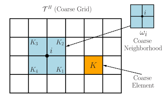
Figure 1: Illustration of a coarse neighborhood and a coarse element

Next, we briefly overview the continuous Galerkin (CG) formulation of GMsFEM, a generalization of the classical MsFEM [32]. For each coarse node $x_{i}$, we define a set of basis functions supported on the neighborhood $\omega_{i}$. We denote the $k$-th basis function supported on the coarse neighborhood $\omega_{i}$ by $\psi_{k}^{\omega_{i}}$, We remark that in the GMsFEM, we will use multiple basis functions per coarse neighborhood, and the index $k$ represents the local numbering of these basis functions. These multiscale basis functions are constructed from a local snapshot space and a local spectral decomposition defined on that snapshot space. The snapshot space contains a collection of many basis functions that can be used to capture most of the fine features of the solution, and the multiscale basis functions $\psi_{k}^{\omega_{i}}$ are constructed by selecting the dominant modes of a local spectral problem. Using the these multiscale basis functions, the CG solution is represented as $u_{\text{ms}}(x)=\sum_{i,k}c_{k}^{i}\psi_{k}^{\omega_{i}}(x)$. Once the basis functions are identified, the CG global coupling is given through the variational form

$$a(u_{\text{ms}},v)=(f,v),\quad\text{for all}\,\,v\in V_{\text{off}},$$ (4)

where $V_{\text{off}}$ is the space spanned by the basis functions $\{\psi_{k}^{\omega_{i}}\}$, and $a(\cdot,\cdot)$ is the usual bilinear form corresponding to (1). We remark that one can use other formulations, such as the discontinuous Galerkin formulation (see e.g., [12, 14, 20]), the mixed formulation (see e.g., [13, 8]) or the hybridized discontinuous Galerkin formulation (see e.g., [25]) to couple the multiscale basis functions.

In using GMsFEM, it is desirable to determine the number of basis functions per coarse neighhorbood adaptively based on the heterogeneities of the coefficient $\kappa(x)$ in order to obtain an efficient representation of the solution. In [16], a residual based a posteriori error indicator is derived and an adaptive basis enrichment algorithm is developed under the CG formulation. In particular, it is shown that

$$\|u-u_{\text{ms}}\|_{V}^{2}\leq C\sum_{i=1}^{N}r_{i}^{2},$$

where $r_{i}$ is the residual of the solution $u_{\text{ms}}$ on the coarse neighborhood $\omega_{i}$. Thus, local residuals of the multiscale solution give indicators to the error of the solution in the energy norm, and one can add basis functions to the coarse neighborhoods when the residuals $r_{i}$ are large. Convergence of this adaptive basis enrichment algorithm is also shown in [16]. On the other hand, for some applications one needs to adaptively construct new basis functions in the online stage in order to capture distant effects. In [15], such online adaptivity is proposed and mathematically analyzed. More precisely, when the local residual $r_{i}$ is large, one can construct a new basis function $\phi\in V_{0}(\omega_{i})$ in the online stage by solving

$$a(\phi,v)=(r_{i},v),\quad\forall v\in V_{0}(\omega_{i}),$$

where $V_{0}(\omega_{i})$ is the restriction of $V$ in $\omega_{i}$ with zero trace on $\partial\omega_{i}$. Numerical results in [15] show that a couple of these online basis functions can help to reduce the error by a large amount.

The adaptivity procedures discussed above are designed with the aim of reducing the error in the energy norm. In some applications, one may be more interested in reducing error measured by some function of the solution other than a norm. For example, in flow applications, one needs to obtain a good approximation of the pressure in locations where the wells are situated. Therefore, we now consider goal-oriented adaptivity within GMsFEM. Specifically, we define a linear functional $g:V\rightarrow\mathbb{R}$, referred to as the goal functional. In goal-oriented adaptivity, one wants to adaptively enrich the approximation space in order to reduce the goal error defined by $g(u-u_{\text{ms}})$. In the construction of goal-oriented adaptivity for GMsFEM, we use local indicators based on the solution of a dual problem: finding $z\in V$ such that

$$a^{*}(z,v)=g(v),\quad\forall v\in V.$$ (5)

For a primal problem $a(u,v)=(f,v)$ based on bilinear form $a(\,\cdot\,,\,\cdot\,)$, the dual form $a^{\ast}(\,\cdot\,,\,\cdot\,)$ is the formal adjoint of the primal, satisfying $a^{\ast}(w,v)=a(v,w)$, and in the current symmetric case, $a^{\ast}(\,\cdot\,,\,\cdot\,)$ is identical to the primal. Formally, the primal-dual equivalence follows for $u$ the solution to the primal problem (2) and $z$ the solution to the dual problem (5)

$$f(z)=a(u,z)=a^{\ast}(z,u)=a(z,u)=g(u).$$ (6)

Error estimates for the quantity of interest $g(u)$ follow from (6) and Galerkin orthogonality with respect to the discrete problems and their respective solutions. Forming error indicators based on both primal and dual problems and these estimates, we add multiscale basis functions to coarse neighborhoods when the values of the corresponding indicators are large. Our numerical examples show that the goal-oriented approach performs better than the residual approach for high-contrast problems when the error is measured by the goal-functional, $g(u-u_{\text{ms}})$.

3 The GMsFEM and residual-based adaptivity

In this section, we will give a detailed description of the GMsFEM (see for example [19, 21]) and it’s residual based adaptivity (see for example [16]).

3.1 Local basis functions

We first present the construction of the multiscale basis functions. This construction is performed in the offline stage; that is, basis functions are pre-computed before the actual solve of the problem. The construction starts with a snapshot space. This space contains a relatively large set of basis functions which can be used to capture most features of the fine-scale solution. The next step is to perform a local dimension reduction to obtain a lower dimensional subspace that can still be used to approximate the solution with good accuracy. The local dimension reduction is performed by solving a spectral problem, and the dominant eigenfunctions are used as the multiscale basis functions.

First, we define a snapshot space $V_{\text{snap}}^{\omega_{i}}$, where the functions in $V_{\text{snap}}^{\omega_{i}}$ are supported in $\omega_{i}$. The snapshot space can be the space of all fine-scale basis functions $V(\omega_{i})=\{v|_{\omega_{i}}\,|\,v\in V\}$ or the solutions of some local problems with various choices of boundary conditions. For example, we can use the following $\kappa$-harmonic extensions to form a snapshot space. Specifically, let $\{x_{j}^{i}\},~{}j=1,\ldots L_{i}$, index the set of fine-grid vertices that lie on the boundary of each coarse neighborhood, $\partial\omega_{i}$. Define the unit source functions $\delta_{j}^{h}(x)=\delta(x_{j}^{i})$ for each $j=1,\ldots L_{i}$. Then construct the snapshot function $\psi_{j}^{\omega_{i},\text{snap}}\in V(\omega_{i})$ by solving

$$\begin{split}-\text{div}(\kappa(x)\nabla\psi_{j}^{\omega_{i},\text{snap}})&=0,\quad\text{in}\,\,\,\omega_{i},\\ \psi_{j}^{\omega_{i},\text{snap}}&=\delta_{j}^{h},\quad\text{on}\,\,\,\partial\omega_{i}.\end{split}$$ (7)

The snapshot space $V_{\text{snap}}^{\omega_{i}}$ corresponding to the region $\omega_{i}$, then contains $L_{i}$ functions

$$V_{\text{snap}}^{\omega_{i}}=\text{span}\{\psi_{j}^{\omega_{i},\text{snap}}:~{}~{}~{}1\leq j\leq L_{i}\}.$$

We define the corresponding change of variable matrix

$$R_{\text{snap}}^{i}=\left[\psi_{1}^{\omega_{i},\text{snap}},\ldots,\psi_{L_{i}}^{\omega_{i},\text{snap}}\right],$$

where $\psi_{j}^{\omega_{i},\text{snap}}$ are considered as the columns of the matrix.

We next determine a set of dominant modes from $V_{\text{snap}}^{\omega_{i}}$, and the resulting lower dimensional space is called the offline space $V_{\text{off}}^{\omega_{i}}$. To construct the offline space $V_{\text{off}}^{\omega_{i}}$, we perform a dimension reduction of the space of snapshots using an auxiliary spectral decomposition. The analysis in [23] motivates the following generalized eigenvalue problem for eigenvalues $\lambda_{k}^{\text{off}}$ and eigenfunctions $\Psi_{k}^{\text{off}}$ in the space of snapshots:

$$A^{\text{off}}\Psi_{k}^{\text{off}}=\lambda_{k}^{\text{off}}S^{\text{off}}\Psi_{k}^{\text{off}},$$ (8)

where

$$A^{\text{off}}=[a_{mn}^{\text{off}}]=\int_{\omega}\kappa(x)\nabla\psi_{m}^{\text{snap}}\cdot\nabla\psi_{n}^{\text{snap}}=(R^{i}_{\text{snap}})^{T}AR^{i}_{\text{snap}},$$

and

$$S^{\text{off}}=[s_{mn}^{\text{off}}]=\int_{\omega}\widetilde{\kappa}(x)\psi_{m}^{\text{snap}}\psi_{n}^{\text{snap}}=(R^{i}_{\text{snap}})^{T}SR^{i}_{\text{snap}},$$

where $A$ and $S$ denote analogous fine-scale stiffness and mass matrices as defined by

$$A_{ij}=\int_{D}\kappa(x)\nabla\phi_{i}\cdot\nabla\phi_{j}\,dx,\quad S_{ij}=\int_{D}\widetilde{\kappa}(x)\phi_{i}\phi_{j}\,dx,$$

where $\phi_{i}$ is the fine-scale basis function for $V$. We will give the definition of $\widetilde{\kappa}(x)$ later on. To generate the offline space we then select the smallest $l_{i}$ eigenvalues from Equation (8) and form the corresponding eigenvectors in the space of snapshots by setting $\psi_{k}^{\omega_{i},\text{off}}=\sum_{j=1}^{L_{i}}\Psi_{kj}^{\text{off}}\psi_{j}^{\omega_{i},\text{snap}}$ (for $k=1,\ldots,l_{i}$), where $\Psi_{kj}^{\text{off}}$ are the coordinates of the vector $\Psi_{k}^{\text{off}}$, and $l_{i}$ is the number of eigenvectors chosen to span the offline space. We will use the set $\{\psi_{k}^{\omega_{i},\text{off}}\}$ of local basis functions to form the approximation space in the next section.

3.2 CG formulation

In this section we create an appropriate solution space and the variational formulation for a continuous Galerkin approximation of Equation (1). The idea is to use the basis set $\{\psi_{k}^{\omega_{i},\text{off}}\}_{k=1}^{l_{i}}$, $i=1,2,\cdots,N$, to form the approximation space, called the offline space, and apply the standard continuous Galerkin formulation. We begin with an initial coarse space $V^{\text{init}}_{0}=\text{span}\{\chi_{i}\}_{i=1}^{N}$, where we recall $N$ denotes the number of coarse neighborhoods corresponding to interior coarse nodes. Here, $\chi_{i}$ are the standard multiscale partition of unity functions which are supported in $\omega_{i}$ and are defined by

$$-\text{div}\left(\kappa(x)\,\nabla\chi_{i}\right) =0,\quad\text{in}\,\,\,K\subset\omega_{i},$$ (9)

$$\chi_{i} =g_{i},\quad\text{on}\,\,\,\partial K\backslash\partial\omega_{i},$$

$$\chi_{i} =0,\quad\text{on}\,\,\,\partial\omega_{i},$$

for all coarse elements $K\subset\omega_{i}$, where $g_{i}$ is a continuous function on $\partial K$ which is linear on each edge of $\partial K$. Based on the analysis in [23], the summed, pointwise energy $\widetilde{\kappa}$ required for the eigenvalue problems (8) is defined as

$$\widetilde{\kappa}=\kappa\sum_{i=1}^{N}H^{2}|\nabla\chi_{i}|^{2},$$

where $H$ denotes the coarse mesh size.

The partition of unity functions $\chi_{i}$ are then multiplied by the eigenfunctions $\{\psi_{k}^{\omega_{i},\text{off}}\}_{k=1}^{l_{i}}$ to construct the multiscale basis functions

$$\psi_{i,k}=\chi_{i}\psi_{k}^{\omega_{i},\text{off}},\quad\text{for}\,\,\,1\leq i\leq N\,\,\,\text{and}\,\,\,1\leq k\leq l_{i},$$ (10)

where we recall $l_{i}$ denotes the number of offline eigenvectors that are chosen for each coarse node $i$. We note the construction in Equation (10) yields continuous basis functions due to the multiplication of offline eigenvectors with the initial (continuous) partition of unity. Next, we define the continuous Galerkin spectral multiscale space as

$$V_{\text{off}}=\text{span}\{\psi_{i,k}:\,\,1\leq i\leq N\,\,\,\text{and}\,\,\,1\leq k\leq l_{i}\}.$$ (11)

Using this offline space, we obtain the GMsFEM as in (4).

3.3 Residual-based adaptivity

In this section, we give a brief review of the adaptive basis enrichment algorithm proposed in [16]. After solving the coarse mesh problem and computing error indicators, the standard Dörfler marking strategy is applied with respect to the neighborhoods indexed by vertices $i=1,\ldots,N$, rather than the elements $K$. The marked neighborhoods are then enriched with additional basis functions. The spectral problem (8) gives a natural ordering of basis functions in the local snapshot space $V^{\omega_{i}}_{\text{snap}}$ with respect to the eigenvalues, in increasing order. The analysis of [16] then suggests an adaptive procedure to add basis functions based on a local error indicator. The error indicator is defined by a $H^{-1}$-norm based residual, which gives a robust indicator with good performance for cases with high contrast media.

Let $\omega_{i}$ be a coarse neighborhood and write $V_{i}=V_{0}(\omega_{i})$. For a given multiscale solution $u_{\text{ms}}$, we define a linear functional $R^{u}_{i}(v)$ on $V_{i}$ by

$$R^{u}_{i}(v)=\int_{\omega_{i}}fv-\int_{\omega_{i}}\kappa\nabla u_{\text{ms}}\cdot\nabla v,\quad v\in V_{i}.$$ (12)

The norm of $R^{u}_{i}$ is defined as

$$\|R^{u}_{i}\|_{V_{i}^{*}}=\sup_{v\in V_{i}}\frac{|R^{u}_{i}(v)|}{\|v\|_{V_{i}}}.$$ (13)

where $\|v\|_{V_{i}}^{2}=\int_{\omega_{i}}\kappa(x)|\nabla v|^{2}\,dx$. The norm $\|R^{u}_{i}\|_{V_{i}^{*}}$ gives a measure on how well the solution $u_{\text{ms}}$ satisfies the variational problem (2) restricted to $V_{i}$. The norm $\|R^{u}_{i}\|_{V_{i}^{*}}$ can be obtained by solving an auxiliary problem of finding $w\in V_{i}$ such that $a(w,v)=R_{i}^{u}(v)$ for all $v\in V_{i}$ and then setting $\|R^{u}_{i}\|_{V_{i}^{*}}=\|w\|_{V}$. One can solve this auxiliary problem in the snapshot space $V_{\text{snap}}^{\omega_{i}}$ to reduce the computational cost. Moreover, in [16] the following a posteriori error bound is proved

$$\|u-u_{\text{ms}}\|_{V}^{2}\leq C_{\text{\rm err}}\sum_{i=1}^{N}\|R^{u}_{i}\|^{2}_{V_{i}^{*}}(\lambda^{\omega_{i}}_{l_{i}+1})^{-1},$$ (14)

where $C_{\text{err}}$ is a uniform constant independent of the contrast of $\kappa$, and $\lambda_{j}^{\omega_{i}}$ is the $j$-th eigenvalue of the eigenvalue problem (8) for the coarse neighborhood $\omega_{i}$. In particular, $\lambda_{l_{i}+1}^{\omega_{i}}$ is the first, i.e., smallest eigenvalue from the spectral problem (8) for which the corresponding eigenvector is not included in the construction of the offline space.

Using the above error bound (14), a convergent adaptive enrichment algorithm is developed in [16]. We now describe this algorithm. The algorithm is an iterative process, and basis functions are added in each iteration/level based on the magnitudes of local residuals. We use $m\geq 1$ to index the enrichment level and let $V_{\text{off}}^{m}$ be the solution space at the $m$-th iteration. For each coarse region, let $l_{i}^{m}$ be the number of eigenfunctions used at the enrichment level $m$ for the coarse region $\omega_{i}$.

3.4 Adaptive algorithm

The adaptive enrichment algorithm for GMsFEM is now summarized below. Choose a fixed marking parameter $0<\theta<1$. Choose also an initial offline space $V_{\text{off}}^{1}$ by specifying a fixed number of basis functions for each coarse neighborhood, and this number is denoted by $l_{i}^{1}$, for each $i=1,\ldots,N$. Then, generate a sequence of spaces $V_{\text{off}}^{m}$ and a sequence of multiscale solutions $u_{\text{ms}}^{m}$ obtained by solving (4). Specifically, for each $m=1,2,\cdots$, perform the following calculations:

1. Find the multiscale solution in the current space. That is, find $u_{\text{ms}}^{m}\in V^{m}_{\text{off}}$ such that

   $$a(u^{m}_{\text{ms}},v)=(f,v)\quad\text{for all}\,\,\,v\in V^{m}_{\text{off}}.$$ (15)

2. Compute the local residual. For each coarse region $\omega_{i}$, compute

   $$\eta^{2}_{i}=\|R_{i}^{u}\|^{2}_{V_{i}^{*}}(\lambda^{\omega_{i}}_{l^{m}_{i}+1})^{-1},$$

   where

   $$R_{i}^{u}(v)=\int_{\omega_{i}}fv-\int_{\omega_{i}}\kappa(x)\nabla u^{m}_{\text{ms}}\cdot\nabla v,$$

   consistent with (12), and the norm is defined in (13) respectively. Next, re-enumerate the coarse neighborhoods so the above local residuals $\eta_{i}^{2}$ are arranged in decreasing order $\eta^{2}_{1}\geq\eta^{2}_{2}\geq\cdots\geq\eta^{2}_{N}$. That is, in the new enumeration, the coarse neighborhood $\omega_{1}$ has the largest residual $\eta_{1}^{2}$ and the coarse neighborhood $\omega_{N}$ has the least residual $\eta_{N}^{2}$.

   Remark 3.1.

   An alternate approach to avoid the $N\log N$ complexity of the full sort is the standard binning or heapifying strategy [36]. Let $\eta^{2}=\sum_{i=1}^{n}\eta_{i}^{2}$, and consider only $\eta_{i}$ that satisfy $\eta_{i}^{2}>(1-\theta)\eta^{2}/N$. Let $M=\max_{i}\eta_{i}^{2}$, and perform a partial sort of the remaining indicators collecting or binning the indices for which $2^{-p}M\leq\eta_{i}^{2}<2^{-(p+1)}M$, for $p=0,2,\ldots q$, where $q$ is the smallest integer to satisfy $2^{-(q+1)}M\leq(1-\theta)\eta^{2}/N.$

3. Find the coarse regions where enrichment is needed. Choose the smallest integer $k$ such that

   $$\theta\sum_{i=1}^{N}\eta_{i}^{2}\leq\sum_{i=1}^{k}\eta_{i}^{2}.$$ (16)

   The coarse neighborhoods $\omega_{1},\omega_{2},\cdots,\omega_{k},$ are then enriched with additional basis functions. If the partial sort of Remark 3.1 is used in place of the sort, elements are marked by emptying the first bin, those indicators with $M\leq\eta_{i}^{2}<M/2$, and then continuing on to the second bin, and so forth until (16) is satisfied. As elements within bins are not sorted, this yields a quasi-optimal marked set, i.e., the marked set may not be the set of least-cardinality to satisfy (16) as in the full sort, but it is within a factor of two of the least cardinality.

4. Enrich the space. For each $i=1,2,\cdots,k$, add basis function for the region $\omega_{i}$ according to the following rule. Let $s$ be the positive integer such that $\lambda_{l_{i}^{m}+s+1}$ is large enough compared with $\lambda_{l_{i}^{m}+1}$ (see Remark 3.2). Then include the eigenfunctions $\Psi^{\text{off}}_{l_{i}^{m}+1},\cdots,\Psi^{\text{off}}_{l_{i}^{m}+s}$ in the construction of the basis functions. The resulting space is denoted as $V_{\text{off}}^{m+1}$. Mathematically, the space $V_{\text{off}}^{m+1}$ is defined as

   $$V_{\text{off}}^{m+1}=V_{\text{off}}^{m}+\text{span}\cup_{i=1}^{k}\cup_{j=l_{i}^{m}+1}^{l_{i}^{m}+s}\{\psi_{i,j}\}$$

   where $\psi_{i,j}=\chi_{i}\psi_{j}^{\omega_{i},\text{off}}$ and $\psi_{j}^{\omega_{i},\text{off}}=\sum_{r=1}^{l_{i}}\Psi_{jr}^{\text{off}}\psi_{r}^{\text{snap}}$, with $j=l_{i}^{m}+1,\cdots,l_{i}^{m}+s$, denote the new basis functions obtained by the eigenfunctions $\Psi^{\text{off}}_{l_{i}^{m}+1},\cdots,\Psi^{\text{off}}_{l_{i}^{m}+s}$. In addition, we set $l_{i}^{m+1}=l_{i}^{m}+s$.

   Remark 3.2.

   The mathematical analysis in [16] specifies the choice of $s$. In practice, one can take $s=1$ since the eigenvalues in (8) have fast growth.

4 Goal-oriented adaptivity

In this section, we present a goal-oriented adaptive enrichment algorithm for GMsFEM. The goal-oriented variant of the adaptive method requires the solution of a dual problem in addition to the primal at each iteration. The indicators are computed with both the primal residual and either the dual residual or a projection of an enriched dual solution into the primal space. These indicators predict which neighborhoods to enrich to increase the quality of the approximation of the quantity of interest. After introduction of the discrete dual problem, the finite dimensional analogue of (5), we propose two error indicators for goal-oriented enrichment.

The dual problem plays a vital role in goal-oriented adaptivity as the vehicle for introducing the goal functional $g$ into the adaptive process. Given a goal functional $g:V\rightarrow\mathbb{R}$, we define the discrete dual problem on approximation space $V_{\text{off}}\subset V$ as: find $z\in V_{\text{off}}$ such that

$$a(v,z)=g(v),\;\forall v\in V_{\text{off}}.$$ (17)

As in (5), the discrete dual form $a^{\ast}(\,\cdot\,,\,\cdot\,)$ is identical to the primal $a(\,\cdot\,,\,\cdot\,)$ for symmetric problems. The dual problem, however, features the goal functional $g$ as the source. The discrete dual solution, may now be used to define goal-oriented error indicators.

$H^{-1}$-based goal-oriented indicator

Our first goal-oriented indicator is similar in form to the residual based indicator described in the previous section. To motivate this indicator, we introduce the local bilinear form $a(u,v)_{i}=\int_{\omega_{i}}\kappa(x)\nabla u\cdot\nabla v\,dx$, and the induced localized energy norm $\left\|v\right\|_{V,i}=a(v,v)_{i}$. Let $u$ be the solution to (2), $u_{ms}\in V_{\text{off}}$ be the solution to (4), $z$ the solution to (5), and $z_{ms}\in V_{\text{off}}$ the solution to (17). Using Galerkin orthogonality and the relation between the primal and dual problems, the error in the quantity of interest satisfies

$$g(u-u_{ms}) =a(z,u-u_{ms})=a(u-u_{ms},z)=a(u-u_{ms},z-z_{ms}).$$ (18)

Decomposing the global integration into neighborhoods by the partition of unity functions $\chi_{i}$ given by (9)

$$a(u-u_{ms},z-z_{ms}) =\sum_{i=1}^{n}\int_{\Omega}\chi_{i}\kappa\nabla(u-u_{ms})\cdot\nabla(z-z_{ms})\;dx\leq\sum_{i=1}^{n}\left\|u-u_{ms}\right\|_{V,i}\left\|z-z_{ms}\right\|_{V,i}$$ (19)

where we used the fact that $\chi_{i}$ is supported in $\omega_{i}$ and the fact that $|\chi_{i}|\leq 1$. Instead of using the norm of local residual for the primal problem defined in (13) to be our indicator, (19) suggests using the product of norms of local residuals for the primal and dual problems, posed in the same discrete space, $V_{\text{off}}$. The local dual residual $R^{z}_{i}:V_{i}\rightarrow\mathbb{R}$ is defined by

$$R^{z}_{i}(v)=g(v)-\int_{\omega_{i}}\kappa(x)\nabla z_{\text{ms}}\cdot\nabla v,$$ (20)

where $z_{\text{ms}}\in V_{\text{off}}$ is the solution to (17). Analogous to (13), the $H^{-1}$ norm of $R^{z}_{i}$ is defined as

$$\|R^{z}_{i}\|_{V_{i}^{*}}=\sup_{v\in V_{i}}\frac{|R^{z}_{i}(v)|}{\|v\|_{V_{i}}}.$$ (21)

The local version of  (14), applied to both primal and dual residuals, namely

$$\left\|u-u_{ms}\right\|_{V,i}\leq C\left\|R_{i}^{u}\right\|_{V_{i}^{\ast}}(\lambda_{l_{i}+1}^{\omega_{i}})^{-1/2},\quad\left\|z-z_{ms}\right\|_{V,i}\leq C\left\|R_{i}^{z}\right\|_{V_{i}^{\ast}}(\lambda_{l_{i}+1}^{\omega_{i}})^{-1/2},$$ (22)

motivates the local error indicator, $\eta_{i}$, defined as

$$\eta^{2}_{i}=\|R^{z}_{i}\|_{V_{i}^{*}}\|R^{u}_{i}\|_{V_{i}^{*}}(\lambda^{\omega_{i}}_{l_{i}+1})^{-1},$$ (23)

where $\|R^{u}_{i}\|_{V_{i}^{*}}$ and $\|R^{z}_{i}\|_{V_{i}^{*}}$ are defined in (13) and (21), respectively. Applying (23) and (22) to (19) bounds the error in the goal function by

$$g(u-u_{ms})\leq C\sum_{i=1}^{n}\eta_{i}^{2}.$$ (24)

In summary, the goal-error over the global domain $D$ is bounded by the product of energy errors of the primal and dual problems, which is in turn bounded by the sum of the indicators given by (23), modified by the partition of unity functions. This upper bounds suggests the adequacy of the indicators in reducing the error. The efficiency and a formal convergence analysis are however not addressed here. As in [6] where a similar indicator is used for $hp$-refinement, this indicator displays similar behavior to the DWR-type indicator, as shown in the numerical experiments; however, it is more amenable to analysis. This indicator has the added advantage of reduced computational cost as compared to the DWR-type indicator described below, as both primal and dual problems are solved over the same discrete spaces, whereas for the DWR-type method, the dual problem has greater computational complexity than the primal.

DWR-type goal-oriented indicator

The next error indicator is similar to DWR error indicator. For the primal problem solved in discrete space $V_{\text{off}}$, the DWR indicator is motived by the following residual equation. For $z$ the solution to (5), $u$ the solution to (2), and $u_{ms}\in V_{\text{off}}$ the solution to (4)

$$g(u-u_{ms})=a(u-u_{ms},z-z_{\text{off}})=R^{u}(z-z_{\text{off}}),$$ (25)

where $z_{\text{off}}$ in $V_{\text{off}}$ is arbitrary and the global residual $R^{u}(v)=\int_{D}fv-\int_{D}\kappa(x)\nabla u_{\text{ms}}\cdot\nabla v$. We let $z_{\text{off}}^{i}$ be the component of $z_{\text{off}}$ spanned by the basis functions corresponding to the coarse neighborhood $\omega_{i}$. Localizing (25) by the partition of unity functions $\chi_{i}$,

$$R^{u}(z-z_{\text{off}})=\sum_{i=1}^{N}R_{i}^{u}\Big{(}\chi_{i}z-z_{\text{off}}^{i}\Big{)}=\sum_{i=1}^{N}R_{i}^{u}\Big{(}z_{\text{enrich}}^{i}-z_{\text{off}}^{i}\Big{)}+\sum_{i=1}^{N}R_{i}^{u}\Big{(}\chi_{i}z-z_{\text{enrich}}^{i}\Big{)}.$$ (26)

As the exact solution $z$ is unavailable, one generally instead replaces $z$ by $z_{\text{enrich}}$, a discrete solution from a more enriched space than the primal, essentially neglecting the last term of (26). The function $z_{\text{enrich}}^{i}$ is the component of $z_{\text{enrich}}$ spanned by the basis functions corresponding to the coarse neighborhood $\omega_{i}$. In standard finite element methods the global residual is then solved elementwise and used as an indicator. By Galerkin orthogonality, then function $z_{\text{off}}$ may be taken as any function in $V_{\text{off}}$ but in practice is taken as the projection of the enriched dual solution into $V_{\text{off}}$.

In this case, the dual problem is solved in the enriched space, called $V_{\text{enrich}}$. The space $V_{\text{enrich}}$ is obtained by adding more basis functions to each coarse neighborhood. Recalling the construction of basis functions $\psi_{i,k}$ in (10), the enriched space is constructed with more than $l_{i}$ basis functions per coarse neighborhood, specifically

$$\psi_{i,k}=\chi_{i}\psi_{k}^{\omega_{i},\text{off}},\quad\text{for}\,\,\,1\leq i\leq N\,\,\,\text{and}\,\,\,1\leq k\leq l_{i}+m,$$ (27)

where $m$ basis functions are added for each $\omega_{i}$. The span of these basis is our $V_{\text{enrich}}$. Let $z_{\text{enrich}}\in V_{\text{enrich}}$ be the solution for the dual problem in $V_{\text{enrich}}$, that is, $z_{\text{enrich}}$ satisfies

$$a(v,z_{\text{enrich}})=g(v),\;\forall v\in V_{\text{enrich}}.$$ (28)

The DWR-type error estimator is defined as

$$\eta^{2}_{i}=\Big{|}R^{u}_{i}\Big{(}P_{i}(z_{\text{enrich}})-\pi\big{(}P_{i}(z_{\text{enrich}})\big{)}\Big{)}\Big{|},\quad\quad i=1,2,\cdots,N.$$ (29)

In the above definition, $P_{i}(z_{\text{enrich}})$ is the component of $z_{\text{enrich}}$ spanned by the basis functions $\psi_{i,k}$, $k=1,2,\cdots,l_{i}+m$, corresponding to the coarse neighborhood $\omega_{i}$. Moreover $\pi\big{(}P_{i}(z_{\text{enrich}})\big{)}$ is the component of $P_{i}(z_{\text{enrich}})$ spanned by the basis functions $\psi_{i,k}$, $k=1,2,\cdots,l_{i}$, in the offline space. Comparison with (26) yields an heuristic bound, modulo the error term created by replacing $z$ by $z_{\text{enrich}}$.

Each of the two indicators, given by (23), and respectively, (29), may be implemented in an adaptive framework to determine which coarse neighborhoods to enrich. The goal-oriented variant of the adaptive enrichment algorithm in Section 3.4 is now described.

Goal-oriented adaptive enrichment algorithm

Choose a fixed marking parameter $0<\theta<1$. Choose also an initial offline space $V_{\text{off}}^{1}$ by specifying a fixed number of basis functions for each coarse neighborhood, and this number is denoted by $l_{i}^{1}$. Then, generate a sequence of spaces $V_{\text{off}}^{m}$ and a sequence of multiscale solutions $u_{\text{ms}}^{m}$ obtained by solving (4). Specifically, for each $m=1,2,\cdots$, perform the following calculations:

1. Find the multiscale solution in the current space. That is, find $u_{\text{ms}}^{m}\in V^{m}_{\text{off}}$ such that

   $$a(u^{m}_{\text{ms}},v)=(f,v)\quad\text{for all}\,\,\,v\in V^{m}_{\text{off}}.$$ (30)

2. Find the multiscale dual solution in the current space or an enriched space. That is, find $z_{\text{ms}}^{m}\in V^{m}_{\text{dual}}$ such that

   $$a(z^{m}_{\text{ms}},v)=(f,v)\quad\text{for all}\,\,\,v\in V^{m}_{\text{dual}}$$ (31)

   where

   $$V^{m}_{\text{dual}}=\begin{cases}V^{m}_{\text{off}},&\text{ for $H^{-1}$-based error estimator},\\ V^{m}_{\text{enrich}},&\text{ for DWR-type error estimator}.\end{cases}$$

3. Compute the local residual. For each coarse region $\omega_{i}$, compute

   $$\eta^{2}_{i}=\begin{cases}\|R^{z}_{i}\|_{V_{i}^{*}},\|R^{u}_{i}\|_{V_{i}^{*}}(\lambda^{\omega_{i}}_{l_{i}+1})^{-1},&\text{ for $H^{-1}$-based error estimator},\\ \big{|}R^{u}_{i}(P_{i}(z_{\text{enrich}})-\pi(P_{i}(z_{\text{enrich}})))\big{|},&\text{ for DWR-type error estimator}.\end{cases}$$

   $$R^{u}_{i}(v) =\int_{\omega_{i}}fv-\int_{\omega_{i}}\kappa(x)\nabla u^{m}_{\text{ms}}\cdot\nabla v,$$

   $$R^{z}_{i}(v) =\int_{\omega_{i}}gv-\int_{\omega_{i}}\kappa(x)\nabla z^{m}_{\text{ms}}\cdot\nabla v,$$

   consistent with (12) and (20); and the norm is defined in (13) and (21) respectively. Next, re-enumerate the coarse neighborhoods so that the above local residuals $\eta_{i}^{2}$ are arranged in decreasing order $\eta^{2}_{1}\geq\eta^{2}_{2}\geq\cdots\geq\eta^{2}_{N}$. That is, in the new enumeration, the coarse neighborhood $\omega_{1}$ has the largest residual $\eta_{1}^{2}$. As in Remark 3.1 the full sort of the estimators can be replaced by a partial sort for a marked set of quasi-optimal cardinality.

4. Find the coarse regions where enrichment is needed. Choose the smallest integer $k$ such that

   $$\theta\sum_{i=1}^{N}\eta_{i}^{2}\leq\sum_{i=1}^{k}\eta_{i}^{2}.$$ (32)

   The coarse neighborhoods $\omega_{1},\omega_{2},\cdots,\omega_{k},$ are then enriched with additional basis functions. Alternately, a set of neighborhoods based on the binning strategy for a partial sort can be chosen as described in Step 3 of the Adaptive algorithm 3.4.

5. Enrich the space. For each $i=1,2,\cdots,k$, add basis functions for the region $\omega_{i}$ according to the following rule. Let $s$ be the smallest positive integer such that $\lambda_{l_{i}^{m}+s+1}$ is large enough compared with $\lambda_{l_{i}^{m}+1}$. Then include the eigenfunctions $\Psi^{\text{off}}_{l_{i}^{m}+1},\cdots,\Psi^{\text{off}}_{l_{i}^{m}+s}$ in the construction of the basis functions. The resulting space is denoted as $V_{\text{off}}^{m+1}$. Mathematically, the space $V_{\text{off}}^{m+1}$ is defined as

   $$V_{\text{off}}^{m+1}=V_{\text{off}}^{m}+\text{span}\cup_{i=1}^{k}\cup_{j=l_{i}^{m}+1}^{l_{i}^{m}+s}\{\psi_{i,j}\}$$

   where $\psi_{i,j}=\chi_{i}\psi_{j}^{\omega_{i},\text{off}}$ and $\psi_{j}^{\omega_{i},\text{off}}=\sum_{r=1}^{l_{i}}\Psi_{jr}^{\text{off}}\psi_{r}^{\text{snap}}$, with $j=l_{i}^{m}+1,\cdots,l_{i}^{m}+s$, denote the new basis functions obtained by the eigenfunctions $\Psi^{\text{off}}_{l_{i}^{m}+1},\cdots,\Psi^{\text{off}}_{l_{i}^{m}+s}$. In addition, set $l_{i}^{m+1}=l_{i}^{m}+s$.

In the next section, we demonstrate the efficiency of the goal-oriented adaptive algorithm defined above on a problem with high-contrast multiscale coefficients. The results are compared with the standard residual-based adaptive method defined in the previous section. We note both the increased efficiency in the reduction in goal-error, $|g(u-u_{ms})|$, and the decreased reduction in the energy-norm error with the goal-oriented methods. These two observations suggest the method does what it was designed to do: focus the adaptive enrichment towards reduction in goal-error without resolving the solution where it has limited influence on the goal-error. We also note similarity in performance between the two indicators, both demonstrating errors with a similar observed rate of convergence.

5 Numerical Results

In this section, we present two numerical examples for multiscale problems with high-contrast coefficients and compare the performance of the two indicators defined in the previous section. For our simulations, we take the domain $\Omega=(0,1)^{2}$, and the inflow-outflow source term $f=\chi_{K_{1}}-\chi_{K_{2}}$, where $K_{1}=[0.1,0.2]\times[0.8,0.9]$, and $K_{2}=[0.8,0.9]\times[0.1,0.2]$. We consider the problem of finding $g(u)$ for $u$ the solution to (1), namely

$$-\text{div}(\kappa(x)\nabla u)=f,~{}\text{ in }~{}D,\quad u=0~{}\text{ on }~{}\partial D.$$ (33)

The goal functional

$$g(u)=\int_{K_{2}}u,$$

is the average value of $u$ on the outflow region $K_{2}$. In practice, $K_{2}$ is the location of the wells, and it is important that the average pressure $u$ on $K_{2}$ is accurate. The two examples differ by the high-contrast coefficients $\kappa(x)$, shown in Figure 2. Shown on the left, $\kappa_{1}$ features a high-conductivity channel crossing the domain separating the inflow and outflow; on the right, $\kappa_{2}$ is a similar coefficient without the channel. These coefficents are visualized with the blue region indicating the value $1$ and the red region indicating the contrasts. In each example, we consider two different contrast strengths, $10^{4}$ and $10^{6}$. We note the invariance in the relative performance of the indicators with respect to the contrast strengths.

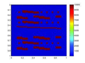
Figure 2: Left: the coefficient $\kappa_{1}$, corresponding to Figure 3. Right: the coefficient $\kappa_{2}$, corresponding to Figure 4.

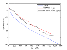
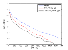
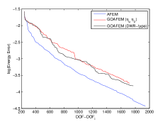
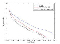
Figure 3: Lower contrast ($10^{4}$). Top left: $\log\|u-u_{ms}\|_{V}$. Top right: $\log|g(u-u_{ms})|$.
Higher contrast ($10^{6}$). Bottom left: $\log\|u-u_{ms}\|_{V}$, Bottom right: $\log|g(u-u_{ms})|$.

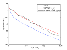
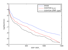
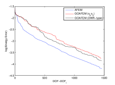
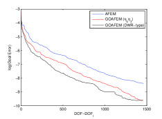
Figure 4: Lower contrast ($10^{4}$). Top left: $\log\|u-u_{ms}\|_{V}$, Top right: $\log|g(u-u_{ms})|$.
Higher contrast($10^{6}$), Bottom left: $\log\|u-u_{ms}\|_{V}$, Bottom right: $\log|g(u-u_{ms})|$.

For the first example, Figure 3 shows a comparison in error reduction between the three indicators for coefficient $\kappa_{1}$. In the two figures on the right, we compare the logarithms of the energy norm errors $g(u-u_{\text{ms}})$ against the number of unknowns for three types of adaptive enrichment algorithms; namely, the residual based method described in Section 3.4 (denoted in blue in Figure 3), the $H^{-1}$ residual-based goal-oriented method (denoted in red in Figure 3), and the DWR type goal-oriented method (denoted in black in Figure 3) as described in Section 4. From these results, we see the two types of goal-oriented methods behave similarly and outperform the standard adaptive method with an improved rate of goal-error reduction. We note a more stable decrease in error reduction for the goal-oriented residual-type method, but slightly improved, if less predictable error reduction for the DWR-type. This last observation is to be expected, as the DWR-type indicator does not account for the error created by using the enriched solution $z_{\text{enrich}}$ in place of the exact dual solution $z$, as in (26).

On the left of Figure 3, we see the standard residual based method outperforms the goal-oriented methods for the energy norm error, $\|u-u_{\text{ms}}\|_{V}$. This confirms that the goal-oriented methods are driving the adaptivity toward a more efficient evaluation of the quantity of interest without expending additional computational effort resolving features of the solution with limited influence on the goal.

For the second example, we consider finding $g(u)$ for $u$ that satisfies  (33), with $\kappa(x)$ given by $\kappa_{2}$ shown on the right of Figure 2, with no high-conductivity channel. As seen in Figure 4, the results are qualitatively similar to the results of the first example. In summary, the plots on the right show the goal-error reduction for the higher and respectively lower contrast cases. The residual-type and DWR-type goal-oriented indicators achieve a better rate of error reduction than the standard adaptive method, with the DWR-type showing generally the lowest error, with the least-steady decrease. The plots on the right of Figure  4 show the reduction of energy error for the three indicators. As in the first example, the standard $H^{-1}$ residual based adaptive method designed to reduce the energy error shows the best performance here, whereas the goal-oriented methods yield steady error reduction but are focused on localized error reduction in the region of the goal-functional, rather than across the entire domain.

These results demonstrate the importance of goal-oriented adaptivity in GMsFEM, particularly in cases where the global domain is significantly larger than the region of infuence for the quantity of interest. In partiuclar, problems with many localized features only some of which significantly influence the quantity of interest will benefit from a goal-oriented adaptive strategy.

6 Conclusion

In this paper we defined two types of error indicators that can be used in an adaptive algorithm for multiscale problems with high-contrast coefficients. The goal-oriented adaptive algorithm fits within the framework of GMsFEM, and focuses the adaptivity on reducing the error in the quantity of interest, rather than in global norm. We first reviewed the general ideas of GMsFEM for high-contrast problems, then gave a detailed overview of the construction of multiscale basis functions, and a residual based adaptive algorithm designed to reduce the energy norm error. We stated the dual problem, then motivated and introduced two goal-oriented error indicators, and described their use in a a goal-oriented adaptive algorithm. Finally, we demonstrated the efficiency of the goal-oriented algorithm and estimators compared with the standard adaptive method introduced earlier. We found for both indicators, the goal-oriented method reduced the error in the goal-function at a better rate than the standard method. We also found the two indicators perform similarly, with some increase in error reduction seen in the DWR-type indicator, but at the cost of solving the dual problem in a more enriched space, increasing the computational complexity. The residual-based indicator on the other hand may be more amenable to convergence analysis, as may be investigated in future work. The current results indicate the goal-oriented strategy increases the efficiency of GMsFEM when a function of the solution rather than the solution in its entirety is of interest.

References

- [1] J.E. Aarnes, S. Krogstad, and K.-A. Lie. A hierarchical multiscale method for two-phase flow based upon mixed finite elements and nonuniform grids. SIAM J. Multiscale Modeling and Simulation, 5(2):337–363, 2006.
- [2] T. Arbogast, G. Pencheva, M.F. Wheeler, and I. Yotov. A multiscale mortar mixed finite element method. Multiscale Model. Simul., 6(1):319–346 (electronic), 2007.
- [3] W. Bangerth and R. Rannacher. Adaptive finite element methods for differential equations. Birkhauser, Boston, 2003.
- [4] R. Becker and R. Rannacher. An optimal control approach to a posteriori error estimation in finite element methods. Acta Numerica, 10:1–102, 2001.
- [5] P. Binev, W. Dahmen, and R. DeVore. Adaptive finite element methods with convergence rates. Numer. Math., 97(2):219–268, 2004.
- [6] M. Buerg and M. Nazarov. Goal-oriented adaptive finite element methods for elliptic problems revisited. J. Comput. Appl. Math., 287:125 – 147, 2015.
- [7] J. M. Cascon, C. Kreuzer, R. H. Nochetto, and K. G. Siebert. Quasi-optimal convergence rate for an adaptive finite element method. SIAM J. Numer. Anal., 46(5):2524–2550, 2008.
- [8] H. Y. Chan, E. Chung, and Y. Efendiev. Adaptive mixed gmsfem for flows in heterogeneous media. arXiv preprint arXiv:1507.01659, 2015.
- [9] Y. Chen and L. Durlofsky. An ensemble level upscaling approach for efficient estimation of fine-scale production statistics using coarse-scale simulations. In SPE Reservoir Simulation Symposium, Houston, Texas, U.S.A., 2 2007. Society of Petroleum Engineers.
- [10] Y. Chen, L. Durlofsky, M. Gerritsen, and X. Wen. A coupled local-global upscaling approach for simulating flow in highly heterogeneous formations. Advances in Water Resources, 26:1041–1060, 2003.
- [11] E. Chung and Y. Efendiev. Reduced-contrast approximations for high-contrast multiscale flow problems. SIAM J. Multiscale Modeling and Simulation, 8:1128–1153, 2010.
- [12] E. Chung, Y. Efendiev, and R. Gibson. An energy-conserving discontinuous multiscale finite element method for the wave equation in heterogeneous media. Advances in Adaptive Data Analysis, 3:251–268, 2011.
- [13] E. Chung, Y. Efendiev, and C. S. Lee. Mixed generalized multiscale finite element methods and applications. Multiscale Modeling & Simulation, 13(1):338–366, 2015.
- [14] E. Chung, Y. Efendiev, and W. T. Leung. Generalized multiscale finite element methods for wave propagation in heterogeneous media. Multiscale Modeling & Simulation, 12(4):1691–1721, 2014.
- [15] E. Chung, Y. Efendiev, and W. T. Leung. Residual-driven online generalized multiscale finite element methods. arXiv preprint arXiv:1501.04565, 2015.
- [16] E. Chung, Y. Efendiev, and G. Li. An adaptive gmsfem for high-contrast flow problems. Journal of Computational Physics, 273:54–76, 2014.
- [17] E. Chung, Y. Efendiev, G. Li, and M. Vasilyeva. Generalized multiscale finite element methods for problems in perforated heterogeneous domains. Applicable Analysis, to appear, 2015.
- [18] L.J. Durlofsky. Numerical calculation of equivalent grid block permeability tensors for heterogeneous porous media. Water Resour. Res., 27:699–708, 1991.
- [19] Y. Efendiev, J. Galvis, and T. Hou. Generalized multiscale finite element methods. Journal of Computational Physics, 251:116–135, 2013.
- [20] Y. Efendiev, J. Galvis, R Lazarov, M Moon, and M. Sarkis. Generalized multiscale finite element method. symmetric interior penalty coupling. Journal of Computational Physics, 255:1–15, 2013.
- [21] Y. Efendiev, J. Galvis, G. Li, and M. Presho. Generalized multiscale finite element methods: Oversampling strategies. International Journal for Multiscale Computational Engineering, 12(6), 2014.
- [22] Y. Efendiev, J. Galvis, and P.S. Vassilevski. Spectral element agglomerate algebraic multigrid methods for elliptic problems with high-contrast coefficients. In Domain decomposition methods in science and engineering XIX, volume 78 of Lect. Notes Comput. Sci. Eng., pages 407–414. Springer, Heidelberg, 2011.
- [23] Y. Efendiev, J. Galvis, and X.H. Wu. Multiscale finite element methods for high-contrast problems using local spectral basis functions. Journal of Computational Physics, 230:937–955, 2011.
- [24] Y. Efendiev, T. Hou, and X.H. Wu. Convergence of a nonconforming multiscale finite element method. SIAM J. Numer. Anal., 37:888–910, 2000.
- [25] Y. Efendiev, R. Lazarov, and K. Shi. A multiscale hdg method for second order elliptic equations. part i. polynomial and homogenization-based multiscale spaces. SIAM Journal on Numerical Analysis, 53(1):342–369, 2015.
- [26] D. Estep, M. Holst, and M. Larson. Generalized green’s functions and the effective domain of influence. SIAM J. Sci. Comput, 26:1314–1339, 2002.
- [27] M.B. Giles and E. Süli. Adjoint methods for PDEs: a posteriori error analysis and postprocessing by duality. Acta Numerica, 11:145–236, 2003.
- [28] T. Grätsch and K.-J. Bathe. A posteriori error estimation techniques in practical finite element analysis. Comput. Struct., 83(4-5):235 – 265, 2005.
- [29] H. Hajibeygi, D. Kavounis, and P. Jenny. A hierarchical fracture model for the iterative multiscale finite volume method. Journal of Computational Physics, 230(4):8729–8743, 2011.
- [30] M. Holst. Adaptive numerical treatment of elliptic systems on manifolds. Adv. Comput. Math., 15(1–4):139–191, 2001. Available as http://arxiv.org/abs/1001.1367 arXiv:1001.1367 [math.NA].
- [31] M. Holst, S. Pollock, and Y. Zhu. Convergence of goal-oriented adaptive finite element methods for semilinear problems. Comp. Vis. Sci., 17(1):43–63, 2015.
- [32] T. Hou and X.H. Wu. A multiscale finite element method for elliptic problems in composite materials and porous media. J. Comput. Phys., 134:169–189, 1997.
- [33] P. Jenny, S.H. Lee, and H. Tchelepi. Multi-scale finite volume method for elliptic problems in subsurface flow simulation. J. Comput. Phys., 187:47–67, 2003.
- [34] C. Jhurani and L. Demkowicz. Multiscale modeling using goal-oriented adaptivity and numerical homogenization. part i: Mathematical formulation and numerical results. Computer Methods in Applied Mechanics and Engineering, 213–216:399 Р417, 2012.
- [35] K. Mekchay and R. Nochetto. Convergence of adaptive finite element methods for general second order linear elliptic PDE. SIAM J. Numer. Anal., 43(5):1803–1827, 2005.
- [36] M. S. Mommer and R. Stevenson. A goal-oriented adaptive finite element method with convergence rates. SIAM J. Numer. Anal., 47(2):861–886, 2009.
- [37] R. H. Nochetto, K. G. Siebert, and A. Veeser. Theory of adaptive finite element methods: an introduction, pages 409 – 542. Springer, 2009.
- [38] J. T. Oden and K. Vemaganti. Estimation of local modeling error and goal-oriented adaptive modeling of heterogeneous materials: I. error estimates and adaptive algorithms. J. Comput. Phys., 164:22–47, 2000.
- [39] S. Prudhomme and J. T. Oden. On goal-oriented error estimation for elliptic problems: application to the control of pointwise errors. Comput. Method Appl. M., 176(1-4):313–331, 1999.
- [40] R. Stevenson. Optimality of a standard adaptive finite element method. Found. Comput. Math., 7(2):245–269, April 2007.
- [41] R. Verfürth. A review of a posteriori error estimation and adaptive mesh-refinement techniques. Advances in numerical mathematics. Wiley-Teubner, 1996.