Evaluation of the strength of electron-proton scattering data for determining the proton charge radius

Abstract

Precisely measured electron-proton elastic scattering cross sections [Phys. Rev. Lett. 105, 242002 (2010)] are reanalyzed to evaluate their strength for determining the rms charge radius ($R_{\rm E}$) of the proton. More than half of the cross sections at lowest $Q^{2}$ are fit using two single-parameter form-factor models, with the first based on a dipole parametrization, and the second on a linear fit to a conformal-mapping variable. These low-$Q^{2}$ fits extrapolate the slope of the form factor to $Q^{2}$=0 and determine $R_{\rm E}$ values of approximately 0.84 and 0.89 fm, respectively. Fits spanning all $Q^{2}$, in which the single constants are replaced with cubic splines at larger $Q^{2}$, lead to similar results for $R_{\rm E}$. We conclude that the scattering data is consistent with $R_{\rm E}$ ranging from at least 0.84 to 0.89 fm, and therefore cannot resolve the discrepancy between determinations of $R_{\rm E}$ made using muonic and electronic hydrogen-atom spectroscopy.

PACS numbers

\pacs{06.20.Jr,13.40.Gp,14.20.Dh,25.30.Bf}

Recent measurements of the $n$=2 energy intervals of muonic hydrogen, when compared to precise QED theory for this exotic atom, lead to a determination Pohl et al. (2010); Antognini et al. (2013) of the rms charge radius of the proton ($R_{\rm E}$) of 0.84087(39) fm. This value disagrees by 4.5 standard deviations with a value of 0.8758(77) fm obtained from a similar comparison Mohr et al. (2012) between QED theory and several precision measurements in the ordinary hydrogen atom. A third determination of $R_{\rm E}$ can be obtained from precise measurements of the the cross sections for elastic scattering between electrons and protons. The most precise electron-proton scattering experiment is the recent measurement Bernauer et al. (2010) of the MAMI collaboration, and their analysis Bernauer et al. (2014); *BernauerThesis leads to $R_{\rm E}$= 0.879(8) fm, which disagrees with the muonic hydrogen value by 4.6 standard deviations.

CODATA Mohr et al. (2012) uses a combination of the scattering and hydrogen values to obtain $R_{\rm E}$, and its value differs from the muonic hydrogen value by 7 standard deviations. This disagreement has now widely been referred to as the proton size puzzle Bernauer and Pohl (2014). Many papers have discussed this puzzle, including many that have proposed physics beyond the standard model .

Because of the importance of the electron-proton scattering data to this puzzle, the data has been extensively scrutinized and discussed Arrington (2011); Bernauer et al. (2011); Lorenz et al. (2012); Sick (2012); Pohl et al. (2013); Adamuščín et al. (2013); Kraus et al. (2014); Bernauer et al. (2014); *BernauerThesis; Lorenz and Meißner (2014); Lorenz et al. (2015); Carlson (2015); Lee et al. (2015); Arrington and Sick (2015); Pacetti et al. (2015). The present work reanalyzes the scattering data and concludes that it is consistent with a much larger range of $R_{\rm E}$ values than obtained by others. This range makes it consistent with both the hydrogen and muonic hydrogen determinations of $R_{\rm E}$, therefore removing one component of the proton radius puzzle.

Our analysis uses two separate simple one-parameter form-factor models. Both of these simple models fit well to the low-$Q^{2}$ data, but the two give discrepant values for $R_{\rm E}$. Since neither model can be ruled out, the uncertainty in $R_{\rm E}$ must, at minimum, be expanded to encompass both values. Generalizations of both models fit well to the entire MAMI data set, and give similarly discrepant values for $R_{\rm E}$.

The differential cross section for elastic scattering of an electron of energy $E$ scattering by an angle $\theta$ from a stationary proton, (after taking into account radiative corrections and two-photon exchange) can be written Arrington et al. (2011) in terms of the squares of the electric and magnetic form factors ($G_{\rm E}(Q^{2})$ and $G_{\rm M}(Q^{2})$):

$$\sigma_{\rm red}=(1+\tau)\frac{{\rm d}\sigma}{{\rm d}\Omega}\Big{/}\frac{{\rm d}\sigma_{\rm Mott}}{{\rm d}\Omega}=G_{\rm E}^{2}+\frac{\tau G_{\rm M}^{2}}{\epsilon},$$ (1)

where ${\rm d}\sigma_{\rm Mott}/{\rm d}\Omega$ is the Mott differential cross section, $\epsilon$=$(1+2(1+\tau)\tan^{2}\frac{\theta}{2})^{-1}$, $\tau$=$-t/(4m_{\rm p}^{2})$, and $t$=$-Q^{2}$=$(p_{\rm i}-p_{\rm f})^{2}$, with $p_{\rm i}$ and $p_{\rm f}$ being the initial and final four-momenta of the electron. Here, $m_{\rm p}$ is the proton mass, and we use units with $\hbar=c=1$.

In principle, the quantity of interest for this work,

$$R_{\rm E}=\sqrt{3\frac{{\rm d}G_{\rm E}^{2}}{{\rm d}t}\Big{|}_{t=0}}=\sqrt{3\frac{\rm d\sigma_{\rm red}}{{\rm d}t}\Big{|}_{t=0}+\frac{3\mu_{\rm p}^{2}}{4m_{\rm p}^{2}}},$$ (2)

could be determined using Eq. (1) from sufficiently-precise measurements of ${\rm d}\sigma/{\rm d}\Omega$ for small values of $Q^{2}$. In practice, for the existing set of measurements, an extrapolation to $Q^{2}$=0 is required, and, for this extrapolation, a functional form for $G_{\rm E}^{2}$ and $G_{\rm M}^{2}$ of Eq. (1) must be assumed.

The dipole form of the form factor has been used for many decades and it approximates $G_{\rm E}$ and $G_{\rm M}/\mu_{\rm p}$ (where $\mu_{\rm p}$ is the magnetic moment of the proton in units of nuclear magnetons) as:

$$G_{\rm E}^{2}=\left(1+\frac{Q^{2}}{b_{\rm E}}\right)^{\!\!-4}\!\!\!\!\!,\ \ \ \ \frac{G_{\rm M}^{2}}{\mu_{\rm p}^{2}}=\left(1+\frac{Q^{2}}{b_{\rm M}}\right)^{\!\!-4}\!\!\!\!\!.$$ (3)

A second approximation for the form factors is to use a Taylor expansion in $t$ about $t$=0. This Taylor expansion has a limited radius of convergence due to a negative-$Q^{2}$ pole at $t$=4$m_{\pi}^{2}$ (where $m_{\pi}$ is the mass of the charged pion), which results from the two-pion production threshold. A conformal mapping variable Hill and Paz (2010):

$$z=\frac{\sqrt{t_{c}-t}-\sqrt{t_{c}}}{\sqrt{t_{c}-t}+\sqrt{t_{c}}},$$ (4)

with $t_{c}$=4$m_{\pi}^{2}$ leads to a much larger radius of convergence. Thus,

$$G_{\rm E}^{2}=1-c_{\rm E}z,\ {\rm and}\ G_{\rm M}^{2}/\mu_{\rm p}^{2}=1-c_{\rm M}z$$ (5)

are good approximations to the form factors at low $Q^{2}$.

Other functional forms for $G_{\rm E}$ and $G_{\rm M}$ have been used, to extrapolate to $Q^{2}$=0 to determine $R_{\rm E}$. These other forms include polynomials in $t$ Bernauer et al. (2010, 2014); *BernauerThesis, polynomials in $z$ Lorenz and Meißner (2014); Lorenz et al. (2015); Lee et al. (2015), inverse polynomials in $t$ Bernauer et al. (2010, 2014); *BernauerThesis, dipole functions (Eq. (3)) times polynomials in $t$ Bernauer et al. (2014); *BernauerThesis, dipole functions plus polynomials in $t$ Bernauer et al. (2014); *BernauerThesis, cubic splines in $t$ Bernauer et al. (2010, 2014); *BernauerThesis, dipole functions times cubic splines in $t$ Bernauer et al. (2014); *BernauerThesis, continued fractions in $t$ Lorenz et al. (2012), and the Friedrich-Walcher parametrization (two dipole functions plus two symmetric gaussian features) Bernauer et al. (2014); *BernauerThesis. In this work, we restrict ourselves to the forms of Eqs. (3) and (5) for low-$Q^{2}$ data, and extensions of these forms for higher-$Q^{2}$ data.

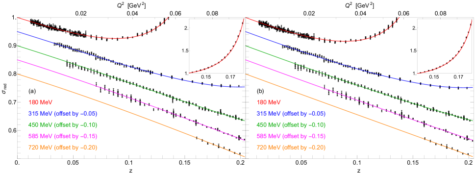
Figure 1: (Color online) Fits to the low-$Q^{2}$ data of Ref. Bernauer et al. (2010) using single-parameter models for the form factors in Eq. (1). In (a), the dipole model of Eq. (3) is used, and in (b) the linear model of Eq. (5) is used. Separate plots are required since the fits return different normalization constants, and therefore the cross sections take on slightly ($\sim$1%) different values for the two plots. The $E$=180 MeV data and fits are continued in the insets, and the other energies are offset for clarity of presentation.

The highest-accuracy e-p scattering experiment Bernauer et al. (2010) by the MAMI collaboration yields 1422 cross sections (with typical relative uncertainties of 0.35%) spanning a range of 180 MeV $\leq E\leq$855 MeV and 16${}^{\circ}\leq\theta\leq 135.5^{\circ}$, corresponding to 0.0038 GeV${}^{2}<Q^{2}<$ 1 GeV² and $0.06<\epsilon<1$. The 1422 cross sections are divided into 34 data groups, with each data group having a separate normalization constant. These normalization constants are known to an absolute accuracy of a few percent, and are related to one another in such a way that there are only 31 independent constants Bernauer et al. (2010, 2014); *BernauerThesis.

The normalization constants add a further complication to the $Q^{2}$=0 extrapolation needed to determine $R_{\rm E}$. The few-percent absolute accuracy of the measured cross sections is not sufficient for performing a precise extrapolation, and thus the 31 normalization constants need to be floated when performing least-squares fits of the entire data set for this extrapolation. We include these normalization constants in all of our fits. Floating these constants adds considerable flexibility to the extrapolations. Although we do not impose the few-percent absolute uncertainty of the normalization constants in our fits, all of our fits return constants near unity and well within this few-percent uncertainty.

Other least-squares fits Bernauer et al. (2010, 2014); *BernauerThesis; Lorenz and Meißner (2014); Lorenz et al. (2015); Lee et al. (2015); Lorenz et al. (2012) of this data use seven- to twelve-parameter models for $G_{\rm E}$ and for $G_{\rm M}$, and obtain least-squares fits with reduced $\chi^{2}$ values of as low as 1.14 for fitting the 1422 data points. The 1.14 value is much too large for the number of degrees of freedom in the fit, but can easily be explained by either a 7% underestimation of the uncertainties, or a systematic effect that is not fully accounted for. We only include fits that have a reduced $\chi^{2}$$<$1.14 in this work.

As indicated by Eq. (2), the rms charge radius of the proton is a small-$Q^{2}$ concept. Thus, if possible, it should be determined from low-$Q^{2}$ data. Therefore, we attempt to make a determination of $R_{\rm E}$ using fits to only the lower-$Q^{2}$ data. In addition to the fact that such fits use data nearer to $Q^{2}$=0, the fits have the advantages that simpler, fewer-parameter models can be used for $G_{\rm E}^{2}$ and $G_{\rm M}^{2}$, and that, since fewer of the data groups are used, fewer normalization constants need to be included in the fits.

Fits using single-parameter models for the form factors are shown in Fig. 1. These fits include data with $Q^{2}$$\leq$$Q^{2}_{\rm max}$=0.1 GeV², from 19 data groups, which require 17 normalization constants. A data group is only included if there are more than 10 data points in the group, and a total of 761 of the 1422 cross sections (53%) are used. The value of $R_{\rm E}$ is directly obtainable from the slope of the curves in Fig. 1 at $Q^{2}$=0, and the fits provide the necessary extrapolation to $Q^{2}$=0.

Fig. 1(a) shows a fit using Eq. (1) and the one-parameter dipole form factors of Eq. (3). The reduced $\chi^{2}$ for the fit is 1.11, and the fit returns $R_{\rm E}$=$(12/b_{E})^{1/2}$=0.842(2) fm and $R_{\rm M}$=$(12/b_{M})^{1/2}$ =0.800(2) fm.

A second fit to the same data uses the one-parameter linear model (in $z$) of Eq. (5). This fit is shown in Fig. 1(b). It also has a reduced $\chi^{2}$ of 1.11 and gives $R_{\rm E}$=$(\frac{3}{4}c_{\rm E}/t_{c})^{1/2}$=0.888(1) fm and $R_{\rm M}$=$(\frac{3}{4}c_{\rm M}/t_{c})^{1/2}$=0.874(2) fm.

Figure 2 shows (red bands labeled Eq. (3) and Eq. (5) at the left of the figure) the error bands for $R_{\rm E}$ for the dipole and linear fits versus the cutoff $Q_{\rm max}^{2}$. The figure includes the range of $Q_{\rm max}^{2}$ for which a reduced $\chi^{2}$$<$1.14 is obtained.

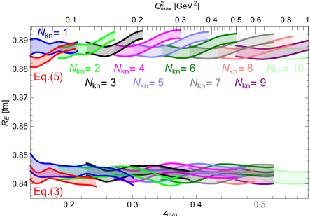
Figure 2: (Color online) The range of $R_{\rm E}$ predicted from the dipole fits (lower bands) and conformal-mapping fits (upper bands) as a function of the cutoff value $Q_{\rm max}^{2}$. The red bands correspond to single-parameter dipole and linear fits of Eqs. (3) and (5), and the other colors show extensions to these fits for which the single parameters are replaced with cubic splines (with the number of nodes, $N_{\rm kn}$, as indicated) at larger $Q^{2}$. All fits shown have a reduced $\chi^{2}$$<$1.14.

The electric form factors predicted from the two fits of Fig. 1 are shown in Fig. 3. Also plotted in the figure are other low-$Q^{2}$ measurements of these form factors (often referred to as the world data, as summarized in Ref. Arrington et al. (2007)). It is clear from this figure (and from the calculated $\chi^{2}$ for the comparison betwen the data and the two curves) that the form factor from either fit is also consistent with these other measurements.

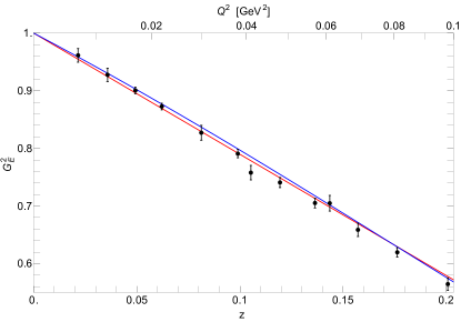
Figure 3: (Color online) Electric form factor $G_{\rm E}$ determined from the single-parameter fits of Fig 1. The blue curve is from the dipole-model fit, and the red curve is from the linear-model fit. Also shown on the plots are the low-$Q^{2}$ $G_{\rm E}$ data from other experiments (from Arrington et al. (2007)), and these data are consistent with the $G_{\rm E}$ obtained from either fit.

One concern that could be raised about the single-parameter fits, which are based only on data with $Q^{2}<Q_{\rm max}^{2}$, is that they may lead to inconsistencies for data with $Q^{2}$$>$$Q_{\rm max}^{2}$. Since the low-$Q^{2}$ fits of Fig. 1 determine 17 of the 31 normalization constants, and since data groups using these normalization constants include measured cross sections with $Q^{2}>Q_{\rm max}^{2}$, the fits have a direct impact on data not included when fitting. It could, therefore, be possible that data at the same value of $Q^{2}>Q_{\rm max}^{2}$ from two of these data groups could be made inconsistent when these normalization constants are used.

To ensure that such inconsistencies do not take place, we extend the fits of the previous section to include all of the MAMI data. Such an extension also allows for a direct comparison of the quality of our fits to the quality of the fits performed by others Bernauer et al. (2010, 2014); *BernauerThesis; Lorenz and Meißner (2014); Lorenz et al. (2015); Lee et al. (2015); Lorenz et al. (2012) who also include all of the MAMI data. The extended fits include a range of $Q^{2}$ in which the functional form of $G_{\rm E}^{2}$ and $G_{\rm M}^{2}$ becomes more complicated, and, as with the fits performed by others, more parameters are necessary to obtain a good fit.

The fit using Eq. (3) can be generalized by allowing the constants $b_{\rm E}$ and $b_{\rm M}$ to become functions of $z$. We do this by using cubic splines, with the $b$ values each being a constant for $z<z_{\rm 0}$=0.1, and with $N_{\rm kn}$ equally spaced knots between $z_{\rm 0}$ and $z_{\rm max}$. The values of $b$, and their first and second derivatives are continuous at $z_{\rm 0}$ and at the other knots. The number of knots needed to achieve a good fit increases with increasing $z_{\rm max}$.

The results of such fits with $N_{\rm kn}$=1 to 10 (2 to 11 parameters per form factor) are given in Fig. 2. Again, only fits with a reduced $\chi^{2}$$<$1.14 are shown. The fits return values of $R_{\rm E}$ of approximately 0.84 fm for all values of $Q^{2}_{\rm max}$, similar to the single-parameter dipole fit. The fits at the right of the plot include all of the MAMI data, and still return a value near 0.84 fm.

Equation (5) would predict negative values for $G_{\rm E}^{2}$ and $G_{\rm M}^{2}$ at larger $z$. This problem can be avoided by using a denominator to cause a cutoff at higher $z$ values:

$$G_{\rm E}^{2}=\frac{1-c_{\rm E}z}{1-(c_{\rm E}z)^{P}}\ {\rm and}\ \frac{G_{\rm M}^{2}}{\mu_{\rm p}^{2}}=\frac{1-c_{\rm M}z}{1-(c_{\rm M}z)^{P}}.$$ (6)

We use $P$=4 for our fits, but any $P$ from 4 to 14 gives similar results. This function is very nearly linear up to $z$=0.2, while avoiding negative values at larger $z$. A fit of the data to these form factors is performed by allowing $c_{\rm E}$ and $c_{\rm M}$ to become functions of $z$ by using the same form of cubic splines as are used for $b_{\rm E}$ and $b_{\rm M}$.

The results of such fits with $N_{\rm kn}$=1 to 10 are also given in Fig. 2. The fits return values of $R_{\rm E}$ of approximately 0.89 fm, similar to the single-parameter linear fit.

Fig. 2 clearly indicates that the two types of fits produce values of $R_{\rm E}$ that disagree with each other. Since either type of fit gives an extrapolation to zero $Q^{2}$ that is equally valid, and since the quality of the fits are similar, either value of $R_{\rm E}$ is possible. Therefore, at best, the determined value of $R_{\rm E}$ can range from 0.84 to 0.89 fm. At worst, other valid extrapolations could lead to even a wider range of possible values, leading to an even larger range for $R_{\rm E}$.

It is not the aim of this work to determine the rms magnetic radius of the proton, $R_{\rm M}$, but we note that the values from our fits range from about 0.80 to 0.90 fm, and therefore this work cannot determine $R_{\rm M}$ to any better than this range. The consistency of the fits presented in this work can be checked by comparing the quantity $R_{\rm E}^{2}+R_{\rm M}^{2}$ to the prediction from hydrogenic spectroscopy. The hydrogen hyperfine interval determines $R_{\rm E}^{2}+R_{\rm M}^{2}$ to be 1.35(12) fm², and the muonic hydrogen hyperfine interval determines $R_{\rm E}^{2}+R_{\rm M}^{2}$ to be 1.49(18) fm² Karshenboim (2014). The two determinations are consistent, and their weighted average gives $R_{\rm E}^{2}+R_{\rm M}^{2}$ = 1.39(10) fm². The dipole fit of Fig. 1(a) gives $R_{\rm E}^{2}+R_{\rm M}^{2}$ = 1.349(4), whereas the linear fit of Fig. 1(b) gives 1.553(4). The dipole fit is in excellent agreement with the spectroscopy result, and the linear fit shows only a mild 1.6 standard deviation discrepancy. Similar comparisons using the extended cubic-spline fits lead to a similar level of agreement.

The extent to which two-photon exchange (TPE) affects the extraction of $R_{\rm E}$ from the MAMI data has been debated in the literature Arrington (2011); Bernauer et al. (2011, 2014); *BernauerThesis; Pohl et al. (2013); Lee et al. (2015); Rachek et al. (2015); Nikolenko et al. (2015); Tomalak and Vanderhaeghen (2015a); Borisyuk and Kobushkin (2015); Tomalak and Vanderhaeghen (2015b); Arrington (2013); Adikaram et al. (2015). The cross sections given in Ref. Bernauer et al. (2014); *BernauerThesis were corrected by the Coulomb corrections (Feshbach corrections McKinley Jr and Feshbach (1948)) in place of the full TPE corrections. In this work, these Coulomb corrections are removed and and replaced with TPE corrections calculated following the prescription of Borisyuk and Kobushkin (2012a, b). This replacement leads to correction factors of between 0.997 and 1.003 for the data of Fig. 1, and of between 0.978 and 1.003 for the full MAMI set. The correction factors agree with those shown in Fig. 5 of Ref. Lorenz et al. (2015) to within the 0.03% accuracy readable from their figure. To test how sensitive our analysis is to TPE corrections, we repeat our full analysis using the low-$Q^{2}$ TPE approximation of Ref. Borisyuk and Kobushkin (2007) and the Feshbach correction in place of the full TPE correction. Fig. 4 shows that using the Feshbach correction would underestimate $R_{\rm E}$ by only 0.004 fm, while the low-$Q^{2}$ approximation would change $R_{\rm E}$ by less than 0.001 fm. We conclude that, although the best available TPE corrections should be used, the sensitivity to using poorer approximations is small in our analysis.

In summary, we have reanalyzed electron-proton elastic scattering data using simple fits to the lowest-$Q^{2}$ half of the data, and cubic-spline extensions of these fits at higher $Q^{2}$. We find that the required extrapolation to $Q^{2}$=0 can lead to values for the rms charge radius $R_{\rm E}$ ranging from 0.84 to 0.89 fm. This range does not resolve the discrepancy between determinations of $R_{\rm E}$ from muonic hydrogen Pohl et al. (2010); Antognini et al. (2013) and ordinary hydrogen Mohr et al. (2012).

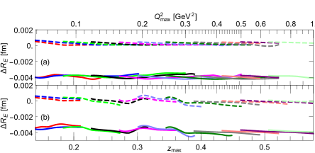
Figure 4: (Color online) The sensitivity of the fit results of Fig. 2 to two-photon exchange corrections is illustrated by redoing the analysis with poorer approximations for these corrections. The change in $R_{\rm E}$ when the Feshbach corrections (solid curves) and a low-$Q^{2}$ approximation Borisyuk and Kobushkin (2007) (dashed curves) are applied shows that the radius extracted from both the dipole model (a) and conformal-mapping model (b) is not very sensitive to these corrections.

This work is supported by NSERC and CRC.

References

- Pohl et al. (2010) R. Pohl, A. Antognini, F. Nez, F. D. Amaro, F. Biraben, J. M. Cardoso, D. S. Covita, A. Dax, S. Dhawan, L. M. Fernandes, et al., Nature 466, 213 (2010).
- Antognini et al. (2013) A. Antognini, F. Nez, K. Schuhmann, F. D. Amaro, F. Biraben, J. M. Cardoso, D. S. Covita, A. Dax, S. Dhawan, M. Diepold, et al., Science 339, 417 (2013).
- Mohr et al. (2012) P. J. Mohr, B. N. Taylor, and D. B. Newell, Journal of Physical and Chemical Reference Data 41, 043109 (2012).
- Bernauer et al. (2010) J. C. Bernauer, P. Achenbach, C. Ayerbe Gayoso, R. Böhm, D. Bosnar, L. Debenjak, M. O. Distler, L. Doria, A. Esser, H. Fonvieille, J. M. Friedrich, J. Friedrich, M. Gómez Rodríguez de la Paz, M. Makek, H. Merkel, D. G. Middleton, U. Müller, L. Nungesser, J. Pochodzalla, M. Potokar, S. Sánchez Majos, B. S. Schlimme, S. Širca, T. Walcher, and M. Weinriefer, Phys. Rev. Lett. 105, 242001 (2010).
- Bernauer et al. (2014) J. Bernauer, M. Distler, J. Friedrich, T. Walcher, P. Achenbach, C. A. Gayoso, R. Böhm, D. Bosnar, L. Debenjak, L. Doria, et al., Physical Review C 90, 015206 (2014).
- (6) J. C. Bernauer, Dissertation, Johannes Gutenberg-Universität, Mainz, 2010.
- Bernauer and Pohl (2014) J. C. Bernauer and R. Pohl, Scientific American 310, 32 (2014).
- Note (1) See reviews of these discussions in Refs. Carlson (2015) and Pohl et al. (2013).
- Arrington (2011) J. Arrington, Phys. Rev. Lett. 107, 119101 (2011).
- Bernauer et al. (2011) J. C. Bernauer, P. Achenbach, C. Ayerbe Gayoso, R. Böhm, D. Bosnar, L. Debenjak, M. O. Distler, L. Doria, A. Esser, H. Fonvieille, J. M. Friedrich, J. Friedrich, M. Gómez Rodríguez de la Paz, M. Makek, H. Merkel, D. G. Middleton, U. Müller, L. Nungesser, J. Pochodzalla, M. Potokar, S. Sánchez Majos, B. S. Schlimme, S. Širca, T. Walcher, and M. Weinriefer (A1 Collaboration), Phys. Rev. Lett. 107, 119102 (2011).
- Lorenz et al. (2012) I. Lorenz, H.-W. Hammer, and U.-G. Meißner, The European Physical Journal A 48, 1 (2012).
- Sick (2012) I. Sick, Progress in Particle and Nuclear Physics 67, 473 (2012).
- Pohl et al. (2013) R. Pohl, R. Gilman, G. A. Miller, and K. Pachucki, Annual Review of Nuclear and Particle Science 63, 175 (2013).
- Adamuščín et al. (2013) C. Adamuščín, E. Bartoš, S. Dubnička, and A. Dubničková, Nuclear Physics B-Proceedings Supplements 245, 69 (2013).
- Kraus et al. (2014) E. Kraus, K. Mesick, A. White, R. Gilman, and S. Strauch, Physical Review C 90, 045206 (2014).
- Lorenz and Meißner (2014) I. Lorenz and U.-G. Meißner, Physics Letters B 737, 57 (2014).
- Lorenz et al. (2015) I. Lorenz, U.-G. Meißner, H.-W. Hammer, and Y.-B. Dong, Physical Review D 91, 014023 (2015).
- Carlson (2015) C. E. Carlson, Progress in Particle and Nuclear Physics 82, 59 (2015).
- Lee et al. (2015) G. Lee, J. R. Arrington, and R. J. Hill, Phys. Rev. D 92, 013013 (2015).
- Arrington and Sick (2015) J. Arrington and I. Sick, Journal of Physical and Chemical Reference Data 44, 031204 (2015).
- Pacetti et al. (2015) S. Pacetti, R. B. Ferroli, and E. Tomasi-Gustafsson, Physics Reports 550, 1 (2015).
- Arrington et al. (2011) J. Arrington, P. Blunden, and W. Melnitchouk, Progress in Particle and Nuclear Physics 66, 782 (2011).
- Note (2) See, for example, L. N. Hand, D. G. Miller, and R. Wilson, Rev. Mod. Phys. 35, 335 (1963).
- Hill and Paz (2010) R. J. Hill and G. Paz, Physical Review D 82, 113005 (2010).
- Arrington et al. (2007) J. Arrington, W. Melnitchouk, and J. A. Tjon, Phys. Rev. C 76, 035205 (2007).
- Karshenboim (2014) S. G. Karshenboim, Phys. Rev. D 90, 053013 (2014).
- Rachek et al. (2015) I. Rachek, J. Arrington, V. Dmitriev, V. Gauzshtein, R. Gerasimov, A. Gramolin, R. Holt, V. Kaminskiy, B. Lazarenko, S. Mishnev, et al., Physical Review Letters 114, 062005 (2015).
- Nikolenko et al. (2015) D. Nikolenko, J. Arrington, L. Barkov, H. de Vries, V. Gauzshtein, R. Golovin, A. Gramolin, V. Dmitriev, V. Zhilich, S. Zevakov, et al., Physics of Atomic Nuclei 78, 394 (2015).
- Tomalak and Vanderhaeghen (2015a) O. Tomalak and M. Vanderhaeghen, arXiv preprint arXiv:1508.03759 (2015a).
- Borisyuk and Kobushkin (2015) D. Borisyuk and A. Kobushkin, Physical Review C 92, 035204 (2015).
- Tomalak and Vanderhaeghen (2015b) O. Tomalak and M. Vanderhaeghen, The European Physical Journal A 51, 1 (2015b).
- Arrington (2013) J. Arrington, Journal of Physics G: Nuclear and Particle Physics 40, 115003 (2013).
- Adikaram et al. (2015) D. Adikaram, D. Rimal, L. Weinstein, B. Raue, P. Khetarpal, R. Bennett, J. Arrington, W. Brooks, K. Adhikari, A. Afanasev, et al., Physical Review Letters 114, 062003 (2015).
- McKinley Jr and Feshbach (1948) W. A. McKinley Jr and H. Feshbach, Physical Review 74, 1759 (1948).
- Borisyuk and Kobushkin (2012a) D. Borisyuk and A. Kobushkin, Physical Review C 86, 055204 (2012a).
- Borisyuk and Kobushkin (2012b) D. Borisyuk and A. Kobushkin, arXiv preprint arXiv:1209.2746 (2012b).
- Borisyuk and Kobushkin (2007) D. Borisyuk and A. Kobushkin, Physical Review C 75, 038202 (2007).