Abstract. We describe a numerical model of faceted crystal growth using a cellular automata method that incorporates admolecule diffusion on faceted surfaces in addition to bulk diffusion in the medium surrounding the crystal. The model was developed for investigating the diffusion-limited growth of ice crystals in air from water vapor, where the combination of bulk diffusion and strongly anisotropic molecular attachment kinetics yields complex faceted structures. We restricted the present model to cylindrically symmetric crystal growth with relatively simple growth morphologies, as this was sufficient for making quantitative comparisons between theoretical models and ice growth experiments. Overall this numerical model reproduces ice growth behavior with reasonable fidelity over a wide range of conditions, albeit with some limitations. The model could easily be adapted for other material systems, and the cellular automata technique appears well suited for investigating crystal growth dynamics when strongly anisotropic surface attachment kinetics cause faceted growth morphologies.

1 Introduction

The formation of crystalline structures during solidification yields a remarkable variety of morphological behaviors, resulting from the often subtle interplay of non-equilibrium physical processes over a range of length scales. In many cases, seemingly small changes in surface molecular structure and dynamics at the nanoscale can produce large morphological changes at all scales. Some examples include free dendritic growth from the solidification of melts, where small anisotropies in the interfacial surface energy govern the overall characteristics of the growth morphologies [1, 2], whisker growth from the vapor phase initiated by single screw dislocations and other effects [3], the formation of porous aligned structures from directional freezing of composite materials [4], and a range of other pattern formation systems [5, 6]. Since controlling crystalline structure formation during solidification has application in many areas of materials science, much effort has been directed toward better understanding the underlying physical processes and their interactions.

We have been exploring the growth of ice crystals from water vapor in an inert background gas as a case study of how complex faceted structures emerge in diffusion-limited growth. Although this is a relatively simple monomolecular physical system, ice crystals exhibit columnar and plate-like growth behaviors that depend strongly on temperature, and much of the phenomenology of their growth remains poorly understood [7, 8, 9]. Ice has also become something of a standard test system for investigating numerical methods of faceted crystal growth [10, 11, 12, 13]. A better understanding of ice crystal formation yields insights into the detailed molecular structure and dynamics of the ice surface, which in turn contributes to our understanding of many meteorological, biological, and environmental processes involving ice [14, 15, 16].

In our investigation of how surface energy and attachment kinetics affect ice growth dynamics, we needed a quantitative numerical model that would allow us to “grow” model ice crystals for comparison with experimental measurements of growth rates and morphologies. Although proven numerical methods for modeling diffusion-limited growth have been available for years, many of the existing methods are ill-suited for modeling ice growth behavior. For example, phase-field [17, 18] and front-tracking [19] methods have demonstrated the ability to accurately model diffusion-limited growth for the case of fast attachment kinetics and a weakly anisotropic surface energy, which is characteristic of most solidification from the melt. These systems typically yield unfaceted dendritic structures, however, in contrast to strongly faceted ice structures. Early models for the growth of faceted crystals [20, 21] were generally too limited to allow quantitative comparisons with ice growth data.

Modeling diffusion-limited growth in systems with strong surface anisotropies has proven difficult, and only recently have researchers demonstrated robust techniques capable of generating structures that are both faceted and dendritic. Reiter [10] described an especially promising cellular automata simulator that solves the diffusion equation by nearest neighbor relaxation, including a set of parameterized nearest neighbor rules to define the boundary conditions at the crystal interface. This model was further advanced by several researchers [22, 23, 11, 24, 25, 13], and the method yields a deterministic dendritic growth behavior in which faceting follows the symmetry of the predefined numerical grid.

Barrett et al. [12] also developed a robust adaptive mesh technique that generated faceted dendritic crystal growth patterns. In this work the authors found that a strongly anisotropic surface energy was required to produce faceted dendritic growth, while anisotropic attachment kinetics alone were not sufficient to reproduce this behavior. We have suggested that the ice case is more likely described by the opposite characteristics – a nearly isotropic surface energy together with strongly anisotropic attachment kinetics, the latter dominating the growth behavior [26]. In fact, the roles played by these two physical effects are not yet known with certainty.

The relative merits of different computational methods for modeling diffusion-limited growth in the presence of strong surface anisotropies are not presently well understood, as this is an area of current research. Moreover, our knowledge of the surface physics governing the growth of faceted materials is itself rather poor, including the relative contributions of the anisotropies in surface energy and attachment kinetics in different materials. In our experience, progress on both these research fronts is linked: better modeling methods allow more accurate interpretation of growth experiments, in turn fostering improved experiments that yield a better understanding of the surface physics input into the models.

Below we describe a cellular automata method for modeling diffusion-limited growth in the presence of strongly anisotropic molecular attachment kinetics, focusing on ice growth from water vapor. The model is an extension of that presented in [25], now including admolecule diffusion on faceted surfaces, which is quite important when vicinal surfaces are present. While we are not yet able to reproduce all aspects of faceted growth behavior, our model is robust, numerically well-behaved, computationally straightforward, and quite flexible for exploring ice growth behaviors.

The 2D cylindrically symmetric model has been especially useful for investigating the simple growth morphologies often produced in experiments. A basic hexagonal prism, for example, is modeled by a right cylinder, replacing the six prism facets with a single cylindrical “facet”. This model is adequate for basic plate and needle morphologies, as well as some more complex forms such as capped columns, hollow columns, and double plates. Using a 2D model allows the rapid generation of hundreds of model crystals for comparison with experimental results, using different input assumptions. We have found that this model is quite useful when examining the surface physical processes governing ice growth rates, and it allows straightforward adaptation for use in other investigations involving faceted diffusion-limited crystal growth.

2 Incorporating Surface Diffusion

The new model presented here is a direct extension of what we described in detail in [25], so we will not reproduce a derivation of the physics underlying the central features of the cellular automata method. We reiterate, however, that our overarching goal in this effort has been to define a physically accurate crystal growth model for quantitative comparison with crystal growth experiments. Thus we strive to model not only the correct faceted crystal morphologies, but correct crystal growth rates as well. This is in contrast to several earlier cellular automata models of ice growth [10, 22, 23, 11], in which particle diffusion in the medium surrounding the crystal was treated correctly, but with somewhat ad hoc surface boundary conditions.

To date, all the cellular automata models of ice crystal growth have incorporated local surface boundary conditions. In these models, the boundary conditions to the bulk diffusion equation at a given point on the ice surface depend only on conditions at that point, and are independent of processes occurring at other surface locations. Such local models do not include admolecule diffusion on faceted surfaces, as surface transport is a nonlocal process. As described in [25], we previously assumed that surface diffusion processes that act over length scales of order $x_{s},$ the surface diffusion length [27], could be incorporated into the local attachment coefficient $\alpha,$ as long as the model resolution was restricted to length scales greater than $x_{s}.$ We next show that this assumption was incorrect.

2.1 A Microscopic Model

Before examining the effects of surface diffusion in our macroscopic cellular automata model, we first define an appropriate molecular model of the process [27]. Note that our model of surface diffusion is independent of the bulk diffusion taking place in the medium surrounding the crystal. In our physical picture of ice crystal growth from water vapor, both diffusion processes are present: water molecules first diffuse through the air to reach the ice crystal surface, and subsequently diffuse along the crystal surface before becoming incorporated into the crystal lattice. (Heat diffusion from latent heat deposition at the growing surface is neglected for the reasons stated in [7].) We consider only admolecule diffusion on faceted surfaces. On rough surfaces, we retain the assumption that admolecules are immediately incorporated into the lattice, so the attachment coefficient is $\alpha\approx 1$ on nonfaceted surfaces.

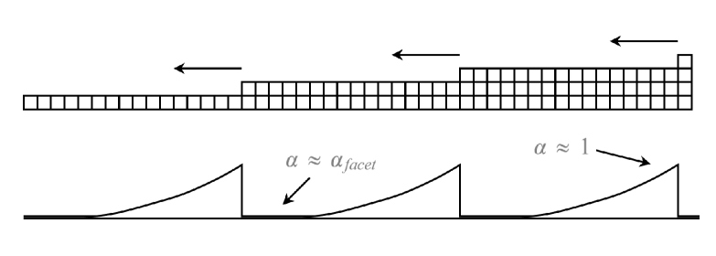
Figure 1: A basic molecular model of surface diffusion, here depicted in 2D $(r,z)$ space. The boxes in the upper diagram represents water molecules, collectively showing a cut-away side view of a vicinal surface. The curve below indicates the attachment coefficient $\alpha$ along the surface. As described in the text, $\alpha\approx\alpha_{facet}$ far from kink sites, while $\alpha\approx 1$ near kink sites. In this sketch the diffusion distance $x_{s}$ is just a few molecules wide, while in reality $x_{s}$ may be much larger. As the crystal grows, water molecules attach to the kink sites, so the edge of each terrace advances to the left.

To examine surface diffusion in detail, consider a simple vicinal surface, on which a series of molecular terrace steps are separated by a uniform spacing $x_{step}$, as shown in Figure 1. Let $x_{s}$ equal the usual surface diffusion length [27], equal to the typical distance admolecules diffuse during their residence time on the surface. We assume for the present discussion that the Ehrlich–Schwoebel barrier reduces admolecule diffusion over terrace steps to a negligible rate. If $x_{step}\ll x_{s}$, then essentially all admolecules will diffuse to kink sites and be absorbed, contributing to crystal growth. The attachment coefficient for such a vicinal surface is then $\alpha\approx 1;$ all molecules that strike the surface become incorporated into the crystal lattice.

If $x_{step}\gg x_{s},$ then only admolecules within a distance approximately $x_{s}$ from each step will be absorbed, and $\alpha<1$ when averaged over the surface. More specifically, we define an attachment coefficient arising from surface diffusion as $\alpha_{SD}\approx\exp(-\Delta x/x_{x}),$ where $\Delta x$ is the distance to an accessible kink site [27], as shown in Figure 1. For a faceted surface near a terrace step, therefore, we must consider both $\alpha_{SD}$ and $\alpha_{facet},$ the latter being the intrinsic attachment coefficient for a perfectly faceted surface.

Is is useful to frame this molecular process in the language of a cellular automata model [25], taking the cells in Figure 1 to be molecule-size pixels in the numerical model. To include surface diffusion in this model, we should: 1) include $\alpha_{SD}$ on facet sites that are near kink sites, and 2) transfer the additional accumulated mass $dM$ – that part arising from surface diffusion – to the appropriate kink sites. (See [25] for a definition of the accumulated mass in the cellular automata model.)

In our numerical testing of this model, we have found that item (2) can be ignored without substantially changing the growth rate or morphological behavior. Making the assumption $\alpha_{SD}=\exp(-\Delta x/x_{s})$ from surface diffusion at each point along the surface, with no mass transport to kink sites, models the growth rate with reasonable fidelity. The reason for this is that adding $dM$ just ahead of a moving kink site gives essentially the same numerical result as transporting the same $dM$ to the kink site. The key element of surface diffusion in our model is to increase $\alpha$, and thus increase $dM,$ near kink sites.

The value of $x_{s}$ on faceted ice surfaces is not well known. In [28], the authors reported $x_{s}\approx 5$ $\mu$m for the diffusion length on a basal facet at -8 C; however the same data were reinterpreted in [29] to obtain a value $x_{s}\approx 10$ nm. This is an area of active research, and there is a clear need for additional measurements. Nevertheless, for vicinal surfaces tilted by angles as low as $\theta\approx a/x_{s}$ we can effectively assume $\alpha\approx 1$ on the surface. Since $\alpha_{facet}$ can be quite small when $\theta=0,$ a large $x_{s}$ would mean that that $\alpha\left(\theta\right)$ exhibits an extremely sharp cusp at $\theta=0,$ pinpointing the difficulty inherent in modeling faceted crystal growth.

2.2 The Macroscopic Model

We next apply this physical picture of surface diffusion to our 2D cylindrically symmetric model in $(r,z)$ space [25], which has pixels that are typically $\Delta r=\Delta z\approx 0.15$ $\mu$m in size. Our numerical algorithm for surface diffusion is essentially that described in Figure 1 for the microscopic model. For each faceted boundary pixel we calculate $\alpha_{SDleft}$ and $\alpha_{SDright}$ representing the accumulated mass absorbed by kink sites on either side of a particular facet site. If there is no kink site in one or both directions, then the appropriate $\alpha_{SDx}$ values are zero. Specifically, for each facet site we take

$$\alpha_{SDleft} = A_{SD}\exp(-\Delta n_{left}/n_{SD})$$

$$\alpha_{SDright} = A_{SD}\exp(-\Delta n_{right}/n_{SD})$$

where $\Delta n_{left}$ and $\Delta n_{right}$ are the distances to accessible kink sites (if they exist) on either side of the facet site, in pixels. For basal facets (in our 2D model), the $\Delta n_{x}$ are pixel distances in the $r$ direction from the facet site in question; for prism facets, the $\Delta n_{x}$ are pixel distances in the $z$ direction. The constant $A_{SD}$ is typically set to unity, but we leave it as an adjustable parameter in our model.

Our choice for $n_{SD}$ follows from the discussion of vicinal angles above, from which we obtain $n_{SD}=(x_{s}/a)$ pixels. With this value for $n_{SD},$ we have $\alpha_{SD}\approx A_{SD}\approx 1$ whenever a vicinal surface is tilted by an angle greater than $\theta\approx 1/n_{SD}\approx a/x_{s},$ the same angle as we found above. By this straightforward equal-angle argument, we see that the effects of surface diffusion do not extend to $x_{s}/\Delta z$ pixels, as one might naively assume, but a factor of $(\Delta z/a)\approx 500$ times farther. This additional factor of $(\Delta z/a)$ is a key result in this paper, as it shows the importance of including surface diffusion in a cellular automata model of ice growth.

At this point we can see a possibly important limitation in our numerical model. With a spatial resolution of $\Delta z,$ vicinal surfaces with $\theta<\Delta z/L$ will be indistinguishable from perfectly faceted surfaces, where $L$ is the overall size of the facet. Such surfaces will have no $\Delta z$ steps in the model, so must have $\alpha=\alpha_{facet}\ll 1,$ In reality, however, the vicinal angle must go to $\theta<a/L\ll\Delta z/L$ before $\alpha=\alpha_{facet}.$ If $x_{s}$ is large, this means our model will have difficulty modeling nearly faceted surfaces, which we will discuss in more detail below.

To complete our numerical algorithm of surface diffusion, we compute a total $\alpha_{SD}$ at each facet site using

$$\alpha_{SD} = \alpha_{SDleft}+\alpha_{SDright}-\alpha_{SDleft}\alpha_{SDright}$$

$$= C(\alpha_{SDleft},\alpha_{SDright})$$

(We note in passing that $\alpha_{SD}$ is calculated from the crystal geometry alone, independent of the supersaturation field surrounding the crystal.) We also compute $\alpha_{facet}$ for each facet site, which generally depends on the surface supersaturation $\sigma_{surf}$, and this is combined with $\alpha_{SD}$ to form the total attachment coefficient $\alpha_{tot}=C(\alpha_{facet},\alpha_{SD})$. This addition of $\alpha$ terms follows from the “at least one” rule for combining independent probabilities, the general case being

$$p_{tot}=1-\prod_{i}(1-p_{i})$$

(M. Libbrecht, private communication). The reader can verify that this rule gives the expected results for $\alpha_{tot}$ in various limits. For example, $\alpha_{tot}\approx 1$ on the lower terrace near a step, $\alpha_{tot}\approx\alpha_{facet}$ far from any step, and $\alpha_{tot}\approx 1$ independent of $\alpha_{SD}$ if $\alpha_{facet}\approx 1$.

The result of including this surface diffusion algorithm can be seen by considering the top sketch in Figure 1, this time interpreting the cells as pixels in the cellular automata model. Atop the highest terrace on the facet surface, which we call the “top terrace”, we still have $\alpha=\alpha_{facet},$ because there are no accessible kink sites (owing to our initial assumption of a large Ehrlich–Schwoebel barrier). At all other sites, $\alpha_{tot}$ is much increased, typically to $\alpha_{tot}\approx 1$ everywhere except on the top terraces (because $n_{SD}=(\Delta z/a)x_{s}\approx 500\$pixels is typically larger than the crystals we are modeling, so $\exp(-\Delta n_{left}/n_{SD})\approx 1)$. This is in contrast to our previous model without surface diffusion [25], where we had $\alpha=\alpha_{facet}$ on all facet sites and $\alpha=1$ only on kink sites.

We can see how the addition of surface diffusion in our model promotes faceting in two ways. First, lower terrace sites have larger $\alpha$ values and thus grow more quickly. Second, the larger $\alpha$ values decrease the $\sigma$ field everywhere around the crystal, including on the top terrace. Because $\alpha_{facet}$ typically depends strongly on $\sigma_{surf},$ this lowers $\alpha_{facet}$ and thus reduces the nucleation of new terraces on the top terrace. Thus the lower terraces fill in more quickly, while nucleation of new terraces is reduced. These two factors both lead to increased faceting.

3 The 2D Cellular Automata Model

It is beneficial at this point to describe the flow through our numerical model in some detail. Here again, the reader can find the derivation of many of the algorithms below described in [25].

3.1 Attachment Coefficients

The intrinsic attachment coefficients for faceted prism and basal facets are typically parameterized by $\alpha_{facet}=A\exp(-\sigma_{0}/\sigma_{surf})$. where $\sigma_{surf}$ is the supersaturation at the surface. The parameters $A$ and $\sigma_{0}$ are different for the basal and prism facets, and will generally depend on temperature, but they do not depend on $\sigma_{surf}$. We have measured $A(T)$ and $\sigma_{0}(T)$ over a fairly broad range of temperatures for the two facets [30], but we often vary their values when investigating ice growth rates from other experiments. We typically assume $\alpha=1$ for all nonfaceted surface boundary pixels.

On the outermost facet surfaces (the top basal and prism terraces), we reduce the supersaturation by the Gibbs-Thomson effect to

$$\sigma_{surf}\rightarrow\sigma_{surf}-\frac{\delta}{R}$$

where $R$ is an effective curvature term defined in [25]. Our code makes a rather crude estimate of $R,$ only applied to the outermost faceted surfaces, since we have not yet found a satisfactory algorithm for estimating the surface curvature of complex structures in cellular automata. We believe that the Gibbs-Thomson effect is negligible in many typical experimental circumstances, but we include it mainly to suppress the growth of one-pixel-wide structures at low supersaturations, as described in [25].

3.2 Initial Relaxation

After defining the seed crystal geometry and other parameters, our model first calculates the supersaturation field $\sigma\left(r,z\right)$ around the crystal. We assume a simple outer boundary condition $\sigma=\sigma_{\infty}$, where $\sigma_{\infty}$ is a constant input parameter. For pixels not on the crystal boundary, we iterate the relaxation equation

$$\sigma(\tau+\Delta\tau)=\Delta\tau\left[f_{-}(r)\sigma(r-\Delta r)+f_{+}(r)\sigma(r+\Delta r)+\sigma(z-\Delta z)+\sigma(z+\Delta z)\right]$$

to solve the Laplacian, where $\Delta\tau=1/4$ and

$$f_{\pm}(r)=\left(1\pm\frac{\Delta r}{2r}\right)$$

as described in [25]. This step is applied by shifting the $\sigma(r,z)$ matrix by one pixel in $\pm r$ and $\pm z$, and then adding the results, handling everything in full matrix form for better computational efficiency. Special handling of the $r=0$ and $z=0$ lines is described in [25].

For boundary pixels we use (here for an $r$-type boundary pixel)

$$\sigma(r_{bound},z,\tau+\Delta\tau)=\Delta\tau\left[f_{+}\sigma(r+\Delta r)+f_{-}\sigma_{solid}+\sigma(z+\Delta z)+\sigma(z-\Delta z)\right]$$ (1)

with [25]

$$\sigma_{solid} = \sigma(r_{bound})\left(1-g\alpha\Delta\xi\right)\textrm{ }$$ (2)

$$\Delta\xi = \frac{c_{ice}v_{kin}}{c_{sat}}\frac{\Delta r}{D}=\frac{\Delta r}{X_{0}}$$ (3)

$$X_{0} = \frac{c_{sat}}{c_{ice}}\frac{D}{v_{kin}}=\sqrt{\frac{2\pi m}{kT}}D$$ (4)

$$\approx \textrm{0.145 }\mu\textrm{m}\cdot\left(\frac{D}{D_{air}}\right)\sqrt{\frac{kT_{-15C}}{kT}}$$ (5)

where $D_{air}\approx 2\times 10^{-5}$ m${}^{2}/$sec is the diffusion constant in air at a pressure of one bar. A corner boundary pixel (kink site), with neighboring ice pixels in both $r$ and $z,$ will propagate using

$$\sigma(r_{bound},z_{bound},\tau+\Delta\tau)=\Delta\tau\left[f_{+}\sigma(r+\Delta r)+gf_{-}\sigma_{solid}+\sigma(z+\Delta z)+g\sigma_{solid}\right]$$ (6)

We incorporated an additional weight factor $g=1/\sqrt{N}$ in this expression that was not present in [25], where $N$ is the number of neighboring ice pixels (for example, $N=1$ for a facet boundary pixel, and $N=2$ for a kink site). This factor allows us to define $\alpha=1$ at kink sites, instead of $1/\sqrt{2}$ as was done in [25]. This formalism does not handle the growth of pixels with $N>2$ with great accuracy, but few such pixels are present in our simple ice growth models.

Note that in all relaxation calculations, we recompute $\alpha$ on the boundary pixels for each relaxation iteration, so that $\alpha\left(\sigma\right)$ relaxes together with $\sigma(r,z),$ thus allowing any desired parameterization of $\alpha\left(\sigma\right),$ in contrast to [13].

The initial relaxation of the $\sigma$ field is done while allowing no growth of the seed crystal. The number of steps needed to relax to the desired solution of the Laplacian scales as the square of the crystal size, so we iterate the above equations $N_{steps}$ times, using

$$N_{steps}=(N_{speed}/200)\left\{\left[(ir_{\max}+iz_{\max})/2\right]^{2}+N_{0}\right\}$$

where $ir_{\max}$ and $iz_{\max}$ are the maximum indices for the ice pixels, and $N_{0}=2000$. We have found that setting the parameter $N_{speed}=200$ gives a solution for $\sigma\left(r,z\right)$ that is accurate to roughly one percent. Smaller values give less accurate results, but with increased computational speed.

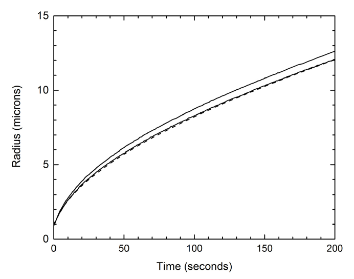
Figure 2: The dotted line shows the growth of a spherical crystal, calculated analytically as described in [25]. The two solid lines show the growth calculated with our numerical model using $N_{speed}=50$ (upper solid line) and $N_{speed}=200$ (lower solid line). The 2D model in $(r,z)$ was constrained to grow as a sphere for this test, as described in the text. This example demonstrates the excellent quantitative agreement between theory and our cellular automata model.

3.3 Crystal Growth

We include crystal growth by defining an accumulated mass parameter $M$ for each boundary pixel. We set $M=0$ when a pixel turns from an air pixel to a boundary pixel (as the crystal grows), and a boundary pixel turns into an ice pixel when $M$ reaches unity. Applying conservation of mass at the boundary yields [25]

$$\frac{dM}{dt}=\frac{c_{sat}}{c_{ice}}\frac{Dg}{\Delta\xi X_{0}^{2}}\sum\alpha\sigma f$$

where the sum is over all neighboring ice pixels that drain the boundary pixel. Here $\alpha$ and $\sigma$ are evaluated at the boundary pixel, $f=f_{\pm}$ for $r$ neighbors and $f=1$ for $z$ neighbors.

Following [13], we separate the relaxation of the $\sigma$ field from crystal growth. After relaxing the $\sigma$ field with the appropriate boundary conditions, we then calculate $dM/dt$ for all the boundary pixels. From this we advance the physical time by an amount $\Delta t$ such that $M\rightarrow 1$ for one, and only one, boundary pixel. This pixel is then converted to ice, the other boundary pixels have their respective $M$ increased by the appropriate amounts, and the $\sigma$ field is again relaxed before the next growth cycle. The relaxation step is essentially the same as the initial relaxation described above, but using $N_{speed}$ iterations. This is much smaller than the number of iterations used in the initial relaxation, because the perturbation of the $\sigma$ field is rather small when a single boundary pixel turns to ice.

Since our goal was to produce a numerical growth model for quantitative comparison with experimental data, we tested the model extensively using analytic results for the diffusion-limited growth of simple morphologies, as described in [25]. Figure 2, for example, shows our model reproduction of the growth of a spherical crystal. Because a spherical morphology is unstable to the Mullins-Sekerka growth instability, we maintained the spherical shape by slightly adjusting the accumulated mass parameter $M$ on the crystal boundary at each growth step, transferring mass between boundary pixels while conserving total mass in the process. Figure 2 demonstrates that our cellular automata model yields excellent quantitative agreement with the analytic solution. Note that reducing $N_{speed}$ results in an incomplete relaxation of the supersaturation field, and a corresponding increase in the crystal growth velocity.

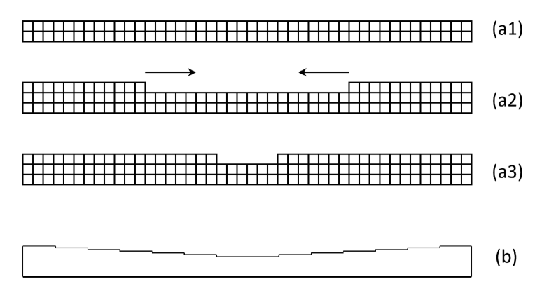
Figure 3: These sketches depict the growth of a basal facet atop a columnar ice crystal, in all cases showing a cross section of the facet in $(r,z)$ space, with $r=0$ at the center of the sketches. The top three sketches (a1-a3) show our model crystal. It begins as a perfectly faceted surface (a1), then a new terrace nucleates at the edge of the facet (a2), and the new terrace grows inward (a2-a3). The bottom sketch (b) shows our molecular picture of this same surface. New molecular terraces again nucleate at the facet edge and grow inward, but many molecular steps are present on the surface at all times. The coarse $z$ resolution of the cellular automata model limits our ability to model this slightly concave faceted surface.

3.4 Model Limitations

It is instructive at this point to consider the differences between our molecular picture of a growing faceted surface and the corresponding macroscopic cellular automata model, as shown in Figure 3. This depicts, for example, a basal facet atop a columnar ice crystal. When there are no available steps in the macroscopic model (a1), the growth is determined by the nucleation of new layers set by $\alpha_{facet}.$ But when a step appears, $\alpha$ increases substantially near the kink site. If $x_{s}$ is larger than $(La/\Delta z)$, where $L$ is the size of the model crystal, then $\alpha\rightarrow 1$ over the entire facet except on the top terrace. In this new state (a2), the step grows quite rapidly across the surface (a3), until it reaches the center of the facet and there are again no steps.

In the molecular picture shown by sketch (b) in Figure 3, the surface includes a large number of molecular steps, and these steps all grow simultaneously inward. The attachment coefficient is $\alpha\approx 1$ in a strip roughly $x_{s}$ wide next to each molecular step, and is $\alpha=\alpha_{facet}\ll 1$ otherwise. The overall growth velocity of the facet is set by the step separation $x_{step}$ together with the nucleation of new steps determined by $\alpha_{facet}.$ (Even this picture is too simple, as step bunching [27] will result in macrosteps on the ice surface, which are often seen in ice growth experiments.)

An important difference in these two pictures is that the real crystal contains multiple steps growing simultaneously, while the macroscopic model exhibits slow faceted growth (with a slow increase in the accumulated mass parameter) punctuated by the rapid completion of new terraces. In both cases, the overall growth velocity is determined by the generation of new terraces at the edge of the facet, and our model includes this key feature of ice growth. However the model provides only an imperfect representation of the growing faceted surface, as the model resolution $\Delta z$ is simply not sufficient to represent the large number of simultaneous terraces present on vicinal surfaces. Thus this model should work adequately in the limit of layer-by-layer growth, and again for surfaces that are sufficiently curved to include more than one $\Delta z$ step at all times. But vicinal angles in the range $a/L<\theta<\Delta z/L$ cannot be modeled with perfect fidelity. This shows that our inclusion of surface diffusion in the cellular automata formalism has improved our ability to model faceted growth, relative to a model with no surface diffusion. However, the coarse spatial resolution means that this model still cannot be expected to reproduce real crystal growth with perfect fidelity.

3.5 Forced Faceting

We found it useful to include an optional “forced faceting” feature in our model to partially address its deficiencies when dealing with nearly faceted surfaces. When this feature is turned on, we collect all the accumulated mass $dM$ on the top terrace at each growth step and transfer it to the nearest inner kink site. This action guarantees layer-by-layer growth while conserving mass in the process. The top terrace $dM$ values are not transferred when the top terrace extends to $r=0$ (for basal facets) or $z=0$ (for prism facets). This action assumes that new terraces nucleate at the outer edges of facets, which is true for our simple growth morphologies.

We often use this feature when an experimental growth morphology is perfectly faceted (to the resolution of our imaging) and the model produces only a partially faceted morphology. The difference may lie in our assumption of an infinite Ehrlich–Schwoebel barrier, since a leaky barrier will promote faceting. But the difference may also come from our imperfect modeling of nearly faceted surfaces, as described above. Our rationale for including this model feature will become somewhat clearer when examining a specific experimental case study.

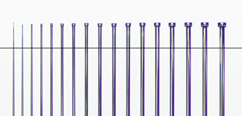
Figure 4: A composite image showing the growth of a faceted block on the end of a thin ice needle as a function of time. The ice crystal was grown in air at a temperature of -10 C, with a supersaturation of $\sigma_{\infty}\approx 11$ percent. The needle axis is along the crystal’s $c$ axis. The needle shrank slightly (first and second images) as the temperature equilibrated in the growth chamber, and grew thereafter. The total needle length was about two millimeters, and the needle base provided a stable reference point for measuring the axial growth. Scale for this image is provided by the measurements in Figure 5.

4 An Illustrative Example

As our primary goal is the quantitative analysis of ice growth data, it is instructive to examine some sample data in detail. Figure 4 shows a series of images of an ice needle as a function of time as it grew in the apparatus described in [31]. Analysis of these images yielded the needle radius $R_{needle}(t)$, block radius $R_{block}(t)$, and needle height $H(t)$ as a function of time, as shown in Figure 5. The radii were defined to give the same area as the hexagonal cross section of the corresponding needle or block, and the time axis in the plot was shifted to yield a (slightly extrapolated) straight needle at $t=0.$ The total needle length was measured relative to a fixed reference at the needle base (not shown in Figure 4), and $H(t)$ was shifted to give an arbitrary $H=24$ $\mu$m at $t=0.$

To model these data, we assume that the attachment coefficients on the facet surfaces have the form $\alpha_{facet}=A\exp(-\sigma_{0}/\sigma),$ as described in the previous section, and for nonfaceted sites we assume $\alpha=1.$After examining numerous models using a range of input parameters, we found that the needle radius $R_{needle}(t)$ was an especially good indicator of the supersaturation $\sigma_{\infty}$ far from the growing crystal. We found that $R_{needle}(t)$ was roughly proportional to $\sigma_{\infty}$, plus $R_{needle}(t)$ was rather insensitive to $\alpha_{basal}$ and $\alpha_{prism}.$ This behavior arises because the needle growth is largely diffusion limited, as can be seen from the analytic solution for the growth velocity $v=dR_{needle}/dt$ of an infinitely long needle [25], which gives

$$v=\frac{\alpha\alpha_{diffcyl}}{\alpha+\alpha_{diffcyl}}v_{kin}\sigma_{Rout}$$

where $\alpha=\alpha_{prism}$ is the attachment coefficient at the needle surface (which is a prism facet), $\sigma_{Rout}$ is the supersaturation at the outer boundary, and

$$\alpha_{diffcyl}=\frac{1}{B}\frac{X_{0}}{R_{needle}}$$

with $B=\log(R_{out}/R_{needle})$. With $R_{needle}=10$ $\mu$m and assuming $B\approx 8$, this gives $\alpha_{diffcyl}\approx 0.002,$ which is quite small. This means that $\alpha_{diffcyl}\ll\alpha_{prism}$ is a reasonable approximation, giving $v\approx\alpha_{diffcyl}v_{kin}\sigma_{Rout}$ independent of $\alpha_{prism}.$

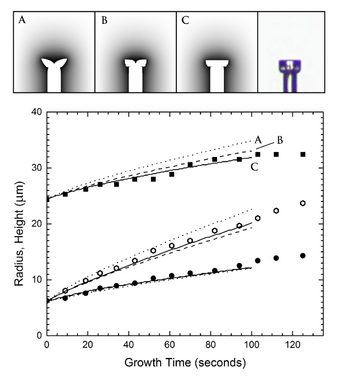
Figure 5: The data points show measurements of the images in Figure 4, giving the needle radius $R_{needle}(t)$ (at a position 200 $\mu$m below the needle tip) (solid round points), the block radius $R_{block}(t)$ (open round points) and the needle height $H(t)$ (solid square points) as a function of time. The $H(t)$ points were shifted to give $H(0)=24$ $\mu$m for plotting. The curves show models described in the text. The small images show corresponding model cross sections at $t=100$ seconds, along with the observed crystal at the same time and scale.

By running a series of models, we found that $\sigma_{\infty}\approx 2.5$ percent gave a good fit to $R_{needle}(t),$ a value that is considerably less than the experimental value of $\sigma_{\infty}\approx 11$ percent. This difference arises mainly because we typically use $R_{out}=72$ $\mu$m in our models, giving $B\approx 2.5.$ The experimental outer boundary is not precisely defined, but estimating $R_{out}=2$ cm gives $B\approx 8,$ and the ratio of these explains most of the difference in $\sigma_{\infty}.$

Given the various experimental and model uncertainties, we adjusted $\sigma_{\infty}$ at the outer boundary of our model space to best fit $R_{needle}(t),$ and we used $\sigma_{\infty}=2.5$ percent for all the models shown in Figure 5. Other model parameters that did not change from model to model are $Z_{out}=116$ $\mu$m, $T=-10$ C, $R_{needle}(t=0)=6.2$ $\mu$m, $H(t=0)=50$ $\mu$m, $\delta=0.3$ nm, $n_{SD}=10^{4},$ and $N_{speed}=50.$

Model A shown in Figure 5 used the parameters $M_{A}=\{\alpha_{basal}=[1,1],\alpha_{prism}=[1,0.7]\}$ and $A_{SD}=0$, where we have used the shorthand notation $\alpha=[A,100\sigma_{0}].$ Choosing $A_{SD}=0$ for both facets means that the model is essentially that described in [25], with no surface diffusion terms. Model B was the same as Model A, except that it used $A_{SD}=1$ on both facets. Model C was the same as Model B, expect that it also used forced faceting on the basal surface.

From this example we see that adding surface diffusion promotes faceting. Model A, with no surface diffusion, showed essentially no faceting, while Model B was closer to having faceted basal and prism surfaces. Still, Model B showed basal hollowing that was not seen in the experimental crystal. The growth velocities were changed only a small amount, owing to the fact that the growth was substantially diffusion limited.

5 Discussion

One clear conclusion from this investigation is that surface diffusion is likely an important factor in modeling ice crystal growth using cellular automata. Even if the diffusion length $x_{s}$ is smaller than the model resolution $\Delta z,$ the effects of surface diffusion can extend to rather large distances in the model, of order $n_{SD}=(x_{s}/a)$ pixels. This complicates cellular automata models, as surface diffusion is a nonlocal phenomenon. While the importance of surface diffusion follows from the fairly simple argument described above, it was not included in earlier cellular automata models of ice crystal growth.

We implemented what we believe is a fairly accurate approximation of surface diffusion by simply increasing $\alpha$ at surface points that are near kink sites, as prescribed above, ignoring mass transfer to the kink sites. This works because increasing the accumulated mass near kink sites has essentially the same effect on the overall growth behavior as transfering the accumulated mass to the relevant kink sites. Calcuating the necessary $\alpha_{SD}$ depends only on the crystal geometry at a given time, and does not require much additional computation time.

When ice crystals are grown in air near one bar, which is a common experimental condition, faceted surfaces are generally not faceted at the molecular level, but are slightly concave. New layers nucleate at the facet edges, where the supersaturation is highest, and terraces grow inward from the edges. In many realistic circumstances, this means that $\alpha\approx 1$ at essentially all points on the crystal surface, except for the top terraces, where $\alpha=\alpha_{facet}.$ Moreover the top terraces might be exceedingly narrow for typical facets – a facet with a 1 $\mu$m depression over a 100 $\mu$m width means that the top terraces are only 100 molecules wide. This makes for a somewhat remarkable circumstance – apparently quite common in ice growth from vapor – where $\alpha\approx 1$ everywhere on a complex faceted ice crystal except for a few extremely narrow terraces where $\alpha\approx\alpha_{facet}\ll 1.$

Another conclusion from this investigation is that accurately determining the intrinsic $\alpha_{facet}(\sigma,T)$ for faceted ice surfaces is extremely challenging when using only growth measurements made in air. The effects of bulk diffusion together with surface diffusion are subtle and difficult to model accurately, making it impractical in many circumstances to extract $\alpha_{facet}(\sigma,T)$ with any real accuracy. Fortunately, observing growth in near vacuum seems to alleviate these problems sufficiently to allow accurate measurements of $\alpha_{facet}(\sigma,T)$ [30]. Assuming that the $\alpha_{facet}(\sigma,T)$ values determined at pressures near $0.01$ bar apply to pressures near 1 bar, these $\alpha_{facet}(\sigma,T)$ can then be used as input to the numerical models to further investigate structure formation that arises during diffusion-limited growth at higher pressures.

References

- [1] R. Trivedi and W. Kurz. Dendritic growth. Inter. Mater. Rev., 39:49–74, 1994.
- [2] E. A. Brener. Three-dimensional dendritic growth. J. Cryst. Growth, 166:339–346, 1996.
- [3] I. Avramov. Kinetics of growth of nanowhiskers (nanowires and nanotubes). Nanoscale Res. Lett., 2:235–239, 2007.
- [4] H. Zhang and et al. Aligned two- and three-dimensional structures by directional freezing of polymers and nanoparticles. Nature Mater., 4:787–793, 2005.
- [5] M. C. Cross and P. C. Hohenburg. Pattern formation outside of equilibrium. Rev. Mod. Phys., 65:851–1112, 1993.
- [6] K. Kassner. Pattern formation in diffusion-limited crystal growth. World Scientific Publishing, 1996.
- [7] K. G. Libbrecht. The physics of snow crystals. Rep. Prog. Phys., 68:855–895, 2005.
- [8] J. Nelson. Growth mechanisms to explain the primary and secondary habits of snow crystals. Phil. Mag., 81:2337–2373, 2001.
- [9] H. R. Pruppacher and J. D. Klett. Microphysics of Clouds and Precipitation. Kluwer Academic Publishers, 1997.
- [10] C. A. Reiter. A local cellular model for snow crystal growth. Chaos, Solitons, and Fractals, 23:1111–1119, 2005.
- [11] Janko Gravner and David Griffeath. Modeling snow-crystal growth: A three-dimensional mesoscopic approach. Phys. Rev. E, 79:011601, Jan 2009.
- [12] John W. Barrett, Harald Garcke, and Robert Nürnberg. Numerical computations of faceted pattern formation in snow crystal growth. Phys. Rev. E, 86:011604, Jul 2012.
- [13] James G. Kelly and Everett C. Boyer. Physical improvements to a mesoscopic cellular automaton model for three-dimensional snow crystal growth. arXiv:, (1308.4910), 2013.
- [14] S. Y. Hong, J. Dudhia, and S. H. Chen. A revised approach to ice microphysical processes for the bulk parameterization of clouds and precipitation. Mon. Weath. Rev., 132:103–120, 2004.
- [15] M. Matsumoto, S. Saito, and I. Ohmine. Molecular dynamics simulation of the ice nucleation and growth process leading to water freezing. Nature, 416:409–413, 2002.
- [16] J. G. Dash, A. W. Rempel, and J. S. Wettlaufer. The physics of premelted ice and its geophysical consequences. Rev. Mod. Phys., 78:695–741, 2006.
- [17] A. Karma and W. J. Rappel. Phase-field method for computationally efficient modeling of solidification with arbitrary interface kinetics. Phys. Rev. E, 53:R3017–R3020, 2006.
- [18] I. Singer-Loginova and H. M. Singer. The phase field technique for modeling multiphase materials. Rep. Prog. Phys., 71:106501, 2008.
- [19] A. Schmidt. Computation of three dimensional dendrites with finite elements. J. Comp. Phys., 125:293–312, 1996.
- [20] Etsuro Yokoyama. Formation of patterns during growth of snow crystals. J. Cryst. Growth, 128:251–257, 1993.
- [21] Stephen E. Wood and Marcia B. Baker. New model for vapor growth of hexagonal ice crystals in the atmosphere. J. Geophys. Res., 106:4845–4870, 2001.
- [22] Janko Gravner and David Griffeath. Modeling snow crystal growth i: Rigorous results for packard’s digital snowflakes. Expt. Math., 15:421–444, 2006.
- [23] Janko Gravner and David Griffeath. Modeling snow crystal growth ii: A mesoscopic lattice map with plausible dynamics. Physica D, 237:385–404, 2008.
- [24] Kenneth G. Libbrecht. Physically derived rules for simulating faceted crystal growth using cellular automata. arXiv:, (0807.2616), 2008.
- [25] Kenneth G. Libbrecht. Quantitative modeling of faceted ice crystal growth from water vapor using cellular automata. J. Computational Methods in Phys., (ID-174806), 2013.
- [26] K. G. Libbrecht. On the equilibrium shape of an ice crystal. arXiv:, (1205.1452), 2012.
- [27] Y. Saito. Statistical Physics of Crystal Growth. World Scientific Books, 1996.
- [28] H. Asakawa, G. Sazaki, and et al. Roles of surface/volume diffusion in the growth kinetics of elementary spiral steps on ice basal facets grown from water vapor. Cryst. Growth and Design, (14):3210–3220, 2014.
- [29] Kenneth G. Libbrecht. The surface diffusion length of water molecules on faceted ice: A reanalysis of ‘roles of surface/volume diffusion in the growth kinetics of elementary spiral steps on ice basal faces grown from water vapor’, by asakawa et al. arXiv:, (1509.06609), 2015.
- [30] Kenneth G. Libbrecht and Mark E. Rickerby. Measurements of surface attachment kinetics for faceted ice crystal growth. J. Crystal Growth, (377):1–8, 2013.
- [31] Kenneth G. Libbrecht. A dual diffusion chamber for observing ice crystal growth on c-axis ice needles. arXiv:, (1405.1053), 2014.