MPC on manifolds with an application to the control of spacecraft attitude on $\textrm{SO}(3)$

Abstract

We develop a model predictive control (MPC) design for systems with discrete-time dynamics evolving on smooth manifolds. We show that the properties of conventional MPC for dynamics evolving on $\mathbb{R}^{n}$ are preserved and we develop a design procedure for achieving similar properties. We also demonstrate that for discrete-time dynamics on manifolds with Euler characteristic not equal to 1, there do not exist globally stabilizing, continuous control laws. The MPC law is able to achieve global asymptotic stability on these manifolds, because the MPC law may be discontinuous. We apply the method to spacecraft attitude control, where the spacecraft attitude evolves on the Lie group $\text{SO}(3)$ and for which a continuous globally stabilizing control law does not exist. In this case, the MPC law is discontinuous and achieves global stability.

1 Introduction

Conventional model predictive control (MPC) [2] is developed for and usually applied to systems whose discrete-time dynamics evolve on the “flat” normed vector space $\mathbb{R}^{n}$. However, the configuration spaces of some systems are smooth manifolds that are not diffeomorphic to $\mathbb{R}^{n}$. To design the prediction dynamics for such systems, finite-dimensional manifolds may be embedded in $\mathbb{R}^{n}$, and standard integration schemes employed to derive the discrete-time update equation, enforcing their evolution on the manifold through the use of equality constraints. However, standard integration techniques do not preserve symmetries for systems evolving on manifolds, and this results in the integration not correctly representing the actual dynamics. Because of this, specific methods for integrating system dynamics that evolve on manifolds have been developed in, for example, [3, 4, 5].

As a motivating example, consider the attitude dynamics of a rigid body evolving on the manifold $\textrm{SO}(3)$. This manifold is a $3$-dimensional space which can be embedded in $\mathbb{R}^{n}$ for $n\geq 5$ but is not diffeomorphic to $\mathbb{R}^{n}$ for any $n$. The group $\textrm{SO}(3)$ is a particular case of a compact Lie group; for mechanical systems whose configuration space is a compact Lie group, the Lie group variational integrator (LGVI) [6] has been developed to obtain discrete-time update equations that preserve the underlying group structure. Unlike ordinary integration schemes, the LGVI also preserves the conserved quantities of motion [7] and is therefore a more realistic prediction model. Also unlike ordinary integration schemes, the LGVI equations of motion are significantly different from conventionally used, discrete-time dynamics. For instance, the LGVI for spacecraft attitude gives an equation of the form [8],

$$g_{k+1} =g_{k}f_{k},$$ (1a)

$$f_{k+1}J-Jf_{k+1}^{\text{T}} =Jf_{k}-f_{k}^{\text{T}}J+{h^{2}}u_{k},$$ (1b)

where $g_{k}\in\textrm{SO}(3)$ is the orientation, $f_{k}\in\textrm{SO}(3)$ is the change in $g_{k}$, $u_{k}$ is related to the external torques, $h$ is the length of the integration step. Indeed, (1b) is an implicit equation, and implicit equations are seldom used in conventional MPC prediction models.

The control of dynamics evolving on manifolds present additional challenges. On manifolds with Euler characteristic not equal to 1, there exist topological obstructions that imply the non-existence of globally-stabilizing, continuous control laws. This has been shown for the continuous-time setting [9], and is a consequence of the Poincaré-Hopf theorem [10]. In this paper, we appeal to the Lefschetz-Hopf theorem and derive a similar result for discrete-time dynamics.

In this paper we investigate the design of MPC for systems evolving in manifolds, with the aim of retaining properties of conventional MPC applied to flat spaces. The applications of MPC to systems whose dynamics evolve on manifolds have scarcely been considered, with the exceptions of [11, 12], which focus on computational issues, and have limited analysis of closed-loop properties.

In this paper, we first show that MPC on smooth manifolds achieves the same properties of conventional MPC in $\mathbb{R}^{n}$, namely, recursive feasibility and asymptotic stability of the equilibrium. Then we describe the design of the MPC terminal cost and terminal set that achieves such properties.

As an additional contribution of this paper, we show that when the manifold is compact, our MPC is able to achieve global closed-loop asymptotic stability in the state-unconstrained case. In particular, this property holds for manifolds with Euler characteristic not equal to 1, for which a continuous, globally stabilizing control law does not exist. Because MPC can produce discontinuous control laws [13], the topological obstruction for such manifolds is not restrictive in this case. Thus this paper highlights the capability to design possibly discontinuous, stabilizing feedback control laws with global stability properties, by employing a systematic and unified design procedure in the MPC framework.

A practical contribution of this paper is the presentation of a control law for the constrained control of spacecraft attitude, in which we apply our MPC scheme to the LGVI dynamics evolving on $\textrm{SO}(3)$.

The paper is organized as follows. Section 2 develops the MPC scheme and the conditions for closed-loop stability. Section 3 describes the design of the terminal penalty and terminal set constraint achieving closed-loop stability by exploiting a specifically designed local control law. Section 4 proves the non-existence of a globally stabilizing, continuous control law under certain assumptions, and hence the discontinuity of the MPC law. Section 5 presents simulation results for dynamics evolving on the Lie group $\textrm{SO}(3)$ and Section 6 summarizes the conclusions.

1.1 Notation

The notation is standard with a few notable exceptions. The set $\mathbb{Z}_{N}$ denotes the set of the first $N$ nonnegative integers and $\mathbb{Z}_{+}$ denotes the set of all nonnegative integers. For a set $\mathcal{A}$, its interior is denoted by $\operatorname{int}\mathcal{A}$, its closure by $\operatorname{cl}\mathcal{A}$, and its boundary by $\operatorname{bd}\mathcal{A}$. The set $\mathcal{A}^{N}$ represents $N$ copies of $\mathcal{A}$. The identity matrix is denoted $I_{n}\in\mathbb{R}^{n\times n}$ and an $n$-by-$m$ zero matrix is denoted $0_{n\times m}\in\mathbb{R}^{n\times m}$. For two functions $f,g:\mathbb{R}\rightarrow\mathbb{R}$, $f\circ g$ is their composition, and $g(t)=o(f(t))$ implies that $\lim_{t\rightarrow\infty}g(t)/f(t)=0$. A function $\alpha:[0,a)\rightarrow[0,\infty)$ is said to be class $\mathcal{K}$ if it is strictly increasing and $\alpha(0)=0$; furthermore $\alpha$ is said to be class $\mathcal{K}_{\infty}$ if $a=\infty$ and $\alpha(x)\rightarrow\infty$ as $x\rightarrow\infty$. Finally, for a sequence $\{v_{k},v_{k+1},\dots,v_{k+N}\}$, its predicted value at time $k$ is denoted by $\{v_{k|k},v_{k+1|k},\dots,v_{k+N|k}\}$.

2 MPC on manifolds

We begin by developing a general MPC law for application to smooth manifolds. In the construction of the control law, we follow ideas inspired by conventional nonlinear MPC laws [2], for systems whose dynamics evolve on $\mathbb{R}^{n}$. For instance, in order to ensure recursive feasibility of the finite horizon optimal control problem and to enlarge the domain of attraction, we utilize a terminal set and terminal cost function [2]. We thereby obtain a result on system stability that rigorously generalizes MPC stability results to a more generous class of systems whose dynamics evolve on manifolds. In this setting, we obtain a remarkable result that when the manifold is compact and there are no state constraints, this MPC law may provide global asymptotic stability.

Let $M$ be an $n$-dimensional smooth manifold, which is endowed with a metric $d$, and let $U$ be a compact subset of an $m$-dimensional smooth manifold. Note that the fact that all smooth manifolds are metrizable follows from Whitney’s embedding theorem [10]. Furthermore, all smooth manifolds admit a Riemannian metric [14]. Consider the dynamic update equation,

$$x_{k+1}=f(x_{k},u_{k}),$$ (2a)

$$f:M\times U\rightarrow M,$$ (2b)

where $x_{k}\in M$ and $u_{k}\in U$. The evolution on manifold is highlighted by using $M$ in the domain and co-domain of (2b); the function $f$ is continuously differentiable and satisfies $f(x_{e},u_{e})=x_{e}$ for some $x_{e}\in M$, which we refer to as the equilibrium of $f$, and some $u_{e}\in U$.

The system is subject to state and control constraints,

$$x_{k}\in\mathcal{X},~{}u_{k}\in\mathcal{U},$$ (3)

where $\mathcal{X}$ and $\mathcal{U}$ are compact and connected subsets of $M$ and $U$, respectively, that satisfy $x_{e}\in\operatorname{int}\mathcal{X}$ and $u_{e}\in\operatorname{int}\mathcal{U}$.

We introduce a cost function $\mathcal{V}_{N}:M\times U^{N}\rightarrow\mathbb{R}$ satisfying,

$$\mathcal{V}_{N}\left(x_{k};\{u_{k+i|k}\}_{i\in\mathbb{Z}_{N}}\right)\\ =F(x_{k+N|k})+\sum_{i\in\mathbb{Z}_{N}}L(x_{k+i|k},u_{k+i|k}),$$ (4)

where $x_{k+i+1|k}=f(x_{k+i|k},u_{k+i|k})$ is the predicted state at time $k+i+1$ for $i\in\mathbb{Z}_{N}$. The functions $L:M\times U\rightarrow\mathbb{R}$ and $F:M\rightarrow\mathbb{R}$ are twice continuously differentiable and have the following properties,

$$L(x_{e},u_{e})=F(x_{e})=0,$$ (5a)

$$L(x_{k},u_{k})\geq L(x_{k},u_{e})\geq\gamma(d(x_{k},x_{e})),$$ (5b)

$$F(x_{k})\geq\alpha(d(x_{k},x_{e})),$$ (5c)

for all $x_{k}\in M$ and $u_{k}\in U$, where $\gamma$ is a class $\mathcal{K}_{\infty}$, $\alpha$ is a class $\mathcal{K}$ function.

We now introduce the target set and terminal feedback law. These are required in order to enforce recursive feasibility, ensuring that if the state at the end of the prediction horizon is in the target set, it and the associated feedback control satisfy all constraints and are therefore feasible solutions to the finite horizon optimal control problem. Specifically, we introduce the target set $\mathcal{X}_{T}\subset\mathcal{X}$, which is compact and contains $x_{e}$ in its interior. We also introduce a control law $\kappa:M\rightarrow U$, which we refer to as the local control law satisfying,

$$\kappa(x_{k}) \in\mathcal{U},$$ (6a)

$$f(x_{k},\kappa(x_{k})) \in\mathcal{X}_{T},$$ (6b)

$$F(f(x_{k},\kappa(x_{k})))-F(x_{k}) \leq-L(x_{k},\kappa(x_{k})),$$ (6c)

for all $x_{k}\in\mathcal{X}_{T}$.

The MPC control law is obtained through the solution to the following problem,

$$\min_{\{u_{k+i|k}\}_{i\in\mathbb{Z}_{N}}}~{} \mathcal{V}_{N}\left(x_{k};\{u_{k+i|k}\}_{i\in\mathbb{Z}_{N}}\right),$$ (7a)

$$\operatorname{subject~{}to}~{} x_{k+i+1|k}=f(x_{k+i|k},u_{k+i|k}),$$ (7b)

$$x_{k+i|k}\in\mathcal{X},$$ (7c)

$$u_{k+i|k}\in\mathcal{U},~{}\forall i\in\mathbb{Z}_{N},$$ (7d)

$$x_{k+N|k}\in\mathcal{X}_{T}.$$ (7e)

When the solution to (7) exists, it is denoted by $\mathcal{V}_{N}^{*}(x_{k})$ and the control sequence solving it is denoted by $\{u_{k+i|k}^{*}\}_{i\in\mathbb{Z}_{N}}$.

The input obtained from the model predictive control law at time $k$ is the first element in the sequence solving (7),

$$u_{k}=u_{k|k}^{*}.$$ (8)

The MPC law defined above can be used on differentiable manifolds. We will now show that the domain of attraction of the equilibrium $x_{e}$ of the closed-loop system defined by (2) and (8) coincides with the set of initial conditions that can be steered using open-loop control to the target set without violating the constraints. Define,

$$\mathcal{D}_{N}=\{x_{k}\in M:\exists\{u_{k+i|k}\}_{i\in\mathbb{Z}_{N}}\in\mathcal{U}\\ \textrm{ s.t.~{}(\ref{equ:mpcopt_1})-(\ref{equ:mpcopt_3}) are satisfied}\}.$$ (9)

We state the main result below and provide the proof in the appendix.

Theorem 1

Let $x_{0}\in\mathcal{D}_{N}$. Then (i) the finite horizon optimal control problem (7) is feasible for all $k\in\mathbb{Z}_{+}$ and (ii) $x_{e}\in M$ is the asymptotically stable equilibrium for closed-loop system defined by (2) and (8) with a basin of attraction $\mathcal{D}_{N}$, i.e., for any $x_{0}\in\mathcal{D}_{N}$ and $\varepsilon>0$, there exists $\delta>0$ such that $d(x_{0},x_{e})<\delta$ implies that $d(x_{k},x_{e})<\varepsilon$ for all $k>0$, and furthermore, $d(x_{k},x_{e})\rightarrow 0$ as $k\rightarrow\infty$.

Note that whenever $\mathcal{D}_{N}=M$, Theorem 1 implies that the control law (8) is globally stabilizing. In general, this may not be possible because $\mathcal{D}_{N}$ is a subset of $\mathcal{X}$ and $\mathcal{X}$ is a subset of $M$. However, if $M$ is a compact manifold, then $\mathcal{X}$ may be equal to $M$; in this case, a large enough $N$ can be chosen so that $\mathcal{D}_{N}=\mathcal{X}$. Therefore, based on the following proposition, it is possible to guarantee global asymptotic stability in the case where $M$ is compact.

Proposition 2

Suppose $M$ is compact and let $\mathcal{D}_{\infty}$ be the set of initial conditions $x_{0}$ such that there exists a sequence of control inputs steering $x_{0}$ to $x_{e}$,

$$\mathcal{D}_{\infty}=\{x_{k}\in M:\exists\{u_{k+i|k}\}_{i\in\mathbb{Z}_{+}}\in\mathcal{U},\\ \lim_{k\rightarrow\infty}x_{k+i|k}=x_{e}\}.$$ (10)

Suppose the system (2) is state-unconstrained so that $\mathcal{X}=M$ and suppose $\mathcal{D}_{\infty}=M$. Then there exists a finite $N^{*}$ such that $\mathcal{D}_{N^{*}}=M$ and therefore the closed-loop system defined by (2) and (8) is globally asymptotically stable.

Proof. It is clear that for any finite $N\geq 0$, $\mathcal{D}_{N}\subset\mathcal{D}_{\infty}=M$ and that the set $\operatorname{cl}(M\setminus\mathcal{X}_{T})=\operatorname{cl}(\mathcal{D}_{\infty}\setminus\mathcal{X}_{T})$ is a subset of $\mathcal{D}_{\infty}$. Let $N(x)=\inf\{i:x_{k}=x,~{}\exists\{u_{k+i|k}\}_{i\in\mathbb{Z}_{+}}\in\mathcal{U},~{}x_{k+i|k}\in\mathcal{X}_{T}\}$ be the minimum number of control steps required to guide an initial condition $x\in D_{\infty}=M$ to the set $\mathcal{X}_{T}$. According to the definition of $\mathcal{D}_{\infty}$ and the fact that $x_{e}\in\operatorname{int}\mathcal{X}_{T}$, $N(x)$ is finite for all $x\in\operatorname{cl}(M\setminus\mathcal{X}_{T})$. Let $N^{*}=\sup\{N(x):x\in\operatorname{cl}(M\setminus\mathcal{X}_{T})\}$. Since $\operatorname{cl}(M\setminus\mathcal{X}_{T})$ is compact, $N^{*}$ is finite.

Let $x\in M$. Therefore there exists a control sequence $\{u_{k+i|k}\}_{k\in\mathbb{Z}_{+}}$ guiding $x_{k}=x$ to $x_{e}$ and $x_{k+N^{*}|k}\in\mathcal{X}_{T}$. The sequence $\{u_{k+i|k}\}_{k\in\mathbb{Z}_{N^{*}}}$ is feasible for (7) because it satisfies both state and control constraints. Therefore, $\mathcal{D}_{N^{*}}\supset\mathcal{D}_{\infty}=M$.

By Theorem 1, $M$ is the domain of attraction of the closed-loop system defined by (2) and (8), and therefore the closed-loop system is globally asymptotically stable at $x_{e}$.

3 Local control law

The development of the control law (8) depends on the design of target set $\mathcal{X}_{T}$ and the local control law $\kappa:M\rightarrow U$ with the properties enumerated in (6). In this section, we describe a procedure to construct $\mathcal{X}_{T}$ and $\kappa$ that satisfy the properties in (6) for dynamics (2) evolving on manifolds. For conventional MPC, the terminal set and terminal cost are designed from a linearization of the dynamics around the equilibrium [2]. In our approach, we utilize diffeomorphisms to obtain local coordinates, on which we construct a stabilizing controller; we then transform the local control law to the coordinates of the original system.

To begin, because $M$ is an $n$-dimensional manifold and $U$ is a compact subset of an $m$-dimensional manifold that contains $u_{e}$ in its interior, there exist local diffeomorphisms at $x_{e}$ and $u_{e}$ [15, 10],

$$\phi:V\rightarrow M,\psi:W\rightarrow U,$$ (11)

where $V\subset\mathbb{R}^{n}$ and $W\subset\mathbb{R}^{m}$ are open neighborhoods of $x_{e}$ and $u_{e}$, respectively. Furthermore, because the equilibrium is in the interior of both $V$ and $W$, $f$ is continuously differentiable, and $f(x_{e},u_{e})=x_{e}$, there exists an open neighborhood $V^{\prime}\times W^{\prime}\subset V\times W$ of $(0,0)$ such that $f(\phi(V^{\prime})\times\psi(W^{\prime}))\subset\phi(V)$. Therefore,

$$f^{\prime}=\phi^{-1}\circ f\circ(\phi\times\psi),$$ (12)

and the derivative of $f^{\prime}$ at $(0,0)$ is,

$$df^{\prime}_{(0,0)}=d\phi_{0}^{-1}\circ df_{(x_{e},u_{e})}\circ(d\phi_{0}\times d\psi_{0}).$$ (13)

Let $\xi_{k}\in\mathbb{R}^{n}$ and $\eta_{k}\in\mathbb{R}^{m}$ and let $A=df^{\prime}_{(0,0)}\circ(I_{n},0_{m\times n})$ and $B=df^{\prime}_{(0,0)}\circ(0_{n\times m},I_{m})$. Define a linear update equation,

$$\xi_{k+1}=A\xi_{k}+B\eta_{k}.$$ (14)

Let,

$$L^{\prime}=\frac{1}{\lambda}L\circ(\phi\times\psi),$$ (15)

where $0<\lambda<1$ is a scalar parameter. Consider the discrete-time algebraic Riccati equation,

$$0=A^{\textrm{T}}PA-P+Q$$ (16)

$$-(A^{\textrm{T}}PB+N)(BPB^{\textrm{T}}+R)^{-1}(A^{\textrm{T}}PB+N)^{\textrm{T}},$$

where,

$$\begin{bmatrix}Q&N\\ N^{\textrm{T}}&R\end{bmatrix}=\operatorname{Hess}L^{\prime}(0,0).$$ (17)

is the Hessian of $L^{\prime}$ at $(0,0)$. A positive-definite solution $P$ to the algebraic Riccati equation (16) exists if and only if the pair $(A,B)$ is stabilizable and the associated symplectic pencil does not have eigenvalues on the unit circle [16]. A sufficient condition implying the latter is that $\operatorname{Hess}L^{\prime}(0,0)$ is positive-definite.

Suppose a positive-definite solution $P$ exists for (16). Let $\kappa^{\prime}:\mathbb{R}^{n}\rightarrow\mathbb{R}^{m}$ be a stabilizing feedback control law for (14) where,

$$\kappa^{\prime}(\xi_{k})=-(BPB^{\textrm{T}}+R)^{-1}(A^{\textrm{T}}PB+N)^{\textrm{T}}\xi_{k}.$$ (18)

We introduce a set $\mathcal{P}_{c}\subset\mathbb{R}^{n}$ and a function $F^{\prime}:\mathbb{R}^{n}\rightarrow\mathbb{R}$ where,

$$\mathcal{P}_{c} =\{\xi\in\mathbb{R}^{n}:F^{\prime}(\xi)\leq c\},$$ (19)

$$F^{\prime}(\xi) =\xi^{\textrm{T}}P\xi.$$ (20)

Because $P$ is the solution to the algebraic Riccati equation (16), the design of the control law (18) implies that the set $\mathcal{P}_{c}$ is compact and invariant with respect to the closed loop dynamics (14), (18).

Our goal is to use $\mathcal{P}_{c}$ and $\kappa^{\prime}$ in order to design the target set $\mathcal{X}_{T}$ and local control law $\kappa$. The following result is a proof of the existence of $\mathcal{X}_{T}$ and $\kappa$.

Proposition 3

Let $F=F^{\prime}\circ\phi^{-1}$. Suppose there exists a solution $P>0$ to the algebraic Riccati equation (16). Then there exists $c>0$ such that the set $\mathcal{X}_{T}\subset\phi(\mathcal{P}_{c})$ and control law $\kappa=\kappa^{\prime}\circ\phi^{-1}$ satisfy the assumptions of (6).

Proof. Firstly, we show that $F$ satisfies the assumptions made in the design of the MPC law. Because $M$ is a smooth manifold, $\phi$ is smooth and this, along with the smoothness of $F^{\prime}$, implies that $F$ is smooth. Furthermore, $F(x_{e})=F^{\prime}(\phi^{-1}(x_{e}))=F^{\prime}(0)=0$ which satisfies (5a). Finally, due to the equivalence of norms on $\mathbb{R}^{n}$ and (5b), there exists $r>0$ such that $F(x)=F^{\prime}(\phi^{-1}(x))=\phi^{-1}(x)^{\textrm{T}}P\phi^{-1}(x)\geq r\phi^{-1}(x)^{\textrm{T}}Q\phi^{-1}(x)=rL^{\prime}(\phi^{-1}(x),0)=rL(x,u_{e})\geq r\cdot\gamma(d(x,x_{e}))$. Since $r\cdot\gamma$ is a class $\mathcal{K}$ function, (5c) is satisfied.

If $c>0$, then by definition (19), the set $\mathcal{P}_{c}$ has a non-empty interior, which contains the origin. Because $V^{\prime}$ contains the origin, there exists $c^{\prime}>0$ such that $\mathcal{P}_{c^{\prime}}\subset V^{\prime}$ and $\kappa^{\prime}(\mathcal{P}_{c^{\prime}})\subset U^{\prime}$ and therefore $\phi(\mathcal{P}_{c^{\prime}})=\{x:F(x)\leq c^{\prime}\}$ because $F^{\prime}(\phi^{-1}(x))=F(x)$.

Furthermore, because $(x_{e},u_{e})$ is in the interior of $\mathcal{X}\times\mathcal{U}$ and $\kappa^{\prime}$ is $C^{1}$, there exists $c^{\prime\prime}>0$ such that $(\phi(\xi),\kappa(\phi(\xi)))\in\mathcal{X}\times\mathcal{U}$ for all $\xi\in\mathcal{P}_{c^{\prime\prime}}$. It remains to show that there exists a $c>0$ such that $\mathcal{X}_{T}=\phi(\mathcal{P}_{c})$ satisfies conditions (6b) and (6c).

Note that,

$$f^{\prime}(\xi_{k},\eta_{k}) =A\xi_{k}+B\eta_{k}+o(\|(\xi_{k},\eta_{k})\|),$$

$$L^{\prime}(\xi_{k},\eta_{k}) =\begin{bmatrix}\xi_{k}^{\textrm{T}}&\eta_{k}^{\textrm{T}}\end{bmatrix}\begin{bmatrix}Q&N\\ N^{\textrm{T}}&R\end{bmatrix}\begin{bmatrix}\xi_{k}\\ \eta_{k}\end{bmatrix}$$

$$\hskip 72.26999pt+o(\|(\xi_{k},\eta_{k})\|^{2}),$$

$$F^{\prime}(\xi_{k}) =\xi_{k}^{\textrm{T}}P\xi_{k}.$$

Therefore, $F^{\prime}(\xi_{k+1})-F^{\prime}(\xi_{k})+L^{\prime}(\xi_{k},\kappa^{\prime}(\xi_{k}))=F^{\prime}\circ f^{\prime}(\xi_{k},\kappa^{\prime}(\xi_{k}))-F^{\prime}(\xi_{k})+L^{\prime}(\xi_{k},\kappa^{\prime}(\xi_{k}))=o(\|\xi_{k}\|^{2})$. This implies that for $x_{k}\in\mathcal{P}_{c^{\prime}}$, $F(x_{k+1})-F(x_{k})+L(x_{k},\kappa(x_{k}))=F\circ f(x_{k},\kappa(x_{k}))-F(x_{k})+L(x_{k},\kappa(x_{k}))=F^{\prime}\circ f^{\prime}(\phi^{-1}(x_{k}),\kappa(\phi^{-1}(x_{k})))-F^{\prime}(\phi^{-1}(x_{k}))+\lambda L^{\prime}(\phi^{-1}(x_{k}),\kappa(\phi^{-1}(x_{k})))+o(\|\phi^{-1}(x_{k})\|^{2})$, and therefore,

$$F(x_{k+1})-F(x_{k})+L(x_{k},\kappa(x_{k}))$$

$$~{}=-(1-\lambda)L^{\prime}(\phi^{-1}(x_{k}),\kappa(\phi^{-1}(x_{k})))+o(\|x_{k}\|^{2}).$$

Because $L^{\prime}$ is positive definite, for any choice of $0<\lambda<1$, there exists $c^{\prime\prime\prime}\geq 0$ such that (6b) and (6c) are satisfied. Let $c=\min(c^{\prime\prime},c^{\prime\prime\prime})$ to complete the proof.

4 Globally stabilizing control law

The results of Section 2 show that the MPC law (8) is globally asymptotically stabilizing under certain assumptions. We will now show that this implies that the control law generated by MPC is necessarily discontinuous for certain classes of manifolds. Specifically, we will show that there does not exist a globally stabilizing, continuously differentiable control law for compact manifolds $M$ with Euler characteristic $\chi(M)$ not equal to 1. The Euler characteristic is a topological invariant that restricts the possible combinations of sinks and sources that can exist for a continuous vector field defined on the manifold [10]. Generally, only a manifold with Euler characteristic of 1 admits a continuous vector field with one sole sink and no other equilibrium. As an example, the normed vector space $\mathbb{R}^{n}$ has an Euler characteristic of 1, the sphere $S^{2}$ has an Euler characteristic of 2, and all compact Lie groups have an Euler characteristic of 0. Therefore, the sphere and compact Lie groups do not admit continuous vector fields with one sink and no other equilibrium.

We begin by noting that there exists no globally stabilizing, continuously differentiable, continuous-time control law on compact manifolds $M$ [9]. The proof of the continuous-time result appeals to a consequence of the Poincaré-Hopf theorem, which states that the sum of fixed point indexes on $M$ must be equal to the Euler characteristic. Since the index of a sink is equal to 1, if $\chi(M)\neq 1$, the set of fixed points on $M$ cannot consist of solely a sink. In discrete-time, the analogous result to the Poincaré-Hopf theorem is the Lefschetz-Hopf theorem, of which we use a strong version below.

Theorem 4 (Lefschetz-Hopf [17])

Let $M$ be a compact smooth manifold and let $f_{0}:M\rightarrow M$ be a continuous map that is homotopic to the identity map $\textrm{id}:M\rightarrow M$. Suppose the set of points $x\in M$ satisfying $x=f_{0}(x)$ is finite. Then,

$$\sum_{x_{0}\in\{x:x=f_{0}(x)\}}i_{f_{0}}(x_{0})=\chi(M),$$ (21)

where $i_{f_{0}}(x_{0})$ is the fixed point index of $f_{0}$ at $x_{0}$.

The fixed point index is a property characterizing an equilibrium. Note that when the fixed point is an asymptotically stable equilibrium, i.e., a sink, then its fixed point index is equal to 1. This fact is used in the proof of the discrete-time analogue to Brockett’s necessary condition [18] for systems where $M=\mathbb{R}^{n}$ but, to the authors’ knowledge, an equivalent result for $M$ with $\chi(M)\neq 1$ does not appear elsewhere in the literature. Hence we present below a theorem proving that there exists no globally-stabilizing, continuous, discrete-time control law on manifolds $M$ with $\chi(M)\neq 1$ whenever the closed-loop dynamics are homotopic to the identity.

Theorem 5

Let $M$ be a compact smooth manifold. Consider the dynamics (2) and assume the unforced dynamics map $f_{0}:x\mapsto f(x,u_{e})$ is homotopic to identity. Further assume that there exists a control law $u_{k}=\kappa(x_{k})$ with globally asymptotically stable equilibrium $x=x_{e}$, and define the resulting closed-loop dynamics by $x_{k+1}=f_{1}(x_{k})=f(x_{k},\kappa(x_{k}))$. If $\chi(M)\neq 1$, then $\kappa:M\rightarrow U$ is not continuous.

Remark 1

The homotopy assumption is crucial since it ensures that the unforced dynamics correspond to a continuous deformation of the system from an equilibrium configuration. A case where this assumption is violated is when the unforced map satisfies $f_{0}(x_{k})=x_{e}$ for all $x_{k}\in M$. In this case, $\kappa(x_{k})=0$ is an asymptotically stabilizing continuous control law. Nevertheless, for mechanical systems, the assumption is generally valid because, for such systems, the dynamics (2) correspond to a discretization of a continuous-time system, i.e., if $x(0)=x_{k}$ and $u_{k}=0$, then $x_{k+1}=\phi(x(0),h)$, where $h$ is the discretization step and $\phi$ is the continuous flow map.

Corollary 6

As a result of Proposition 2 and Theorem 5, if there exists a control sequence that is capable of steering any initial condition to $x_{e}$, then there exists a finite $N$ such that the MPC law is globally asymptotically stabilizing and therefore the MPC law is discontinuous.

Proof of Theorem 5. Assume $\kappa$ is continuous. This implies that $f_{1}$ is continuous. By assumption, $\lim_{k\rightarrow\infty}f_{1}(x_{k})=x_{e}$ for all $x_{0}\in M$. This fact, along with the continuity of $f_{1}$ implies that $M$ is connected. All connected manifolds are also path-connected, so $M$ is path-connected. Define a continuous path $p_{x_{k}}:[0,1]\rightarrow M$ from $x_{e}$ to $x_{k}$. Since $f_{0}$ is homotopic to the identity, there exists a homotopy $H_{0}$ from $\operatorname{id}_{M}$ to $f_{0}$. Define the map $H_{1}:M\times[0,1]\rightarrow M$ such that $H_{1}(x_{k},t)=H_{0}(x_{k},2t)$ for $t\in[0,\frac{1}{2})$ and $H_{1}(x_{k},t)=f(x_{k},\kappa(p_{x_{k}}(2t-1)))$ for $t\in[\frac{1}{2},1]$. Then, $H_{1}(x_{k},0)=x_{k}$ and $H_{1}(x_{k},1)=f_{1}(x_{k})$. Because $\kappa(x_{e})=u_{e}$, $H_{1}$ is continuous and is therefore a homotopy between $\operatorname{id}_{M}$ and $f_{1}$, i.e., $f_{1}$ is homotopic to the identity.

The sole equilibrium is $x_{e}$ and $i_{f_{1}}(x_{e})=1$. Therefore, $\sum_{x_{0}\in\{x:x={f_{1}}(x)\}}i_{f_{1}}(x_{0})=i_{f_{1}}(x_{e})=1$. However, $\chi(M)\neq 1$, and, as a consequence of the Lefschetz-Hopf theorem, this leads to a contradiction. Therefore, $\kappa$ cannot be continuous.

5 Application to $\textrm{SO}(3)$ and spacecraft attitude control

In this section, we apply the previously developed techniques to the constrained control of spacecraft attitude. The orientation of a spacecraft can be uniquely represented by an element of the Lie group $\textrm{SO}(3)$, which is the group of all orthogonal matrices whose determinant is equal to 1. Physically, the first, second, and third columns of an element $g\in\textrm{SO}(3)$ represent the direction of the $x$, $y$, and $z$ axes, respectively, when viewed from a fixed frame in $\mathbb{R}^{3}$. This allows us to derive the discrete-time dynamics using Lie group variational integrator techniques, resulting in a dynamic equation that ensures that state updates are elements of $\textrm{SO}(3)$ within a guaranteed numerical tolerance.

The LGVI spacecraft dynamics are given by (1). In (1), $g_{k}\in\textrm{SO}(3)$ represents the spacecraft orientation, $f_{k}\in\textrm{SO}(3)$ is a one time-step change in $g_{k}\in\textrm{SO}(3)$, and $u_{k}\in\mathfrak{so}(3)$ is related to the applied torque $\tau_{k}$ by the equation $u_{k}=\tau_{k}^{\times}$, where $\mathfrak{so}(3)$ is the set of skew-symmetric 3-by-3 matrices. Note that the dynamics (1) of [1] are equivalent to the dynamics (1) in this paper. In [1], the dynamics are presented in Hamiltonian form, whereas here we use the Lagrangian form (see [6], which presents dynamics in both forms, for details).

To solve the implicit equation (1b), we use the procedure from [19]. At time $k$, the quantities $f_{k}$ and $u_{k}$ are known, so we let $M_{k}=Jf_{k}-f_{k}^{\textrm{T}}J+h^{2}u_{k}$ so that $f_{k+1}J-Jf_{k+1}^{\textrm{T}}=M_{k}$. Then,

$$f_{k+1}=\left(M_{k}/2+S_{k}\right)J^{-1},$$ (22)

where $S$ is the solution to the algebraic Riccati equation,

$$-(M_{k}/2)^{\textrm{T}}S_{k}-S_{k}(M_{k}/2)-S_{k}^{2}+(J^{2}+M_{k}^{2}/4)=0.$$ (23)

Note that (23) is solvable if and only if the term $J^{2}+M_{k}^{2}/4$ is positive semi-definite, i.e.,

$$J^{2}+M_{k}^{2}/4\succeq 0,$$ (24)

which is a convex constraint that can be enforced by the MPC law [1].

5.1 MPC law

In this section, we develop an MPC-based spacecraft attitude controller. We begin by choosing an appropriate cost function of the form (4) with,

$$L(g_{k},f_{k},u_{k})=\operatorname{tr}(Q_{g}(I_{3}-g_{k}))\\ +\frac{1}{h^{2}}\operatorname{tr}(Q_{f}(I_{3}-f_{k}))+\frac{1}{2}\operatorname{tr}(u_{k}^{\textrm{T}}Ru_{k}),$$ (25)

and with positive-definite symmetric matrices $Q_{g}$, $Q_{f}$, and $R$. Next we construct a locally stabilizing control law.

The linearized dynamics (14) corresponding to (1) evolve on $\mathbb{R}^{3}\times\mathbb{R}^{3}$ and, according to [8], are given by,

$$\begin{bmatrix}\zeta_{k+1}\\ \omega_{k+1}\end{bmatrix}=A\begin{bmatrix}\zeta_{k}\\ \omega_{k}\end{bmatrix}+B\tau_{k},$$ (26)

where $\zeta_{k},\omega_{k}\in\mathbb{R}^{3}$ satisfy $\zeta_{k}^{\times}=\operatorname{Log}g_{k}$ and $(h\omega_{k})^{\times}=\operatorname{Log}f_{k}$, where $\operatorname{Log}$ is the standard branch of the matrix logarithm function. The matrices $A$ and $B$ are,

$$A=\begin{bmatrix}I_{3}&h\\ 0&I_{3}\end{bmatrix},~{}B=\begin{bmatrix}0\\ hI_{3}\end{bmatrix}.$$ (27)

In the language of Section 3, the composition of the map $\cdot^{\times}$ and the matrix exponential $\exp$ from $\zeta_{k}$ to $g_{k}$ and from $h\omega_{k}$ to $f_{k}$ give the diffeomorphism $\phi$. The diffeomorphism $\psi$ is the map $\cdot^{\times}$. We now define $L^{\prime}$ according to (15). Specifically, we choose $0<\lambda<1$ so that,

$$\lambda L^{\prime}(\zeta_{k},\omega_{k},\tau_{k})=\operatorname{tr}(Q_{g}(I_{3}-\exp(\zeta_{k}^{\times})))\\ +\frac{1}{h^{2}}\operatorname{tr}(Q_{f}(I_{3}-\exp(h\omega_{k})^{\times}))+\frac{1}{2}\operatorname{tr}(\tau_{k}^{\times\textrm{T}}R\tau_{k}^{\times}),$$

which implies that,

$$\lambda L^{\prime}(\zeta_{k},\omega_{k},\tau_{k})=\frac{1}{2}\zeta_{k}^{\textrm{T}}\tilde{Q}_{g}\zeta_{k}+\frac{1}{2}\omega_{k}^{\textrm{T}}\tilde{Q}_{f}\omega_{k}+\frac{1}{2}\tau_{k}^{\textrm{T}}\tilde{R}\tau_{k}\\ +o(\|(\zeta_{k},\omega_{k})\|^{2}),$$ (28)

where $\tilde{Q}_{g}=\operatorname{tr}({Q}_{g})I_{3}-{Q}_{g}$, $\tilde{Q}_{f}=\operatorname{tr}({Q}_{f})I_{3}-{Q}_{f}$, and $\tilde{R}=\operatorname{tr}(R)I_{3}-R$.

The equation (28) can be used to define the Hessian matrix of (17). We use (28) in order to construct the terminal cost $F$ and target set $\mathcal{X}_{T}\subset\mathcal{P}_{c}$ according to the steps outlined in (16)-(20).

Thus, the MPC law (8) has been defined by the finite horizon optimal control problem (7), which has been formulated by using the constraint sets $\mathcal{X}$ and $\mathcal{U}$ together with the cost functions $F$ and $L$ and the terminal set $\mathcal{X}_{T}$ designed above.

We now consider rest-to-rest controllability for the dynamics (1) subject to constraints. We show that, given a long enough prediction horizon, the MPC control law is able to stabilize to the origin any spacecraft attitude $g_{k}$ that is near to rest. In the case that we consider, there is no constraint on the spacecraft rotation $g_{k}$; however there may be limitations on the rate of change $f_{k}$ or allowed torque $\tau_{k}$.

Corollary 7

Let the set $\mathcal{D}_{N}$ be defined according to the definition in (9) and the dynamics in (1). Assume $\textrm{SO}(3)\times\{I_{3}\}\subset\mathcal{X}$, where $\mathcal{X}$ satisfies the properties given in Section 2. Then there exists a finite number $N$ such that $\textrm{SO}(3)\times V^{\prime}\subset\mathcal{D}_{N}$, where $V^{\prime}\subset\textrm{SO}(3)$ is an open set containing $I_{3}$.

The proof of the corollary is available in [1].

5.2 Simulation results

We present a numerical simulation of the MPC law on $\textrm{SO}(3)$. In the simulation, in order to provide an example of discontinuity in the MPC law, we simulate a rest-to-rest rotation from a rotation of 180 degrees to $I_{3}$.

For the cost function (25), we choose the following matrices: $Q_{g}=I_{3}$, $Q_{f}=J$, $R=2I_{3}$, and $\lambda=0.1$. In both cases, the terminal constraint set is chosen as $\mathcal{X}_{T}=\mathcal{P}_{c}$, where $\mathcal{P}_{c}$ is defined as in (19) and is chosen to be as large as possible. We set $N=10$ and, $\mathcal{U}$ is large enough that the constraints are not active during our simulation.

Theoretically, a control law that is globally stabilizing should exhibit a discontinuity, so our goal for the simulation is to confirm that this is true of our controller. The results for two simulations are presented in Figs. 1-4. In the first simulation, the initial rotation is 180 degrees about the $z$-axis, and in the second case, it is close but not equal to $-180$ degrees about the $z$-axis. The torque and angular velocity on the $z$-axis are shown in Figs. 1-2, respectively, where we can observe that, although the initial conditions are very close to each other, the trajectories are almost opposite in sign. This shows that there is a discontinuity in the control law. In fact, the discontinuity occurs exactly at the location of the 180 degree rotation or at any resting initial condition $g_{0}$ for which $\operatorname{tr}(g_{0})=-1$, because these points lie on the branch cut of the $\operatorname{Log}$ function.

In Figs. 3-4, the direction of rotation is marked with an arrow. We see that in one case, the control rotates the spacecraft counter-clockwise whereas, in the other case, the rotation is clockwise.

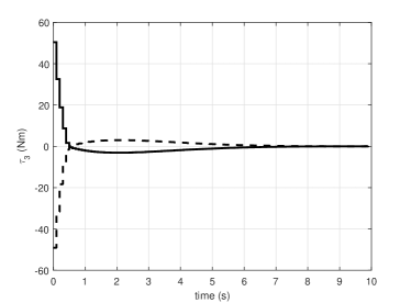
Figure 1: $\tau_{k,3}$ for initial rotation of 180 degrees (solid) and $-0.99\cdot 180$ (dotted)

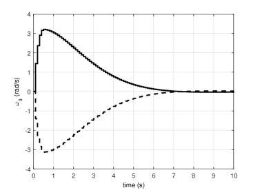
Figure 2: $\omega_{k,3}$ for initial rotation of 180 degrees (solid) and $-0.99\cdot 180$ (dotted)

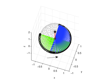
Figure 3: Orientation maneuver corresponding to the initial rotation of 180 degrees plotted at 2s increments

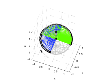
Figure 4: Orientation maneuver corresponding to the initial rotation of $-0.99\cdot 180$ degrees plotted at 2s increments

6 Conclusion

This paper presented a general MPC theory for dynamics that evolve on smooth manifolds. An MPC scheme was developed for manifolds that generalizes the results of conventional MPC in the case of $\mathbb{R}^{n}$. In the case of MPC on manifolds, a general construction for a locally valid control law on manifolds was derived, which was used in the design of the MPC terminal cost and target set.

Results were presented that showed the globally stabilizing properties of the MPC scheme as well as the nonexistence of continuous discrete-time control laws on manifolds whose Euler characteristic is not equal to 1. Thus, MPC achieves stability by producing a discontinuous control law, even in cases where a continuous globally stabilizing law does not exist. The authors believe that the ability to generate, possibly discontinuous, stabilizing feedback control laws for systems whose dynamics evolve on manifold is appealing for practical applications.

Finally, an application of the results to a constrained spacecraft attitude control problem was presented in the case of the matrix Lie group $\textrm{SO}(3)$. The simulation results that were presented showed the expected discontinuity in the MPC law.

Appendix A Proof of Theorem 1

In order to prove Theorem 1, we rely on discrete-time Lyapunov stability theory for smooth manifolds. Therefore, we begin by presenting the Lyapunov stability analysis. Let $M$ be an $n$-dimensional smooth manifold with metric $d$. Consider the following discrete-time dynamical system,

$$x_{k+1}=f(x_{k}),$$ (29)

where $x_{k}\in M$ and $f:M\to M$ is a continuous function.

Definition 2

A point $x_{e}\in M$ is called an equilibrium point of (29) if $f(x_{e})=x_{e}$.

Note that if $f(x_{e})=x_{e}$, then $f^{k}(x_{e})=x_{e}$, for all $k\in\mathbb{Z}_{+}$, where $f^{k+1}=f\circ f^{k}$ for all $k\in\mathbb{Z}_{+}$ and $f^{0}=\operatorname{id}_{M}$.

Definition 3

An equilibrium point $x_{e}\in M$ is said to be Lyapunov stable if for any open neighborhood ${U}\subset M$ of $x_{e}$, there exists an open neighborhood ${W}\subset M$ of $x_{e}$ such that for all $x_{0}\in{W}$, $f^{k}(x_{0})\in{U}$, for all $k\in\mathbb{Z}_{+}$. It is said to be locally asymptotically stable if it is Lyapunov stable and for all $x_{0}\in W$, $\lim_{k\to\infty}f^{k}(x_{0})=x_{e}$ or, equivalently, $\lim_{k\to\infty}d(f^{k}(x_{0}),x_{e})=0$.

Definition 4

Let $x_{e}$ be an equilibrium point of (29). A function $\mathcal{V}:M\to\mathbb{R}$ is a Lyapunov function if there exist two class-$\mathcal{K}$ functions $\alpha_{1},\alpha_{2}$, that satisfy $\alpha_{1}(d_{e}(x))\leq\mathcal{V}(x)\leq\alpha_{2}(d_{e}(x))$ for all $x$ in some neighborhood of $x_{e}$, and $\Delta\mathcal{V}(x)\colonequals\mathcal{V}(f(x))-\mathcal{V}(x)$ is negative semi-definite in a neighborhood of $x_{e}$. If $\Delta\mathcal{V}(x)$ is negative definite in a neighborhood of $x_{e}$, then $\mathcal{V}$ is a strict Lyapunov function.

More formally, the above definition implies that $\mathcal{V}$ is a Lyapunov function if there exists a neighborhood ${V}$ of $x_{e}$ such that $\mathcal{V}(x)>0$, $\Delta\mathcal{V}(x)\leq 0$ for all $x\in{V}\setminus\{x_{e}\}$, and $\mathcal{V}(x_{e})=0$. If, instead of $\Delta\mathcal{V}(x)\leq 0$, the condition $\Delta\mathcal{V}(x)<0$ holds for all $x\in{V}\setminus\{x_{e}\}$, then the Lyapunov function is a strict Lyapunov function.

Theorem 8

Let $x_{e}$ be an equilibrium point of (29).

1. If there exists a Lyapunov function $\mathcal{V}$, then $x_{e}$ is Lyapunov stable.

2. If there exists a strict Lyapunov function $\mathcal{V}$, then $x_{e}$ is locally asymptotically stable.

Proof. The proof follows arguments similar to the one given for the continuous-time case in [20].

1. Let $U\subset M$ be a neighborhood of $x_{e}$. As a consequence of Lemma 2.23 in [14], $M$ admits a locally finite cover by precompact sets, implying that there exists a neighborhood $U^{\prime}\subset M$ of $x_{e}$ that is a subset of the union of finitely many precompact sets, and therefore is itself precompact. Let $U^{\prime\prime}\subset U\cap U^{\prime}$ be an open neighborhood of $x_{e}$ on which $\alpha_{1}(d_{e}(x))\leq\mathcal{V}(x)\leq\alpha_{2}(d_{e}(x))$ for all $x\in U^{\prime\prime}$. Let $V_{\varepsilon}:=\{x\in M:d_{e}(x)\leq\varepsilon\}$ and choose $\varepsilon>0$ so that $V_{\varepsilon}$ is a subset of $U^{\prime\prime}$. By construction, $V_{\varepsilon}$ is a closed subset of a precompact set and is therefore compact. Let $V_{\varepsilon}(x_{e})\subset V_{\varepsilon}$ be the connected component of $V_{\varepsilon}$ containing $x_{e}$. The interior of $V_{\varepsilon}(x_{e})$ is non-empty and contains $x_{e}$. Let $x_{0}\in\operatorname{int}V_{\delta}(x_{e})$ where $\delta:=\alpha_{2}^{-1}(\alpha_{1}(\varepsilon))\leq\varepsilon$. Since $\mathcal{V}(x_{0})\leq\alpha_{2}(d_{e}(x_{0}))\leq\alpha_{2}(\delta)$ and $\mathcal{V}(f^{k}(x_{0}))-\mathcal{V}(x_{0})=\sum_{j=1}^{k}(\mathcal{V}(f^{j}(x_{0}))-\mathcal{V}(f^{j-1}(x_{0})))\leq 0$, it follows that $\mathcal{V}(f^{k}(x_{0}))\leq\mathcal{V}(x_{0})\leq\alpha_{2}(\delta)$, which implies that $d_{e}(f^{k}(x_{0}))\leq\alpha_{1}^{-1}(\mathcal{V}(f^{k}(x_{0})))\leq\alpha_{1}^{-1}(\alpha_{1}(\varepsilon))=\varepsilon$ for all $k\in\mathbb{Z}_{+}$. Because $V_{\varepsilon}$ is compact and $\mathcal{V}$ is positive definite in a neighborhood of $x_{e}$, there exists a constant $\varepsilon^{\prime}\leq\varepsilon$ such that $V_{\varepsilon^{\prime}}$ consists of only one connected component, so that $V_{\varepsilon^{\prime}}=V_{\varepsilon^{\prime}}(x_{e})$. As a consequence, for any neighborhood $U$, there exists $W=\operatorname{int}V_{\varepsilon^{\prime}}$ such that for any $x_{0}\in W$, $f^{k}(x_{0})\in U$ for all $k\in\mathbb{Z}_{+}$.

2. Let $U\subset M$ be a neighborhood of $x_{e}$. Choose $\varepsilon^{\prime}>0$ so that $\mathcal{V}$ is positive definite, $\Delta\mathcal{V}$ is strictly negative definite on $V_{\varepsilon^{\prime}}$, and $V_{\varepsilon^{\prime}}$ is a compact set with only one connected component. Let $W=\operatorname{int}V_{\varepsilon^{\prime}}$ as in the proof of (i), implying that $x_{e}$ is Lyapunov stable. For all $x_{0}\in W$, the sequence $\{\alpha_{1}(d_{e}(f^{k}(x_{0})))\}_{k\in\mathbb{Z}_{+}}$ is a non-increasing sequence bounded below by $0$, and hence $\lim_{k\to\infty}\alpha_{1}(d_{e}(f^{k}(x_{0})))=\beta\geq 0$. We can show that $\beta=0$ by contradiction. Assume $\beta>0$, implying that the set $V_{\varepsilon^{\prime}}\setminus\operatorname{int}V_{\alpha_{1}^{-1}(\beta)}$ does not contain $x_{e}$. Because this set is compact and does not contain $x_{e}$, the strictly negative definite, continuous function $\Delta\mathcal{V}$ attains a negative maximum on this set. Denote the maximum by $-\sigma<0$. For any $x_{0}\in W$, $\mathcal{V}(f^{k}(x_{0}))=\mathcal{V}(x_{0})+\sum_{j=1}^{k}(\mathcal{V}(f^{j}(x_{0}))-\mathcal{V}(f^{j-1}(x_{0})))\leq\mathcal{V}(x_{0})-k\sigma$. For any $k>\mathcal{V}(x_{0})/\sigma$, it follows that $\alpha_{1}(d_{e}(f^{k}(x_{0})))\leq\mathcal{V}(f^{k}(x_{0}))<0$, which contradicts the fact that $\alpha_{1}\circ d_{e}$ is positive definite. Therefore $\beta=0$ and, because $\alpha_{1}\circ d_{e}$ is continuous and positive definite, $\lim_{k\to\infty}f^{k}(x_{0})=x_{e}$.

Remark 5

Note that, because $f$ is a function whose domain and codomain are equal to $M$, $f^{k}$, where $k\in\mathbb{Z}_{+}$, is also a function whose domain and codomain are equal to $M$. Therefore, the existence and uniqueness of the sequence $\{f^{k}(x_{0})\}_{k\in\mathbb{Z}_{+}}$ is guaranteed for any $x_{0}\in M$.

Proof of Theorem 1. Given $x_{k}$, denote by $x_{k+i|k}^{*}$ the predicted state at time $k+i$ by (7) at time $k$.

Assume $x_{k}\in\mathcal{D}_{N}$ so that there exists an optimal sequence $\{u^{*}_{k|k},\dots,u^{*}_{k+N-1|k}\}$ solving (7). Together, $x_{k+1}=f(x_{k},u^{*}_{k|k})$ and $x^{*}_{k+N|k}\in\mathcal{X}_{T}$ imply that $\{u^{*}_{k+1|k},\dots,u^{*}_{k+N-1|k},\kappa(x^{*}_{k+N|k})\}$ is feasible for (7) at time $k+1$, which implies that $x_{k+1}\in\mathcal{D}_{N}$. Since $x_{0}\in\mathcal{D}_{N}$, then by induction, $x_{k}\in\mathcal{D}_{N}$ for all $k\in\mathbb{Z}_{+}$, proving (i).

For $x_{k}\in\mathcal{X}_{T}$, let $x_{k+i+1|k}=f(x_{k+i|k},\kappa(x_{k+i|k}))$ for $i\in\mathbb{Z}_{N}$ and $x_{k|k}=x_{k}$. Let $J_{\kappa}:\mathcal{X}_{T}\rightarrow\mathbb{R}$ be a function such that $J_{\kappa}(x_{k})=\mathcal{V}_{N}(x_{k},\{\kappa(x_{k+i|k})\}_{k\in\mathbb{Z}_{N}})$. The function $J_{\kappa}$ is positive definite on $\mathcal{X}_{T}$ and continuous, because $\kappa$ and $\mathcal{V}_{N}$ are continuous.

Let $J:\mathcal{D}_{N}\rightarrow\mathbb{R}$ be a function such that $J(x_{k})=\mathcal{V}_{N}^{*}(x_{k})$. Let $J^{*}=J|_{\mathcal{X}_{T}}$ be the restriction of $J$ to the domain $\mathcal{X}_{T}\subset\mathcal{D}_{N}$. Let $\alpha_{1}=\gamma+N\alpha$. To prove that $J^{*}$ is a Lyapunov function we use the following result.

Lemma 9

Let $J_{\kappa}:M\rightarrow\mathbb{R}$ be a function that is continuous and positive definite on a compact neighborhood $V\subset M$ of $x_{e}$. Then there exists a class-$\mathcal{K}$ function $\alpha_{2}$ such that $J_{\kappa}(x)\leq\alpha_{2}(d_{e}(x))$ for all $x\in V$.

Proof. Let $J_{m}(\delta)=\max_{x\in V}\{J_{\kappa}(x):d_{e}(x)\leq\delta\}$. By construction, $J_{m}$ is a continuous and non-decreasing function with domain $[0,a_{N_{a}}]$, where $0<a_{N_{a}}<\infty$, and satisfies $J_{m}(0)=0$. This implies that the domain can be decomposed into finitely many closed intervals $[0,a_{N_{a}}]=\cup_{i\in\mathbb{Z}_{N_{a}}}[a_{i},a_{i+1}]$, where $J_{m}(\delta)$ is strictly increasing on $[a_{i},a_{i+1}]$ when $i$ is even and $J_{m}(\delta)$ is constant on $[a_{i},a_{i+1}]$ when $i$ is odd.

Choose a small, positive scalar value $\sigma>0$. Let $\alpha_{2}(0)=0$, $\alpha_{2}(\delta)=\alpha_{2}(a_{i})-J_{m}(a_{i})+J_{m}(\delta)$ for $\delta\in[a_{i},a_{i+1}]$ when $i$ is even, and $\alpha_{2}(\delta)=\alpha_{2}(a_{i})+\sigma\frac{\delta-a_{i}}{a_{i+1}-a_{i}}$ for $\delta\in[a_{i},a_{i+1}]$ when $i$ is odd. By construction, $\alpha_{2}$ is a class-$\mathcal{K}$ function and $J_{m}(\delta)\leq\alpha_{2}(\delta)$ for all $\delta\in[0,a_{N_{a}}]$. Because $J_{\kappa}(x)\leq J_{m}(d_{e}(x))\leq\alpha_{2}(d_{e}(x))$ for all $x\in V$, the proof is complete.

According to the lemma, there exists a function $\alpha_{2}$ such that $\alpha_{1}(d_{e}(x))\leq J^{*}(x)\leq J_{\kappa}(x)\leq\alpha_{2}(d_{e}(x))$ for all $x\in\mathcal{X}_{T}$, where $\alpha_{1}$ and $\alpha_{2}$ are class-$\mathcal{K}$ functions.

By optimality, $J(x_{k+1})-J(x_{k})\leq-F(x_{k+N|k}^{*})-L(x_{k},u_{k})+F(x_{k+N+1|k}^{*})+L(x_{k+N|k}^{*},\kappa(x_{k+N|k}^{*}))\leq-L(x_{k},u_{k})\leq-\gamma(d(x_{k},x_{e}))$ for any $x_{k}\in\mathcal{D}_{N}$. This implies that $\gamma(d_{e}(x_{k}))\rightarrow 0$ as $k\rightarrow\infty$, and therefore $x_{k}\rightarrow x_{e}$ as $k\rightarrow\infty$ for any $x_{k}\in\mathcal{D}_{N}$. Therefore the equilibrium of $x_{e}$ is asymptotically stable and its domain of attraction is $\mathcal{D}_{N}$, proving (ii).

References

• [1] U. Kalabić, R. Gupta, S. Di Cairano, A. Bloch, I. Kolmanovsky, Constrained spacecraft attitude control on $\textrm{SO}(3)$ using reference governors and nonlinear model predictive control, in: Proc. American Control Conf., Portland, OR, 2014, pp. 5586–5593.
• [2] J. B. Rawlings, D. Q. Mayne, Model Predictive Control: Theory and Design, Nob Hill, Madison, WI, 2009.
• [3] H. Munthe-Kass, High order Runge-Kutta methods on manifolds, Appl. Numer. Math. 29 (1) (1999) 115–127.
• [4] J. E. Marsden, M. West, Discrete mechanics and variational integrators, Acta Numerica 10 (2001) 357–514.
• [5] E. Hairer, C. Lubich, G. Wanner, Geometric Numerical Integration, Springer-Verlag, Berlin, Germany, 2006.
• [6] T. Lee, Computational geometric mechanics and control of rigid bodies, Ph.D. thesis, University of Michigan, Ann Arbor (2008).
• [7] T. Lee, N. H. McClamroch, M. Leok, A Lie group variational integrator for the attitude dynamics of a rigid body with applications to the 3D pendulum, in: Proc. IEEE Int. Conf. Control Applicat., Toronto, ON, 2005, pp. 962–967.
• [8] T. Lee, M. Leok, N. H. McClamroch, Optimal attitude control of a rigid body using geometrically exact computations on $\textrm{SO}(3)$, J. Dynamical Control Syst. 14 (4) (2008) 465–487.
• [9] S. P. Bhat, D. S. Bernstein, A topological obstruction to continuous global stabilization of rotational motion and the unwinding phenomenon, Systems & Control Letters 39 (1) (2000) 63–70.
• [10] V. Guillemin, A. Pollack, Differential Topology, Prentice Hall, Englewood Cliffs, NJ, 1974.
• [11] Z. Nagy, R. Findeisen, M. Diehl, F. Allgöwer, H. Georg Bock, S. Agachi, J. P. Schlöder, D. Leineweber, Real-time feasibility of nonlinear predictive control for large scale processes - a case study, in: Proc. American Control Conf., Chicago, IL, 2000, pp. 4249–4253.
• [12] S. Gros, M. Zanon, M. Vukov, M. Diehl, Nonlinear MPC and MHE for mechanical multi-body systems with application to fast tethered airplanes, in: Proc. Nonlin. Model Predictive Control, Noordwijkerhout, Netherlands, 2012, pp. 86–93.
• [13] E. S. Meadows, M. A. Henson, J. W. Eaton, J. B. Rawlings, Receding horizon control and discontinuous state feedback stabilization, Int. J. Control 62 (5) (1995) 1217–1229.
• [14] J. M. Lee, Introduction to Smooth Manifolds, Springer, New York, 2013.
• [15] J. M. Milnor, Topology from the Differential Viewpoint, Princeton University Press, Princeton, NJ, 1997.
• [16] W. F. Arnold III, A. J. Laub, Generalized eigenproblem algorithms and software for algebraic Riccati equations, Proc. IEEE 72 (12) (1984) 1746–1754.
• [17] A. Granas, J. Dugundji, Fixed Point Theory, Springer, New York, 2003.
• [18] W. Lin, C. I. Byrnes, Design of discrete-time nonlinear control systems via smooth feedback, IEEE T. Automat. Control 39 (11) (1994) 2340–2346.
• [19] J. R. Cardoso, F. S. Leite, The Moser-Veselov equation, Linear Algebra Applicat. 360 (2003) 237–248.
• [20] F. Bullo, A. D. Lewis, Geometric Control of Mechanical Systems, Springer, New York, 2005.