Optimal Design of Networks of Positive Linear Systems
under Stochastic Uncertainty

Abstract

In this paper, we study networks of positive linear systems subject to time-invariant and random uncertainties. We present linear matrix inequalities for checking the stability of the whole network around the origin with prescribed probability and decay rate. Based on this condition, we then give an efficient method, based on geometric programming, to find the optimal parameters of the probability distribution describing the uncertainty. We illustrate our results by analyzing the stability of a viral spreading process in the presence of random uncertainties.

I Introduction

Stability analysis of uncertain dynamical systems or, precisely speaking, dynamical systems with tine-invariant and uncertain parameters, has attracted extensive attention for a long time in systems and control theory. In particular, for the stability analysis of uncertain linear systems, there have been proposed various tools including generalized Kharitonov’s theorem [1], common quadratic Lyapunov functions [2], parameter-dependent quadratic lyapunov functions [3, 4], and parameter-dependent polynomial Lyapunov functions [5, 6, 7]. For positive linear systems, which are the class of linear systems whose state variable is nonnegative entrywise provided the initial state is, the authors in [8] and [9] propose robust stability conditions based on diagonal Lyapunov functions [10] and linear storage functions, respectively.

All the works mentioned above model the uncertainty of a linear system by providing a set of all possible configurations of the system. This is done typically via polytopes where coefficient matrices of the system can belong to. We can find in the literature several contribution to determine whether the uncertain system is stable for all possible configurations or not. An important consequence is that, in these frameworks, all possible system configurations are equally important. However, in some applications, we are able to give not only the set of possible uncertain parameters but also a weight, typically a probability distribution, that measures the relative importance of the elements in the uncertainty set.

One of the earliest works along this line is presented in [11], where the authors analyze the stability of linear time-invariant systems whose coefficient matrices are modeled via a random vector. Using first- and second-order reliability methods [12], the authors analyze the stability of specific mechanical systems, and also study the probability of the system being stable with respect to physical parameters, such as stiffness and damping ratio. They also compare various control strategies such as those based on linear quadratic regulator and Kalman filters. However, their results are limited to the analysis of low-order systems and cannot be easily generalized to the case of possibly large networks composed by uncertain systems.

In this paper, we present a robust stability analysis for networks of positive linear systems subject to time-invariant and random uncertainty. We first present linear matrix inequalities for checking if a given network of uncertain positive linear systems is stable with a given probability and a decay rate. Based on this result, we then present a convex optimization problem, posed as a geometric program [13], for optimally designing the parameters of the probability distribution expressing the uncertainty. We illustrate the obtained results using a networked susceptible-infected-susceptible epidemic model [14], which has found applications in, for example, public health [15], malware spreading [16], and information propagation over socio-technical networks [17]. The results in this paper are based on the probabilistic estimate [18] for the maximum real eigenvalue of random and symmetric matrices.

This paper is organized as follows. After introducing necessary notations, in Section II we introduce our model of the network of uncertain positive linear systems and then state the problems to be studied. We then propose a convex optimization framework for analyzing the stability of random networks in Section III. Based on this analysis, we study the optimal design of the probability distributions describing uncertainties in Section IV. Numerical examples are presented in Section V.

I-A Mathematical Preliminaries

We denote by $\mathbb{R}$ the set of real numbers. The set $\{1,\ldots,N\}$ is denoted by $[N]$. For vectors $x,y\in\mathbb{R}^{N}$, we write $x\geq y$ ($x>y$) if $x_{i}\geq y_{i}$ ($x_{i}>y_{i}$, respectively) for every $i\in[N]$. We say that $x$ is positive if $x>0$. We denote the identity matrix by $I$. A square matrix is said to be Metzler if its off-diagonal entries are nonnegative. The Kronecker product of the matrices $A$ and $B$ is denoted by $A\otimes B$. The direct sum of the matrices $A_{1}$, $\dotsc$, $A_{N}$, denoted by $\bigoplus_{i=1}^{N}A_{i}$, is defined as the block-diagonal matrix containing the matrices  $A_{1}$, $\dotsc$, $A_{N}$ as its diagonal blocks. When a symmetric matrix $A$ is positive semi-definite, we write $A\succeq 0$. For another symmetric matrix $B$, we write $A\succeq B$ if $A-B\succeq 0$. The notations $A\succ B$ and $A\preceq B$ are defined in the obvious way. If $A\succeq 0$, then $\sqrt{A}$ denotes a (not necessarily unique) matrix such that $A={\sqrt{A}}(\sqrt{A})^{\top}$ holds. For a random matrix $M$, we denote its expectation by $E[M]$. The variance of $M$ is given by $\operatorname{Var}(M)=E[(M-E[M])^{2}]$. Also we define the positive semi-definite matrix

$$W(M)=E[M^{\top}M]-E[M]^{\top}E[M].$$

The symbol $\star$ is used to denote the symmetric blocks of partitioned symmetric matrices.

The design framework proposed in this paper depends on a class of optimization problems called geometric programs [13]. Let $x_{1}$, $\dotsc$, $x_{n}$ denote positive variables and define ${x}=(x_{1},\dotsc,x_{n})$. We say that a real-valued function $g({x})$ is a monomial function if there exist $c\geq 0$ and $a_{1},\dotsc,a_{n}\in\mathbb{R}$ such that $g({x})=cx_{\mathstrut 1}^{a_{1}}\dotsm x_{\mathstrut n}^{a_{n}}$. Also we say that a function $f({x})$ is a posynomial function if it is a sum of monomial functions of ${x}$. For information about the modeling power of posynomial functions, we point the readers to [13]. Given a collection of posynomial functions $f_{0}{(x)}$, $\dotsc$, $f_{p}{(x)}$ and monomials $g_{1}{(x)}$, $\dotsc$, $g_{q}{(x)}$, the optimization problem

$$\operatorname*{minimize}_{x} f_{0}({x})$$

$$\operatorname*{subject\ to} f_{i}({x})\leq 1,\quad i=1,\dotsc,p,$$

$$g_{j}({x})=1,\quad j=1,\dotsc,q,$$

is called a geometric program. Although geometric programs are not convex, they can be efficiently converted into a convex optimization problem.

II Problem formulation

In this section, we introduce the model of the network of linear systems with stochastic uncertainty. We then state the problems studied in this paper. Consider linear time-invariant and random systems

$$\Sigma_{i}:\frac{dx_{i}}{dt}=A_{ii}x_{i}+\sum_{j\neq i}A_{ij}x_{j},\quad i=1,\dotsc,N,$$ (1)

where $A_{ij}$ is an $\mathbb{R}^{n\times n}$-valued random matrix for all $i,j\in[N]$. We emphasize that $\Sigma_{i}$ is a linear time-invariant system for each realization of the random matrices $A_{ij}$. In other words, the coefficient matrices of $\Sigma_{i}$ do not change over time once they are chosen from the corresponding distributions.

If we introduce the notations

$$\begin{gathered}x=\begin{bmatrix}x_{1}\\ \vdots\\ x_{N}\end{bmatrix},\ A=\begin{bmatrix}A_{11}&\cdots&A_{1N}\\ \vdots&\ddots&\vdots\\ A_{N1}&\cdots&A_{NN}\\ \end{bmatrix},\end{gathered}$$

then, from (1), we obtain the random linear time-invariant system

$$\Sigma:\frac{dx}{dt}=Ax.$$

Following the deterministic case [19], we say that $\Sigma$ is positive if $x(0)=x_{0}\geq 0$ implies $x(t)\geq 0$ for every $t\geq 0$ with probability one.

The first problem we address in this paper is the following stability analysis problem with a prescribed decay rate and an unreliability level:

Problem II.1 (Stability analysis)

Given a desired decay rate $\lambda>0$ and an unreliability level $\epsilon\in(0,1]$, determine if, with probability at least $1-\epsilon$, the system $\Sigma$ is stable with decay rate $\lambda$.

We also investigate design problems. We assume that, though we cannot tune the values of the random variables $A_{ij}$ directly, we can still design their probability distributions. Specifically, we assume that the probability distributions of the random matrices $A_{ij}$ are parametrized by scalar parameters $r_{1}$, $\dotsc$, $r_{m}$ that we can design. Our design problem is based on cost functions and constraints. We suppose that there exists a function $R(r,\epsilon)$ that represents the cost for realizing the specific parameter $r$ and from allowing the unreliability level $\epsilon$. Also, for functions $\theta_{1}$, $\dotsc$, $\theta_{p}$, $\phi_{1}$, $\dotsc$, $\phi_{q}$ of $r$ and $\epsilon$, we allow the constraints on $r$ and $\epsilon$ of the form $f_{k}(r,\epsilon)\leq 1$ ($k=1,\dotsc,p$) and $g_{\ell}(r,\epsilon)=1$ ($\ell=1,\dotsc,q$). Now we can formulate the design problems studied in this paper:

Problem II.2 (Optimal design)

Given a desired decay rate $\lambda>0$, a cost bound $\bar{R}>0$, and an unreliability level $\epsilon\in(0,1]$, find the parameter $r$ such that the following conditions hold:

• With probability at least $1-\epsilon$, the system $\Sigma$ is stable with decay rate $\lambda$;

• The constraints $R(r,\epsilon)\leq\bar{R}$, $f_{k}(r,\epsilon)\leq 1$ ($k\in[p]$), and $g_{\ell}(r,\epsilon)=1$ ($\ell\in[q]$) are satisfied.

For solving the above stated problems, we place one of the following assumptions reflecting the networked-structure of the system $\Sigma$:

1. The random variables $\{A_{ij}\}_{i,j\in[N]}$ are independent;

2. The systems $\{\Sigma_{i}\}_{i\in[N]}$, i.e., the sets of random variables $\{A_{i1},\dotsc,A_{iN}\}_{i\in[N]}$, are independent.

Finally, to the networked system $\Sigma$, we associate a directed graph $(\mathscr{V},\mathscr{E})$ with $\mathscr{V}=[N]$ as follows. An ordered pair $(i,j)$, called a directed edge, is in $\mathscr{E}$ if $A_{ij}$ is not the zero random variable. We define the closed neighborhoods of $i$ by ${\mathscr{N}}^{-}[i]=\{j\in[N]:(i,j)\in\mathscr{E}\}$ and ${\mathscr{N}}^{+}[i]=\{j\in[N]:(j,i)\in\mathscr{E}\}$, respectively.

III Stability Analysis

In this section, we present the solutions of the stability analysis problem. We first state the results in Subsection III-A. The proof of the results is then presented in Subsection III-B.

III-A Stability Conditions

Throughout the paper, for an unreliability level $\epsilon\in(0,1]$, we define

$$\rho=\log(nN/\epsilon).$$

The next theorem gives a solution for the stability analysis problem under condition A1):

Theorem III.1

Suppose that A1) holds true. Let $\lambda>0$ and $\epsilon\in(0,1]$. Assume that there exist positive numbers $p_{1}$, $\dotsc$, $p_{N}$, $a$, $\Delta$, and $\sigma$ satisfying the linear matrix inequalities:

$$E[A]^{\top}P+PE[A]+aI+\lambda P\preceq 0,$$ (2a)

$$\begin{bmatrix}a-\frac{\rho}{3}\Delta&\sqrt{2\rho}\sigma&\frac{\rho}{3}\Delta\\ \star&a-\frac{\rho}{3}\Delta&0\\ \star&\star&a-\frac{\rho}{3}\Delta\end{bmatrix}\succ 0,$$ (2b)

$$p_{i}\operatorname{ess\,sup}\lVert A_{ij}-E[A_{ij}]\rVert\leq\Delta,$$ (2c)

$$\begin{bmatrix}\sigma I&p_{i}Q_{i}&R_{i}\\ \star&\sigma I&O\\ \star&\star&\sigma I\end{bmatrix}\succeq 0,$$ (2d)

where $P=\bigoplus_{i=1}^{N}(p_{i}I_{n})$, and $Q_{i},R_{i}$ are given for each $i\in[N]$ by

$$Q_{i}=\sqrt{\mathstrut\smash{\sum_{j\in\mathscr{N}^{+}[i]}}W(A_{ij}^{\top})},\quad R_{i}=\operatorname*{col}\bigl{(}p_{j}\sqrt{\mathstrut W(A_{\smash{ji}})}\bigr{)}_{j\in\mathscr{N}^{-}[i]},\vspace{.1cm}$$ (3)

with $\operatorname*{col}(\cdot)$ denoting the column vector obtained by stacking its arguments. Then, with probability at least $1-\epsilon$, the system $\Sigma$ is stable with decay rate $\lambda$. Moreover, if linear matrix inequalities (2) are solvable for an $\epsilon=\epsilon_{1}$, then so are for every $\epsilon\geq\epsilon_{1}$.

Several remarks on Theorem III.2 are in order. Though feasibility of linear matrix inequalities (2) implies the stability of the averaged system $dx/dt=E[A]x$ with exponential convergence rate $\lambda$ due to (2a), the converse is not necessarily true mainly by the additional term $aI$ in the left hand side of (2a). Also notice that the coefficient $a$ of the additional is related through (2b) to $\Delta$ and $\sigma$, which quantify the variability of the random system $\Sigma$ as can be seen from the proof of the theorem. Finally, the last claim of the theorem implies that a bisection search effectively finds the minimum unreliability level given by

$$\epsilon^{\star}=\inf\{\epsilon>0:\text{\eqref{eq:stbl:analysis:iid} is solvable}\}.$$ (4)

Then we consider the condition A2). For each $i\in[N]$, define the $\mathbb{R}^{n\times(nN)}$-valued random matrix $A_{i}=\begin{bmatrix}A_{i1}&\cdots&A_{iN}\end{bmatrix}$. Then, define the $\mathbb{R}^{(nN)\times(nN)}$-valued random matrix $S_{i}=e_{i}^{\top}\otimes A_{i}^{\top}+e_{i}\otimes A_{i}$ for each $i\in[N]$, where $e_{i}$ denotes the $i$th standard unit vector in $\mathbb{R}^{N}$. Then, the next theorem gives a solution to the stability analysis problem under condition A2):

Theorem III.2

Suppose that A2) holds true. Let $\lambda>0$ and $\epsilon\in(0,1]$. Assume that there exist positive numbers $p_{1}$, $\dotsc$, $p_{N}$, $a$, $\sigma$, and $\Delta$ satisfying the linear matrix inequalities:

$$\text{\eqref{eq:lmi:main} and \eqref{eq:LMI:aDeltarho}},$$ (5a)

$$2p_{i}\operatorname{ess\,sup}\lVert A_{i}-E[A_{i}]\rVert\leq\Delta,$$ (5b)

$$\begin{bmatrix}\sigma I&p_{1}\sqrt{\operatorname{Var}(S_{1})}&\cdots&p_{N}\sqrt{\operatorname{Var}(S_{N})}\\ \star&\sigma I&&\\ \vdots&&\ddots\\ \star&&&\sigma I\end{bmatrix}\succeq 0.$$ (5c)

Then, with probability at least $1-\epsilon$, the system $\Sigma$ is stable with decay rate $\lambda$. Moreover, if linear matrix inequalities (5) are solvable for an $\epsilon=\epsilon_{1}$, then so are for every $\epsilon\geq\epsilon_{1}$.

Remark III.3

By the structure of matrix $S_{i}$ and the definition of the graph $\mathscr{V}$, the positive semi-definite matrix $\operatorname{Var}(S_{i})$ has rank at most $nd^{-}[i]$. Therefore, we can take the square root $\sqrt{\operatorname{Var}(S_{i})}$ having at most $nd^{-}[i]$ rows.

III-B Proof

For the proof of Theorems III.1 and III.2, we recall the following probabilistic estimate on the maximum eigenvalue of the sum of random and symmetric matrices:

Proposition III.4 ([18])

For two positive constants $\Delta$ and $\sigma$, define the function

$$\kappa_{\Delta,\sigma^{2}}(a)=n\exp\left(-\frac{a^{2}}{2\sigma^{2}+\frac{2\Delta a}{3}}\right),\ a\geq 0.$$

Let $X_{1}$, $\dotsc$, $X_{N}$ be independent random $n\times n$ symmetric matrices. Let $\Delta$ be a nonnegative constant such that $\lVert X_{i}-E[X_{i}]\rVert\leq\Delta$ for every $i\in[N]$ with probability one. Also take an arbitrary $\sigma\geq 0$ satisfying $\lVert\sum_{i=1}^{N}\operatorname{Var}(X_{i})\rVert\leq\sigma^{2}$. Then, the sum $X=\sum_{i=1}^{N}X_{i}$ satisfies

$$P\left(\eta(X)\geq\eta(E[X])+a\right)<\kappa_{\Delta,\sigma^{2}}(a)$$

for every $a>0$.

About the function $\kappa_{\Delta,\sigma^{2}}$ appearing in this proposition, we can prove the following straightforward but yet important lemma:

Lemma III.5

For all positive numbers $\Delta$, $\sigma$, $a$, and $\epsilon$, the following statements are equivalent:

1. $\kappa_{\Delta,\sigma^{2}}(a)<\epsilon$;

2. $2\rho\Delta a^{-1}+6\rho\sigma^{2}a^{-2}<3$;

3. The matrix inequality (2b) holds.

Moreover, for fixed $\Delta$, $\sigma$, and $a$, if one of the above equivalent statements is satisfied by an $\epsilon=\epsilon_{1}$, then the statements are satisfied for every $\epsilon\geq\epsilon_{1}$.

Proof:

Taking the logarithm in the both hand sides of the inequality $\kappa_{\Delta,\sigma^{2}}(a)<\epsilon$ immediately gives the equivalence [1) $\Leftrightarrow$ 2)]. Also, the equivalence [2) $\Leftrightarrow$ 3)] readily follows from taking the Schur complement of the matrix in the inequality (2b) with respect to its $(1,1)$-entry. Then, the latter claim about the monotonicity follows from the fact that the left hand side of the inequality in 2) is increasing with respect to $\rho$ and therefore decreasing with respect to $\epsilon$. ∎

Let us prove Theorem III.1.

Proof of Theorem III.1: Assume that positive numbers $p_{1}$, $\dotsc$, $p_{N}$, $a$, $\Delta$, and $\sigma$ solve linear matrix inequalities (2). Let $X_{ij}=p_{i}(U_{ji}\otimes A_{ij}^{\top}+U_{ij}\otimes A_{ij})$, where $U_{ij}\in\mathbb{R}^{N\times N}$ denotes the $\{0,1\}$-matrix elements are all zero except its $(i,j)$-entry. Then, from the basic property of Kronecker products of matrices [20], we obtain $A^{\top}P+PA+\lambda P=\lambda P+\sum_{i=1}^{N}\sum_{j=1}^{N}X_{ij}$, to which we apply Proposition III.4. By (2c), we can derive the estimate

$$\lVert X_{ij}-E[X_{ij}]\rVert =\begin{multlined}p_{i}\Bigl{\lVert}U_{ji}\otimes(A_{ij}-E[A_{ij}])^{\top}+\\ U_{ji}\otimes(A_{ij}-E[A_{ij}])\Bigr{\rVert}\end{multlined}p_{i}\Bigl{\lVert}U_{ji}\otimes(A_{ij}-E[A_{ij}])^{\top}+\\ U_{ji}\otimes(A_{ij}-E[A_{ij}])\Bigr{\rVert}$$

$$=p_{i}\lVert A_{ij}-E[A_{ij}]\rVert$$

$$\leq\Delta.$$

Also, since a straightforward computation shows

$$\operatorname{Var}(X_{ij})=p_{i}^{2}(U_{jj}\otimes(A_{ij}^{\top}A_{ij})+U_{ii}\otimes(A_{ij}A_{ij}^{\top})),$$

we have

$$\sum_{i=1}^{N}\sum_{j=1}^{N}\operatorname{Var}(X_{ij})=\sum_{i=1}^{N}U_{ii}\otimes\left(\sum_{j=1}^{N}(p_{j}^{2}W(A_{ji})+p_{i}^{2}W(A_{ij}^{\top}))\right).$$

Therefore, by (2d) and the definition (3) of the matrices $Q_{i}$ and $R_{i}$,

$$\left\lVert\sum_{i=1}^{N}\sum_{j=1}^{N}\operatorname{Var}(X_{ij})\right\rVert =\max_{1\leq i\leq N}\left\lVert p_{i}^{2}\sum_{j=1}^{N}W(A_{ij}^{\top})+\sum_{j=1}^{N}p_{j}^{2}W(A_{ji})\right\rVert$$

$$=\max_{1\leq i\leq N}\left\lVert(p_{i}Q_{i})(p_{i}Q_{i})^{\top}+R_{i}R_{i}^{\top}\right\rVert$$

$$\leq\sigma^{2}.$$

Now, by Proposition III.4, we have

$$\begin{multlined}P\Bigl{(}\lambda_{\max}(A^{\top}P+PA+\lambda P)\geq\\ \lambda_{\max}(E[A]^{\top}P+PE[A]+\lambda P)+a\Bigr{)}<\kappa_{\Delta,\sigma^{2}}(a).\end{multlined}P\Bigl{(}\lambda_{\max}(A^{\top}P+PA+\lambda P)\geq\\ \lambda_{\max}(E[A]^{\top}P+PE[A]+\lambda P)+a\Bigr{)}<\kappa_{\Delta,\sigma^{2}}(a).$$

By (2b) and Proposition III.5, we have $\kappa_{\Delta,\sigma^{2}}(a)<\epsilon$. Therefore, the inequality (2a) implies that $P\bigl{(}\lambda_{\max}(A^{\top}P+PA+\lambda P)\geq 0\bigr{)}<\epsilon$. This shows that, with probability at least $1-\epsilon$, we have that $A^{\top}P+PA+\lambda P<0$. This means that, with probability at least $1-\epsilon$, the system $\Sigma$ has the Lyapunov function $V(x)=x^{\top}Px$ with decay rate $\lambda$. This completes the proof of the first part of the theorem.

Let us then prove the second statement of the theorem. Let $\epsilon_{1}>0$ be arbitrary and assume that linear matrix inequalities (2) are solvable when $\epsilon=\epsilon_{1}$ with the parameters $p_{1}$, $\dotsc$, $p_{N}$, $a$, $\lambda$, $\Delta$, and $\sigma$. We show that, with the same parameters, inequalities (2) are solvable whenever $\epsilon\geq\epsilon_{1}$. By the choice of the parameters, all the linear matrix inequalities in (2) except (2b) hold true. Also, the feasibility of (2b) follows from the latter claim in Lemma III.5. This completes the proof of the theorem.

Remark III.6

As can be observed from the above proof, in Theorem III.1, we confine our attention to the Lyapunov functions $x^{\top}Px$ with diagonal $P$. This choice is motivated by the following fact [10]: a positive linear system $dx/dt=Ax$ is stable if and only if it admits a Lyapunov function $x^{\top}Px$ with diagonal $P\succ 0$. Also notice that we use the diagonal matrix $P\in\mathbb{R}^{(nN)\times(nN)}$ determined by only $N$ parameters $p_{1}$, $\dotsc$, $p_{N}$. Using the fully parametrized diagonal matrix $P$ would yield a less conservative result than the theorem. In this paper, we however choose not to present the fully parametrized case to keep presentation simple.

We then give the proof of Theorem III.2.

Proof of Theorem III.2: Assume that positive numbers $p_{1}$, $\dotsc$, $p_{N}$, $a$, $\lambda$, $\sigma$, and $\Delta$ solve linear matrix inequalities (5). Let $X_{i}=p_{i}S_{i}$. Then we have $A^{\top}P+PA+\lambda P=\lambda P+\sum_{i=1}^{N}X_{i}$, to which we again apply Proposition III.4 as in the proof of Theorem III.1. By (5b), we can show that

$$\lVert X_{i}-E[X_{i}]\rVert =p_{i}\left\lVert e_{i}^{\top}\otimes(A_{i}-E[A_{i}])^{\top}+e_{i}\otimes(A_{i}-E[A_{i}])\right\rVert$$

$$\leq 2p_{i}\lVert e_{i}\otimes(A_{i}-E[A_{i}])\rVert$$

$$=2p_{i}\lVert A_{i}-E[A_{i}]\rVert$$

$$\leq\Delta.$$

Also, the inequality (5c) immediately shows $\lVert\sum_{i=1}^{N}\operatorname{Var}(X_{i})\rVert=\lVert\sum_{i=1}^{N}p_{i}^{2}\operatorname{Var}(S_{i})\rVert\leq\sigma^{2}$. The rest of the proof is the same that of Theorem III.1 and hence is omitted.

IV Optimal Design

Based on Theorems III.1 and III.2, in this section we study network design problems. Roughly speaking, designing the distributions of $A$ or, the parameters $r_{1}$, $\dotsc$, $r_{m}$, corresponds to solving matrix inequalities (2) or (5) with $E[A]$ being a variable. This in particular makes the inequalities not linear with respect to decision variables. To avoid the difficulty, in this paper we employ geometric programming [13] instead of linear matrix inequalities. For this purpose, we place the following assumptions on the random coefficient matrices of $\Sigma$:

1. There exist random variables $A_{+}$ and $A_{-}$ satisfying $A=A_{+}-A_{-}$ such that $E[A_{+}]$ is a posynomial matrix and $E[A_{-}]$ is a diagonal monomial matrix in variables $r_{1}$, $\dotsc$, $r_{m}$;

2. The cost function $R$ and the constraint functions $f_{1}$, $\dotsc$, $f_{p}$ are posynomial functions in $r_{1}$, $\dotsc$, $r_{m}$, and $\rho$.

3. The constraint functions $g_{1}$, $\dotsc$, $g_{q}$ are monomials in $r_{1}$, $\dotsc$, $r_{m}$, and $\rho$.

Under this assumption, the next theorem gives a solution to the stabilization problem for the case A1) holds:

Theorem IV.1

Suppose that $\Sigma$ is positive and A1) holds true. For all $i,j\in[N]$, let $\eta_{i}$, $\Phi_{ij}$ $\Psi_{ij}$ be posynomial functions in $r_{1}$, $\dotsc$, $r_{m}$ such that

$$\begin{gathered}\operatorname{ess\,sup}\lVert A_{ij}-E[A_{ij}]\rVert\leq\eta_{ij},\\ W(A_{ij})\preceq\Phi_{ij},\quad W(A_{ij}^{\top})\preceq\Psi_{ij}.\end{gathered}$$ (6)

Assume that the following geometric program is feasible:

$$\operatorname*{minimize}_{\begin{subarray}{c}a,\,\Delta,\,\sigma,\,\rho,\,\lambda\in\mathbb{R},\\ p\in\mathbb{R}^{N},\,r\in\mathbb{R}^{m},\\ v\in\mathbb{R}^{nN},\,w_{i}\in\mathbb{R}^{n}\end{subarray}}\, 1/\lambda$$ (7a)

$$\operatorname*{subject\ to}\ (E[A_{+}^{\top}]P\!+\!PE[A_{+}]\!+\!aI\!+\!\lambda P)v\leq 2PE[A_{-}]v,$$ (7b)

$$2\rho\Delta a^{-1}+6\rho\sigma^{2}a^{-2}<3,$$ (7c)

$$p_{i}\eta_{ij}(r)\leq\Delta,$$ (7d)

$$\left(p_{i}^{2}\sum_{j=1}^{N}\Psi_{ij}(r)+\sum_{j=1}^{N}p_{j}^{2}\Phi_{ji}(r)\right)w_{i}\leq\sigma^{2}w_{i},$$ (7e)

$$R(r,\epsilon(\rho))\leq\bar{R},$$ (7f)

$$f_{k}(r,\epsilon(\rho))\leq 1,\ g_{\ell}(r,\epsilon(\rho))=1.$$ (7g)

Let $\rho^{\star}$, $r^{\star}$, and $\lambda^{\star}$ be the optimal solution of this optimization problem. Define $\epsilon^{\star}=nN/e^{-\rho^{\star}}$. Then, with probability at least $1-\epsilon^{\star}$, the system $\Sigma$ with parameters $r^{\star}$ is stable with decay rate $\lambda^{\star}$.

Proof:

Conditions B1)–B3) guarantee the optimization problem (7) to be a geometric program. Assume that the optimization problem (7) is feasible. We show that the linear matrix inequalities (2) are feasible. The inequality (7b) implies that $(E[A]^{\top}P+PE[A]+aI+\lambda P)v\leq 0$. Since the matrix $E[A]^{\top}P+PE[A]+aI+\lambda P$ is Metzler by the positivity of $\Sigma$, the Perron-Frobenius theory and (7b) show that the matrix is negative semi-definite, i.e., the linear matrix inequality (2a) holds. By Proposition III.5, the inequality (7c) equivalently implies (2b). Also, the inequality (7d) and the definition of $\eta_{ij}$ show (2c). Furthermore, the inequality (7e) and (6) imply (2d). Hence, by Theorem III.2, we obtain the conclusion. ∎

Then, the next theorem gives a solution for the stabilization problem under A2):

Theorem IV.2

Suppose that $\Sigma$ is positive and A2) holds true. For each $i\in[N]$, let $\eta_{i}$ and $\Phi_{i}$ be posynomial functions in $r$ such that

$$\operatorname{ess\,sup}\lVert A_{i}-E[A_{i}]\rVert\leq\eta_{i},\quad\operatorname{Var}(S_{i})\preceq\Phi_{i}(r),$$

for every feasible $r$. Assume that the following geometric program is feasible:

$$\operatorname*{minimize}_{\begin{subarray}{c}a,\,\Delta,\,\sigma,\,\rho,\,\lambda\in\mathbb{R},\\ p\in\mathbb{R}^{N},\,r\in\mathbb{R}^{m},\,v,w_{i}\in\mathbb{R}^{nN}\end{subarray}} 1/\lambda$$

$$\operatorname*{subject\ to} \text{\eqref{eq:gp:main:iid}, \eqref{eq:gp:s:iid}, \eqref{eq:gp:cost}, and \eqref{eq:gp:constraints}},$$

$$2p_{i}\eta_{i}(r)\leq\Delta,$$

$$\left(\sum_{i=1}^{N}p_{i}^{2}\Phi_{i}(r)\right)w_{i}\leq\sigma^{2}w_{i}.$$

Let $\rho^{\star}$, $r^{\star}$, and $\lambda^{\star}$ be the solutions of this optimization problem. Define $\epsilon^{\star}=nN/e^{-\rho^{\star}}$. Then, with probability at least $1-\epsilon^{\star}$, the system $\Sigma$ with parameter $r^{\star}$ is stable with decay rate $\lambda^{\star}$.

Proof:

The proof is almost the same as the proof of Theorem IV.1 and hence is omitted. ∎

V Numerical Example

In this section, we illustrate the obtained results using a famous disease-spreading model in epidemiology called the heterogeneous networked susceptible-infected-susceptible model [14]. In the model, the evolution of the disease in a networked population whose graph has the adjacency matrix $A_{G}=[a_{ij}]_{i,j}\in\{0,1\}^{N\times N}$ is described as

$$\frac{dx_{i}}{dt}=-\delta_{i}x_{i}+\sum_{j=1}^{N}\beta_{ij}a_{ij}x_{j},\quad i\in[N],$$ (8)

where $\beta_{ij}$ and $\delta_{i}$ are positive constants. The variable $x_{i}(t)$ represents the probability that node $i$ is infected at time $t$. The constant $\beta_{ij}$, called the transmission rate, indicates the rate at which the infection is transmitted to node $i$ from its infected neighbor $j$. The constant $\delta_{i}$, called the recovery rate, indicates the rate at which the infection is cured. Define $B=[\beta_{ij}a_{ij}]_{i,j}\in\mathbb{R}^{N\times N}$ and $D=\operatorname{diag}(\delta_{1},\dotsc,\delta_{N})$. Then, the dynamics in (8) are written by the differential equation

$$\frac{dx}{dt}=(B-D)x,$$ (9)

whose stability indicates that the infection will be eradicated asymptotically.

Assume that we have an access to preventative resource that can change the natural transmission rate, denoted by $\bar{\beta}_{ij}$ to another rate $\underaccent{\bar}{\beta}_{ij}$ smaller than $\bar{\beta}_{ij}$. We consider the situation that, though the preventative resource is expected to be applied to all the possible edges in the network, only a fraction of them in fact take it. Let us model this uncertainty as

$$\beta_{ij}=\begin{cases}\bar{\beta}_{ij}&\text{with probability $r_{ij}$},\\ \underaccent{\bar}{\beta}_{ij}&\text{with probability $1-r_{ij}$},\end{cases}$$

where $r_{ij}\in[0,1]$ is a constant. We assume that the events of resource being applied to edge $(i,j)$ are independent for all the edges.

We remark that this problem setting is motivated by imperfect vaccine coverage commonly observed in human networks [21]. This problem is studied in Magpantay et al. [22] under the assumption that $A$ is the complete graph, i.e., the graph in which every pair of distinct vertexes is connected by a unique edge. On the other hand, in this paper we allow the adjacency matrix $A_{G}$ of the network to be arbitrary. We also remark that a similar problem is considered in [23], where the authors directly design the values of transmission rates over an interval. In this paper, we are considering a more realistic scenario when we can only give or not give only one type of preventative resource.

V-A Stability Analysis

We first solve the stability analysis problem. For simplicity, we assume that all the $r_{ij}$ share the same value $r$. Also, we assume that the share the same natural transmission rate and the transmission rate after prevention as $\bar{\beta}_{ij}=\bar{\beta}$ and $\underaccent{\bar}{\beta}_{ij}=\underaccent{\bar}{\beta}$ for positive numbers $\underaccent{\bar}{\beta}$ and $\bar{\beta}$. Then, we can find $Q_{i}$ and $R_{i}$ given in (3) by using $W(A_{ii})=0$ and $W(A_{ij})=r(1-r)(\bar{\beta}-\underaccent{\bar}{\beta})^{2}$ if $i\neq j$.

We let $A_{G}$ be a realization of the directed Erdős-Rényi graph with $N=200$ nodes and diedge probability $p=0.05$. We use the parameters $\delta=1$, $\bar{\beta}=1.1/\lambda_{\max}(A)$, and $\underaccent{\bar}{\beta}=0.1/\lambda_{\max}(A)$ for all $i,j\in[N]$. Notice that, since the matrix $\bar{\beta}A-D$ has a positive eigenvalue $\bar{\beta}\lambda_{\max}(A)-\delta=0.1$, the system (9) is not stable if no preventative resource is applied to any edge. For various values of $\lambda$ and $r$, we calculate the minimum unreliability rate $\epsilon^{\star}$ given in (4). Fig. 1 shows the obtained values of $\epsilon^{\star}$. We can see that, the smaller the non-prevention rate $r$ is, with the larger probability we can guarantee the stability of $\Sigma$ with the larger decay rate.

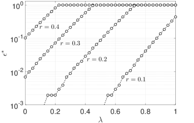
Figure 1: $\epsilon^{\star}$ versus $\lambda$ for $r=0.1$, $0.2$, $0.3$, and $0.4$

V-B Network Design

Then we solve the network design for stabilization, i.e., Problem II.2, using Theorem IV.1. Here we assume that $r_{ij}$ depends only on $i$, i.e., $r_{ij}=r_{i}$ for all $j\in[N]$. Under this assumption, we can choose the posynomial functions $\eta_{ij}$, $\Phi_{ij}$, and $\Psi_{ij}$ satisfying (6) as $\eta_{ij}=a_{ij}(\bar{\beta}-\underaccent{\bar}{\beta})$ and $\Phi_{ij}=\Psi_{ij}=a_{ij}r_{i}(\bar{\beta}-\underaccent{\bar}{\beta})^{2}$ because we have

$$\lVert A_{ij}-E[A_{ij}]\rVert=a_{ij}\max(r_{i},1-r_{i})(\bar{\beta}-\underaccent{\bar}{\beta})$$

and $W(A_{ij})=W(A_{ij}^{\top})=a_{ij}r_{i}(1-r_{i})(\bar{\beta}-\underaccent{\bar}{\beta})^{2}$.

We put the constraint $\epsilon\leq 0.2$, i.e., we require that the resulting optimal parameter $r^{\star}$ guarantees stability of with probability at least $0.8$. This constraint is equivalent to the monomial constraint:

$$f_{1}=\frac{\log(N/(0.2))}{\rho}\leq 1.$$

We use the cost function $R=\sum_{i=1}^{N}({1}/{r_{i}})$. With these parameters, we solve the geometric program (7) and find the optimal non-prevention probabilities $r_{1}^{\star}$, $\dotsc$, $r_{N}^{\star}$. Fig. 2 shows the value of the obtained $r^{\star}$ versus the in-degree of the nodes. From the figure we can see that, the edges pointing toward a node with the larger in-degree should receive protection resource with the larger probability.

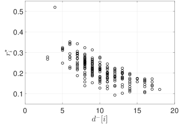
Figure 2: In-degrees and optimal probabilities

VI Conclusion

We have studied the stability of the networks of positive linear systems subject to time-invariant and random uncertainty. We have first presented a collection of linear matrix inequalities to study the stability of the whole network around the origin with a given probability and a decay rate. Based on this result, we have then proposed a convex optimization framework to optimally design the parameters of the probability distribution that describes the uncertainty of the system. We have illustrated our results using a networked susceptible-infected-susceptible viral spreading model.

References

- [1] B. R. Barmish, “Generalization of Kharitonov’s four-polynomial concept for robust stability problems with linearly dependent coefficient perturbations,” IEEE Transactions on Automatic Control, vol. 34, pp. 157–165, 1989.
- [2] J. Bernussou, P. Peres, and J. Geromel, “A linear programming oriented procedure for quadratic stabilization of uncertain systems,” Systems & Control Letters, vol. 13, pp. 65–72, 1989.
- [3] P. Gahinet, P. Apkarian, and M. Chilali, “Affine parameter-dependent Lyapunov functions and real parametric uncertainty,” IEEE Transactions on Automatic Control, vol. 41, pp. 436–442, 1996.
- [4] D. C. W. Ramos and P. L. D. Peres, “An LMI condition for the robust stability of uncertain continuous-time linear systems,” IEEE Transactions on Automatic Control, vol. 47, pp. 675–678, 2002.
- [5] M. de Oliveira, J. Bernussou, and J. Geromel, “A new discrete-time robust stability condition,” Systems & Control Letters, vol. 37, pp. 261–265, 1999.
- [6] R. C. Oliveira and P. L. Peres, “LMI conditions for robust stability analysis based on polynomially parameter-dependent Lyapunov functions,” Systems & Control Letters, vol. 55, pp. 52–61, 2006.
- [7] J. Lavaei and A. G. Aghdam, “Robust stability of LTI systems over semialgebraic sets using sum-of-squares matrix polynomials,” IEEE Transactions on Automatic Control, vol. 53, pp. 417–423, 2008.
- [8] C. Briat, “Robust stability and stabilization of uncertain linear positive systems via integral linear constraints: -gain and -gain characterization,” International Journal of Robust and Nonlinear Control, 2012.
- [9] M. Colombino, A. B. Hempel, and R. S. Smith, “Robust stability of a class of interconnected monlinear positive systems,” in 2015 American Control Conference, 2015, pp. 5312–5317.
- [10] R. Shorten, O. Mason, and C. King, “An alternative proof of the Barker, Berman, Plemmons (BBP) result on diagonal stability and extensions,” Linear Algebra and Its Applications, vol. 430, pp. 34–40, 2009.
- [11] B. Spencer, M. Sain, C.-H. Won, D. Kaspari, and P. Sain, “Reliability-based measures of structural control robustness,” Structural Safety, vol. 15, pp. 111–129, 1994.
- [12] Y.-G. Zhao and T. Ono, “A general procedure for first/second-order reliabilitymethod (FORM/SORM),” Structural Safety, vol. 21, pp. 95–112, 1999.
- [13] S. Boyd, S.-J. Kim, L. Vandenberghe, and A. Hassibi, “A tutorial on geometric programming,” Optimization and Engineering, vol. 8, pp. 67–127, 2007.
- [14] P. Van Mieghem, J. Omic, and R. Kooij, “Virus spread in networks,” IEEE/ACM Transactions on Networking, vol. 17, pp. 1–14, 2009.
- [15] R. Pastor-Satorras, C. Castellano, P. Van Mieghem, and A. Vespignani, “Epidemic processes in complex networks,” Reviews of Modern Physics, vol. 87, pp. 925–979, 2015.
- [16] M. Garetto, W. Gong, and D. Towsley, “Modeling malware spreading dynamics,” in IEEE INFOCOM 2003. Twenty-second Annual Joint Conference of the IEEE Computer and Communications Societies, vol. 3, 2003, pp. 1869–1879.
- [17] K. Lerman and R. Ghosh, “Information contagion: An empirical study of the spread of news on Digg and Twitter social networks,” in Proceedings of the Fourth International AAAI Conference on Weblogs and Social Media, 2010, pp. 90–97.
- [18] F. Chung and M. Radcliffe, “On the spectra of general random graphs,” The Electronic Journal of Combinatorics, vol. 18, #P215, 2011.
- [19] L. Farina and S. Rinaldi, Positive Linear Systems: Theory and Applications. Wiley-Interscience, 2000.
- [20] J. Brewer, “Kronecker products and matrix calculus in system theory,” IEEE Transactions on Circuits and Systems, vol. 25, pp. 772–781, 1978.
- [21] C. Metcalf, V. Andreasen, O. Bjørnstad, K. Eames, W. Edmunds, S. Funk, T. Hollingsworth, J. Lessler, C. Viboud, and B. Grenfell, “Seven challenges in modelling vaccine preventable diseases,” Epidemics, pp. 3–7, 2014.
- [22] F. M. G. Magpantay, M. A. Riolo, M. D. de Cellès, A. A. King, and P. Rohani, “Epidemiological consequences of imperfect vaccines for immunizing infections,” SIAM Journal on Applied Mathematics, vol. 74, pp. 1810–1830, 2014.
- [23] V. M. Preciado, M. Zargham, C. Enyioha, A. Jadbabaie, and G. J. Pappas, “Optimal resource allocation for network protection against spreading processes,” IEEE Transactions on Control of Network Systems, vol. 1, pp. 99–108, 2014.